Using Generalized Generation Distribution Factors in a MILP Model to Solve the Transmission-Constrained Unit Commitment Problem

Abstract

This study proposes a mixed-integer linear programming (MILP) model to figure out the transmission-constrained direct current (DC)-based unit commitment (UC) problem using the generalized generation distribution factors (GGDF) for modeling the transmission network constraints. The UC problem has been reformulated using these linear distribution factors without sacrificing optimality. Several test power systems (PJM 5-bus, IEEE-24, and 118-bus) have been used to validate the introduced formulation. Results demonstrate that the proposed approach is more compact and less computationally burdensome than the classical DC-based formulation, which is commonly employed in the technical literature to carry out the transmission network constraints. Therefore, there is a potential applicability of the accomplished methodology to carry out the UC problem applied to medium and large-scale electrical power systems.

1. Introduction

The unit commitment (UC) optimization problem is the conventional formulation used by regulated companies and power pools to schedule the power generation units for supplying the load demand over a multi-hour to multi-day timeframe [1]. The UC problem consists of deciding which thermoelectric power units need to operate at each time period (1 h) in order to minimize the generation costs (fuel cost, startup, and shutdown costs), and to satisfy the operational technical constraints for the entire power system (spinning reserve and load), as well as for each power generation unit (minimum up/down times, minimum and maximum power, and load ramps) [2].

1.1. Literature Review

It is critical that transmission power flow constraints will be incorporated in the UC formulation, because most power grids are operating close to their security electrical margins [3]. Different linear transmission network formulations have been apply to model the transmission capacity limits in the UC optimization problem. However, most researchers use the classical DC-based power flow formulation [4,5,6,7,8,9,10,11,12,13], where the active power unit generation and the voltage phase angles are the decision variables used to carry out the operational problem. This problem consists of two analyses: (1) the nodal power balance equality constraints; and (2) the maximum transmission power flow inequality constraints. Based on the classical DC-based formulation and incorporating the transmission power flow constraints in the optimization problem, it is significantly increased the problem size becoming computationally more complex when it is applied to large-scale electrical power systems.

Determining the transmission power flow relationships, constraints and variables that have no influence in the mathematical formulation could be eliminated from the optimization problem [6]. Alternatively, linear sensitivity factors (LSF) have also been used in the technical literature [14,15,16,17,18,19,20,21] to determine the active power network constraints in the UC problem. The LSF formulation has the advantage of requiring fewer decision variables, as well as equality constraints, by excluding the phase voltage angles without sacrificing optimality. Nevertheless, the power flow sensitivity matrix is not sparse, and it could be precomputed offline and updated when the network topology changes due to an outage, maintenance, or a switching event [17].

The LSF are also known as partial transmission distribution factors (PTDF), and these linear factors are used to carry out the transmission-constrained UC problem by several researchers in the technical literature. In addition, this approach does not sacrifice the optimality in the mathematical formulation; i.e., the equivalence for both models has been demonstrated in several studies [12,20].

An algorithm for solving the UC problem by means of the Lagrangian relaxation approach is reported in [13], where the transmission power flow constraints are formulated as linear inequality constraints based on the LSF and the net power injected in each electrical bus. A similar approach is implemented in a three-phase algorithmic scheme to determine the UC problem reported in [16]. Benders decomposition is proposed in [15] for solving the UC problem. The transmission-constrained UC problem is decomposed into two problems: a master problem and a subproblem. The master problem solves the UC without transmission network limits using the augmented Lagrangian relaxation, and the subproblem must accomplish the transmission inequality constraints. In this study, the transmission power flow constraints are also formulated as linear constraints using the PTDF. On the other hand, a method for treating transmission network bottlenecks in a stochastic market model, where generators and loads are allocated into regional sub-systems or price areas, is reported in [18]. The market model is designed for long-term and medium-term scheduling of hydrothermal power system operation. When any of the interconnections are overloaded, power flow constraints are added to the area optimization problem using the PTDF. An effective approach for obtaining robust solutions to the security-constrained (SC) UC problem with load and wind uncertainty correlation is proposed in [19]. The SCUC model is solved by Benders decomposition. Transmission network constraints are modeled using the PTDF. A power-based network constrained UC model to deal with wind generation uncertainty is reported in [20]. The model schedules power-trajectories instead of the traditional energy-blocks, and it takes into account the inherent startup and shutdown power trajectories of thermal units. The PTDF are used to model the active power flow constraints. Additionally, an N–1 security-constrained UC approach is reported in [21]. The transmission constraints are formulated as linear constraints based on the classical DC power flow approach. The transmission-constrained UC problem is determined using the injection shift factors for modeling the pre-contingency constraints and the line outage distribution factors (LODF) for modeling the post-contingency power flow constraints (N–1 criterion).

1.2. Contributions

This study proposes to apply the GGDF, which are another LSF used to formulate the network transmission inequality constraints in the unit commitment problem. The GGDF relates the active power flow in the transmission lines or transformers with the generation power unit for a given electrical system [22]. In comparison with the PTDF-based formulation, the main advantage of the GGDF-based formulation is that the definition of the active power flow inequality constraints is enhanced. Notice that these linear distribution factors represent the portion of generation supplied by each power unit that flows on a specific transmission line. Another advantage is that, unlike PTDF, which uses a slack bus to calculate these values, the obtained GGDF is the same matrix using any slack bus to compute these factors. It is worth highlighting that, in the GGDF-based formulation: (1) the nodal power balance equality constraints are transformed using only one equality constraint, which is also used in the economic dispatch problem to supply the load of the customers; and (2) the transmission power flow inequality constraints are carried out using the GGDF and the active power generation of each unit. It should be also pointed out that the active power generation is the only decision variable in the operational optimization problem.

In the technical literature review, there is no evidence about the performance of the GGDF-based formulation applied to the transmission-constrained UC problem. In this study, the accuracy and performance of UC GGDF-based formulation are gauged and compared to both the classical DC- and PTDF-based formulations. It has accomplished several analyses by means of the proposed methodology and a commercial solver in order to evaluate the performance of the formulation applied to PJM 5-bus, IEEE-24, and 118-bus power systems. The results demonstrate that a superior performance is achieved for modeling medium-scale power systems and, mainly, it has improved the mathematical complexity of the optimization problem given in [12], as well as bringing great practical advantages for modeling the stochastic scheduling problems without sacrificing the UC optimality.

This paper is structured as follows: Section 2 presents the UC optimization problem, and Section 3 describes the simulation results. Finally, Section 4 concludes and suggests directions for future work.

2. Transmission-Constrained Unit Commitment (TCUC) Model

2.1. Linearized Generator Cost Modeling

The total generation cost is typically expressed as a quadratic cost curves (QCCs). To facilitate the UC optimization process with efficient mixed-integer linear programing (MILP) solvers, QCCs are piecewise linearized.

Unit i’s production cost function is given by the following equation:

$$C\left(p_i\right)={\alpha }_i+{\beta }_i{p}_i+{\gamma }_i{p}_i^2$$

(1)

where $C\left(p_i\right)$ is the total generation cost, $p_i$ is the output power of the generator $i,$ and ${\alpha }_i,{\beta }_i,$ and ${\gamma }_i$ are the production cost factors. The generator total cost curve can be represented by a series of linear sections [23]. The linearized generator cost model could be mathematically formulated as follows:

$$p_i={\displaystyle \sum _{l=1}^{Lg}\Delta p_{i,l}}$$

(2)

$$0\le \Delta p_{i,l}\le \frac{P_i^{Max}}{Lg}$$

(3)

$$C\left(p_i\right)={\alpha }_i+{\displaystyle \sum _{l=1}^{Lg}{k}_{i,l}\Delta p_{i,l}}$$

(4)

$$k_{i,l}={\beta }_i+(2l-1){\gamma }_i\left(\frac{P_i^{Max}}{Lg}\right)$$

(5)

where $\Delta p_{i,l}$ represent segments of the i-th output power unit, $P_i^{Max}$ is the maximum power generation of unit $i,$ $k_{i,l}$ is a linear section in the total cost curve, and $Lg$ is the number of segments.

2.2. Transmission Network Modeling

Most popular UC implementations have adopted the classical DC-based formulation to carry out: (1) the nodal power balance constraints; and (2) the transmission network constraints.

(1)

In the classical DC-based formulation, the power balance equality constraints are formulated using the following matrix equation:

$$B\theta =P-Pd$$

(6)

where $B$ is the bus admittance matrix, $\theta$ is the vector of node phase angles, $P$ is a power generation vector, and $Pd$ is a power demand vector.

However, when the voltage phase angles are replaced in Equation (6) using the inverse of the admittance matrix $B$, only one equation is obtained to supply the load of the customers for both the PTDF- and GGDF-based formulations.

(2)

Using the classical DC approach, the power flow, $P_{mq}$, through the transmission line between bus m and q, is defined using Equation (7):

$$P_{mq}=\frac{{\theta }_m-{\theta }_q}{X_{mq}}=B_{mq}\left({\theta }_m-{\theta }_q\right)$$

(7)

where ${\theta }_m$ is the complex voltage angle at bus m, $B_{mq}$ is the line susceptance between buses m–q, and $X_{mq}$ is the line reactance between buses m–q.

Based on the technical literature review, the transmission power flows can also be expressed using the PTDF matrix as [12,24,25]:

$$P_{mq}=PTDF\left(A_g^{t}P-Pd\right)$$

(8)

where $A_g$ is the generator-bus incidence matrix.

The PTDF matrix is a function of the transmission lines impedances. In addition, the PTDF matrix depends on a slack bus, which means that for any choice of slack bus, there will be a PTDF matrix that completely describes how the injections at each bus in the network affect the power flows throughout the transmission system. Note that every power injection is compensated by the slack bus.

It is worth mentioning that the PTDF factors must be precomputed and stored prior to the mathematical formulation and simulation.

On the other hand, the power flow through the transmission line between bus m and n, could be expressed using the GGDF [26]:

$$P_{mq}=GGD{F}_{mq,i}{p}_i$$

(9)

where the GGDF represents the portion of generation supplied by each generator that flows on a specific transmission line.

For any mathematical formulation, the maximum transmission power flows must be constrained considering the transmission thermal limits:

$$-P_{mq}^{Max}\le P_{mq}\le P_{mq}^{Max}\hspace{1em}\forall m,q\in N$$

(10)

where $N$ is the total number of buses, and $P_{mq}^{Max}$ is the maximum power flow through the transmission line m–q.

Using the PTDF matrix, the transmission limit constraint is expressed as follows:

$$-P_{mq}^{Max}\le PTD{F}_{mq}\left(A_g^{t}P-Pd\right)\le P_{mq}^{Max}\hspace{1em}\forall m,q\in N$$

(11)

Since the load of the customers is constant values for each time period; i.e., they are not affected by the UC problem so that they can be accordingly moved from Equation (11) to the left-hand (lhs) and right-hand (rhs) limits.

Using the GGDF matrix, the transmission limit constraints are expressed using the following equation:

$$-P_{mq}^{Max}\le GGD{F}_{mq,i}{p}_i\le P_{mq}^{Max}\hspace{1em}\forall m,q\in N$$

(12)

Notice that previous task is avoided using the GGDF formulation, because the transmission power flows are only a function of GGDF and decision variables (active power generation of each unit).

See the Appendix A for a detailed derivation of the GGDF matrix.

In order to compare the three formulations, we show how to model, for a given period t, the nodal power balance equality constraints and the transmission power flow inequality constraints. Every formulation has been applied to the PJM 5-bus system, which is included in Matpower [27]. For the transmission network modeling, bus 1 has been used as the reference (slack) bus and a base power value of 100 MVA.

(1)

Classical DC-based formulation using p.u. values:

$$B_{bus}\left[\begin{array}{c}{\theta }_1\\ {\theta }_2\\ {\theta }_3\\ \begin{array}{l}{\theta }_4\\ {\theta }_5\end{array}\end{array}\right]=\left[\begin{array}{c}{P}_1-P{d}_1\\ P_2-P{d}_2\\ P_3-P{d}_3\\ \begin{array}{l}{P}_4-P{d}_4\\ P_5-P{d}_5\end{array}\end{array}\right]$$

$$\begin{array}{c}-4\le \frac{{\theta }_1-{\theta }_2}{0.0281}\le 4\\ -10\le \frac{{\theta }_1-{\theta }_4}{0.0304}\le 10\\ -10\le \frac{{\theta }_1-{\theta }_5}{0.0064}\le 10\\ -10\le \frac{{\theta }_2-{\theta }_3}{0.0108}\le 10\\ -10\le \frac{{\theta }_3-{\theta }_4}{0.0297}\le 10\\ -2.4\le \frac{{\theta }_4-{\theta }_5}{0.0297}\le 2.4\end{array}$$

(2)

The PTDF-based formulation using MW values:

$$P_1+P_2+P_3+P_4+P_5=P_D$$

$$-\left[\begin{array}{c}400\\ 1000\\ 1000\\ 1000\\ 1000\\ 240\end{array}\right]\le PTDF\left[\begin{array}{c}{P}_1-P{d}_1\\ P_2-P{d}_2\\ P_3-P{d}_3\\ \begin{array}{l}{P}_4-P{d}_4\\ P_5-P{d}_5\end{array}\end{array}\right]\le \left[\begin{array}{c}400\\ 1000\\ 1000\\ 1000\\ 1000\\ 240\end{array}\right]$$

(3)

The GGDF-based formulation using MW values:

$$P_1+P_2+P_3+P_4+P_5=P_D$$

$$-\left[\begin{array}{c}400\\ 1000\\ 1000\\ 1000\\ 1000\\ 240\end{array}\right]\le GGDF\left[\begin{array}{c}{P}_1\\ P_2\\ P_3\\ \begin{array}{l}{P}_4\\ P_5\end{array}\end{array}\right]\le \left[\begin{array}{c}400\\ 1000\\ 1000\\ 1000\\ 1000\\ 240\end{array}\right]$$

where:

$$B_{bus}=\left[\begin{array}{ccccc}224.7319& -35.5872& 0& -32.8947& -156.2500\\ -35.5872& 128.1798& -92.5926& 0& 0\\ 0& -92.5926& 126.2626& -33.6700& 0\\ \begin{array}{l}-32.8947\\ -156.2500\end{array}& \begin{array}{l}0\\ 0\end{array}& \begin{array}{l}-33.6700\\ 0\end{array}& \begin{array}{l}100.2348\\ -33.6700\end{array}& \begin{array}{l}-33.6700\\ 189.9200\end{array}\end{array}\right]$$

$$PTDF=\left[\begin{array}{ccccc}0& -0.6698& -0.5429& -0.1939& -0.0344\\ 0& -0.1792& -0.2481& -0.4376& -0.0776\\ 0& -0.1509& -0.2090& -0.3685& -0.8880\\ 0& 0.3302& -0.5429& -0.1939& -0.0344\\ 0& 0.3302& 0.4571& -0.1939& -0.0344\\ 0& 0.1509& 0.2090& 0.3685& -0.1120\end{array}\right]$$

$$GGDF=\left[\begin{array}{ccccc}0.4414& -0.2284& -0.1015& 0.2475& 0.4070\\ 0.3032& 0.1240& 0.0551& -0.1343& 0.2257\\ 0.2554& 0.1044& 0.0464& -0.1131& -0.6327\\ 0.1414& 0.4716& -0.4015& -0.0525& 0.1070\\ -0.1586& 0.1716& 0.2985& -0.3525& -0.1930\\ -0.2554& -0.1044& -0.0464& 0.1131& -0.3673\end{array}\right]$$

It should be pointed out that the equality and inequality constraints are equivalent for each formulation without sacrificing the UC optimality.

2.3. TCUC Mathematical Formulation

This paper uses the MILP formulation introduced in [28] as the reference formulation for the UC problem. The proposed TCUC model using the GGDF is mathematically formulated as follows:

$$Min{\displaystyle \sum _{t=1}^T{\displaystyle \sum _{i=1}^{Ng}\left[{\alpha }_i{I}_{i,t}+{\displaystyle \sum _{j=1}^{Lg}{k}_{ij}\Delta p_{ij,t}}+c_{i,t}^U+c_{i,t}^D\right]}}+{\displaystyle \sum _{t=1}^T{\displaystyle \sum _{j=1}^N{c}_{j,t}^{ENS}}}$$

(13)

$$\mathrm{subject} \mathrm{to}\text{:} {\displaystyle \sum _{i=1}^{Ng}{p}_{i,t}}+{\displaystyle \sum _{j=1}^{N}EN{S}_{i,t}}={\displaystyle \sum _{i=1}^{N}P{d}_{i,t}}\hspace{1em}\forall t\in T$$

(14)

$${\displaystyle \sum _{i=1}^{Ng}{p}_{i,t}\ge }{\displaystyle \sum _{i=1}^{N}P{d}_{i t}}+R_t\hspace{1em}\forall t\in T$$

(15)

$$p_{i,t}={\displaystyle \sum _{ij=1}^{Lg}\Delta p_{ij,t}}\hspace{1em}\forall i\in Ng$$

(16)

$$0\le \Delta p_{ij}\le \frac{P_i^{Max}}{Lg}\hspace{1em}\forall j\in Lg$$

(17)

$${\overline{p}}_{i,t}\le P_i^{Max}\left[I_{i,t}-z_{i,(t+1)}\right]+z_{i,(t+1)}S{D}_i\hspace{1em}\forall t\in T$$

(18)

$${\overline{p}}_{i,t}\le p_{i,\left(t-1\right)}+R{U}_i{I}_{i,(t-1)}+S{U}_i{y}_{i,t}\hspace{1em}\forall t\in T$$

(19)

$${\overline{p}}_{i,t}\ge 0\hspace{1em}\forall t\in T$$

(20)

$$p_{i,t}\le {\overline{p}}_{i,t}\hspace{1em}\forall t\in T$$

(21)

$$P_i^{Min}{I}_{i,t}\le p_{i,t}\hspace{1em}\forall t\in T$$

(22)

$$p_{i,\left(t-1\right)}-p_{i,t}\le R{D}_i{I}_{i,t}+S{D}_i{z}_{i,t}\hspace{1em}\forall t\in T$$

(23)

$${\displaystyle \sum _{t=1}^{F_i}{I}_{i,t}}=0 \mathrm{where} F_i=Min\left\{\left[T,\left(D{T}_i-s_{i,0}\right)\right]\left[1-I_{i,0}\right]\right\}$$

(24)

$${\displaystyle \sum _{n=t}^{t+D{T}_i-1}\left[1-I_{i,t}\right]}\ge D{T}_i{z}_{i,t}\hspace{1em}\forall t=F_{i+1}\dots T-D{T}_{t+1}$$

(25)

$${\displaystyle \sum _{n=t}^T\left[1-I_{i,n}-z_{i,t}\right]\ge }0\hspace{1em}\forall t=T-D{T}_{i+2}\dots T$$

(26)

$${\displaystyle \sum _{t=1}^{L_i}\left[1-I_{i,t}\right]}=0 \mathrm{where} L_i=Min\left[T,\left(U{T}_i-U_{i,0}\right)I_{i,0}\right]$$

(27)

$${\displaystyle \sum _{n=t}^{t+U{T}_i-1}{I}_{i,n}}\ge U{T}_i{y}_{i,t}\hspace{1em}\forall t=L_{i+1}\dots T-U{T}_{t+1}$$

(28)

$${\displaystyle \sum _{n=t}^T\left[I_{i,n}-y_{i,n}\right]\ge }0\hspace{1em}\forall t=T-U{T}_{i+2}\dots T$$

(29)

$$-P_{mq,t}^{Max}\le GGDF{p}_{i,t}\le P_{mq,t}^{Max}\hspace{1em}\forall t\in T$$

(30)

$$y_{i,t}-z_{i,t}=I_{i,t}-I_{i,t-1}\hspace{1em}\forall t\in T$$

(31)

$$y_{i,t}+z_{i,t}\le 1\hspace{1em}\forall t\in T$$

(32)

where $Ng$ is the total number of generators, $T$ is the total number of periods; $c_{i,t}^U,c_{i,t}^D$ are the startup and shutdown costs of unit i at period t ($), respectively; $c_{j,t}^{ENS}$ is the non-served energy cost of bus j at period t ($/MWh); $P{d}_{i t}$ is the load demand of node i at period t (MW); $R_t$ is the system spinning reserve at period t (MW); $P_i^{Min}$ is the minimum output power of unit $i$ (MW); $S{U}_i$ and $S{D}_i$ are the startup and shutdown ramp limits of unit i (MW/h), respectively; $R{U}_i$ and $R{D}_i$ are the ramp-up and ramp-down rate limits of unit i (MW/h), respectively; $U{T}_i$ and $D{T}_i$ are the minimum up and down time of unit i (h), respectively; $I_{i,t}$ is a binary variable equal to 1 for period t whether unit i is on and 0 otherwise (off); $y_{i,t}$ is a binary variable equal to 1 whether unit i is started up at the beginning of period t and 0 otherwise; and $z_{i,t}$ is a binary variable equal to 1 whether unit i is shutdown at the beginning of period t and 0 otherwise.

The objective function in Equation (13) minimizes the variable production costs, the startup and shutdown costs and the non-served energy cost. The UC problem is subject to the following equality and inequality constraints: load balance equality constraint (Equation (14)), system spinning reserve (Equation (15)), linearized production cost (Equations (16) and (17)), limits on power output (Equations (21) and (22)), generators’ ramp rate (Equations (18)–(20) and (23)), generators’ minimum downtime (Equations (24)–(26)), generators’ minimum uptime (Equations (27)–(29)), transmission network (Equation (30)), and commitment, as well as startup and shutdown logic, of generating units (Equations (31)–(32)).

3. Results

In this section, the introduced mathematical formulation is applied to three electrical test systems: the PJM 5-bus system, the IEEE 24-bus reliability test system, as well as the IEEE 118-bus system. The proposed transmission-constrained UC approach is compared in terms of unit commitment costs and computational aspects using results obtained by other methodologies [12].

All simulations are performed on a personal computer (PC) running Windows^® 10 with an Intel^® Core i7, 2.7-GHz, 12 GB RAM, and 64-bit, using CPLEX^® (12.7.1) under MATLAB^® Code (Version 2014b, ITM, Mexico). Computing the simulation time is based on a set of 100 simulations.

3.1. PJM 5-Bus System

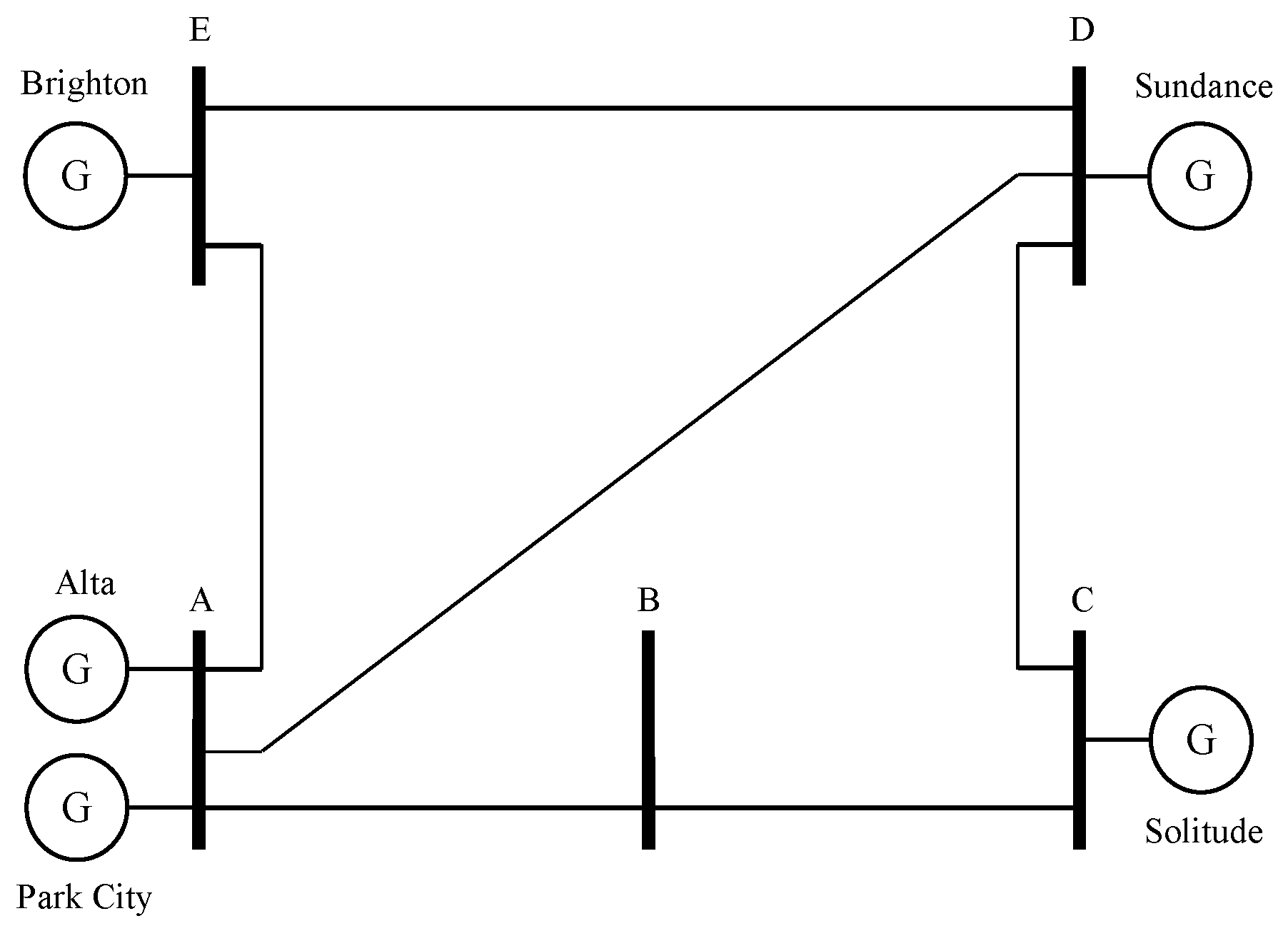
The PJM 5-bus system has five buses, six transmission lines, and five generators. Operational costs and system data are taken from [29]. Figure 1 depicts the one-line diagram for this system. In this test system, the spinning capacity requirements are set to $R_t=0.03{\displaystyle \sum _{i=1}^{N}P{d}_{i t}}$ for all time periods (t).

Table 1. Minimum up (UT) and down (DT) times.

Unit #	$\mathit{U}{\mathit{T}}_{\mathit{i}} \left(\mathbf{hours}\right)$	$\mathit{D}{\mathit{T}}_{\mathit{i}} \left(\mathbf{hours}\right)$	Initial Condition (hours)
Alta	5	3	0
Park City	5	3	0
Solitude	4	2	8
Sundace	3	2	8
Brighton	5	4	0

lists the minimum up and down times and initial conditions for each power unit.

The hourly load percentage levels are taken from [30] (Table 4—RTS 96 system). The system’s peak demand occurs at hour 21, and the minimum demand occurs at hour 4.

To fully illustrate the TCUC problem applied to this power system, the following mathematical equations have been presented in order to explain the optimization problem given in Equations (13)–(32):

$$Min{\displaystyle \sum _{t=1}^{24}}\left[\begin{array}{l}{\alpha }_{\mathrm{Brighton}}{I}_{i,t}+{\displaystyle \sum _{j=1}^{Lg}{k}_{\mathrm{Brighton} j}\Delta p_{\mathrm{Brighton} j,t}}+c_{\mathrm{Brighton},t}^U+c_{\mathrm{Brighton},t}^D\\ {\alpha }_{\mathrm{Sundance}}{I}_{\mathrm{Sundance},t}+{\displaystyle \sum _{j=1}^{Lg}{k}_{\mathrm{Sundance} j}\Delta p_{\mathrm{Sundance} j,t}}+c_{\mathrm{Sundance},t}^U+c_{\mathrm{Sundance},t}^D\\ {\alpha }_{\mathrm{Alt}a}{I}_{\mathrm{Alt}a,t}+{\displaystyle \sum _{j=1}^{Lg}{k}_{\mathrm{Alta} j}\Delta p_{\mathrm{Alta} j,t}}+c_{\mathrm{Alta},t}^U+c_{\mathrm{Alta},t}^D\\ \begin{array}{l}{\alpha }_{\mathrm{Park} \mathrm{City}}{I}_{\mathrm{Park} \mathrm{City},t}+{\displaystyle \sum _{j=1}^{Lg}{k}_{\mathrm{Park} \mathrm{City} j}\Delta p_{\mathrm{Park} \mathrm{City} j,t}}+c_{\mathrm{Park} \mathrm{City},t}^U+c_{\mathrm{Park} \mathrm{City},t}^D\\ {\alpha }_{\mathrm{Solitude}}{I}_{\mathrm{Solitude},t}+{\displaystyle \sum _{j=1}^{Lg}{k}_{\mathrm{Solitude} j}\Delta p_{\mathrm{Solitude} j,t}}+c_{\mathrm{Solitude},t}^U+c_{\mathrm{Solitude},t}^D\end{array}\end{array}\right]$$

$$p_{\mathrm{Brighton},t}+p_{\mathrm{Sundance},t}+p_{\mathrm{Alta},t}+p_{\mathrm{Park} \mathrm{City},t}+p_{\mathrm{Solitude},t}={\displaystyle \sum _{i=1}^{N}P{d}_{i,t}}\hspace{1em}\forall t=1,\dots ,24$$

$$p_{\mathrm{Brighton},t}+p_{\mathrm{Sundance},t}+p_{\mathrm{Alta},t}+p_{\mathrm{Park} \mathrm{City},t}+p_{\mathrm{Solitude},t}\ge {\displaystyle \sum _{i=1}^{N}P{d}_{i t}}+R_t\hspace{1em}\forall t=1,\dots ,24$$

$$p_{\mathrm{Brighton},t}={\displaystyle \sum _{j=1}^{Lg}\Delta p_{\mathrm{Brighton} j,t}}\hspace{1em}\forall t=1,\dots ,24$$

$$p_{\mathrm{Sundance},t}={\displaystyle \sum _{j=1}^{Lg}\Delta p_{\mathrm{Sundance} j,t}}\hspace{1em}\forall t=1,\dots ,24$$

$$p_{\mathrm{Alta},t}={\displaystyle \sum _{j=1}^{Lg}\Delta p_{\mathrm{Alta} j,t}}\hspace{1em}\forall t=1,\dots ,24$$

$$p_{\mathrm{Park} \mathrm{City},t}={\displaystyle \sum _{j=1}^{Lg}\Delta p_{\mathrm{Park} \mathrm{City} j,t}}\hspace{1em}\forall t=1,\dots ,24$$

$$p_{\mathrm{Solitude},t}={\displaystyle \sum _{j=1}^{Lg}\Delta p_{\mathrm{Solitude} j,t}}\hspace{1em}\forall t=1,\dots ,24$$

$$0\le \Delta p_{\mathrm{Brighton} j,t}\le \frac{P_{\mathrm{Brighton}}^{Max}}{Lg}\hspace{1em}\forall j=1,\dots ,Lg$$

$$0\le \Delta p_{\mathrm{Sundance} j,t}\le \frac{P_{\mathrm{Sundance}}^{Max}}{Lg}\hspace{1em}\forall j=1,\dots ,Lg$$

$$0\le \Delta p_{\mathrm{Alta} j,t}\le \frac{P_{\mathrm{Alta}}^{Max}}{Lg}\hspace{1em}\forall j=1,\dots ,Lg$$

$$0\le \Delta p_{\mathrm{Park} \mathrm{City} j,t}\le \frac{P_{\mathrm{Park} \mathrm{City}}^{Max}}{Lg}\hspace{1em}\forall j=1,\dots ,Lg$$

$$0\le \Delta p_{\mathrm{Solitude} j,t}\le \frac{P_{\mathrm{Solitude}}^{Max}}{Lg}\hspace{1em}\forall j=1,\dots ,Lg$$

$${\overline{p}}_{\mathrm{Brighton},t}\le P_{\mathrm{Brighton}}^{Max}\left[I_{\mathrm{Brighton},t}-z_{\mathrm{Brighton},(t+1)}\right]+z_{\mathrm{Brighton},(t+1)}S{D}_{\mathrm{Brighton}}\hspace{1em}\forall t=1,\dots ,24$$

$${\overline{p}}_{\mathrm{Sundance},t}\le P_{\mathrm{Sundance}}^{Max}\left[I_{\mathrm{Sundance},t}-z_{\mathrm{Sundance},(t+1)}\right]+z_{\mathrm{Sundance},(t+1)}S{D}_{\mathrm{Sundance}}\hspace{1em}\forall t=1,\dots ,24$$

$${\overline{p}}_{\mathrm{Alta},t}\le P_{\mathrm{Alta}}^{Max}\left[I_{\mathrm{Alta},t}-z_{\mathrm{Alta},(t+1)}\right]+z_{\mathrm{Alta},(t+1)}S{D}_{\mathrm{Alta}}\hspace{1em}\forall t=1,\dots ,24$$

$${\overline{p}}_{\mathrm{Park} \mathrm{City},t}\le P_{\mathrm{Park} \mathrm{City}}^{Max}\left[I_{\mathrm{Park} \mathrm{City},t}-z_{\mathrm{Park} \mathrm{City},(t+1)}\right]+z_{\mathrm{Park} \mathrm{City},(t+1)}S{D}_{\mathrm{Park} \mathrm{City}}\hspace{1em}\forall t=1,\dots ,24$$

$${\overline{p}}_{\mathrm{Solitude},t}\le P_{\mathrm{Solitude}}^{Max}\left[I_{\mathrm{Solitude},t}-z_{\mathrm{Solitude},(t+1)}\right]+z_{\mathrm{Solitude},(t+1)}S{D}_{\mathrm{Solitude}}\hspace{1em}\forall t=1,\dots ,24$$

$${\overline{p}}_{\mathrm{Brighton},t}\le p_{\mathrm{Brighton},\left(t-1\right)}+R{U}_{\mathrm{Brighton}}{I}_{\mathrm{Brighton},(t-1)}+S{U}_{\mathrm{Brighton}}{y}_{\mathrm{Brighton},t}\hspace{1em}\forall t=1,\dots ,24$$

$${\overline{p}}_{\mathrm{Sundance},t}\le p_{\mathrm{Sundance},\left(t-1\right)}+R{U}_{\mathrm{Sundance}}{I}_{\mathrm{Sundance},(t-1)}+S{U}_{\mathrm{Sundance}}{y}_{\mathrm{Sundance},t}\hspace{1em}\forall t=1,\dots ,24$$

$${\overline{p}}_{\mathrm{Alta},t}\le p_{\mathrm{Alta},\left(t-1\right)}+R{U}_{\mathrm{Alta}}{I}_{\mathrm{Alta},(t-1)}+S{U}_{\mathrm{Alta}}{y}_{\mathrm{Alta},t}\hspace{1em}\forall t=1,\dots ,24$$

$${\overline{p}}_{\mathrm{Park} \mathrm{City},t}\le p_{\mathrm{Park} \mathrm{City},\left(t-1\right)}+R{U}_{\mathrm{Park} \mathrm{City}}{I}_{\mathrm{Park} \mathrm{City},(t-1)}+S{U}_{\mathrm{Park} \mathrm{City}}{y}_{\mathrm{Park} \mathrm{City},t}\hspace{1em}\forall t=1,\dots ,24$$

$${\overline{p}}_{\mathrm{Solitude},t}\le p_{\mathrm{Solitude},\left(t-1\right)}+R{U}_{\mathrm{Solitude}}{I}_{\mathrm{Solitude},(t-1)}+S{U}_{\mathrm{Solitude}}{y}_{\mathrm{Solitude},t}\hspace{1em}\forall t=1,\dots ,24$$

$${\overline{p}}_{\mathrm{Brighton},t}\ge 0\hspace{1em}\forall t=1,\dots ,24$$

$${\overline{p}}_{\mathrm{Sundance},t}\ge 0\hspace{1em}\forall t=1,\dots ,24$$

$${\overline{p}}_{\mathrm{Alta},t}\ge 0\hspace{1em}\forall t=1,\dots ,24$$

$${\overline{p}}_{\mathrm{Park} \mathrm{City},t}\ge 0\hspace{1em}\forall t=1,\dots ,24$$

$${\overline{p}}_{\mathrm{Solitude},t}\ge 0\hspace{1em}\forall t=1,\dots ,24$$

$$p_{\mathrm{Brighton},t}\le {\overline{p}}_{\mathrm{Brighton},t}\hspace{1em}\forall t=1,\dots ,24$$

$$p_{\mathrm{Sundance},t}\le {\overline{p}}_{\mathrm{Sundance},t}\hspace{1em}\forall t=1,\dots ,24$$

$$p_{\mathrm{Alta},t}\le {\overline{p}}_{\mathrm{Alta},t}\hspace{1em}\forall t=1,\dots ,24$$

$$p_{\mathrm{Park} \mathrm{City},t}\le {\overline{p}}_{\mathrm{Park} \mathrm{City},t}\hspace{1em}\forall t=1,\dots ,24$$

$$p_{\mathrm{Solitude},t}\le {\overline{p}}_{\mathrm{Solitude},t}\hspace{1em}\forall t=1,\dots ,24$$

$$P_{\mathrm{Brighton}}^{Min}{I}_{\mathrm{Brighton},t}\le p_{\mathrm{Brighton},t}\hspace{1em}\forall t=1,\dots ,24$$

$$P_{\mathrm{Sundance}}^{Min}{I}_{\mathrm{Sundance},t}\le p_{\mathrm{Sundance},t}\hspace{1em}\forall t=1,\dots ,24$$

$$P_{\mathrm{Alta}}^{Min}{I}_{\mathrm{Alta},t}\le p_{\mathrm{Alta},t}\hspace{1em}\forall t=1,\dots ,24$$

$$P_{\mathrm{Park} \mathrm{City}}^{Min}{I}_{\mathrm{Park} \mathrm{City},t}\le p_{\mathrm{Park} \mathrm{City},t}\hspace{1em}\forall t=1,\dots ,24$$

$$P_{\mathrm{Solitude}}^{Min}{I}_{\mathrm{Solitude},t}\le p_{\mathrm{Solitude},t}\hspace{1em}\forall t=1,\dots ,24$$

$${\displaystyle \sum _{j=k}^{k+D{T}_{\mathrm{Brighton}}-1}\left[1-I_{\mathrm{Brighton},j}\right]}\ge D{T}_{\mathrm{Brighton}}{z}_{\mathrm{Brighton},k}\hspace{1em}\forall k=F_{i+1}\dots 24-D{T}_{j+1}$$

$${\displaystyle \sum _{j=k}^{k+D{T}_{\mathrm{Sundance}}-1}\left[1-I_{\mathrm{Sundance},j}\right]}\ge D{T}_{\mathrm{Sundance}}{z}_{\mathrm{Sundance},k}\hspace{1em}\forall k=F_{i+1}\dots 24-D{T}_{j+1}$$

$${\displaystyle \sum _{j=k}^{k+D{T}_{\mathrm{Alta}}-1}\left[1-I_{\mathrm{Alta},j}\right]}\ge D{T}_{\mathrm{Alta}}{z}_{\mathrm{Alta},k}\hspace{1em}\forall k=F_{i+1}\dots 24-D{T}_{j+1}$$

$${\displaystyle \sum _{j=k}^{k+D{T}_{\mathrm{Park} \mathrm{City}}-1}\left[1-I_{\mathrm{Park} \mathrm{City},j}\right]}\ge D{T}_{\mathrm{Park} \mathrm{City}}{z}_{\mathrm{Park} \mathrm{City},k}\hspace{1em}\forall k=F_{i+1}\dots 24-D{T}_{j+1}$$

$${\displaystyle \sum _{j=k}^{k+D{T}_{\mathrm{Solitude}}-1}\left[1-I_{\mathrm{Solitude},j}\right]}\ge D{T}_{\mathrm{Solitude}}{z}_{\mathrm{Solitude},k}\hspace{1em}\forall k=F_{i+1}\dots 24-D{T}_{j+1}$$

$${\displaystyle \sum _{j=k}^T\left[1-I_{\mathrm{Brighton},j}-z_{\mathrm{Brighton},k}\right]\ge }0\hspace{1em}\forall k=24-D{T}_{i+2}\dots 24$$

$${\displaystyle \sum _{j=k}^T\left[1-I_{\mathrm{Sundance},j}-z_{\mathrm{Sundance},k}\right]\ge }0\hspace{1em}\forall k=24-D{T}_{i+2}\dots 24$$

$${\displaystyle \sum _{j=k}^T\left[1-I_{\mathrm{Alta},j}-z_{\mathrm{Alta},k}\right]\ge }0\hspace{1em}\forall k=24-D{T}_{i+2}\dots 24$$

$${\displaystyle \sum _{j=k}^T\left[1-I_{\mathrm{Park} \mathrm{City},j}-z_{\mathrm{Park} \mathrm{City},k}\right]\ge }0\hspace{1em}\forall k=24-D{T}_{i+2}\dots 24$$

$${\displaystyle \sum _{j=k}^T\left[1-I_{\mathrm{Solitude},j}-z_{\mathrm{Solitude},k}\right]\ge }0\hspace{1em}\forall k=24-D{T}_{i+2}\dots 24$$

$$\begin{array}{c}{\displaystyle \sum _{j=k}^{k+U{T}_{\mathrm{Brighton}}-1}{I}_{\mathrm{Brighton},j}\ge U{T}_{\mathrm{Brighton}}{y}_{\mathrm{Brighton},k}}\end{array}\hspace{1em}\forall k=L_{i+1}\dots 24-U{T}_{i+1}$$

$$\begin{array}{c}{\displaystyle \sum _{j=k}^{k+U{T}_{\mathrm{Sundance}}-1}{I}_{\mathrm{Sundance},j}\ge U{T}_{\mathrm{Sundance}}{y}_{\mathrm{Sundance},k}}\end{array}\hspace{1em}\forall k=L_{i+1}\dots 24-U{T}_{i+1}$$

$$\begin{array}{c}{\displaystyle \sum _{j=k}^{k+U{T}_{\mathrm{Alta}}-1}{I}_{\mathrm{Alta},j}\ge U{T}_{\mathrm{Alta}}{y}_{\mathrm{Alta},k}}\end{array}\hspace{1em}\forall k=L_{i+1}\dots 24-U{T}_{i+1}$$

$$\begin{array}{c}{\displaystyle \sum _{j=k}^{k+U{T}_{\mathrm{Park} \mathrm{City}}-1}{I}_{\mathrm{Park} \mathrm{City},j}\ge U{T}_{\mathrm{Park} \mathrm{City}}{y}_{\mathrm{Park} \mathrm{City},k}}\end{array}\hspace{1em}\forall k=L_{i+1}\dots 24-U{T}_{i+1}$$

$$\begin{array}{c}{\displaystyle \sum _{j=k}^{k+U{T}_{\mathrm{Solitude}}-1}{I}_{\mathrm{Solitude},j}\ge U{T}_{\mathrm{Solitude}}{y}_{\mathrm{Solitude},k}}\end{array}\hspace{1em}\forall k=L_{i+1}\dots 24-U{T}_{i+1}$$

$${\displaystyle \sum _{j=k}^T\left[I_{\mathrm{Brighton},j}-y_{\mathrm{Brighton},k}\right]\ge }0\hspace{1em}\forall k=24-U{T}_{i+2}\dots 24$$

$${\displaystyle \sum _{j=k}^T\left[I_{\mathrm{Sundance},j}-y_{\mathrm{Sundance},k}\right]\ge }0\hspace{1em}\forall k=24-U{T}_{i+2}\dots 24$$

$${\displaystyle \sum _{j=k}^T\left[I_{\mathrm{Alta},j}-y_{\mathrm{Alta},k}\right]\ge }0\hspace{1em}\forall k=24-U{T}_{i+2}\dots 24$$

$${\displaystyle \sum _{j=k}^T\left[I_{\mathrm{Park} \mathrm{City},j}-y_{\mathrm{Park} \mathrm{City},k}\right]\ge }0\hspace{1em}\forall k=24-U{T}_{i+2}\dots 24$$

$${\displaystyle \sum _{j=k}^T\left[I_{\mathrm{Solitude},j}-y_{\mathrm{Solitude},k}\right]\ge }0\hspace{1em}\forall k=24-U{T}_{i+2}\dots 24$$

$$-\left[\begin{array}{c}400\\ 1000\\ 1000\\ 1000\\ 1000\\ 240\end{array}\right]\le GGDF\left[\begin{array}{c}{p}_{\mathrm{Brighton},t}\\ p_{\mathrm{Sundance},t}\\ p_{\mathrm{Alta},t}\\ p_{\mathrm{Park} \mathrm{City},t}\\ p_{\mathrm{Solitude},t}\end{array}\right]\le \left[\begin{array}{c}400\\ 1000\\ 1000\\ 1000\\ 1000\\ 240\end{array}\right]\hspace{1em}\forall t=1,\dots ,24$$

$$y_{\mathrm{Brighton},t}-z_{\mathrm{Brighton},t}=I_{\mathrm{Brighton},t}-I_{\mathrm{Brighton},t-1}\hspace{1em}\forall t=1,\dots ,24$$

$$y_{\mathrm{Sundance},t}-z_{\mathrm{Sundance},t}=I_{\mathrm{Sundance},t}-I_{\mathrm{Sundance},t-1}\hspace{1em}\forall t=1,\dots ,24$$

$$y_{\mathrm{Alta},t}-z_{\mathrm{Alta},t}=I_{\mathrm{Alta},t}-I_{\mathrm{Alta},t-1}\hspace{1em}\forall t=1,\dots ,24$$

$$y_{\mathrm{Park} \mathrm{City},t}-z_{\mathrm{Park} \mathrm{City},t}=I_{\mathrm{Park} \mathrm{City},t}-I_{\mathrm{Park} \mathrm{City},t-1}\hspace{1em}\forall t=1,\dots ,24$$

$$y_{\mathrm{Solitude},t}-z_{\mathrm{Solitude},t}=I_{\mathrm{Solitude},t}-I_{\mathrm{Solitude},t-1}\hspace{1em}\forall t=1,\dots ,24$$

$$y_{\mathrm{Brighton},t}+z_{\mathrm{Brighton},t}\le 1\hspace{1em}\forall t=1,\dots ,24$$

$$y_{\mathrm{Sundance},t}+z_{\mathrm{Sundance},t}\le 1\hspace{1em}\forall t=1,\dots ,24$$

$$y_{\mathrm{Alta},t}+z_{\mathrm{Alta},t}\le 1\hspace{1em}\forall t=1,\dots ,24$$

$$y_{\mathrm{Park} \mathrm{City},t}+z_{\mathrm{Park} \mathrm{City},t}\le 1\hspace{1em}\forall t=1,\dots ,24$$

$$y_{\mathrm{Solitude},t}+z_{\mathrm{Solitude},t}\le 1\hspace{1em}\forall t=1,\dots ,24$$

where, the GGDF matrix was introduced in Section 2.2.

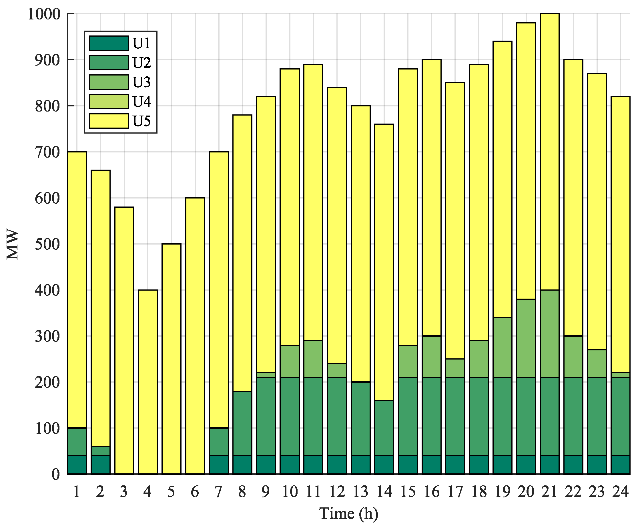
Figure 2 is a graphic representation of the optimal solution. Unit commitment without transmission network constraints is solved, and the optimal cost is $229,700. This schedule makes extensive use of the Units 1, 2, and 5 (U1, U2, and U5), but it does not use Unit 4 (U4) at all. U1 reaches its upper limit of generation during all its online periods because it is the cheapest unit; i.e., it is dispatched to generate as much power as often as possible.

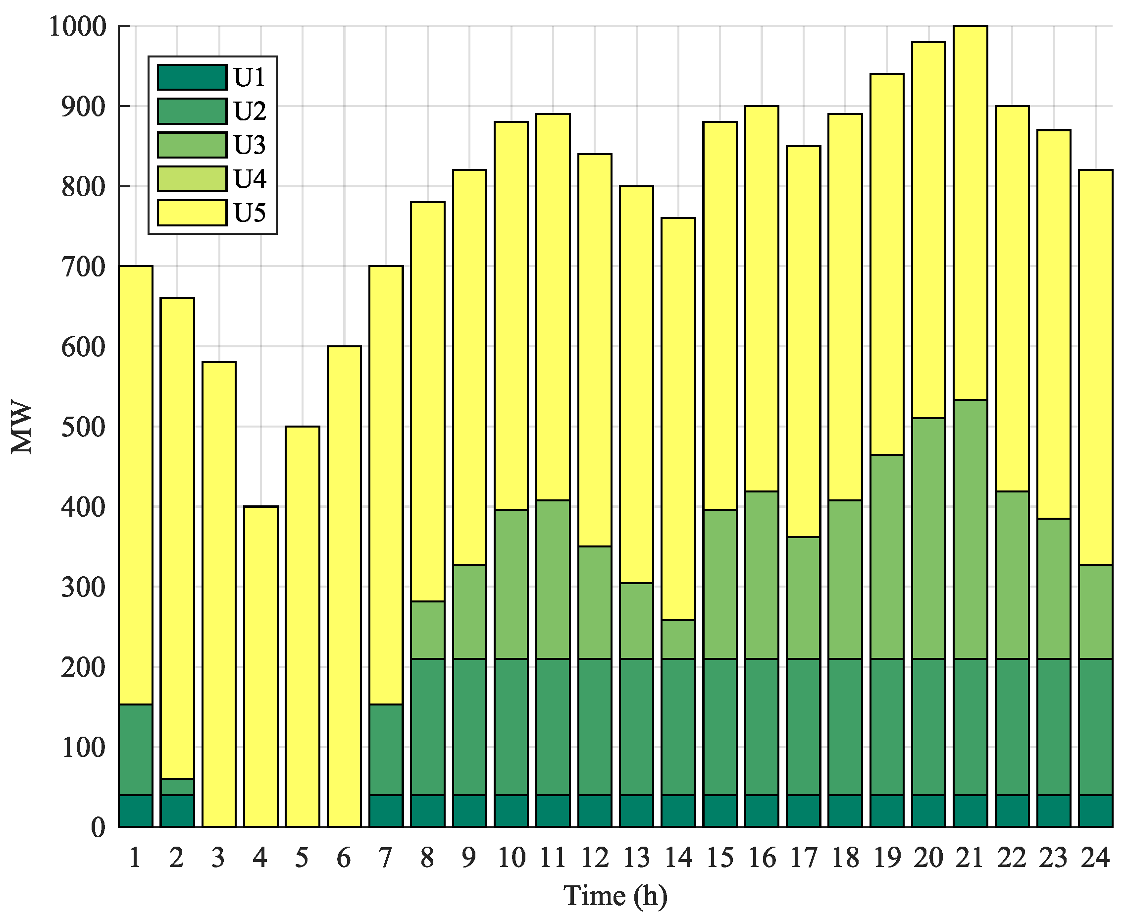
Figure 3 displays the UC scheduling and hourly output power generation. For this optimization problem, there is congestion in transmission line between bus D and E during almost all of the 24-hour period, except from hour 2 to hour 6. These power flows reach their limits since U5 produces as much power as possible, while it is constrained by transmission limits.

Compared the total cost considering both cases, the increased cost due to the transmission network ($267,904.7 − $229,700.0 = $38,204.7) is about 17% of the total cost.

Table 2. Computational aspects of the PJM 5-bus system.

Formulation	DC	PTDF	GGDF
Equality constraints	240	144	144
Inequality constraints	2112	2112	2112
Total constraints	2352	2256	2256
Binary variables	360	360	365
Continuous variables	1296	1200	1200
Total variables	1656	1560	1560
Maximum CPU time (seg)	0.218145	0.218145	0.213139
Minimum CPU time (seg)	0.158108	0.147099	0.145098
Average CPU time (seg)	0.167328	0.156782	0.155799

shows the computational aspects for the three UC models: (1) DC-, (2) PTDF-, and (3) GGDF-based formulations. The DC-based classical formulation requires a larger number of decision variables. With respect to equality constraints, the PTDF- and GGDF-based formulations require (144) constraints, which is much lower than the classical formulation (240). The inequality constraints are the same for all formulations (2112). Comparing the optimal solution with the classical DC- and PTDF-based formulations, it is shown that all solutions are the same, which corroborates the optimality and equivalence of the GGDF-based formulation. It also includes the maximum, minimum, and average simulation time considering 100 trials.

3.2. IEEE 24-Bus Reliability Test System

The IEEE Reliability Test System (RTS) has 33 generating units, 38 transmission lines, and 17 load centers. Bus 1 is selected as the slack bus. The units’ minimum on/off times constraints are taken from [31].

The optimal cost without transmission network constraints is $849,359 for the 24-hour period. The operational constraints such as generation limits, minimum up/down time, and initial status of units are verified. Additionally, there is no unserved energy.

For the next simulation, transmission line 14–16 and transmission line 16–17 are limited to 440 MW. The optimal operational cost is $849,365. For this case, the transmission line 14–16 reaches its limit at only one hour (t = 24), and there is no loss-of-load for any time period.

To compare the performance of the proposed formulation with both the classical DC- and PTDF-based formulations, the line flow limits on lines 14–16 and 16–17 are set to several maximum values. The second and third columns of

Table 3. Impact of congestion on the operational costs.

${\mathit{P}}_{\mathit{m}\mathit{q}}^{\mathit{M}\mathit{a}\mathit{x}} \left(\mathbf{MW}\right)$	Operating Costs ($)	Cost Increment ($)
-	849,359	-
440	849,365	6
420	849,613	254
400	851,880	2521
380	860,470	11,111
360	884,916	35,557
340	919,852	34,936

reports how the operational cost increases caused by the re-dispatch of online units and the commitment of more units in the TCUC problem.

It should be mentioned that the three mathematical formulations obtained the same optimal solution. Therefore, the accuracy and optimality of the GGDF-based formulation is also confirmed. It is worth emphasizing that for all simulations there are not unserved energy and all constraints are verified.

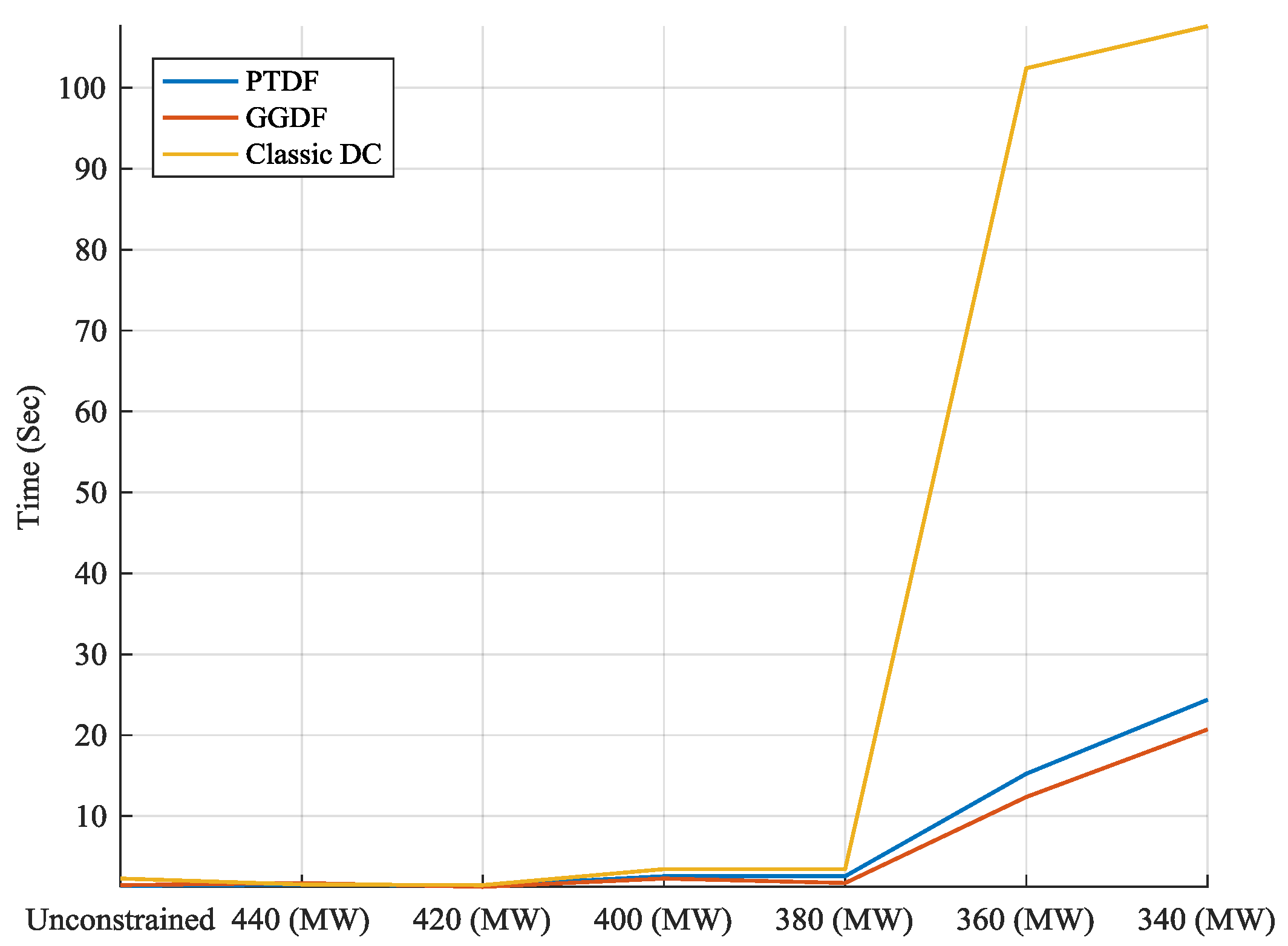
When the transmission limits on lines 14–16 and 16–17 are set to 440 MW, only line 14–16 reaches its limit. However, when the limit is set to 420 MW, line 16–17 also reaches its limit. Line 14–16 operates at its maximum limit for 5 h, and line 16–17 operates at its maximum limit from hour 2 to hour 6. As the transmission limit is reduced, lines 14–16 and 16–17 reach their transmission limits for most of the time. When the limit is set to 360 MW, line 14–16 reaches its limit for the 24 h and line 16–17 from hour 1 to hour 8 and at hour 24.

Figure 4 shows that all formulations require more simulation time to determine the optimization problem as the limit of the transmission network is constrained. In other words, the simulation time increases more than five times for the classical DC-based formulation compared with the PTDF- and GGDF-based formulations, when, for example, the transmission power flow constraint is set to 360 MW.

3.3. IEEE 118-Bus System

The IEEE 118-bus test system has 91 buses with loads, 186 existing branches, and 54 generators. Bus 69 is selected as the slack bus. The system and production cost data are taken from [31].

Table 4. Computational aspects for the IEEE 118-bus system.

Formulation	DC	PTDF	GGDF
Equality constraints	4128	1320	1320
Inequality constraints	28,392	28,392	28,392
Total constraints	32,520	29,712	29,712
Binary variables	3888	3888	3888
Continuous variables	15,768	12,960	12,960
Total variables	19,656	16,848	16,848

shows that the number of inequality constraints in the classical DC formulation is 4128, whereas the number of equality constraints is 1320 for the PTDF- and GGDF-based formulations. The number of decision variables for the classical formulation is 19,656, whereas the number of decision variables is 16,848 for both (PTDF and GGDF) formulations.

Considering the lower simulation time obtained by the GGDF-based formulation, we will use this methodology to evaluate the transmission-constrained UC problem using different transmission network conditions.

The optimal cost without the transmission network constraints is $2,246,477 for the 24-hour period.

Table 5. Impact of congestion on operating costs.

${\mathit{P}}_{\mathit{m}\mathit{q}}^{\mathit{M}\mathit{a}\mathit{x}} \left(\mathbf{MW}\right)$	Operational Costs ($)	Cost Increment ($)
-	2,246,477	-
420	2,246,510	33
380	2,246,675	165
340	2,247,515	840
300	2,249,704	2189
260	2,253,259	3555
240	2,259,500	11,985
180	2,273,226	13,726
140	2,300,779	27,553

reports the impact of congestion in the operational costs for different maximum power flow limits assuming that all transmission lines are limited to the set value. As expected, operational costs increase for each reduction in the maximum power flow limit.

To investigate the GGDF’s computational performance, we increase the time period horizon from one day to one week using the same daily system load for every day. In this case, the optimal cost is $15,725,340, and the CPU execution time for solving the proposed UC formulation is 9.6250 sec.

4. Conclusions

This paper presented an alternative formulation to take into account the transmission network constraints in the UC problem. The GGDF-based formulation, similar to the PTDF-based formulation, required fewer variables because it excluded the voltage phase angles as decision variables. The accuracy and performance in the transmission-constrained UC problem using the GGDF-based formulation were compared with the classical DC- and PTDF-based formulations using several test electrical power systems (PJM 5-bus system, IEEE 24-bus RTS system, and IEEE 118-bus system). Simulations accomplished in this study using a commercial solver support the accuracy and superior computational performance of the proposed formulation, with results showing that it can lead to a more suitable methodology applied especially to medium and large-scale electrical power systems without sacrificing optimality.

Future work will incorporate uncertainty in the proposed transmission-constrained UC problem described in this paper. Modeling renewable uncertainty and decomposition techniques (Benders) will also be studied soon.

References

- O’Neill, R.P.; Helman, U.; Sotkiewicz, P.M.; Rothkopf, M.H.; Stewart, W.R. Regulatory Evolution, Market Design and Unit Commitment. In The Next Generation of Electric Power Unit Commitment Models; Hobbs, B.F., Rothkopf, M.H., O’Neill, R.P., Chao, H., Eds.; Springer: Boston, MA, USA; Volume 36, pp. 15–37.
- Inostroza, J.; Hinojosa, V.H. Short-term scheduling solved with a particle swarm optimizer. IET Gener. Transm. Distrib. 2011, 5, 1091–1104. [Google Scholar] [CrossRef]
- Fu, Y.; Li, Z.; Wu, L. Modeling and solution of the large-scale security-constrained unit commitment. IEEE Trans. Power Syst. 2013, 28, 3524–3533. [Google Scholar] [CrossRef]
- Fu, Y.; Shahidehpour, M. Fast SCUC for large-scale power systems. IEEE Trans. Power Syst. 2007, 22, 2144–2151. [Google Scholar] [CrossRef]
- Khodaei, A.; Shahidehpour, M. Transmission switching in security-constrained unit commitment. IEEE Trans. Power Syst. 2010, 25, 1937–1945. [Google Scholar] [CrossRef]
- Ostrowski, J.; Wang, J. Network reduction in the transmission-constrained unit commitment problem. Comput. Ind. Eng. 2012, 63, 702–707. [Google Scholar] [CrossRef]
- Pandzic, H.; Qiu, T.; Kirschen, D.S. Comparison of State-of-the-Art Transmission Constrained Unit Commitment Formulations. In Proceedings of the 2013 IEEE Power and Energy Society General Meeting, Vancouver, BC, Canada, 21–25 July 2013. [Google Scholar]
- Sahebi, M.M.R.; Hosseini, S.H. Stochastic security constrained unit commitment incorporating demand side reserve. Int. J. Electr. Power Energy Syst. 2014, 56, 175–184. [Google Scholar] [CrossRef]
- Wang, F.; Hedman, K.W. Dynamic reserve zones for day-ahead unit commitment with renewable resources. IEEE Trans. Power Syst. 2015, 30, 612–620. [Google Scholar] [CrossRef]
- Nasrolahpour, E.; Ghasemi, H. A stochastic security constrained unit commitment model for reconfigurable networks with high wind power penetration. Electric Power Syst. Res. 2015, 121, 341–350. [Google Scholar] [CrossRef]
- Li, Z.; Wu, W.; Wang, J.; Zhang, B.; Zheng, T. Transmission-Constrained unit commitment considering combined electricity and district heating networks. IEEE Trans. Sustain. Energy 2016, 7, 480–492. [Google Scholar] [CrossRef]
- Hinojosa-Mateus, V.; Gutiérrez-Alcaraz, G. A computational comparison of 2 mathematical formulations to handle transmission network constraints in the unit commitment problem. Int. Trans. Electr. Energy Syst. 2017, 27, 1–15. [Google Scholar]
- Alvarez, G.E.; Marcovecchio, M.G.; Aguirre, P.A. Security-Constrained unit commitment problem including thermal and pumped storage units: An MILP formulation by the application of linear approximations techniques. Electr. Power Syst. Res. 2018, 154, 67–74. [Google Scholar] [CrossRef]
- Shaw, J.J. A direct method for security-constrained unit commitment. IEEE Trans. on Power Syst. 1995, 10, 1329–1342. [Google Scholar] [CrossRef]
- Ma, H.; Shahidehpour, S.M. Transmission-constrained unit commitment based on Benders decomposition. Electr. Power Energy Syst. 1998, 20, 287–294. [Google Scholar] [CrossRef]
- Tseng, C.-L.; Oren, S.S.; Cheng, C.S.; Li, C.; Svoboda, A.J.; Johnson, R.B. A transmission-constrained unit commitment method in power system scheduling. Decis. Support Syst. 1999, 24, 297–310. [Google Scholar] [CrossRef]
- Kalantari, A.; Restrepo, J.F.; Galiana, F.D. Security-constrained unit commitment with uncertain wind generation: The loadability set approach. IEEE Trans. on Power Syst. 2013, 28, 1787–1796. [Google Scholar] [CrossRef]
- Helseth, A.; Warland, G.; Mo, B. A hydrothermal market model for simulation of area prices including detailed network analyses. Int. Trans. Electr. Energ. Syst. 2013, 23, 1396–1408. [Google Scholar] [CrossRef]
- Hu, B.; Wu, L.; Marwali, M. On the robust solution to SCUC with load and wind uncertainty correlations. IEEE Trans. Power Syst. 2014, 29, 2952–2964. [Google Scholar] [CrossRef]
- Morales-España, G.; Baldick, R.; García-González, J.; Ramos, A. Power-capacity and ramp-capability reserves for wind integration in power-based UC. IEEE Trans. Sustain. Energy 2016, 7, 614–624. [Google Scholar]
- Tejada-Arango, D.A.; Sánchez-Martın, P.; Ramos, A. Security constrained unit commitment using line outage distribution factors. IEEE Trans. Power Syst. 2018, 33, 329–337. [Google Scholar] [CrossRef]
- Ng, W.Y. Generalized generation distribution factors for power system security evaluations. IEEE Trans. Power Appar. Syst. 1981, 3, 1001–1005. [Google Scholar] [CrossRef]
- Zhang, H.; Vittal, V.; Heydt, G.T.; Quintero, J. Mixed-Integer Linear Programming approach for multi-stage security-constrained transmission expansion planning. IEEE Trans. Power Appar. Syst. 2012, 27, 1125–1133. [Google Scholar] [CrossRef]
- Hinojosa, V.; Ticuna, O.; Gutierrez, G. Improving the mathematical formulation of the unit commitment with transmission system constraints. IEEE Latin Am. Trans. 2016, 14, 773–781. [Google Scholar] [CrossRef]
- Hinojosa, V.H.; Gonzales-Longatt, F. Preventive security-constrained DC-OPF formulation using power transmission distribution factors and line outage distribution factors. Energies 2018, 11, 1497. [Google Scholar] [CrossRef]
- Hinojosa, V.H. A generalized stochastic N-m security-constrained generation expansion planning methodology using partial transmission distribution factors. In Proceedings of the IEEE Power and Energy Society General Meeting Conference 2017, Chicago, IL, USA, 16–20 July 2017. [Google Scholar]
- Matpower. Available online: http:// www.pserc.cornell.edu/matpower (accessed on 18 August 2018).
- Arroyo, J.M.; Conejo, A.J. Optimal response of a thermal unit to an electricity spot market. IEEE Trans. Power Syst. 2000, 15, 1098–1104. [Google Scholar] [CrossRef]
- Li, F.; Bo, R. Small test systems for power system economic studies. In Proceedings of the IEEE Power and Energy Society General Meeting, Providence, RI, USA, 25–29 July 2010; pp. 1–4. [Google Scholar]
- Grigg, C.; Wong, P.; Albrecht, P.; Allan, R.; Bhavaraju, M.; Billinton, R.; Chen, Q.; Fong, C.; Haddad, S.; Kuruganty, S.; et al. The IEEE reliability test system—1996. A report prepared by the reliability test system task force of the application of probability methods subcommittee. IEEE Trans. power syst. 1999, 14, 1010–1020. [Google Scholar] [CrossRef]
- The REAL Lab Library. University of Washington, Department of Electrical Engineering. Available online: http://www.ee.washington.edu/research/real/library.html (accessed on 18 August 2018).
Figure 1.
The PJM 5-bus system.
Figure 2.
Units’ output power without transmission congestion.
Figure 3.
Units’ output power with transmission congestion.
Figure 4.
Average run times of TCUC with different transmission network limits.