Experimental Study on the Performance of Controllers for the Hydrogen Gas Production Demanded by an Internal Combustion Engine

 , ,
, ,
Abstract
:1. Introduction
2. Materials and Method
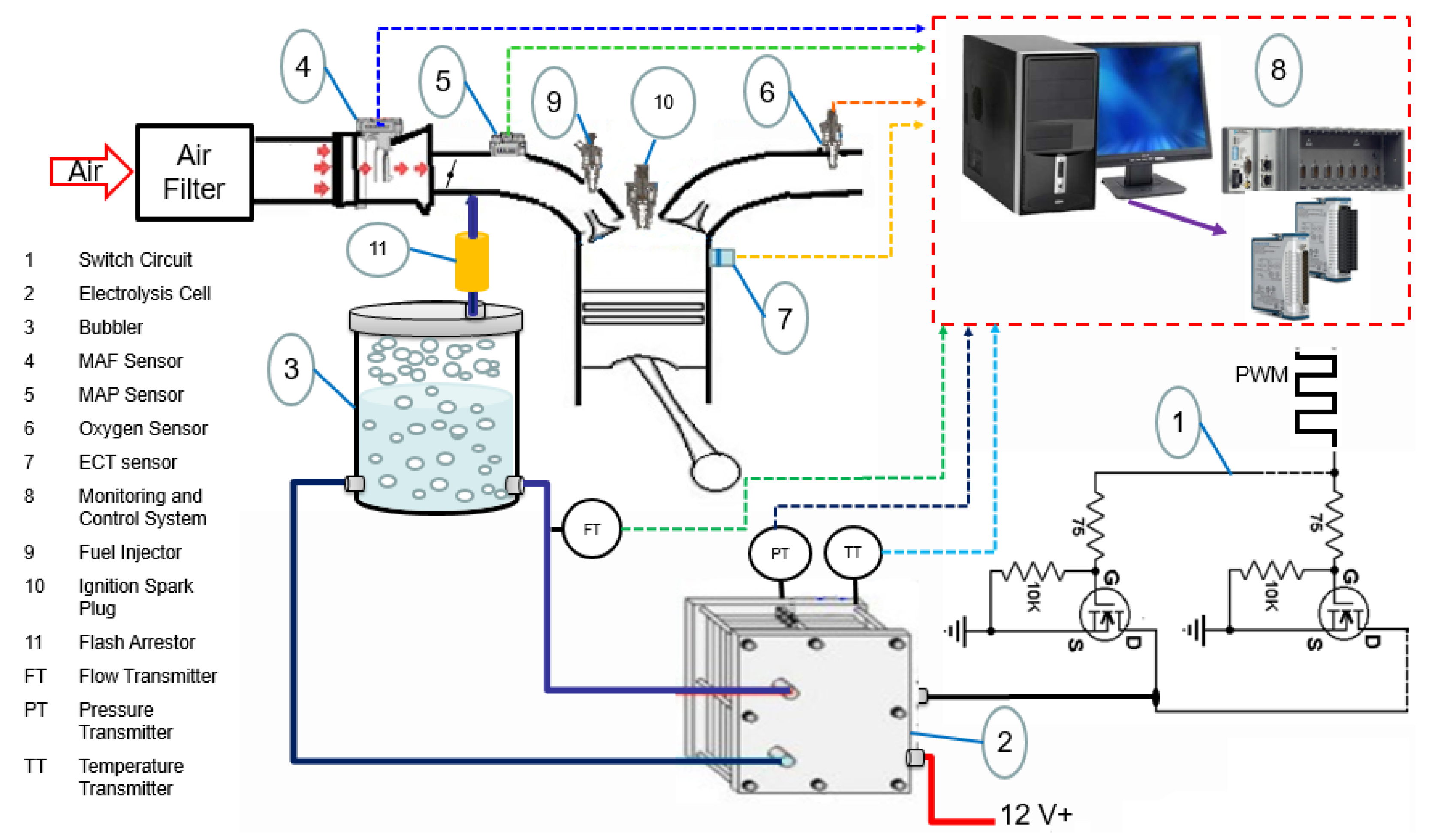
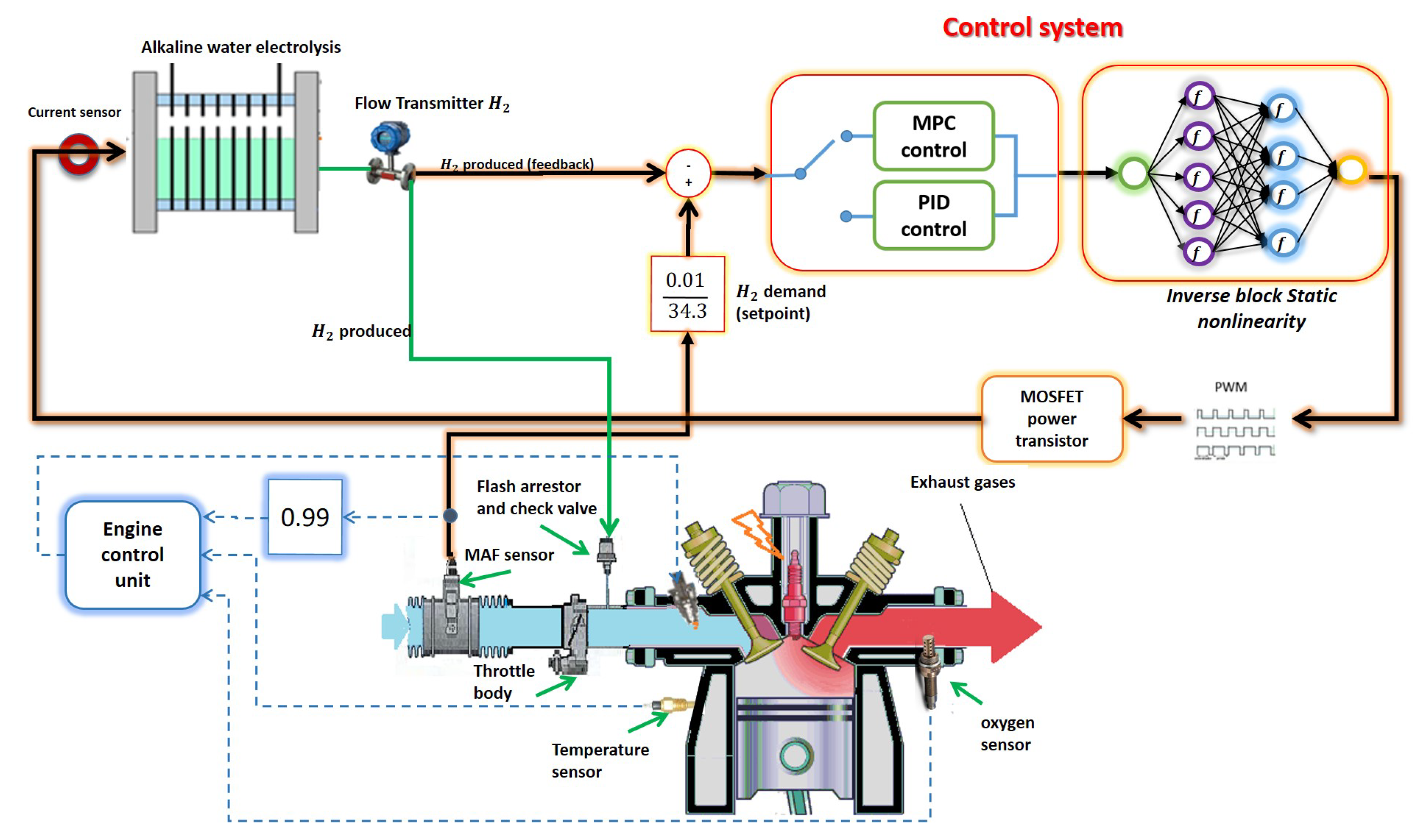
2.1. Instrumentation, Sensors and Acquisition System
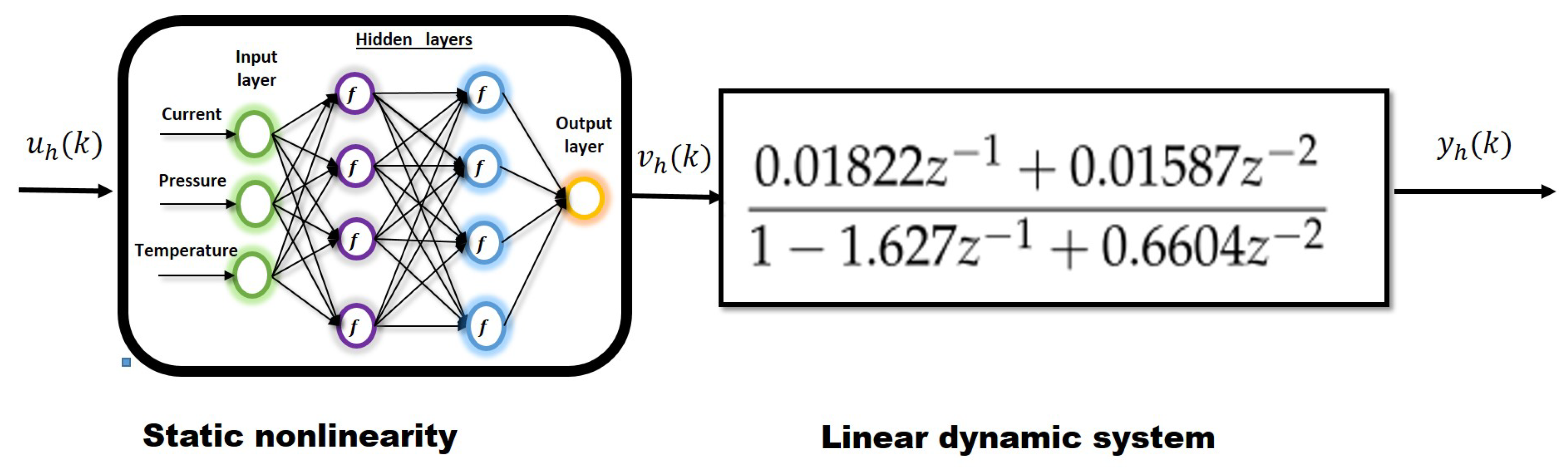
2.2. Nonlinear Identification Hammerstein Models
2.3. Model Predictive Control Law
2.4. Proportional Integral Derivative Control Law
PID Tuning
2.5. Engine Efficiencies
2.6. Control Strategy
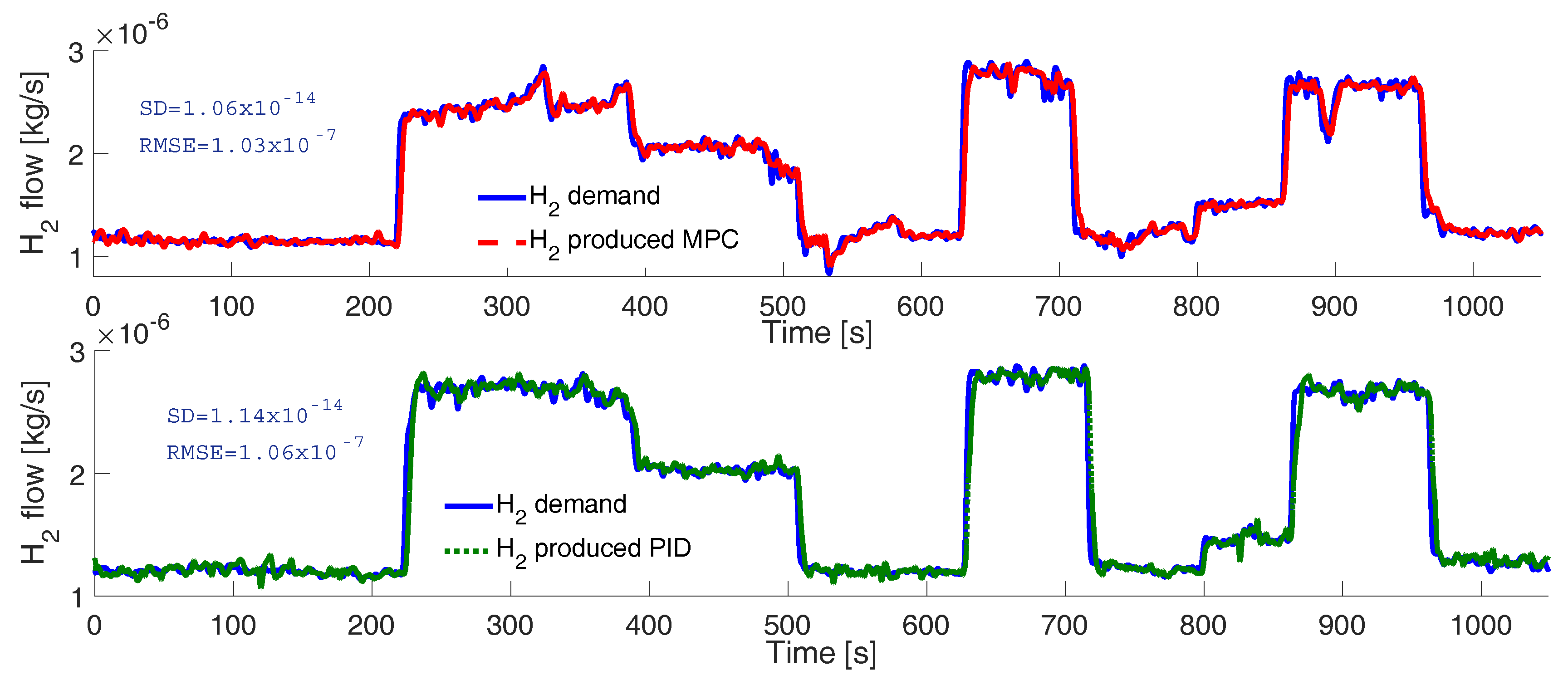
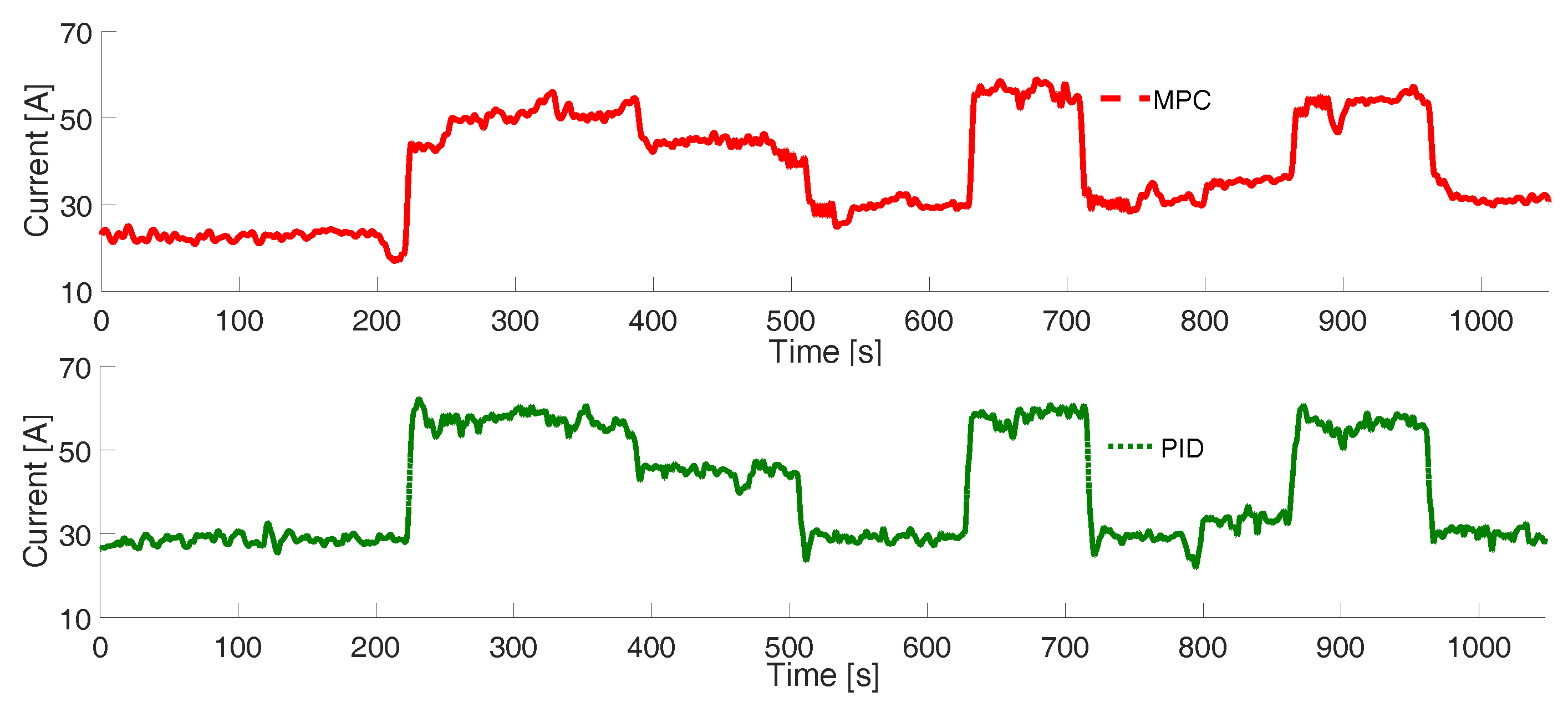
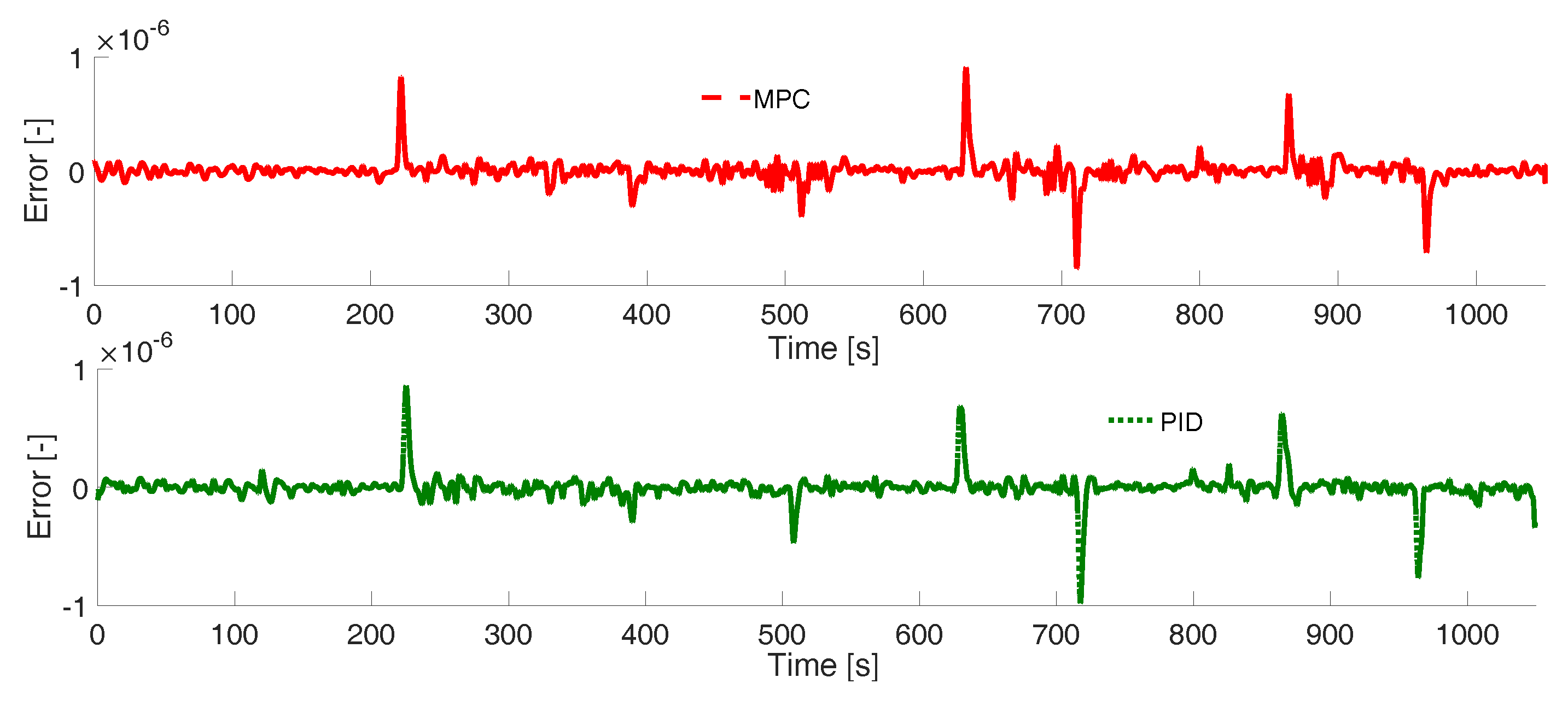
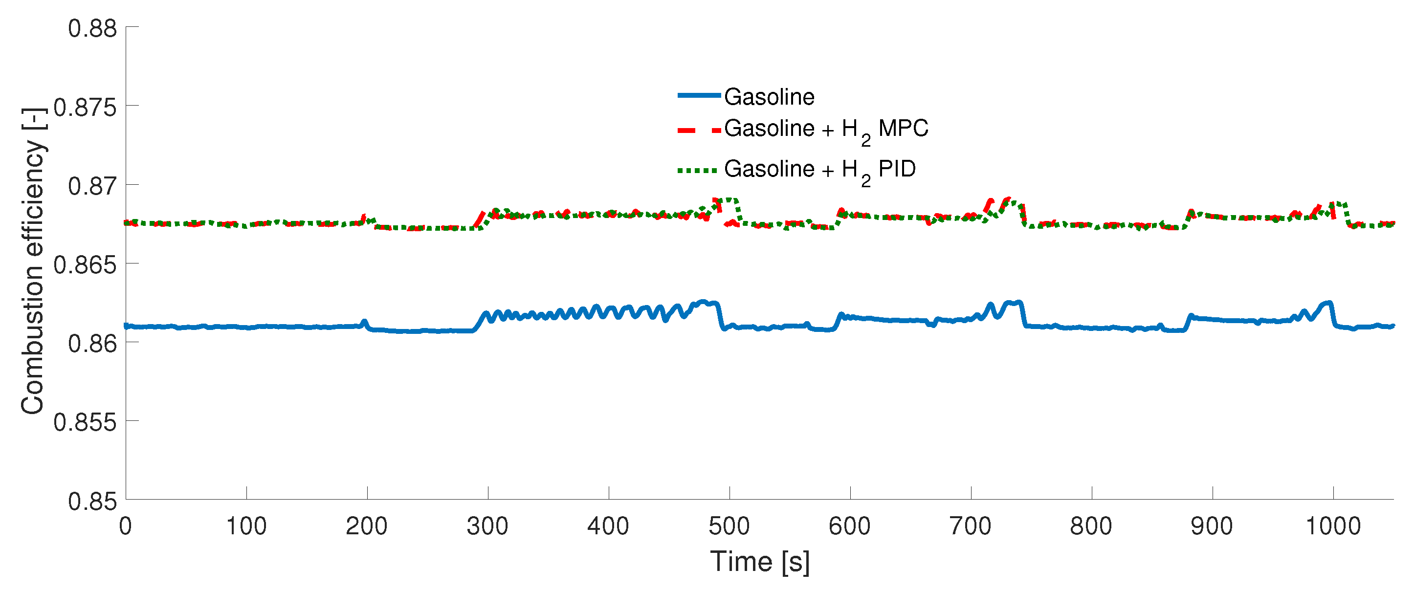
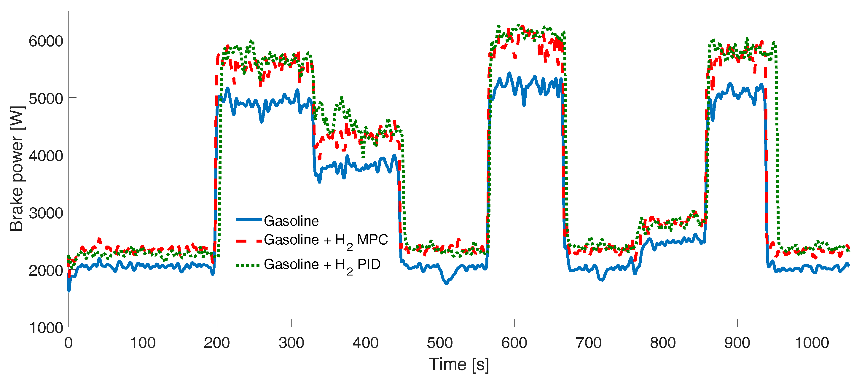
3. Results
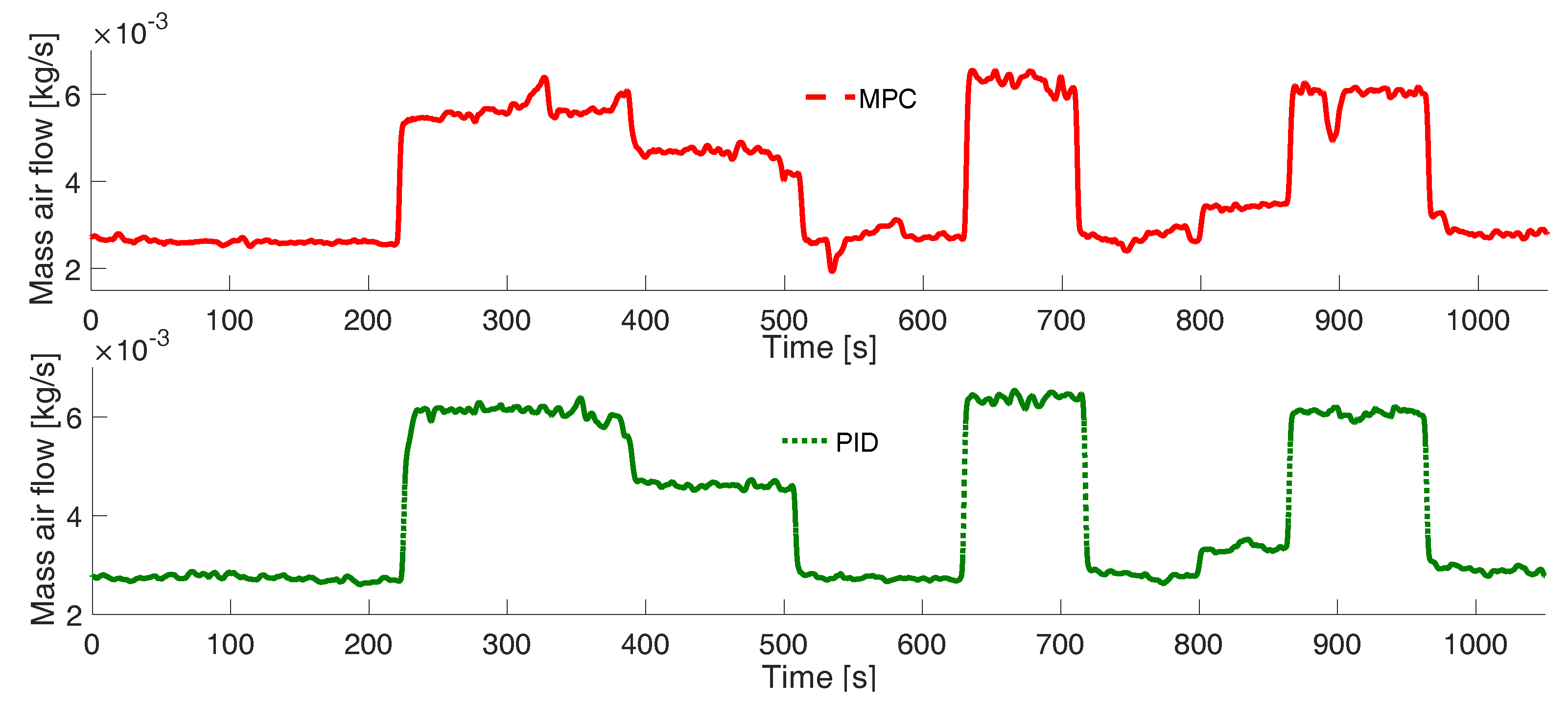
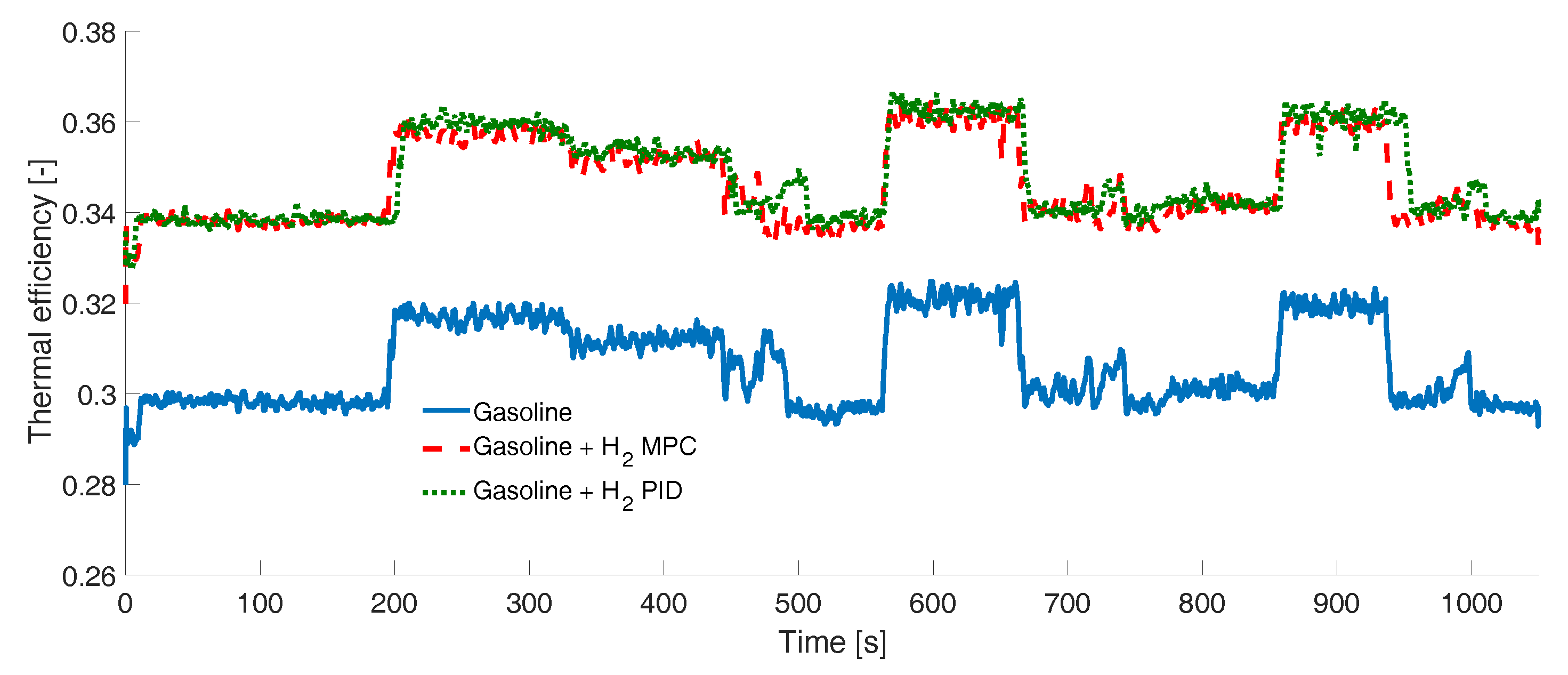
Experimental Tests
4. Conclusions
Author Contributions
Funding
Acknowledgments
Conflicts of Interest
Nomenclature
| Acronyms | |
| Air/Fuel Ratio | |
| Stoichiometric Air/Fuel Ratio | |
| ANN | Artificial Neural Network |
| Auto Regressive with eXogenous inputs | |
| MPC | Model Predictive Control |
| PID | Proportional Integral Derivative |
| PWM | Pulse-Width Modulation |
| SD | Standard deviation |
| SLM | Standard Litre per Minute |
| Root mean square error | |
| RTD | Resistance Temperature Detector |
| Symbols | |
| Factor for determining the third pole | |
| State-space realization | |
| u | Future input change |
| Damping factor | |
| J | Performance index for optimization CMPC |
| Pair of matrices used in the prediction equation | |
| Factor indicating whether the mixture is rich or lean | |
| Combustion efficiency | |
| Thermal efficiency | |
| Volumetric efficiency | |
| Natural frequency | |
| Model Hammerstein Output | |
| Model articial neural network | |
| Constants | |
| Control horizon | |
| Prediction horizon |
References
- Ji, C.; Wang, S. Combustion and emissions performance of a hybrid hydrogen–gasoline engine at idle and lean conditions. Int. J. Hydrogen Energy 2010, 35, 346–355. [Google Scholar] [CrossRef]
- Al-Rousan, A.A. Reduction of fuel consumption in gasoline engines by introducing HHO gas into intake manifold. Int. J. Hydrogen Energy 2010, 35, 12930–12935. [Google Scholar] [CrossRef]
- Karagöz, Y.; Orak, E.; Yüksek, L.; Sandalcı, T. Effect of hydrogen addition on exhaust emissions and performance of a spark ignition engine. Environ. Eng. Manag. J. 2015, 14, 665–672. [Google Scholar] [CrossRef]
- Tzimas, E.; Filiou, C.; Peteves, S.D.; Veyret, J.B. Hydrogen Storage: State-of-the-Art and Future Perspective; EUR-Scientific and Technical Research Reports; EU Commission, JRC Petten, EUR 20995EN: Petten, The Netherlands, 2003. [Google Scholar]
- Dahbi, S.; Aboutni, R.; Aziz, A.; Benazzi, N.; Elhafyani, M.; Kassmi, K. Optimised hydrogen production by a photovoltaic-electrolysis system DC/DC converter and water flow controller. Int. J. Hydrogen Energy 2016, 41, 20858–20866. [Google Scholar] [CrossRef]
- Sandeep, K.C.; Kamath, S.; Mistry, K.; Kumar, A.; Bhattacharya, S.K.; Bhanja, K.; Mohan, S. Experimental studies and modeling of advanced alkaline water electrolyser with porous nickel electrodes for hydrogen production. Int. J. Hydrogen Energy 2017, 42, 12094–12103. [Google Scholar] [CrossRef]
- Haug, P.; Kreitz, B.; Koj, M.; Turek, T. Process modelling of an alkaline water electrolyzer. Int. J. Hydrogen Energy 2017, 42, 15689–15707. [Google Scholar] [CrossRef]
- Olivier, P.; Bourasseau, C.; Bouamama, P.B. Low-temperature electrolysis system modelling: A review. Renew. Sustain. Energ. Rev. 2017, 78, 280–300. [Google Scholar] [CrossRef]
- Dixon, C.; Reynolds, S.; Rodley, D. Micro/small wind turbine power control for electrolysis applications. Renew. Energy 2016, 87, 182–192. [Google Scholar] [CrossRef]
- Bhattacharyya, R.; Misra, A.; Sandeep, K.C. Photovoltaic solar energy conversion for hydrogen production by alkaline water electrolysis: conceptual design and analysis. Energy Convers. Manag. 2017, 133, 1–13. [Google Scholar] [CrossRef]
- Aguilar, J.V.; Langarita, P.; Rodellar, J.; Linares, L.; Horváth, K. Predictive control of irrigation canals-robust design and real-time implementation. Water Resour. Manag. 2016, 11, 3829–3843. [Google Scholar] [CrossRef]
- Serna, Á.; Yahyaoui, I.; Normey-Rico, J.E.; de Prada, C.; Tadeo, F. Predictive control for hydrogen production by electrolysis in an offshore platform using renewable energies. Int. J. Hydrogen Energy 2017, 42, 12865–12876. [Google Scholar] [CrossRef] [Green Version]
- Eskinat, E.; Johnson, S.H.; Luyben, W.L. Use of hammerstein models in identification of nonlinear systems. AIChE J. 1991, 37, 255–268. [Google Scholar] [CrossRef]
- Wang, L. Model Predictive Control System Design and Implementation Using MATLAB; Springer: London, UK, 2009. [Google Scholar]
- Persson, P.; Åström, K.J. PID control revisited. IFAC Proc. Vol. 1993, 26, 451–454. [Google Scholar] [CrossRef]
- Åström, K.J.; Hägglund, T. PID Controllers: Theory, Design, and Tuning; International Society of Automation: Research Triangle Park, NC, USA, 1995. [Google Scholar]
- Hendricks, E.; Sorenson, S.C. Mean value modelling of spark ignition engines. J. Egines 1990, 99, 1359–1373. [Google Scholar]
- Blair, G.P. Design and Simulation of Two-Stroke Engines; Society of Automotive Engineers: Warrendale, PA, USA, 1996. [Google Scholar]
- Hacohen, Y.; Sher, E. Fuel consumption and emission of SI engine fueled with H/sub 2/-enriched gasoline. In Proceedings of the 24th Intersociety Energy Conversion Engineering Conference, Washington, DC, USA, 6–11 August 1989. [Google Scholar]
- Amrouche, A.; Erickson, P.A.; Varnhagen, S.; Park, J.W. An experimental study of a hydrogen-enriched ethanol fueled Wankel rotary engine at ultra lean and full load conditions. Energy Convers. Manag. 2016, 123, 174–184. [Google Scholar] [CrossRef]


| IC Engine Characteristic | Value |
|---|---|
| Number of cylinders | 4 |
| Cylinder displacement volumetric | 1.595 l |
| Ratio of cylinder bore to piston stroke | 0.863 |
| Compression ratio | 9.5:1 |
| Maximum power | 78 kW/6000 rpm |
| Maximum torque | 138 Nm/4000 rpm |
| Minimum regime | 625 rpm |
| Maximum regime | 6000 rpm |
| Valves | 4 valves/cylinder |
| Throttle radio | 50 mm |
| Manifold volume | 0.00148 m |
| ANN Model | Wi | 0.6125 | 0.3984 | 1.2064 | −0.0551 | |
| (k,j) | (1,1) | (1,2) | (1,3) | (1,4) | ||
| 0.8307 | 0.5240 | 0.1781 | 0.4856 | |||
| (2,1) | (2,2) | (2,3) | (2,4) | |||
| 0.3771 | 0.4739 | 0.1599 | 0.2283 | |||
| (3,1) | (3,2) | (3,3) | (3,4) | |||
| Wl | 0.6006 | −0.5282 | 0.5764 | 0.1417 | ||
| (j,p) | (1,1) | (1,2) | (1,3) | (1,4) | ||
| 0.5839 | 0.5730 | 0.2632 | 0.4318 | |||
| (2,1) | (2,2) | (2,3) | (2,4) | |||
| 0.6206 | −1.8939 | 1.1354 | 0.1056 | |||
| (3,1) | (3,2) | (3,3) | (3,4) | |||
| 0.4143 | 1.3315 | −0.3020 | 0.3203 | |||
| (4,1) | (4,2) | (4,3) | (4,4) | |||
| Wo | 1.3432 | −4.1812 | 2.0479 | 0.3280 | ||
| (p,i) | (1,1) | (2,1) | (3,1) | (4,1) | ||
| ANN Model of the Inverse Block | Wi | 0.5808 | −0.4829 | 1.0060 | 0.1710 | 1.0027 |
| (k,j) | (1,1) | (1,2) | (1,3) | (1,4) | (1,5) | |
| Wl | 0.0960 | 0.1391 | 0.3053 | 0.1893 | ||
| (j,p) | (1,1) | (1,2) | (1,3) | (1,4) | ||
| −0.4767 | 0.0118 | −0.9156 | 1.9820 | |||
| (2,1) | (2,2) | (2,3) | (2,4) | |||
| 1.0418 | 0.6608 | 0.9554 | −1.3087 | |||
| (3,1) | (3,2) | (3,3) | (3,4) | |||
| −0.1652 | 0.3466 | 0.0727 | 0.7675 | |||
| (4,1) | (4,2) | (4,3) | (4,4) | |||
| 0.8474 | 0.6595 | 0.7353 | −1.0418 | |||
| (5,1) | (5,2) | (5,3) | (5,4) | |||
| Wo | 1.4605 | 0.6381 | 1.5800 | −3.2777 | ||
| (p,i) | (1,1) | (2,1) | (3,1) | (4,1) |
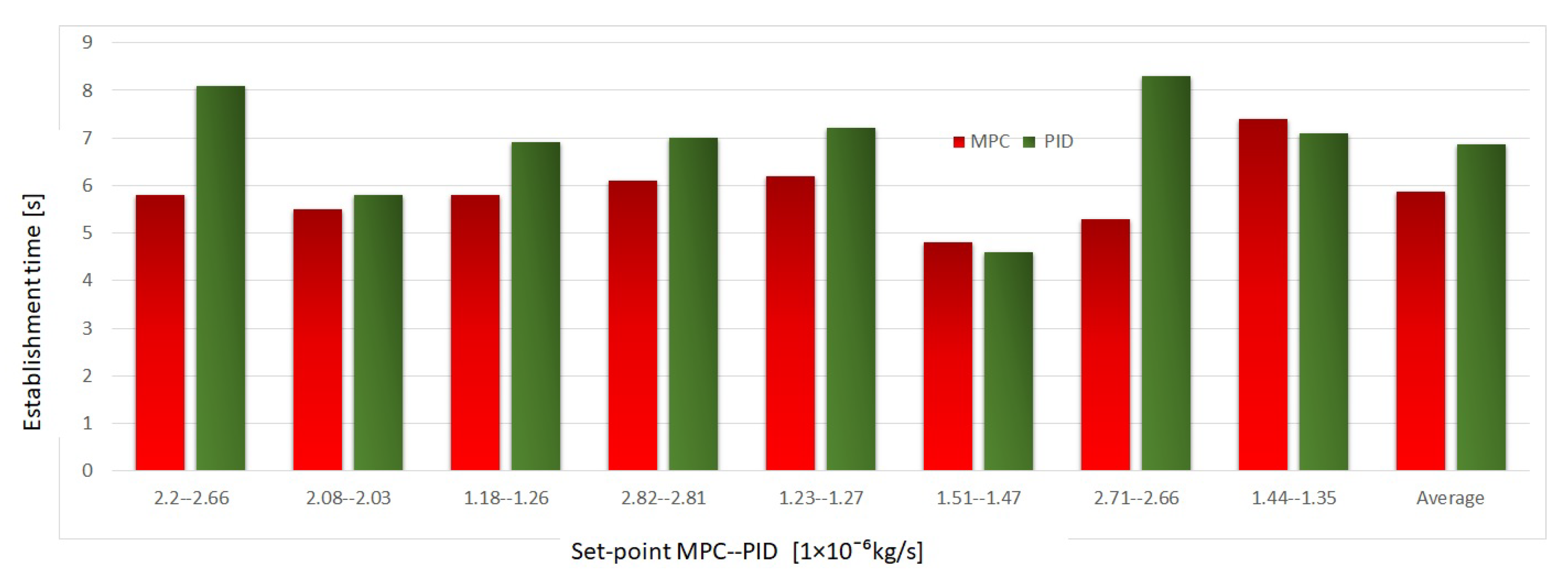
| Setpoint MPC–PID ( kg/s) | Establishment Time MPC (s) | Establishment Time PID (s) |
|---|---|---|
| 2.20–2.66 | 5.8 | 8.1 |
| 2.08–2.03 | 5.5 | 5.8 |
| 1.18–1.26 | 5.8 | 6.9 |
| 2.82–2.81 | 6.1 | 7.0 |
| 1.23–1.27 | 6.2 | 7.1 |
| 1.51–1.47 | 4.8 | 4.6 |
| 2.71–2.66 | 5.3 | 8.3 |
| 1.44–1.35 | 7.4 | 7.1 |
| Average | 5.8 | 6.8 |
© 2018 by the authors. Licensee MDPI, Basel, Switzerland. This article is an open access article distributed under the terms and conditions of the Creative Commons Attribution (CC BY) license (http://creativecommons.org/licenses/by/4.0/).
Share and Cite
Cervantes-Bobadilla, M.; Escobar-Jiménez, R.F.; Gómez-Aguilar, J.F.; García-Morales, J.; Olivares-Peregrino, V.H. Experimental Study on the Performance of Controllers for the Hydrogen Gas Production Demanded by an Internal Combustion Engine. Energies 2018, 11, 2157. https://doi.org/10.3390/en11082157
Cervantes-Bobadilla M, Escobar-Jiménez RF, Gómez-Aguilar JF, García-Morales J, Olivares-Peregrino VH. Experimental Study on the Performance of Controllers for the Hydrogen Gas Production Demanded by an Internal Combustion Engine. Energies. 2018; 11(8):2157. https://doi.org/10.3390/en11082157
Chicago/Turabian StyleCervantes-Bobadilla, Marisol, Ricardo Fabricio Escobar-Jiménez, José Francisco Gómez-Aguilar, Jarniel García-Morales, and Víctor Hugo Olivares-Peregrino. 2018. "Experimental Study on the Performance of Controllers for the Hydrogen Gas Production Demanded by an Internal Combustion Engine" Energies 11, no. 8: 2157. https://doi.org/10.3390/en11082157