Carbon Taxes and Carbon Right Costs Analysis for the Tire Industry

Department of Business Administration, National Central University, Jhongli, Taoyuan 32001, Taiwan
Energies 2018, 11(8), 2121; https://doi.org/10.3390/en11082121
Submission received: 4 July 2018
/
Revised: 31 July 2018
/
Accepted: 9 August 2018
/
Published: 14 August 2018
(This article belongs to the Special Issue Modeling and Simulation of Carbon Emission Related Issues)
Abstract
:As enterprises are the major perpetrators of global climate change, concerns about global warming, climate change, and global greenhouse gas emissions continue to attract attention, and have become international concerns. The tire industry, which is a high-pollution, high-carbon emission industry, is facing pressure to reduce its carbon emissions. Thus, carbon prices and carbon trading have become issues of global importance. In order to solve this environmental problem, the purpose of this paper is to combine mathematical programming, Theory of Constraints (TOC), and Activity-Based Costing (ABC) to formulate the green production decision model with carbon taxes and carbon right costs, in order to achieve the optimal product mix decision under various constraints. This study proposes three different scenario models with carbon taxes and carbon right used to evaluate the effect on profit of changes in carbon tax rates.
1. Introduction
The international community has paid considerable attention to environmental protection in recent years. Carbon taxes are considered as effective tools to curb greenhouse gas emissions. Analysis of the empirical evidence of carbon tax benefits, including indirect effects on technological developments and other pollutants (i.e., co-benefits) also added suppliers to improve energy price expectations in the future, and empirically propose the first green research contribution [1] and the United Nations has successively enacted relevant laws and regulations, such as the international Greenhouse Gas Emission Act and the 2015 Paris Accord [2], in the hope that the environment we live in will not continue to deteriorate. Due to high technology and industrial development, anthropocentric greenhouse gases are continually generated and accumulate, leading to increased global warming, and deteriorating climate and environmental ecology. In the past decade, it has been well recognized that environmental and economic performance are mutually reinforcing, with improved environmental performance leading to lower costs, increased sales, and greater economic efficiency. That joint effects will help companies to obtain temporary financing and minimize the damage to the environment stemming from carbon emissions [3]. Different perspectives and empirical studies [4] suggest that more attention should be paid to the causal relationship between eco-efficiency and different environmental management approaches, as well as their economic consequences; for example, the implementation of a carbon tax will help to improve the environment, promoting carbon taxes as a policy to improve the cost-effectiveness of carbon emissions. However, in the current practice of environmental policy, only a few countries implement taxation based on carbon content. According to empirical results, the carbon tax may be an interesting policy choice, and the negative impact can be compensated by designing taxes and the fiscal revenue generated by the use [5]. Various environmental policy tools are used in critical assessment criteria, including cost-effectiveness, equitable distribution, risk minimization of uncertainty and political feasibility. Additional considerations include carbon taxes, tradable emission allowances, emission reduction subsidies, and research and development subsidies [6]. In the actual situation of the EU, the implementation of the carbon price policy can achieve the goal of emission reduction, and the carbon trading results also show that carbon emissions can be controlled through carbon trading [7]. But when the regulatory company gets compensation, efficiency needs to be paid among the companies to balance the damage caused by the marginal probability. Applying this basic economic logic to the analysis of the compensation rules proposed under the EU Emissions Trading Scheme, emissions permits can be allocated free of charge to carbon-intensive and trade-exposed industries [8]. However, various environmental policy instruments, including carbon emission taxes, tradable emission allowances, emission reduction subsidies, performance standards, technical tasks, and research and development subsidies, can meet major evaluation criteria, including cost-effectiveness, fair distribution, and risk minimization of uncertainty, and political feasibility [9]. Investigating carbon prices in China, the results show that it has important policy implications for regional markets to be included in national carbon trading [10]. The impact of the Emissions Trading Scheme (ETS) is one of the most effective mitigation measures [11]. The tire industry’s production process greatly increases atmospheric greenhouse gas concentrations. At present, many countries have adopted a “carbon tax” levy to solve corporate carbon emission problems with the related costs borne by enterprises. Sathre and Gustavsson believed that taxation on environmental issues can reduce pollution [12]. Therefore, the impact of carbon pricing policies on the economy is very significant [13]. In Australia, the carbon premium has become higher and higher after the implementation of the carbon tax, and indicates that a stable long-term policy is needed in the future to enable the carbon pricing mechanism to play its full role [14]. Therefore, the carbon price and carbon trading policy results discussed by the aforementioned research institutes have clearly become the most important issues for governments around the world. In this paper, the carbon taxes and carbon right costs analysis holds only for direct carbon taxes or for cap-and-trade schemes as well through a market determined price for carbon emission allowances.
According to the above research, the effective way to reduce emissions is to implement carbon tax collection and formulate carbon rights trading mechanism. This paper aims to analyze the relevant analysis of carbon emissions in the tire industry. Then the tire industry can employ the Activity-Based Costing (ABC) method and perform related cost calculations. The ABC system provides a means for analyzing non-value-added activity workbooks, such as procedures and production that neglect resource constraints in activity [15,16]. A better solution to the reduction of environmentally harmful products is provided by the Theory of Constraint (TOC) [17,18].
The purpose of this paper is to combine mathematical programming, TOC, and ABC to formulate a green production decision model with carbon taxes and carbon right costs, in order to achieve the optimal product mix decision under various constraints and to analyze the effect on profit of carbon taxes. The tire industry is one of the industries with high pollution and high energy consumption, where its carbon pollution will seriously affect environmental issues [19]. Therefore, further assumes that three different scenario models with carbon taxes and carbon right for tire companies are used for scenario analysis. Hoinka and Ziebik [20] applied mathematical methods to analyze complex energy management systems. In summary this paper will discuss the green ABC production decision-making model. The contribution of this study is that it incorporates the cost of carbon emissions into the mathematical programming, enabling the tire industry to evaluate emissions projects. In recent years, studies on the implementation of carbon trading have provided useful insights and helped to reduce carbon emissions [21,22,23].
2. Research Background
2.1. Carbon Emissions Cost and Carbon Tax
The increasing attention to global warming and climate change has become a common concern among governments around the world; therefore, it is imperative to adopt effective measures to promote energy conservation and carbon reduction, and implement corporate carbon emissions policies. Carbon pricing is a hot topic in climate policy debates. There are still many problems due to numerous reasons for implementing global carbon prices. Therefore, the main arguments for carbon pricing are proposed for analysis and discussion. The relatively low environmental cost of carbon pricing helps to improve the social acceptability of climate policy. This includes correcting the price of property that stimulates rapid environmental innovation. These arguments are underestimated in open debates, where pricing strategies are often overlooked and innovation policy misconceptions are common. However, carbon pricing and technology policies are largely complementary and therefore necessary for effective climate policy. In addition, other tools are used to complement the carbon pricing, and suggestions for solving these problems are proposed. Whether through carbon taxes or carbon emissions trading, reflections on the implementation of global carbon prices, including energy research and innovation research, go beyond the traditional arguments of environmental economics [24].
Due to the abnormal climate change in the world, the impact of air pollution is becoming more and more serious, and people’s health is also seriously threatened. Therefore, effective action must be taken to develop policies to reduce greenhouse gas emissions. People are increasingly concerned about the market instruments in the form of carbon pricing mechanisms. The study found that carbon pricing policies include carbon taxes, limits and transactions, emission reduction credits, clean energy standards and reductions in fossil fuel subsidies. Organize the experience and implementation methods of developing countries. And put forward the carbon pricing applicability for decision-making reference [25]. In South America, a carbon pricing strategy is also proposed for climate issues to cope with environmental pollution problems [26]. Environmental pollution has become a major social and political challenge around the world [27,28], and some studies have yielded positive results. That the application of carbon price is a carbon reduction tool [29]. Because companies with high carbon emissions have higher carbon risks. Recent ex-post evaluations of the European Union (EU) Emissions Trading Scheme (ETS) on regulated industries in the industrial and power industries have found that issues such as carbon dioxide emissions, economic performance and competitiveness, and innovation can all evolve with international developments. Propose more relevant future research directions, continue to expand on these innovative and internationally important issues [30].
In addition, there is an empirical research on the impact of the EU Emissions Trading Scheme on German stock returns. It was found that in the first few years of the program, companies that received national free carbon credits performed significantly better than companies that did not receive tax-free carbon credits. This result is very interesting, if there is a large “carbon premium”, the cash flow from the free allocation of carbon allowances increases. Companies with high carbon emissions, higher carbon exposures, show higher expected returns [31]. For example, The Netherlands [32], Denmark, and Sweden have begun implementing carbon tax policies. Carbon and energy taxes will increase fiscal measures to reduce carbon emissions [12,33,34]. The results of these studies show that the implementation of carbon emission cap-and-trade mechanisms can effectively reduce aviation industry carbon emissions [35], and the means used to reduce CO2 emissions by this policy have been theoretically assessed [36]. And considered the use of two different manufacturing technologies for their carbon emission quota model [37], and the analysis results can reduce the total amount of carbon emissions and pollution of the environment. In considering a mathematical model for carbon emission quota, the results show that carbon emission restrictions will always encourage restricted capital goods manufacturers to produce more remanufactured products to maximize profits and reduce carbon emissions [38]. In addition, the New Zealand Emissions Trading Scheme (NZ ETS) is unique in that it allowed unlimited use of Kyoto grants until 2013. As a result, New Zealand ETS provides an impact on the pricing and limits of carbon pricing for small systems. Using the quota import and export data, empirical analysis, the study found that carbon pricing offset is mainly the price determinant [39]. That the inclusion of flexible pricing mechanisms and the differentiation of tax rates can effectively reduce carbon emissions [29].
Ecological protection has increasingly attracted international attention, and the dramatic increases in various environmentally harmful substances and energy consumption have led to severe air pollution. In view of protecting human health and environmental ecology by preventing the deterioration of air quality, emission reduction policies have become the important issue in the tire industry; in the complex process of manufacturing tires, the carbon emitted cannot be ignored. Higher carbon emissions will lead to higher carbon taxes, which will increase the costs of the tire industry.
The present research, as related to the tire industry, mainly focuses on the analysis of waste tire recycling [40], low carbon or zero carbon production system innovation to reduce carbon dioxide emissions [41]. There is no relevant research analyzing carbon emission costs and carbon trading in combination with mathematical programming models; therefore, the focus of this article is on the costs and expenses of the tire manufacturing process, while adding carbon emission costs to carry out three different scenario models analysis with carbon taxes and carbon right for tire companies. Analysis of the results can be used for decision reference for the tire industry.
2.2. ABC Applied to Green Production and Environmental Protection in the Tire Industry
The ABC method is mainly used for calculating the activity cost of each product, where resources are allocated to activities or activity centers according to resource drivers. Activity costs are allocated to products based on activity drivers, and the resources allocated to activities constitute the cost elements of the activity [42]. This article uses tire companies as the research object. After process differentiation, the cost of each green process project is estimated in order to analyze the total cost; therefore, we consider the green tire manufacturing process as a cost target. In the complex tire industrial process, this article divides cost into direct material cost, direct labor cost, handling cost, carbon tax, and other costs, and also regards the maintenance costs and depreciations of the machines, plants, etc. as the total fixed cost. The ABC method is used to configure the tire industry’s manufacturing process and allocate resource costs to corresponding process projects, in order to determine the most suitable green product mix to maximize total profits.
In recent years, due to environmental concerns, new green manufacturing technologies have been more widely applied and explored to improve operation technology [43]; the issue of global warming has drawn ever-greater attention. Economists and international organizations demand the introduction of carbon taxes as a cost-effective way to decrease Greenhouse Gas (GHG) emissions [44]. Moreover, the carbon duty guidelines can promote the growth and application of renewable power sources [45], and assist in the growth of the global economy [46]. With the rapid technological progress, the tire industry has been pushed to recognize the need for environmental protection for the sustainable development of its enterprises regarding indispensable factors, such as raw materials. Processes and products must support the care of the environment and cherish the required resources by embracing the concept of environmental protection, as well as improved product design, equipment, and activities. The tire production process is complicated, and there is little research that analyzes the process costs of this industry. In addition, the tire industry must consider the cost of carbon emissions, in order to accurately predict tire production costs and reduce the impact of environmental pollution. Therefore, this paper proposes three green decision models, including a model without carbon rights trading and two models with two kinds of carbon rights trading costs, in order to analyze the carbon emission costs in the tire industry for managerial decisions.
2.3. Application of TOC Theory of Constraints
This article applies mathematical programming models and analyzes the most profitable tire product mix using the ABC approach. In addition, through fixed operating costs and systematic analysis of overhead costs [41], product mix decisions are evaluated via mathematical programming and TOC. The ABC method can be customized to analyze different types of board decision making, including price and product-mix [47,48,49], design and development [50], environmental management [51,52], green building project, strategy, and construction method selection [53]. Plenert’s economic planning included TOC [54], which is an integer linear programming method, to produce a portfolio with diverse restricted capital and employed TOC-based arithmetic to obtain the best combined product mix resolution [49]. This essay uses the TOC approach to determine production priorities. This approach can be applied to a variety of study themes [55,56] to derive the best product mix.
3. Green Production Decision Model for the Tire Industry
3.1. Tire Manufacturing Process
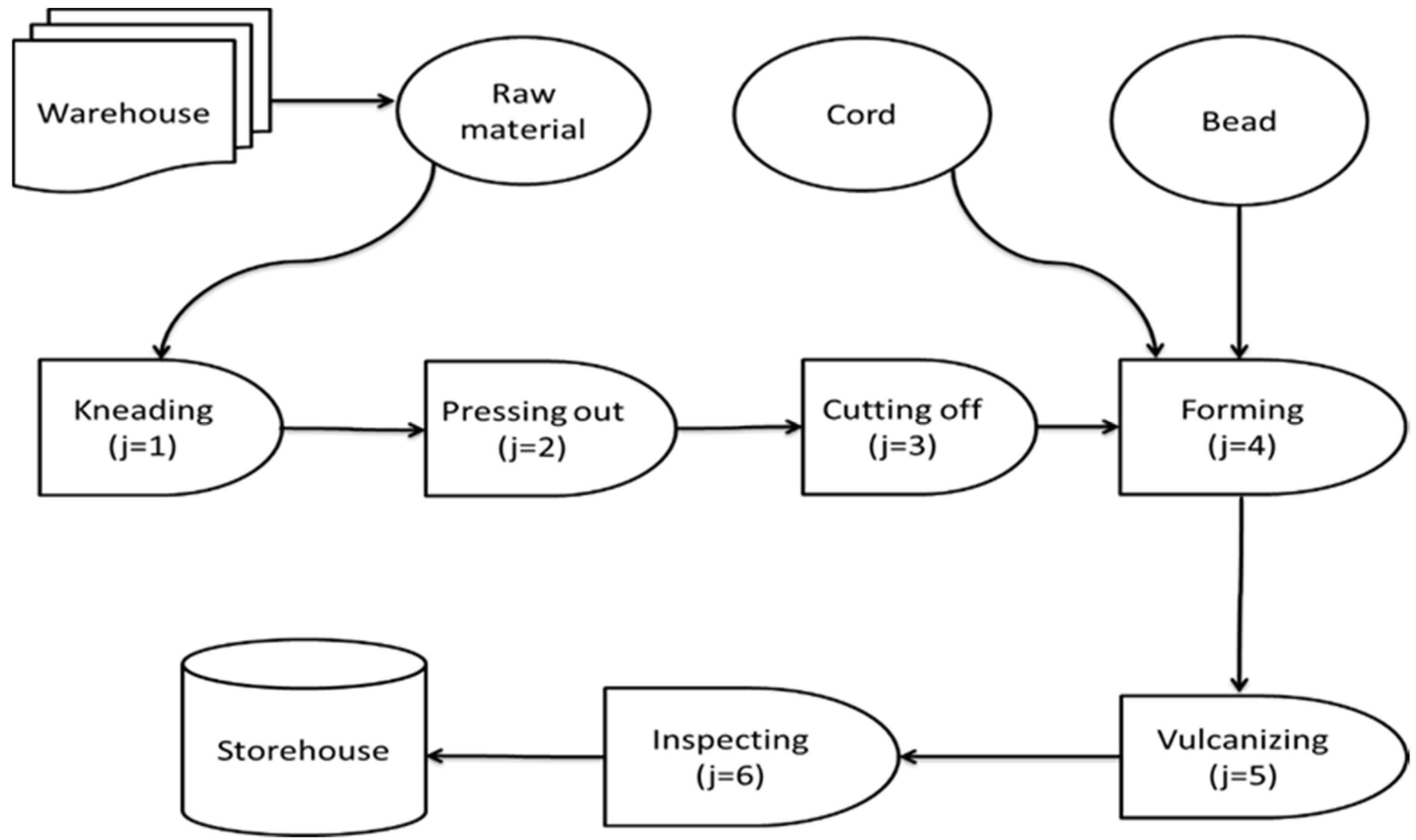
The manufacturing processes of the tire industry are complex and have six main processes: kneading, pressing out, cutting off, forming, vulcanizing, and inspecting (as shown in Figure 1):
- Kneading (j = 1): The first process mixes all the rubber materials and soot, and transports them to the kneader for kneading to change the strength of the rubber.
- Pressing out (j = 2): The second process uses glue and friction to generate heat, allowing the rubber to mature.
- Cutting off (j = 3): The third process mainly uses a cutting machine to cut off various tire sizes.
- Forming (j = 4): The fourth process is to perform the molding assembly work to assembly all the materials, strips, and steel rings to complete the tire prototype.
- Vulcanizing (j = 5): The fifth process is to perform the vulcanization process. The main purpose of tire vulcanization is to rearrange the molecules of the rubber, meaning to heat and mold the tires through steam. The tires that complete this process will become the finished tires.
- Inspecting (j = 6): Finally, the finished tires are inspected and the tires are moved to the warehouse for shipment.
3.2. The Model Formulation
From the aforementioned ABC model and the main tire manufacturing process, the corresponding costs are included in the mathematical model. First, this article assumes that the unit product prices are constant within a certain relevant range. Second, the green activity for each production process, as well as its activity driver and related resources, are determined and selected. Third, five materials (natural rubber, soot, synthetic rubber, cord, and bead) used in the production process are the direct material inputs, while other insignificant materials are not included in this study. Fourth, direct labor resources can be increased by additional overtime work with higher wage rates. Fifth, assume that carbon emission costs are considered as variable costs, which depend on carbon emissions quantity and different tax rates. Organic compounds are chemicals that contain carbon and are found in all living things. In addition to carbon, carbon contains other elements, such as hydrogen, oxygen, fluorine, chlorine, bromine, sulfur or nitrogen. Assume that the relationship between carbon tax and carbon emission quantity has been set up by using the concept of carbon equivalency. Sixth, this research is limited by the difficulty of obtaining relevant information, thus, we only consider the direct materials, direct labor, disposal costs, and carbon emissions costs, and assume that all other costs are fixed costs. The data used in this study are in metric tons and U.S. dollars, as shown in Table 1.
Since the traditional cost system analyzes the cost, most of it is based on direct raw materials, direct labor, and indirect manufacturing costs. The ABC cost system allocates resources to the activity or activity center according to the resource driver, and the activity cost is distributed to the product according to the activity drivers. Through the implementation of the analysis method, the cost of each activity can be correctly calculated. In addition, the TOC theory proposes some standardization methods for defining and eliminating constraints in manufacturing activities. The enterprise is a system, the goal is to obtain more profits, and all the factors that hinder the achievement of the overall goal are constraints, in order to measure the realization. The performance and effectiveness of the target, TOC breaks the traditional concept of accounting costs. In summary, this paper inspires the innovative thinking, applies ABC cost system, TOC theory combined with mathematical planning to establish the model, the objective function and its constraints are described in the sections that follow.
3.2.1. Objective Function
This study establishes the mathematical planning model of the tire industry through the ABC cost system and the TOC theory. Since it is difficult to obtain real cost and expense data, it can be assumed that the factors hindering the target are constraints. Therefore, the following is a discussion of the objective function of the ABC green production model. The objective of the model is to determine the optimal product mix to achieve maximal profit under the constraints of various resources and carbon emissions. The following is the objective of the model:
where Bi is the production quantity of product i; Ci is the unit sales price of product i; Dk is the unit cost of material k; Eik is the requirements of material k for producing a unit of product i; TLC0 is total direct labor costs at LS0; TLC1 is total direct labor costs at LS1; TLC2 is total direct labor costs at LS2; (e0, e1, e2) is a set of non-negative variables of SOS2 (special ordered set of type 2), where at most two adjacent variables may be non-zero in the order of a given set [57,58]; Gi is the other material handling cost, with the exception of machine depreciation per batch of material handling for product i; is the number of batches for material handling of product i; CTi is the total carbon emission cost in CEi; F is the fixed cost.
The profit function of in the model is shown in Equation (1). Total revenue is of Equation (1) in the first term. Direct material cost is of Equation (1) in the second term, direct labor cost is of Equation (1) in the third term, material handing cost is of Equation (1) in the fourth term, carbon emission cost is of Equation (1) in the fifth term, and the other fixed cost is of Equation (1) in the sixth term. Some other costs are fixed; for example, the depreciations of property, plants, and equipment are fixed, thus, they will have the associated constraints of capacity. While fire insurance charges and fundamental utility fees are also fixed, they will not have the associated constraints of capacity. These fixed costs in total can be expressed as a constant F (USD $22,000 in this example data).
3.2.2. The Associated Constraints
(1) Direct material quantity constraints:
where Fk is the quantity of material k available for use. Equation (2) represents the constraints for direct materials and the direct material cost is of Equation (1) in the second term.
(2) Direct labor hour constraints:
where di is the requirement of direct labor hours for one unit of product i; Bi is the production quantity of product i; LS0 is the normal direct labor hours available; LS1 is the maximal working hours at the first overtime rate plus the normal direct labor hours available; LS2 is the maximal working hours at the first and second overtime rate plus the normal direct labor hours available. Equations (3)–(11) are the constraints associated with direct labor. TDL in Equation (3) is the total direct labor hours. The direct labor cost is of Equation (1) in the third term, and the direct labor cost function is shown in Figure 2. (, e1, e2) is a set of non-negative variables of SOS2 (special ordered set of type 2), where at most two adjacent variables may be non-zero in the order of a given set [57,58]; (m1, m2) is a set of 0–1 variables of SOS1 (special ordered set of type 1), where only one must have one variable that will be non-zero [39,40]. If m1 = 1, then m2 = 0 from Equation (8), e2 = 0 from Equation (6), e0, e1 1 from Equations (4) and (5), and e0 + e1 = 1 from Equation (7). Therefore, total direct labor hours and total labor costs are and , respectively, which means that the company works overtime at the first overtime rate. On the other hand, if m2 = 1, then = 0 from Equation (8), = 0 from Equation (4), , ≤ 1 from Equations (5) and (6), and + = 1 from Equation (7). Thus, the total direct labor hours required is from Equations (3) and the total labor cost is , respectively, which means there will be overtime work at the second overtime rate. When m1 = 1 and = 1, then m2 = e1 = e2 = 0 from Equations (4)–(9), total direct labor hours = , and the total labor cost is .
(3) Machine hour constraints:
where bij is the number of machine hours required to produce one unit of product i in activity j; Bi is the production quantity of product i; and Hj is the number of machine hours i available for activity j. Each process requires a different machine for related activities and Equation (12) is the machine hour constraints.
(4) Material handing constraints:
where Bi is the production quantity of product i; is the number of batches for product i; is the quantity of product i in a batch of material handling activity; is the requirement of machine hours for product i in a batch of material handling activity; (j = 7) is the machine hours available for material handling. The material handling activity is a batch-level activity. Equation (13) is the constraints regarding the relationship between the quantity of product i () and the number of batches for product i; Equation (14) is the resource constraint for the machine hours of material handling activity. In the tire manufacturing process, the relevant materials must be moved from the warehouse to the first process, and then, move the finished tires from the last process to the warehouse. Total material handling cost, with the exception of the depreciation of the material handling machine (it is included in F) is, as follows:
This is the fourth term of Equation (1), where Gi is the other material handling cost, with the exception of machine depreciation per batch of material handling for product i, and is the number of batches for material handling of product i.
(5) Carbon emissions constraints:
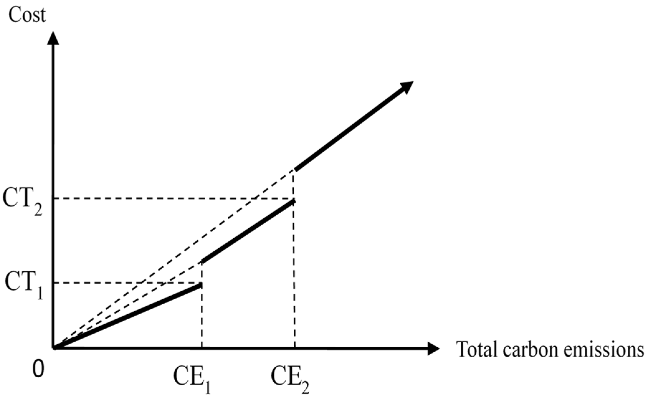
where in the total carbon emission quantity in the tire company; is the carbon emission quantity for one unit of product i; Bi is the production quantity of product i; represents the total carbon emission quantity in the tire company if it falls within the ith range of the total carbon emissions in Figure 3; UCE is the upper limit of the carbon emissions, as distributed to the tire company by the government; is the indicator variable and means that the total carbon emission quantity of the tire company falls within the ith range of the total carbon emissions in Figure 3; and are the highest carbon emission quantities for the first and second carbon emission ranges of the carbon emission cost function in Figure 3, respectively.
Levying taxes could increase GDP. Energy taxes will affect the costs of energy-consumption industries due to rising energy costs [59]. On the other hand, energy taxes can help to reduce the concentration of air pollutants, thereby, improving air quality. In addition, calculating capital and operating expenses is based on a simulation of carbon emissions and economic performance under efficiency taxes, as based on the obtained quality and energy balances; the research results of levying carbon taxes show that all of the assessed environmental impact indicators are performing well [60], the new green manufacturing technology (GMT) can reduce carbon emissions [61], which uses a Life Cycle Assessment (LCA) method to measure emissions costs. LCA is a method for assessing the environment over the entire life cycle of a product or service. Based on previous research, we consider all the environmental impacts of carbon emissions in the tire manufacturing process, and reduce carbon footprint through the development of innovative materials and manufacturing sustainability. Other studies have reduced the carbon footprint resistance of trucking by developing innovative low-rolling, reducing truck tires by at least 20% rolling resistance, roughly equivalent to a 5% reduction in fuel consumption and carbon dioxide emissions. Truck tire wear (10% improvement) and safety performance are further improved [43]. According to the method of Ward and Chapman [62], we quantify carbon emissions in Equation (15). The tax rates for carbon emissions differ, and the total emission cost function is a piecewise discontinuity function (as shown in Figure 3). As carbon emissions increase, taxes will increase [63]. That is: TR1W1, TR2W2, and TR3W3 represent the carbon emission cost when total carbon emission falls within the first, the second, and the third range of Figure 3. Total carbon emission costs are, as follows:
This is the fifth term of Equation (1), i.e., total carbon emissions cost. The related constraints are Equations (15)–(22). In Equations (17)–(22), (, , ) is a SOS2 set of 0–1 variables, and only one and just one will be 1. If = 1, then , = 0 from Equation (22), from Equations (17) and (18), from Equations (19)–(21); that is, the total carbon emission quantity falls within the first range [0, CE1] of Figure 3, and the total carbon emission cost is . Similarly, if = 1, then the total carbon emission quantity falls within the first range (, ] of Figure 3, and the total carbon emission cost is ; if n3 = 1, then the total carbon emission quantity falls within the third range (, ∞) of Figure 3, and the total carbon emission cost is . The cost function of Figure 3 is a carbon emission cost function with full progressive tax rates. In summary, the more the tire company generates carbon emissions, the more it should pay for carbon emission taxes.
3.3. Summary
In summary, the above discussion includes the manufacturing process of the tire industry, the application of ABC cost system and TOC theory in mathematical programming, revenue, various costs, and carbon emissions in the objective function and the associated constraints. In the following sections, scenario analysis will be conducted using the assumed three carbon emission cost models. The results of the analysis will be provided for management decision-making.
4. Illustration
The tire company burns exhaust during the production process, and the emission of carbon seriously affects air pollution. This paper proposes a hypothetical discussion of a green decision model for tire Company A. As an illustration, company A in the tire industry has been established in Taiwan for more than 50 years. There are 11 tire manufacturing companies in the world, with more than 24,000 employees worldwide and paid-in capital exceeding 30 billion yuan. The main products are all kinds of tires and rubber products. Company A is used to illustrate how to apply the green decision-making model proposed in this paper. We assume that Company A’s costs for producing their products include direct material cost, direct labor cost, kneading activity cost, pressing out activity cost, cutting off activity cost, forming activity cost, vulcanizing activity cost, inspecting activity cost, material handing activity cost, and carbon emission cost (tax).
4.1. Model 1: Green Decision Model without Carbon Rights Trading, but Has a Carbon Cap Allocated for Use by the Government
When using Equations (1)–(22), let Company A consider the production of three main products: Passenger Car Radial (PCR) product (i = 1), Truck & Bus Radial (TBR) product (i = 2), and Motorcycle (MC) product (i = 3), and that these products consume the same direct materials. Then, each product’s quantity is shown in thousands, and the costs and input costs are in U.S. dollars. The data for the case are shown in Table 1. Total fixed cost is a constant (USD $22,000 in this example). This study uses the illustrative example data in Table 1 for the three green decision models explored in this paper, including a model without carbon rights trading and two models with two kinds of carbon rights trading costs, in order to analyze the carbon emission costs in the tire industry for managerial decisions.
The green product mix decision model without carbon rights trading for the case data in Table 1 is shown in Table 2. We solved this o-1 mixed integer programming (0–1 MIP) model by using LINGO 16.0 software, and the optimal solution is shown at the bottom area of Table 2.
The total profit Z is USD $53,225,000. It is assumed that the government allocates a carbon emission quantity to Company A, which has been converted to the carbon emission quantity UCE = 4,000,000 metric tons, and the carbon emission cost (tax) is shown in Figure 3. The carbon tax cost function fz(GCE) are, as follows:
The optimal solution in Table 2 indicates that the total carbon emission quantity is 335,000 metric tons and the carbon emission cost is USD $3,350,000, which falls in the first range of carbon emission quantity in Figure 3. If the remaining 3,665,000 metric tons of carbon emission quantity can be sold to other companies that need to purchase additional carbon credits, according to the EU (2008–2012) under the emissions trading scheme, and is sold at USD $30 per metric ton of carbon dioxide, the tire industry could add an additional profit of USD $109,950,000 to increase its existing maximum gross profit to USD $163,175,000 (=$53,225,000 + $109,950,000).
According to the results of this scenario analysis as shown in Table 2, if the tire industry controls the carbon emission cost according to this mathematical programming model and sells the remaining carbon emissions allocated from the government to the companies that need to purchase carbon emissions. In addition to the original income of the products, the company can also get a considerable income to sell the remaining carbon emissions. It can be seen that carbon emissions are indeed a very important indicator variable affecting the tire company’s profit, and the tire industry should carefully control carbon emissions to avoid cost explosion on the premise of maximizing profits.
4.2. Model 2: Green Decision Model with Constant Carbon Right Cost
Model 2 assumes that the company can purchase carbon rights with a constant unit cost (R). The carbon right cost function is equal to the , as shown in Figure 4, if the company has the need to buy carbon right for additional sales.
The company’s carbon emission cost function is equal to the carbon tax cost plus the carbon right purchase cost. The carbon emission cost function f2 (GCE) is as follows:
where is the carbon tax cost function and is carbon right cost function. When the company’s carbon emission quantity does not exceed the carbon emission quota (UCE), the carbon emission cost only includes the carbon tax cost , otherwise, the company needs to buy carbon right, and the company’s carbon emission cost is .
The objective for Model 2 is shown as follows:
The additional associated constraints are, as follows:
where R is the unit cost of carbon right; UCPQ is the maximum quantity of carbon right that the company can purchase. and are indictor variables of 0–1 variables. If , then from Equation (29), from Equations (27) and (28), and UCE from Equations (25) and (26). That is, the company need not purchase the carbon rights, and the total carbon emission cost is ( + + ) from Equation (23). On the other hand, if , then from Equation (29), from Equations (25) and (26), and UCE (UCE + UCPQ) from Equations (27) and (28). That is, the company needs to purchase carbon rights at the quantity, (GCE − UCE), and the total carbon emission cost is [( + + ) + R*(GCE − UCE)]. Other variables and parameters are as previously defined.
Equations (2)–(29) form Model 2, as explored in this paper. In Model 2, it is assumed that the carbon rights can be purchased regarding the required carbon emissions, and according to the EU (2008–2012) under the emissions trading scheme, the constant cost per unit tonne of carbon dioxide is USD $30 (R). Assume also that the maximal quantity of carbon rights that the company can purchase (UCPQ) is 160 tonnes of carbon dioxide. Model 2 with R = USD $30, UCPQ = 160, and the illustrative data in Table 1, is as shown in Table 3. We solve this problem and the optimal solution is shown at the bottom area of Table 3. The optimal solution indicates that the required carbon footprint of Company A exceeds the maximum amount of carbon credits, as allocated by the government.
The results of this scenario analysis are compared with scenario 1 and it is found that scenario 2 assumes that carbon rights are purchased, the maximum profit will be reduced by USD $175,000 (from USD $53,225,000 to USD $53,050,000) and carbon emissions will increase by 1000 metric tons. (by 335,000 metric tons increased to 336,000 metric tons). The results of this scenario analysis also prove that carbon emissions are indeed variables that affect the total profitability. It can also provide the tire industry in the future when purchasing carbon rights, we should carefully consider the company’s overall revenue, and avoid the purchase and use of carbon rights, so that the cost can be optimally controlled, so that the company will continue to operate.
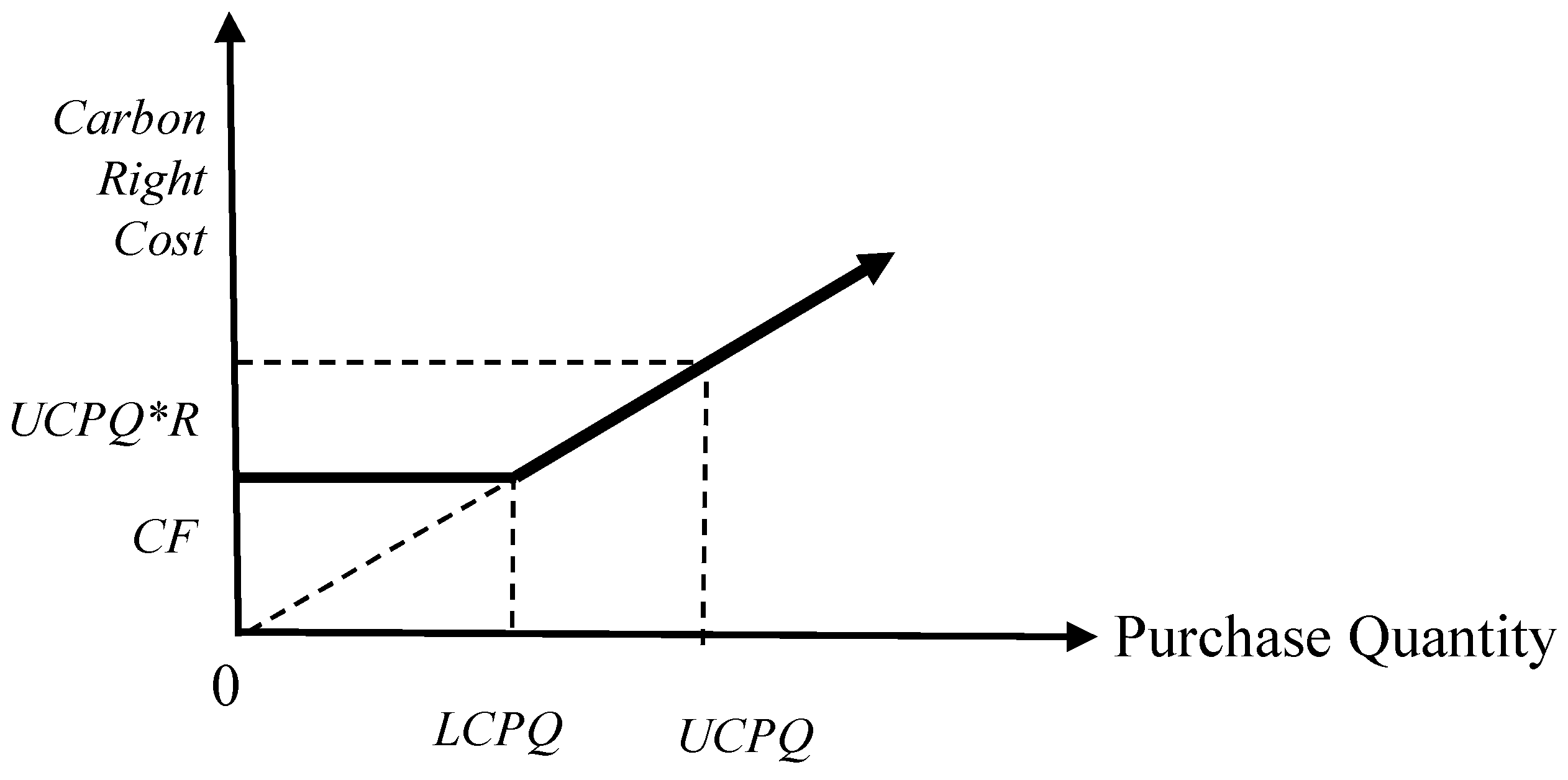
4.3. Model 3: Green Decision Model with a Minimum Purchase Quantity of Carbon Right
Model 3 assumes that the company should purchase the carbon right with a minimum purchase quantity (LCPQ) that has a constant charge (CF) if the company has the need for additional sales, as shown in Figure 5 and the carbon emission cost function f3 (GCE) is as follows:
where, there are three scenarios for the carbon emission cost function: (1) the company’s carbon emission quantity does not exceed the carbon emission quota (UCE), (2) the company needs to buy the carbon right whose quantity does not exceed the LCPQ, (3) the company needs to buy the carbon right whose quantity between LCPQ and UCPQ.
The objective for Model 3 is shown as follows:
The additional associated constraints are, as follows:
where R is the unit cost of carbon right; LCPQ is the minimum purchase quantity; and UCPQ is the maximum quantity of carbon right that the company can purchase. , , and are indictor variables of 0–1 variables. If , then from Equation (38), from Equations (34)–(37), and UCE from Equations (32)–(33). That is, the company need not purchase carbon rights, and the total carbon emission cost is ( + + ) from Equation (30). If , then from Equation (38), from Equations (32)–(33) and (36)–(37), and UCE (UCE + LCPQ) from Equations (34)–(35). That is, the company needs to purchase carbon rights at the minimum purchase quantity, LCPQ, and the total carbon emission cost is [( + + ) + CF]. If , then . from Equation (38), from Equations (32)–(35), and (UCE + UCPQ) from Equations (36)–(37). That is, the company needs to purchase carbon rights exceeding the minimum purchase quantity, LCPQ, and the total carbon emission cost is [( + + ) + CF + R*(GCE − UCE − LCPQ)]. Other variables and parameters are as previously defined.
Equations (2)–(22) and (30)–(38) form Model 3, as studied in this paper. As in Model 2, it is assumed that R = USD $30 and UCPQ = 160. Assume also that the minimum purchase of carbon rights is 60,000 metric tonnes, i.e., LCPQ = 60; then, CF = R*LCPQ = $1800. Model 3, with these data and the illustrative data in Table 1, is shown in Table 4. We solve this problem and the optimal solution is shown at the bottom area of Table 4. The optimal solution indicates that the required carbon footprint of 4,060,000 tonnes for Company A is equal to (UCE + LCPQ). It means that Company A needs to obtain just the minimum purchase quantity of 60,000 metric tonnes of carbon rights in addition to the permissible no need to buy carbon rights emission quantity (UCE), as allocated by the government. As a result, the optimal green portfolio decision and the maximum total profit obtained is USD $53,050,000.
The result of this scenario is the same as scenario 2. It means that if the tire industry needs to purchase carbon rights, it will affect the total profit. From the results of the scenario analysis, it is further proved that the purchase of carbon rights will affect the total profit of the tire industry. If carbon tax is levied, in the cost control, special attention should be paid to the quantity of carbon emissions for which there is no need to buy carbon rights to avoid cost explosions.
4.4. Sensitivity Analysis
One of important things for enterprises is the maximization of total profits, thus, this article focuses on high-carbon emission and high-polluting tire industries. With the rise of environmental awareness, corporate carbon emissions policies have been implemented in the branches of other countries. Insufficient carbon emissions due to the allocation of the country will require the additional acquisition of carbon rights, which will result in an additional burden on costly carbon emissions. To further understand the impact of the three key variables of the carbon emissions trading model on total profits in this study, three types of model carbon tax rates were increased or decreased by 5% to 30% for a total of 12 cases for sensitivity analysis (Table 5, Table 6 and Table 7). The test results are, as follows:
- (1)
- Model 1: The original total profit of the company is USD $53,225, and the carbon tax rate is increased by 5%, 10%, 15%, 20%, 25%, and 30%, respectively. The total profit found was reduced by 0.31% (USD $53,057,500), 0.62% (USD $52,890,000), 0.94% (USD $52,772.50), 1.25% (USD $52,555,000), 1.57% (USD) $52,387.50), and 1.88% (USD $52,200), respectively; at the relative decreases of 5%, 10%, 15%, 20%, and 25%, then the total profit was found to increase by 0.31% (USD $53,392.50), 0.62% (USD $53,560), and 0.94% (USD $53,727.50), 1.25% (USD $53,895), 1.57% (USD $54,062.50), and 1.88% (USD $54,230), respectively. Therefore, as the carbon tax rate decreases, the total profit of the enterprise will increase. Conversely, increasing the carbon tax rate will lead to a decrease in total corporate profits.
- (2)
- Model 2: The original total profit of the company was USD $53,225, the carbon tax rate was increased by 5%, 10%, 15%, 20%, and 25%, respectively, and the total profit was found to decrease by 0.31% (USD $52,882), 0.63% (USD $52,714), 0.95% (USD $52,546), 1.26% (USD $52,378), 1.58% (USD $52,210), and 1.9% (USD $52,042), respectively; at the relative decrease of 5%, 10%, 15%, 20%, 25%, and 30%, it is found that the total profit increased by 0.31% (USD $53,218), 0.63% (USD $53,386), 0.95% (USD $53,554), 1.26% (USD $53,722), 1.58% (USD $53,890), and 1.9% (USD $54,058), respectively. Therefore, as the carbon tax rate decreases, the total profit of the company will increase. Conversely, increasing the carbon tax rate will lead to a decrease in total corporate profits.
- (3)
- Model 3: The original total profit of the company is USD $53,050, and the carbon tax rate is increased by 5%, 10%, 15%, 20%, 25%, and 30% respectively. The total profit found was reduced by 0.31% (USD $52,882), 0.63% (USD $52,714), 0.95% (USD $52,546), 1.26% (USD $52,378), 1.58% (USD $52,210), and 1.9% (USD $52,042), respectively. At the relative decrease of 5%, 10%, 15%, 20%, 25%, and 30%, it is found that the total profit increased by 0.31% (USD $53,218), 0.63% (USD $53,386), 0.95% (USD $53,554), 1.26% (USD $53,722), 1.58% (USD $53,890), and 1.9% (USD $54,058), respectively. Therefore, as the carbon tax rate decreases, the total profit of the company will increase. Conversely, increasing the carbon tax rate will lead to a decrease in total corporate profits.
In summary, three different scenario models with carbon taxes and carbon right are analyzed in this study by sensitivity analysis, and the results show that the increase or decrease of the carbon tax rate is one of the major factors affecting the total profit of the tire industry. However, under the current international focus on greenhouse gas emission reduction and environmental protection, how to reduce carbon emissions has become an important issue. The implementation of the national carbon emission system and carbon rights trading system is the most important issue for international environmental protection today. Therefore, the tire industry should understand the response to the implementation of the carbon tax, as well as the additional costs of carbon emission exchanges, in order to avoid affecting the company’s biggest profit decline.
5. Conclusions
The tire industry is a high-carbon and high-pollution industry. As global warming, climate change, and global emissions of greenhouse gases have become international environmental issues of concern, in recent years, some countries have encountered air pollution and environmental problems, and have begun to adopt the carbon price mechanism to implement carbon taxes. Therefore, the carbon tax and the carbon trading mechanism are the main strategies used by various governments around the world to respond to global warming and promote a green economy. Based on this concept, this paper applied a mathematical programming model and put forward three green optimal carbon price models for analysis. In Model 1, the results show that the tire company can sell the remaining 3,664,000 metric tonnes to other companies in need, and thus, earn more money. In addition, based on the assumptions of the two carbon rights purchase cost models of Model 2 and Model 3, analysis shows that the tire companies do not need to purchase additional carbon rights; however, compared with Model 1, if there is a carbon rights transaction, the total profit will decrease. Therefore, in order to reduce the impact of carbon tax and carbon trading on the profits of tire companies, tire companies could reduce carbon emissions as much as possible, and they can significantly reduce costs to create higher profits.
Based on the mathematical programming model, this article developed three different scenario models with carbon tax and carbon right for tire companies and conducted sensitivity analysis. The analysis results can provide references for tire industry management’s decision-making. In addition, according to the analysis results, we know that the operating costs will increase if a company wants to purchase additional carbon rights, which may led to a substantial reduction in profits. Therefore, management should pay more attention to the quantity of carbon rights purchased. In addition, the mathematical programming model with carbon tax and carbon rights trading, as developed in this paper, can be extended to other relevant industries, such as construction, aviation, paper, steel, and other high pollution industries with high carbon emissions. In addition, this paper can be extended to the development of a green tax system through the design of a long-term and short-term mixed tax policy [64] to reflect the correct price of carbon tax and to reduce carbon emissions and air pollution. It is also possible to consider the policy of carbon emission and carbon pricing from the perspective of economics. Besides, this research can also be extended to consider the carbon emission permit allocation factors or the game-theoretic problem involving more than one company in a cap-and-trade system [65].
Funding
This research was funded by the Ministry of Science and Technology of Taiwan under Grant No. MOST106-2410-H-008-020-MY3.
Acknowledgments
The author is extremely grateful to the energies journal editorial team and reviewers who provided valuable comments for improving the quality of this article. The author also would like to thank the National Science Council of Taiwan for financially supporting this research under Grant No. MOST106-2410-H-008-020-MY3.
Conflicts of Interest
The author declares no conflict of interest.
References
- Baranzini, A.; Carattini, S. Taxation of Emissions of Greenhouse Gases. In Global Environmental Change; Freedman, B., Ed.; Springer: Dordrecht, The Netherlands, 2014; pp. 543–560. [Google Scholar]
- Energy Leaders Accelerate Climate Action Global Climate Action at COP22, UNFCCC. 2016. Available online: http://newsroom.unfccc.int/climate-action/energy-leaders-accelerate-climate- action/ (accessed on 3 July 2018).
- Sarkar, B.; Ahmed, W.; Kim, N. Joint effects of variable carbon emission cost and multi-delay-in-payments under single-setup-multiple-delivery policy in a global sustainable supply chain. J. Clean. Prod. 2018, 185, 421–445. [Google Scholar] [CrossRef]
- Schaltegger, S.; Synnestvedt, T. The link between ‘green’ and economic success: Environmental management as the crucial trigger between environmental and economic performance. J. Environ. Manag. 2002, 65, 339–346. [Google Scholar]
- Baranzini, A.; Goldemberg, J.; Speck, S. A Future for Carbon Taxes. Ecol. Econ. 2000, 32, 395–412. [Google Scholar] [CrossRef]
- Metcalf, G.E. Designing a Carbon Tax to Reduce U.S. Greenhouse Gas Emissions. Rev. Environ. Econ. Policy 2009, 3, 63–83. [Google Scholar] [CrossRef]
- Fang, G.; Tian, L.; Liu, M.; Fu, M.; Sun, M. How to optimize the development of carbon trading in China—Enlightenment from evolution rules of the EU carbon price. Appl. Energy 2018, 211, 1039–1049. [Google Scholar] [CrossRef]
- Martin, R.; Muûls, M.; De Preux, L.B.; Wagner, U.J. Industry Compensation under Relocation Risk: A Firm-Level Analysis of the EU Emissions Trading Scheme. Am. Econ. Rev. 2014, 104, 2482–2508. [Google Scholar] [CrossRef] [Green Version]
- Goulder, L.H.; Parry, I.W. Instrument Choice in Environmental Policy. Rev. Environ. Econ. Policy 2008, 2, 152–174. [Google Scholar] [CrossRef] [Green Version]
- Fan, J.H.; Todorova, N. Dynamics of China’s carbon prices in the pilot trading phase. Appl. Energy 2017, 208, 1452–1467. [Google Scholar] [CrossRef]
- Lin, B.; Jia, Z. The impact of Emission Trading Scheme (ETS) and the choice of coverage industry in ETS: A case study in China. Appl. Energy 2017, 205, 1512–1527. [Google Scholar] [CrossRef]
- Sathre, R.; Gustavsson, L. Effects of energy and carbon taxes on building material competitiveness. Energy Build. 2007, 39, 488–494. [Google Scholar] [CrossRef]
- Basanta, K.; Pradhan, J.G.; Yao, Y.F.; Liang, Q.M. Carbon pricing and terms of trade effects for China and India: A general equilibrium analysis. Econ. Model. 2017, 63, 60–74. [Google Scholar]
- Maryniak, P.; Trück, S.; Weron, R. Carbon pricing and electricity markets—The case of the Australian Clean Energy Bill. Energy Econ. 2018. [Google Scholar] [CrossRef]
- Kee, R.; Schmidt, C. A comparative analysis of utilizing activity-based costing and the theory of constraints for making product-mix decisions. Int. J. Prod. Econ. 2000, 63, 1–17. [Google Scholar] [CrossRef]
- Massood, Y.Z. Product-mix decisions under activity-based costing with resource constraints and non-proportional activity costs. J. Appl. Bus. Res. 1998, 14, 39–46. [Google Scholar]
- Lockhart, J.; Taylor, A. Environmental Considerations in Product Mix Decisions Using ABC and TOC. Manag. Account. Q. 2007, 9, 13–31. [Google Scholar]
- Onwubolu, G.C.; Mutingi, M. Optimizing the multiple constrained resources product mix problem using genetic algorithms. Int. J. Prod. Res. 2001, 39, 1897–1910. [Google Scholar] [CrossRef]
- Fernández, Y.F.; Fernández López, M.A.; Blanco, B.O. Innovation for sustainability: The impact of R&D spending on CO2 emissions. J. Clean. Prod. 2018, 172, 3459–3467. [Google Scholar]
- Hoinka, K.; Ziębik, A. Mathematical model for the choice of an energy management structure of complex buildings. Energy 2010, 35, 1146–1156. [Google Scholar] [CrossRef]
- Chen, X.; Chan, C.K.; Lee, Y.C.E. Responsible production policies with substitution and carbon emissions trading. J. Clean. Prod. 2016, 134, 642–651. [Google Scholar] [CrossRef]
- Chen, X.; Luo, Z.; Wang, X. Impact of efficiency, investment, and competition on low carbon manufacturing. J. Clean. Prod. 2017, 143, 388–400. [Google Scholar] [CrossRef]
- Du, Z.; Lin, B. Analysis of carbon emissions reduction of China’s metallurgical industry. J. Clean. Prod. 2018, 176, 1177–1184. [Google Scholar] [CrossRef]
- Baranzini, A.; Van den Bergh, J.C.; Carattini, S.; Howarth, R.B.; Padilla, E.; Roca, J. Carbon Pricing in Climate Policy: Seven Reasons, Complementary Instruments, and Political Economy Considerations. Wiley Interdiscip. Rev. Clim. Chang. 2017, 8, e462. [Google Scholar] [CrossRef]
- Aldy, J.E.; Stavins, R.N. The Promise and Problems of Pricing Carbon: Theory and Experience. J. Environ. Dev. 2012, 21, 152–180. [Google Scholar] [CrossRef]
- CDP. Putting a Price on Carbon: Integrating Climate Risk into Business Planning; CDP Report: Carbon Disclosure Project; CDP: London, UK, 2017; Available online: https://b8f65cb373b1b7b15feb-c70d8ead6ced550b4d987d7c03fcdd1d.ssl.cf3.rackcdn.com/cms/reports/documents/000/002/738/original/Putting-a-price-on-carbon-CDP-Report-2017.pdf?1507739326 (accessed on 3 July 2018).
- Zheng, G.; Jing, Y.; Huang, H.; Zhang, X.; Gao, Y. Application of life cycle assessment (LCA) and extenics theory for building energy conservation assessment. Energy 2009, 34, 1870–1879. [Google Scholar] [CrossRef]
- Fang, Y.P.; Zeng, Y. Balancing energy and environment: The effect and perspective of management instruments in China. Energy 2007, 32, 2247–2261. [Google Scholar] [CrossRef]
- Lee, C.F.; Lin, S.J.; Lewis, C. Analysis of the impacts of combining carbon taxation and emission trading on different industry sectors. Energy Policy 2008, 36, 722–729. [Google Scholar] [CrossRef]
- Martin, R.; Muuls, M.; Wagner, U.J. The Impact of the European Union Emissions Trading Scheme on Regulated Firms: What Is the Evidence after Ten Years? Rev. Environ. Econ. Policy 2016, 10, 129–148. [Google Scholar] [CrossRef]
- Oestreich, A.M.; Tsiakas, I. Carbon Emissions and Stock Returns: Evidence from the EU Emissions Trading Scheme. J. Bank. Financ. 2015, 58, 294–308. [Google Scholar] [CrossRef]
- Herber, B.P.; Raga, J.T. An international carbon tax to combat global warming: An economic and political analysis of the European Union proposal. Am. J. Econ. Sociol. 1995, 54, 257–267. [Google Scholar] [CrossRef]
- Nadel, S. Learning from 19 Carbon Taxes: What Does the Evidence Show? In Proceedings of the 2016 ACEEE Summer Study on Energy Efficiency in Buildings, Pacific Grove, CA, USA, 21–26 August 2016; pp. 9-1–9-7. Available online: https://aceee.org/files/proceedings/2016/data/papers/9_49.pdf (accessed on 3 July 2018).
- Xu, J.; Qiu, R.; Lv, C. Carbon emission allowance allocation with cap and trade mechanism in air passenger transport. J. Clean. Prod. 2016, 131, 308–320. [Google Scholar] [CrossRef]
- Johansson, B. Climate policy instruments and industry—Effects and potential responses in the Swedish context. Energy Policy 2006, 34, 2344–2360. [Google Scholar] [CrossRef]
- Liu, Y.; Chen, S.; Chen, B.; Yang, W. Analysis of CO2 emissions embodied in China’s bilateral trade: A non-competitive import input–output approach. J. Clean. Prod. 2017, 163, S410–S419. [Google Scholar] [CrossRef]
- Wang, B.; Liu, B.; Niu, H.; Liu, J.; Yao, S. Impact of energy taxation on economy, environmental and public health quality. J. Environ. Manag. 2017, 206, 85–92. [Google Scholar] [CrossRef] [PubMed]
- Cheng, B.; Dai, H.; Wang, P.; Zhao, D.; Masui, T. Impacts of carbon trading scheme on air pollutant emissions in Guangdong Province of China. Energy Sustain. Dev. 2015, 27, 174–185. [Google Scholar] [CrossRef]
- Ivan, D.R.; Tulloch, D.J. Carbon pricing and system linking: Lessons from the New Zealand Emissions Trading Scheme. Energy Econ. 2018, 73, 66–79. [Google Scholar]
- Roy, C.; Labrecque, B.; Caumia, B.D. Recycling of scrap tires to oil and carbon black by vacuum pyrolysis. Resour. Conserv. Recycl. 1990, 4, 203–213. [Google Scholar] [CrossRef]
- Cooper, R.; Kaplan, R.S. The Design of Cost Management Systems, 2nd ed.; Prentice-Hall: Upper Saddle River, NJ, USA, 1999. [Google Scholar]
- Puurunen, K.; Vasara, P. Opportunities for utillising nanotechnology in reaching near-zero emissions in the paper industry. J. Clean. Prod. 2007, 15, 1287–1294. [Google Scholar] [CrossRef]
- Duez, B. Towards a Substantially Lower Fuel Consumption Freight Transport by the Development of an Innovative Low Rolling Resistance Truck Tyre Concept. Trans. Res. Proced. 2016, 14, 1051–1060. [Google Scholar] [CrossRef]
- Wikipedia, Carbon Tax. Available online: https://en.wikipedia.org/wiki/Carbon_tax (accessed on 3 July 2018).
- Lin, B.; Li, X. The effect of carbon tax on per capita CO2 emission. Energy Policy 2011, 39, 5137–5146. [Google Scholar] [CrossRef]
- Conegrey, T.; Gerald, J.D.F.; Valeri, L.M.; Tol, R.S.J. The impact of a carbon tax on economic growth and carbon dioxide emissions in Ireland. J. Environ. Plan. Manag. 2013, 56, 934–952. [Google Scholar] [CrossRef]
- Kee, R. The sufficiency of product and variable costs for production-related decisions when economies of scope are present. Int. J. Prod. Econ. 2008, 114, 682–696. [Google Scholar] [CrossRef]
- Dekker, R.; Bloembof, J.; Mallidis, I. Operations resarch for greenlogistics—An overview of aspects, issues, contributions and challenges. Eur. J. Oper. Res. 2012, 219, 671–679. [Google Scholar] [CrossRef]
- Tsai, W.H.; Lin, W.R.; Fan, Y.W.; Lee, P.L.; Lin, S.J.; Hsu, J.L. Applying A Mathematical Programming Approach for A Green Product Mix Decision. Int. J. Prod. Res. 2012, 50, 1171–1184. [Google Scholar] [CrossRef]
- Qian, L.; David, B.A. Parametric cost estimation based on activity-based costing: A case study for design and development of rotational parts. Int. J. Prod. Econ. 2008, 113, 805–818. [Google Scholar] [CrossRef]
- Tsai, W.H.; Lin, S.J.; Liu, J.Y.; Lin, W.R.; Lee, K.C. Incorporating life cycle assessments into building project decision-making: An energy consumption and CO2 emission perspective. Energy 2011, 36, 3022–3029. [Google Scholar] [CrossRef]
- Tsai, W.H.; Lin, S.J.; Lee, Y.F.; Chang, Y.C.; Hsu, J.L. Construction method selection for green building projects to improve environmental sustainability by using an MCDM approach. J. Environ. Plan. Manag. 2013, 56, 1487–1510. [Google Scholar] [CrossRef]
- Tsai, W.H.; Yang, C.H.; Huang, C.T.; Wu, Y.Y. The Impact of the Carbon Tax Policy on Green Building Strategy. J. Environ. Plan. Manag. 2017, 60, 1412–1438. [Google Scholar] [CrossRef]
- Plenert, G. Optimizing theory of constraints when multiple constrained resources exist. Eur. J. Oper. Res. 1993, 70, 126–133. [Google Scholar] [CrossRef]
- Tsai, W.H.; Lai, C.W.; Tseng, L.J.; Chou, W.C. Embedding Management Discretionary Power into An ABC Model for A Joint Products Mix Decision. Int. J. Prod. Econ. 2008, 115, 210–220. [Google Scholar] [CrossRef]
- Tsai, W.H.; Kuo, L.; Lin, T.W.; Kuo, Y.C.; Shen, Y.S. Price elasticity of demand and capacity expansion eatufres in an enhanced ABC product-mix Decision Model. Int. J. Prod. Res. 2010, 48, 6387–6416. [Google Scholar] [CrossRef]
- Beale, E.M.L.; Tomlin, J.A. Special facilities in a general mathematical programming system for non-convex problems using ordered sets of variables. Oper. Res. 1970, 69, 447–454. [Google Scholar]
- Williams, H.P. Model Building in Mathematical Programming, 2nd ed.; Wiley: New York, NY, USA, 1985; pp. 173–177. [Google Scholar]
- Wang, Y.; Chen, W.; Liu, B. Manufacturing/remanufacturing decisions for a capital-constrained manufacturer considering carbon emission cap and trade. J. Clean. Prod. 2017, 140, 1118–1128. [Google Scholar] [CrossRef]
- Igor, L.W.; George, V.B.; Jose, L.D.M.; Ofelia, D.Q.F.A. Carbon dioxide utilization in a microalga-based biorefinery: Efficiency of carbon removal and economic performance under carbon taxation. J. Environ. Manag. 2017, 203, 988–998. [Google Scholar]
- Tsai, W.H.; Chen, H.C.; Liu, J.Y.; Chen, S.P.; Shen, Y.S. Using activity-based costing to evaluate capital investments for green manufacturing technologies. Int. J. Prod. Res. 2011, 49, 7275–7292. [Google Scholar] [CrossRef]
- Ward, S.C.; Chapman, C.B. Risk-management perspective on the project lifecycle. Int. J. Proj. Manag. 1995, 13, 145–149. [Google Scholar] [CrossRef]
- Tsai, W.H.; Shen, Y.S.; Lee, P.L.; Chen, H.C.; Kuo, L.; Huang, C.C. Integrating information about the cost of carbon through activity-based costing. J. Clean. Prod. 2012, 36, 102–111. [Google Scholar] [CrossRef]
- Zetterberg, L.; Wråke, M.; Sterner, T.; Fischer, C.; Burtraw, D. Short-Run Allocation of Emissions Allowances and Long-Term Goals for Climate Policy. Ambio 2012, 41, 23–32. [Google Scholar] [CrossRef] [PubMed] [Green Version]
- Du, S.; Ma, F.; Fu, Z.; Zhu, L.; Zhang, J. Game-theoretic analysis for an emission-dependent supply chain in a ‘cap-and-trade’ system. Ann. Oper. Res. 2015, 228, 135–149. [Google Scholar] [CrossRef]
Figure 1.
Tire manufacturing flow chart.

Figure 2.
Direct labor cost.
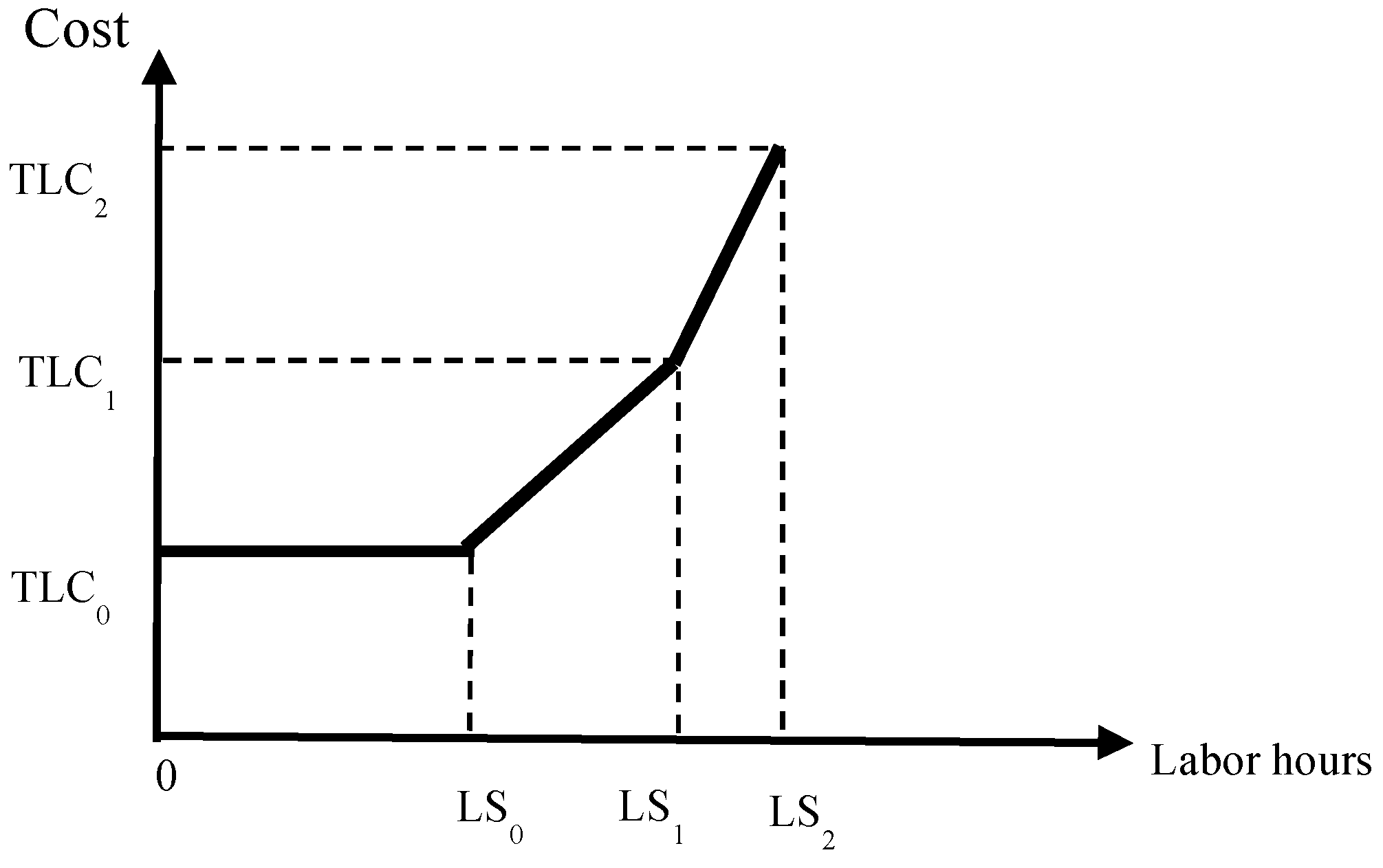
Figure 3.
Carbon emission costs (taxes).

Figure 4.
Carbon right cost.
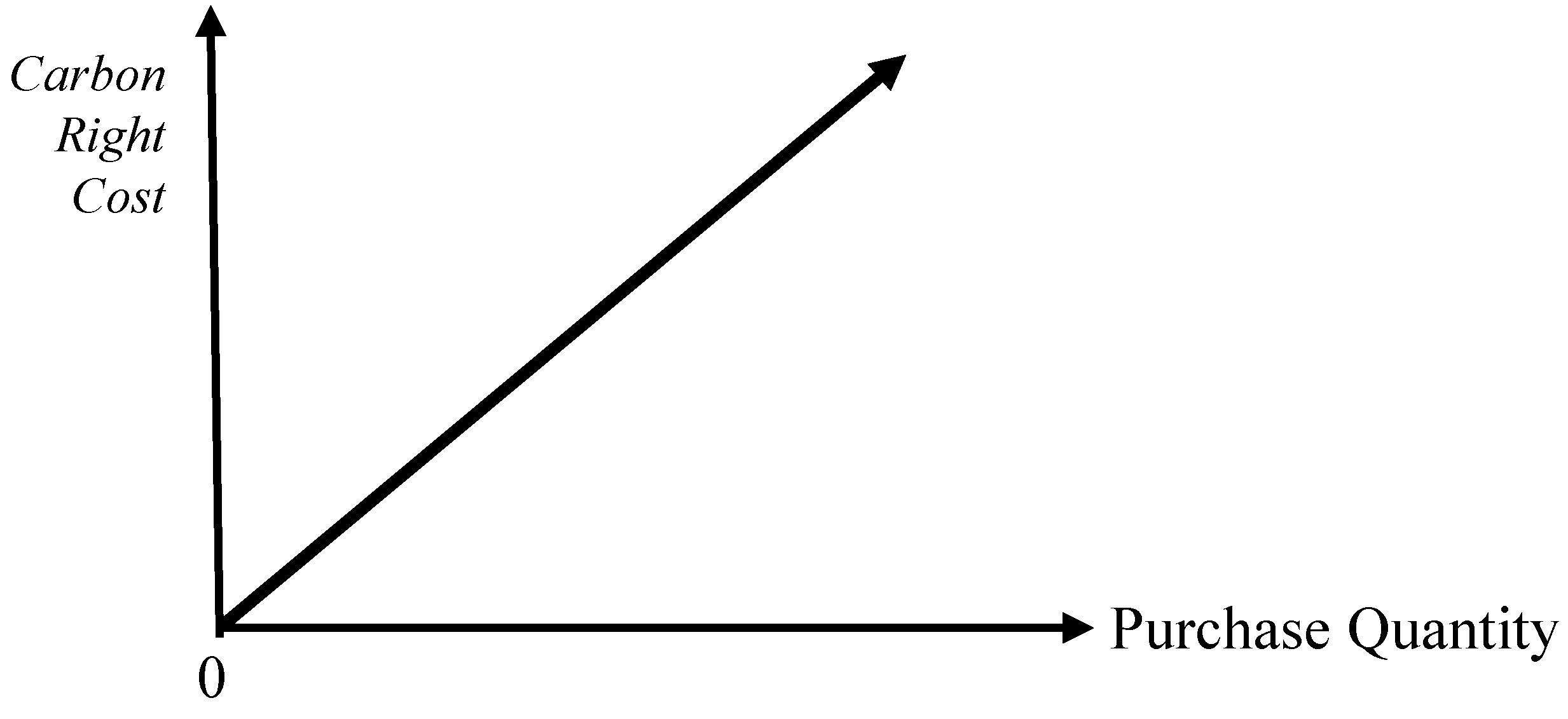
Figure 5.
Carbon right cost.


Table 1.
Data for illustrative example (Company A).
| Product | PCR (i = 1) | TBR (i = 2) | MC (i = 3) | Available Capacity (thousand) | ||||
|---|---|---|---|---|---|---|---|---|
| Maximum demand: (thousand) | j | Bi | 1000 | 100 | 1500 | |||
| Selling price: (USD) | Ci | 310 | 1010 | 160 | ||||
| Direct material: | k = 1 | 21 | 4 | 6 | 2 | F1 = 10,600 | ||
| (USD/ton) | k = 2 | 11 | 2 | 10 | 1 | F2 = 8100 | ||
| k = 3 | 6 | 5 | 15 | 2 | F3 = 8700 | |||
| k = 4 | 38 | 2 | 6 | 1 | F4 = 7100 | |||
| k = 5 | 22 | 2 | 15 | 1 | F5 = 7900 | |||
| Machine hour constraint: | ||||||||
| Kneading | Machine hours | 1 | 5 | 10 | 1 | H1 = 13,300 | ||
| Pressing out | Machine hours | 2 | 2 | 4 | 1 | H2 = 22,100 | ||
| Cutting off | Machine hours | 3 | 2 | 3 | 1 | H3 = 22,100 | ||
| Forming | Machine hours | 4 | 3 | 5 | 1 | H4 = 26,500 | ||
| Vulcanizing | Machine hours | 5 | 2 | 3 | 1 | H5 = 13,300 | ||
| Inspecting | Machine hours | 6 | 3 | 6 | 1 | H6 = 6700 | ||
| Material handling constraint: | ||||||||
| Machine hours (h) Cost (USD) | G1 = 50 G2 = 150 G3 = 10 | 7 | 2 | 3 | 1 | H7 = 1860 | ||
| 5 | 10 | 1 | ||||||
| Direct labor constraint: | ||||||||
| Cost: Labor hours (h) | TLC0 = 7040 | TLC1 = 11,000 | TLC2 = 15,840 | 1 | 1.5 | 0.5 | ||
| LS0 = 1760 | LS1 = 2200 | LS2 = 2640 | ||||||
| Wage rate (USD/h) | r0 = 4 | r1 = 9 | r2 = 11 | |||||
| Carbon emission constraint: | ||||||||
| Cost (USD) Emission quantities | CT1 = 20,400 CE1 = 2040 | CT2 = 46,800 CE2 = 2340 | UCE = 4000 | 0.2 | 0.1 | 0.1 | ||
| Tax rate (USD/ton) | TR1 = 10 | TR2 = 20 | TR3 = 30 | |||||
| Total fixed cost: (USD) | 22,000 | |||||||
[Note] Data in Table 1 are used for Model 1, Model 2, and Model 3.
Table 2.
The model and its optimal solutions with the illustrative data for Model 1.
| Max Z = (310*B1 + 1010*B2 + 160*B3) − (21*4 + 11*2 + 6*5 + 38*2 + 22*2)*B1 − (21*6 + 11*10 + 6*15 + 38*6 + 22*15)*B2-(21*2 + 11*1 + 6*2 + 38*1 + 22*1)*B3 − 7040 − (11,000 − 7040)*e1 − (15,840 − 7040)*e2 − 50*β1 − 150*β2 − 10*β3 − 10*W1 − 20*W2 − 30*W3 − F | |||
| Subject to direct material;4*B1 + 6* B2 + 2* B3 ≤ 10,600; 2*B1 + 10*B2 + 1*B3 ≤ 8100; 5*B1 + 15*B2 + 2*B3 ≤ 8700; 2*B1 + 6*B2 + 1*B3 ≤ 7100; 2*B1 + 15*B2 + 1*B3 ≤ 7900; | Subject to machine hours;5*B1 + 10*B2 + 1*B3 ≤ 13,300; 2*B1 + 4*B2 + 1*B3 ≤ 22,100; 2*B1 + 3*B2 + 1*B3 ≤ 22,100; 3*B1 + 5*B2 + 1*B3 ≤ 26,500; 2*B1 + 3*B2 + 1*B3 ≤ 13,300; 3*B1 + 6*B2 + 1*B3 ≤ 6700; | ||
| Subject to direct labor; 1*B1 + 1.5*B2 + 0.5*B3 − 1760-440*e1 − 880*e2 ≤ 0; e0 − m1 ≤ 0; e1 − m1 – m2 ≤ 0; e2 − m2 ≤ 0; e0 + e1 + e2 = 1; m1 + m2 = 1; 0 ≤ e0 ≤ 1; 0 ≤ e1 ≤ 1; 0 ≤ e2 ≤ 1; m1, m2 = 0,1; | Subject to Material handing; B1 − 5* = 0; B2 − 10* = 0; B3 − 1* = 0; 2* + 3* + 1* ≤ 1860; | ||
| Subject to carbon emission; GCE = , GCE = W1 + W2 + W3; W1 + W2 + W3 ≤ 4000; 0 ≤ W1; W1 ≤ 2040; 2040* < W2; W2 ≤ 2340*; W3 > 2340*; n1 + n2 + n3 = 1. | |||
| The optimal solutions for the example data | |||
| B1 = 895,000 | B2 = 85,000 | B3 = 1,475,000 | F = 22,000,000 |
| e0 = 1 | e1= 0 | e2 = 0 | Z = 53,225,000 |
| β1 = 181,000 | β2 = 8000 | β3 = 1,475,000 | GCE = 335,000 |
| = 1 | = 0 | = 0 | |
| W1 = 335,000 | W2 = 0 | W3 = 0 | |
| = 1 | = 0 | ||
Table 3.
The model and its optimal solutions with the illustrative data for Model 2.
| Max Z = (310*B1 + 1010*B2 + 160*B3) − (21*4 + 11*2 + 6*5 + 38*2 + 22*2)*B1 − (21*6 + 11*10 + 6*15 + 38*6 + 22*15)*B2 − (21*2 + 11*1 + 6*2 + 38*1 + 22*1)*B3 − 7040 − (11,000 − 7040) *e1 − (15,840 − 7040) *e2 − 50* − 150* − 10* − {(10* − 20* − 30*)*θ1 + [(10* − 20* − 30*) + 30*(GCE − 4000)]*θ2} − F | |||
| Subject to direct material; 4*B1 + 6* B2 + 2* B3 ≤ 10,600; 2*B1 + 10*B2 + 1*B3 ≤ 8100; 5*B1 + 15*B2 + 2*B3 ≤ 8700; 2*B1 + 6*B2 + 1*B3 ≤ 7100; 2*B1 + 15*B2 + 1*B3 ≤ 7900; | Subject to machine hours; 5*B1 + 10*B2 + 1*B3 ≤ 13,300; 2*B1 + 4*B2 + 1*B3 ≤ 22,100; 2*B1 + 3*B2 + 1*B3 ≤ 22,100; 3*B1 + 5*B2 + 1*B3 ≤ 26,500; 2*B1 + 3*B2 + 1*B3 ≤ 13,300; 3*B1 + 6*B2 + 1*B3 ≤ 6700; | ||
| Subject to direct labor; 1*B1 + 1.5*B2 + 0.5*B3 − 1760 − 440*e1 − 880*e2 = 0; e0 − m1 ≤ 0; e1 − m1 − m2 ≤ 0; e2 − m2 ≤ 0; e0 + e1 + e2 = 1; m1 + m2 = 1; 0 ≤ e0 ≤ 1; 0 ≤ e1 ≤ 1; 0 ≤ e2 ≤ 1; m1, m2 = 0,1; | Subject to batch handing; B1 − 5* = 0; B2 − 10* = 0; B3 − 1* = 0; 2* + 3* + 1*. ≤ 1860; | ||
| Subject to carbon emission; | |||
| GCE = ; GCE = W1 + W2 + W3; W1 + W2 + W3 ≤ 4000; | 0 ≤ W1; W1 ≤ 2040*; 2040* < W2; W2 ≤ 2340*; W3 > 2340*; + + = 1; | ||
| Subject to carbon emission right purchasing | |||
| GCE = CQ1 + CQ2; 0 ≤ CQ1; CQ1 ≤ 4000*θ1; | 4000*θ2 < CQ2; CQ2 ≤ (4000 + 160)* θ2; θ1 + θ2 = 1, | ||
| The optimal solutions for the example data | |||
| = 905,000 | = 80,000 | = 1,470,000 | F = 22,000,000 |
| = 1 | = 0 | = 0 | Z = 53,050,000 |
| = 181,000 | = 8000 | = 1,470,000 | |
| = 1 | = 0 | = 0 | |
| W1 = 336,000 | W2 = 0 | W3 = 0 | |
| CQ1 = 336,000 | CQ2 = 0 | GCE= 336,000 | |
| = 1 | = 0 | ||
| = 1 | = 0 | ||
Table 4.
The model and its optimal solutions with the illustrative data for Model 3.
| Max Z = (310*B1 + 1010*B2 + 160*B3) − (21*4 + 11*2 + 6*5 + 38*2 + 22*2)*B1 − (21*6 + 11*10 + 6*15 + 38*6 + 22*15)*B2-(21*2 + 11*1 + 6*2 + 38*1 + 22*1)*B3 − 7040 − (11,000 − 7040) *e1 − (15,840 − 7040) *e2 − 50* − 150* − 10* − {(10* − 20* − 30*)*θ1 + [(10* − 20* − 30*) + 1800]* + [(10* − 20* − 30*) + 1800 + 30*(GCE − 4000 − 60)]*} − F | |||
| Subject to direct material; 4*B1 + 6* B2 + 2* B3 ≤ 10,600; 2*B1 + 10*B2 + 1*B3 ≤ 8100; 5*B1 + 15*B2 + 2*B3 ≤ 8700; 2*B1 + 6*B2 + 1*B3 ≤ 7100; 2*B1 + 15*B2 + 1*B3 ≤ 7900; | Subject to machine hours; 5*B1 + 10*B2 + 1*B3 ≤ 13,300; 2*B1 + 4*B2 + 1*B3 ≤ 22,100; 2*B1 + 3*B2 + 1*B3 ≤ 22,100; 3*B1 + 5*B2 + 1*B3 ≤ 26,500; 2*B1 + 3*B2 + 1*B3 ≤ 13,300; 3*B1 + 6*B2 + 1*B3 ≤ 6700; | ||
| Subject to direct labor; 1*B1 + 1.5*B2 + 0.5*B3 − 1760 − 2200*e1 − 2640*e2 = 0; e0 − m1 ≤ 0; e1 − m1 − m2 ≤ 0;e2 − m2 ≤ 0; e0 + e1 + e2 = 1; m1 + m2 = 1; 0 ≤ e0 ≤ 1; 0 ≤ e0 ≤ 1; 0 ≤ e0 ≤ 1; m1, m2 = 0,1; | Subject to batch handing; B1 − 5* = 0; B2 − 10* = 0; B3 − 1* = 0; 2* + 3* + 1* ≤ 1860; | ||
| Subject to carbon emission; | |||
| GCE = , GCE = W1 + W2 + W3; W1 + W2 + W3 ≤ 4000; | 0 ≤ W1; W1 ≤ 2040*; 2040* < W2; W2 ≤ 2340*; W3 > 2340*; + + = 1; | ||
| Subject to carbon emission right purchasing | |||
| GCE = CQ1 + CQ2 + CQ3; 0 ≤ CQ1; CQ1 ≤ 4000*θ1; 4000*θ2 < CQ2; CQ2 ≤ (4000 + 60)*θ2; | (4000 + 60)*θ3 < CQ3; CQ3 ≤ (4000 + 160)*θ3; θ1 + θ2 + θ3 = 1, | ||
| The optimal solutions for the example data | |||
| = 905,000 | = 80,000 | = 1,470,000 | F = 22,000,000 |
| = 1 | = 0 | = 0 | Z = 53,050,000 |
| = 181,000 | = 8000 | = 1,470,000 | |
| = 1 | = 0 | = 0 | |
| W1 = 336,000 | W2 = 0 | W3 = 0 | GCE = 336,000 |
| CQ1 = 336,000 | CQ2 = 0 | CQ3 = 0 | |
| = 1 | = 0 | = 0 | |
| = 1 | = 0 | ||
Table 5.
Sensitivity analysis on the carbon tax of model 1.
| Carbon Tax Decrease/Increase Ratio (%) | Profit (A) | Increase/Decrease (Compared with the Initial Value) (%) (B) = (D)/(C) | Original Profit (C) | Increase Profit (D) = (A) − (C) |
|---|---|---|---|---|
| −30% | 54,230.00 | 1.88% | 53,225.00 | 1005.00 |
| −25% | 54,062.50 | 1.57% | 53,225.00 | 837.50 |
| −20% | 53,895.00 | 1.25% | 53,225.00 | 670.00 |
| −15% | 53,727.50 | 0.94% | 53,225.00 | 502.50 |
| −10% | 53,560.00 | 0.62% | 53,225.00 | 335.00 |
| −5% | 53,392.50 | 0.31% | 53,225.00 | 167.50 |
| 0% | 53,225.00 | 0.00% | 53,225.00 | 0.00 |
| 5% | 53,057.50 | −0.31% | 53,225.00 | −167.50 |
| 10% | 52,890.00 | −0.62% | 53,225.00 | −335.00 |
| 15% | 52,722.50 | −0.94% | 53,225.00 | −502.50 |
| 20% | 52,555.00 | −1.25% | 53,225.00 | −670.00 |
| 25% | 52,387.50 | −1.57% | 53,225.00 | −837.50 |
| 30% | 52,220.00 | −1.88% | 53,225.00 | −1005.00 |
Unit: Thousands of USD.
Table 6.
Sensitivity analysis on the carbon tax of model 2.
| Carbon Tax Decrease/Increase Ratio (%) | Profit (A) | Increase/Decrease (Compared with the Initial Value) (%) (B) = (D)/(C) | Original Profit (C) | Increase Profit (D) = (A) − (C) |
|---|---|---|---|---|
| −30% | 54,058.00 | 1.90% | 53,050.00 | 1008.00 |
| −25% | 53,890.00 | 1.58% | 53,050.00 | 840.00 |
| −20% | 53,722.00 | 1.26% | 53,050.00 | 672.00 |
| −15% | 53,554.00 | 0.95% | 53,050.00 | 504.00 |
| −10% | 53,386.00 | 0.63% | 53,050.00 | 336.00 |
| −5% | 53,218.00 | 0.31% | 53,050.00 | 168.00 |
| 0% | 53,050.00 | 0.00% | 53,050.00 | 0.00 |
| 5% | 52,882.00 | −0.31% | 53,050.00 | −168.00 |
| 10% | 52,714.00 | −0.63% | 53,050.00 | −336.00 |
| 15% | 52,546.00 | −0.95% | 53,050.00 | −504.00 |
| 20% | 52,378.00 | −1.26% | 53,050.00 | −672.00 |
| 25% | 52,210.00 | −1.58% | 53,050.00 | −840.00 |
| 30% | 52,042.00 | −1.90% | 53,050.00 | −1008.00 |
Unit: Thousands of USD.
Table 7.
Sensitivity analysis on the carbon tax of model 3.
| Carbon Tax Decrease/Increase Ratio (%) | Profit (A) | Increase/Decrease (Compared with the Initial Value) (%) (B) = (D)/(C) | Original Profit (C) | Increase Profit (D) = (A) − (C) |
|---|---|---|---|---|
| −30% | 54,058.00 | 1.90% | 53,050.00 | 1008.00 |
| −25% | 53,890.00 | 1.58% | 53,050.00 | 840.00 |
| −20% | 53,722.00 | 1.26% | 53,050.00 | 672.00 |
| −15% | 53,554.00 | 0.95% | 53,050.00 | 504.00 |
| −10% | 53,386.00 | 0.63% | 53,050.00 | 336.00 |
| −5% | 53,218.00 | 0.31% | 53,050.00 | 168.00 |
| 0% | 53,050.00 | 0.00% | 53,050.00 | 0.00 |
| 5% | 52,882.00 | −0.31% | 53,050.00 | −168.00 |
| 10% | 52,714.00 | −0.63% | 53,050.00 | −336.00 |
| 15% | 52,546.00 | −0.95% | 53,050.00 | −504.00 |
| 20% | 52,378.00 | −1.26% | 53,050.00 | −672.00 |
| 25% | 52,210.00 | −1.58% | 53,050.00 | −840.00 |
| 30% | 52,042.00 | −1.90% | 53,050.00 | −1008.00 |
Unit: Thousands of USD.
© 2018 by the author. Licensee MDPI, Basel, Switzerland. This article is an open access article distributed under the terms and conditions of the Creative Commons Attribution (CC BY) license (http://creativecommons.org/licenses/by/4.0/).
Share and Cite
MDPI and ACS Style
Tsai, W.-H. Carbon Taxes and Carbon Right Costs Analysis for the Tire Industry. Energies 2018, 11, 2121. https://doi.org/10.3390/en11082121
AMA Style
Tsai W-H. Carbon Taxes and Carbon Right Costs Analysis for the Tire Industry. Energies. 2018; 11(8):2121. https://doi.org/10.3390/en11082121
Chicago/Turabian StyleTsai, Wen-Hsien. 2018. "Carbon Taxes and Carbon Right Costs Analysis for the Tire Industry" Energies 11, no. 8: 2121. https://doi.org/10.3390/en11082121
Note that from the first issue of 2016, this journal uses article numbers instead of page numbers. See further details here.