A Novel Computational Approach for Harmonic Mitigation in PV Systems with Single-Phase Five-Level CHBMI


Dipartimento Energia, Ingegneria dell’Informazione e Modelli Matematici (DEIM), University of Palermo, Palermo 90133, Italy
*
Author to whom correspondence should be addressed.
Energies 2018, 11(8), 2100; https://doi.org/10.3390/en11082100
Submission received: 30 July 2018
/
Revised: 7 August 2018
/
Accepted: 9 August 2018
/
Published: 13 August 2018
(This article belongs to the Special Issue Power Electronics in Renewable Energy Systems)
Abstract
:In this paper, a novel approach to low order harmonic mitigation in fundamental switching frequency modulation is proposed for high power photovoltaic (PV) applications, without trying to solve the cumbersome non-linear transcendental equations. The proposed method allows for mitigation of the first-five harmonics (third, fifth, seventh, ninth, and eleventh harmonics), to reduce the complexity of the required procedure and to allocate few computational resource in the Field Programmable Gate Array (FPGA) based control board. Therefore, the voltage waveform taken into account is different respect traditional voltage waveform. The same concept, known as “voltage cancelation”, used for single-phase cascaded H-bridge inverters, has been applied at a single-phase five-level cascaded H-bridge multilevel inverter (CHBMI). Through a very basic methodology, the polynomial equations that drive the control angles were detected for a single-phase five-level CHBMI. The acquired polynomial equations were implemented in a digital system to real-time operation. The paper presents the preliminary analysis in simulation environment and its experimental validation.
1. Introduction
Nowadays, more than 40% of the carbon dioxide (CO2) emissions worldwide are caused by the air conditioning, the heating, and electric power systems of buildings. Thus, the optimization of their performances and the reduction of building consumptions can significantly contribute to increasing the sustainability of our planet, trying to fit the International Energy Agency (IEA) requirements, with a perspective of an 80% of reduction by 2050 regarding the global emissions [1].
One of the best practices to reduce CO2 emissions can be to produce energy locally from photovoltaic (PV) system and use it at the same point [2]. However, at the same time, chasing a reduction in emissions with the use of PV systems can cause a second type of pollution, that of harmonics in the systems connected to electric grid. In such a way, power electronics systems have inherited the task of reducing harmonic pollution.
Multilevel inverters are widely used in different high and medium power industrial application, such as electrical drives, distributed generations, and flexible alternating current transmission system (FACTS). The choice fell on these devices because the advantages of this technology are different; better output voltage waveform, lower harmonic content, lower electromagnetic interferences, less dv/dt stress, reduced necessity of passive filters, lower torque ripple in motor application, and possible fault-tolerant operation [3].
It is well known that the fundamental multilevel topologies include the diode-clamped [4,5,6], flying capacitor [7], and cascaded H-bridge (CHB) structures [8]. Diode-clamped technology employs diodes to separate direct current (DC) voltage levels from one DC source at its midpoint. The flying capacitor technique substitutes diodes with capacitors. The cascaded H-bridge technique employs different DC sources to create different DC voltage levels.
An interesting review can be found in the literature [9], which also takes into account the inverter’s cost, by taking the factors numbers sources, switches, and variety. In the works of [10,11,12], good reviews are also performed.
Inverters can also be classified according to their applications [10]: renewable energy applications [11,12,13,14,15,16,17,18,19,20,21], automotive [22,23,24,25,26,27], heavy traction [28,29], power quality [30,31], and industrial drives [32,33]. In the literature [13], the performance in terms of harmonics distortion rates were faced in order to extract maximum power from the PV modules. Again, that authors of [14,15] face the harmonics distortion by implementing a fast switching modulation, but without considering power losses. The authors of [16] recommend a single phase multilevel inverter configuration with three series connected full bridge inverter and a single half bridge inverter. In this case, a reduction of harmonics in terms of total harmonic distortion rate (THD) is evaluated around 9.85%. In another paper [17], a spice model considers not only the THD, but also the storage element. Again, in the literature [18], a simulation of the performance of multilevel inverter is made taking into account the partial shaded condition of PV panels. In the work of [19], a multilevel invert is used to reduce the THD. The simulation generates a 15-level output voltage with 8.12% of total harmonic distortion. The authors of [20] present a three-phase, three-level neutral-point-clamped quasi-Z-source inverter, as a new solution for PV applications. In a similar way, a DC/DC state is in described in the literature [21] to increase the performance of the system.
By considering the renewable applications, for a PV plant, because of the downward trend in the price for the PV modules, the costs of the inverters are progressively standing out while computing the entire cost of the plant [34,35,36,37]. Efficiency, size, weight, and reliability have influenced the cost of producing inverters. Now, for a multilevel inverters, efficiency has reached the value of 98% and to achieve the next 1% increase is a very hard challenge, to deal with ever-more advanced modulation techniques.
Multilevel inverter modulation strategies can be classified in high switching frequency pulse width modulation (PWM) and low switching frequency modulation techniques.
The first type of modulation works at higher frequency and the output voltage waveform shows higher order harmonics that can be easily filtered, but high frequencies bring also higher switching losses. In some studies, a comparison among harmonics content in the voltage waveforms, obtained by multicarrier PWM modulation techniques, are reported [38,39,40].
The second modulation technique allows one to reduce the switching losses to a minimum value and to bound the stress on the power components. Low switching frequencies methods normally perform one or two commutations of the switches during one period of the fundamental, thus creating a staircase waveform. Nevertheless, the output voltage presents waveforms with low order harmonics hard to be filtered.
The efficiency of the system is very important parameter for high power electrical drives applications, which require the reduction of the switching losses and electromagnetic interferences (EMI), so the soft switching modulation techniques, such as selective harmonic elimination (SHE) and selective harmonic mitigation (SHM), were often chosen.
In classical SHE method, the switching angles are obtained by choosing the harmonic to be eliminated and by solving the set of non-linear equations. The SHM techniques are used to mitigate concurrently different harmonics by properly choosing the switching angles.
It is well known that the elimination or mitigation technique requires the resolving of non-linear transcendental equations, which requires time and resources, constraints that become cumbersome in the case of limited, but performing hardware such a FPGA-based control board.
Whichever method is used, SHE or SHM, to solve the set of transcendental equations and find the switching angles different approaches are used. The simplest way is based in iterative methods such as Newton–Rhapson. In the literature [41], the Newton–Rhapson iterative method is used to evaluate the switching angles for a seven level inverter. The THD of the output voltage is equal to 11.8%.
In the work of [42], a comparison between various modulation techniques for a five-level cascaded H-bridge multilevel inverter (CHBMI) is carried out. The presented control scheme employed three different pre-defined pattern for the switching angles. The authors achieved a minimum THD of 17.07% for the output voltage waveform.
In the work of [43], an extremely fast optimal solution of harmonic elimination for a five-level multilevel inverter with non-equal dc sources using a novel particle swarm optimization (PSO) algorithm is presented. In this case, the minimum value of THD achieved was 5.44%.
In the work of [44], the set of equations for a seven-level inverter is solved using a Bat algorithm. A BAT algorithm is a recent method for solving numerical global optimization problems, based on the echolocation of microbats.
In the work of [45], an optimal SHM is proposed for a seven-level inverter. The individual harmonic and the THD are mitigated to satisfy three voltage harmonic standard (EN50160 [46], CIGRE JWG C4.07 [47], IEC61000-3-6 [48]).
Again, in another paper [49], a PSO is used for PV sources, the non-linear transcendental equations are solved offline and switching angles are obtained to minimize the THD. DC sources are transformed into identical DC source using the adaptive neuro fuzzy inference system (ANFIS) and constant voltage maximum power point tracker (MPPT) algorithm. The performances obtained in THD were about 3.7%, less than the ones prescribed by IEEE-519 (5%).
Also in another paper [50], an adaptive neuro fuzzy interference system is used for eliminating voltage harmonics. The comparison there proposed show a best performance of ANFIS referred to neuro fuzzy controller (NFC) for a seventh level inverter and active filter. In order to improve the performance of the control, an active filter can also be used [51].
In this work, a novel methodology to selective low order harmonic mitigation is proposed for high power PV applications, without trying to solve the cumbersome non-linear transcendental equations. The purpose of this work consists of defining an approach to mitigate the first-five harmonics (third, fifth, seventh, ninth, and eleventh harmonics), to reduce the complexity of the required algorithm and allocating a few computational resources in the FPGA-based control board. The objective of this paper is to achieve the performances obtained in the literature [16,19,44,45] without using complex structures, but a simple one that can be modified in the future to approximate the novel schemes of the work of [20].
Therefore, the voltage waveform taken into account is different respect traditional voltage waveform. The same concept, known as “voltage cancelation” [52], used for single-phase H-bridge inverters, has been applied at a single-phase five-level CHBMI.
This paper is divided in the following sections: Section 2 defines the possible switch states and the output voltage expression of the single phase five-level CHBMI; Section 3 analyses the harmonic content on the voltage waveform taken into account by the Fourier series mathematics formulation; Section 4 defines the proposed method; Section 5 proposed the best polynomial equation to evaluate the control angles; and Section 6 is devoted to the experimental validation.
2. Single-Phase Five-Level CHBMI
The desired output voltage of a multilevel inverter is created by adding different sources of DC voltages. By increasing the number of DC voltage sources, the inverter voltage output waveform assumes an almost sinusoidal waveform, following a fundamental frequency switching scheme.
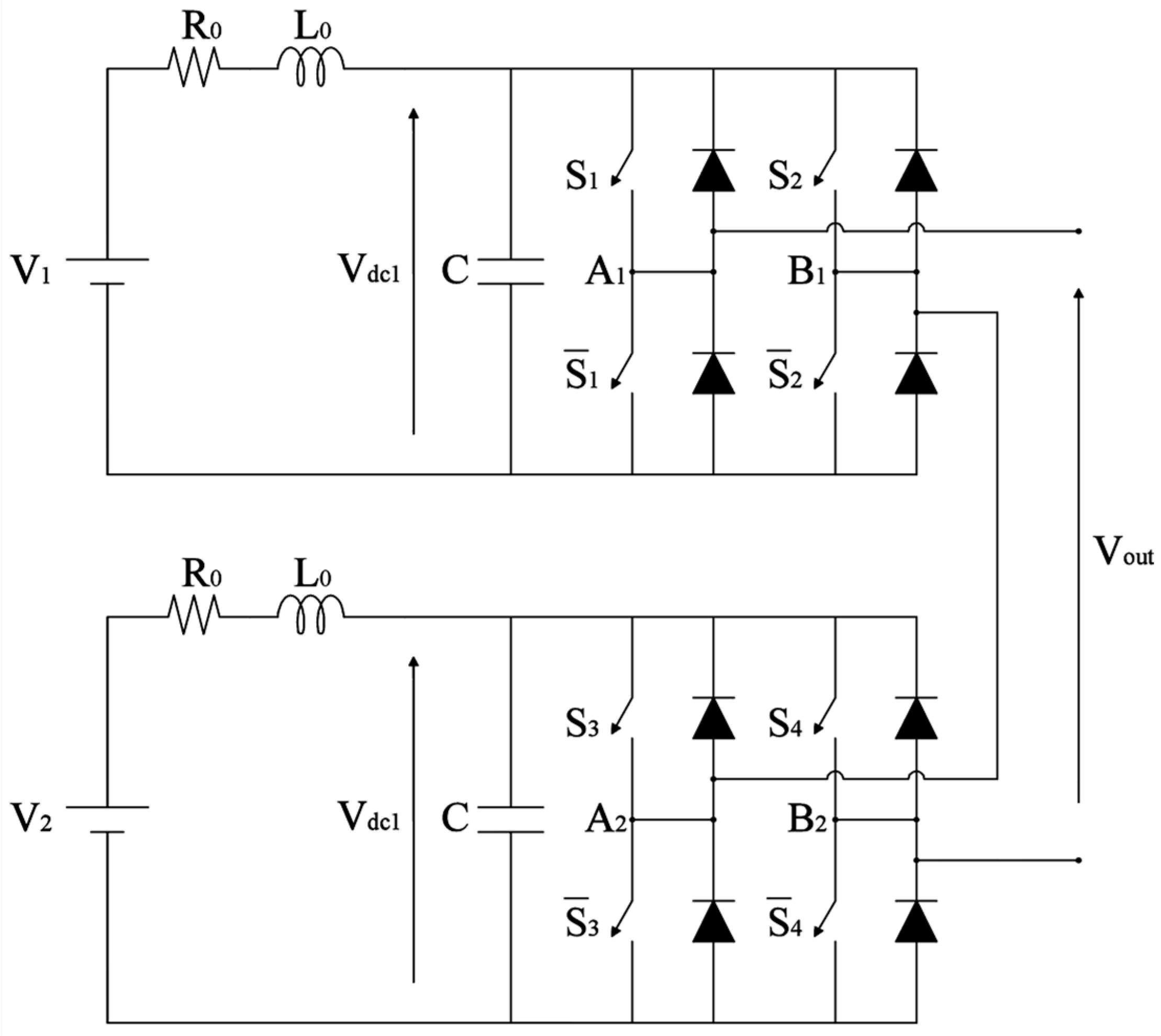
Figure 1 illustrates the topology circuit of the considered single-phase five-level CHBMI. This type of converters has simple circuital structures, made by two H-bridges connected in series and two series of PV panels, obtaining the DC sources. The converter output voltage, Vout, is realized by the states combination of the switches. The switch state can assume only two values, as reported in Equation (1):
With reference to Figure 1, the output voltage Vout of the converter can be expressed as follows:
where Vdc1 and Vdc2 are the DC-link voltage of the two H-bridges connected in series, respectively. In this work, Vdc1 and Vdc2 of Equation (2) have been considered with the same value, equal to Vdc. Thus, Equation (2) can be rewritten in Equation (3).
The possible combinations of the switch states and the output voltage value Vout (t), with reference to Figure 1, are reported in Table 1.
It is interesting to note that there are only two switch state combinations where the output voltage Vout (t) is equal to 2Vdc and −2Vdc, respectively. Furthermore, there are four switch state combinations to obtain an output voltage equal to Vdc, −Vdc, and zero.
3. Voltage Waveform Analysis
The output voltage waveform of the inverter, as previously mentioned, can be obtained through the arrangements of the states of the switches. Thus, every arrangement synthesizes only one voltage level. By the analysis of Equation (3), the voltage waveforms can be obtained through a separate control of the H-bridge connected in series. Thus, it is possible control the time duration of the voltage level separately.
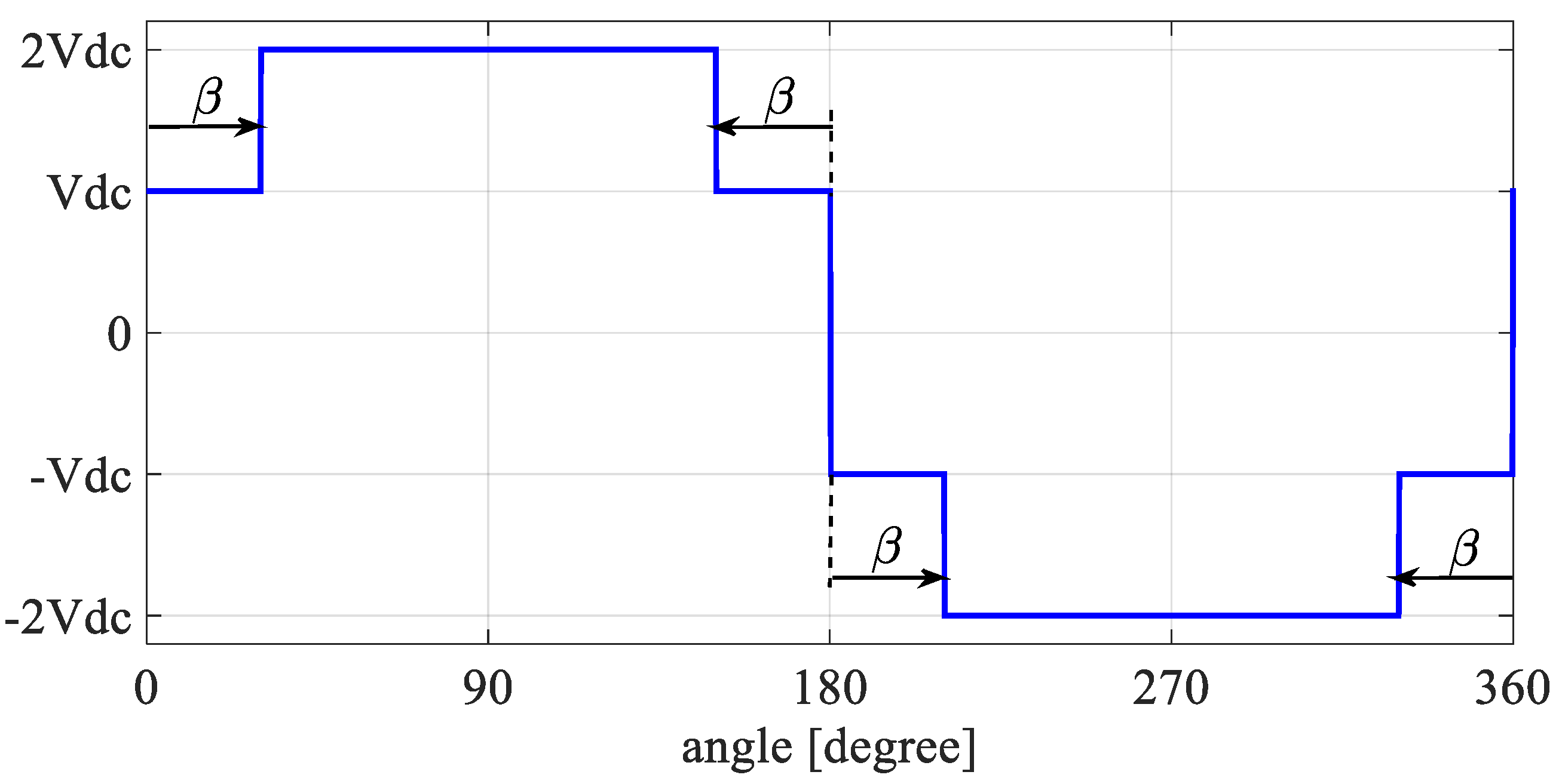
In order to evaluate the harmonic content of the voltage output of a single-phase five-level CHBMI, a square waveform with amplitude equal to 4Vdc peak to peak was taken into account. Moreover, it is essential to outline the parameter β that represents the width of angular range, where the amplitude of the output voltage is equal to Vdc, as shown in Figure 2. The reference square waveform, with 4Vdc peak to peak, can be obtained with β = 0.
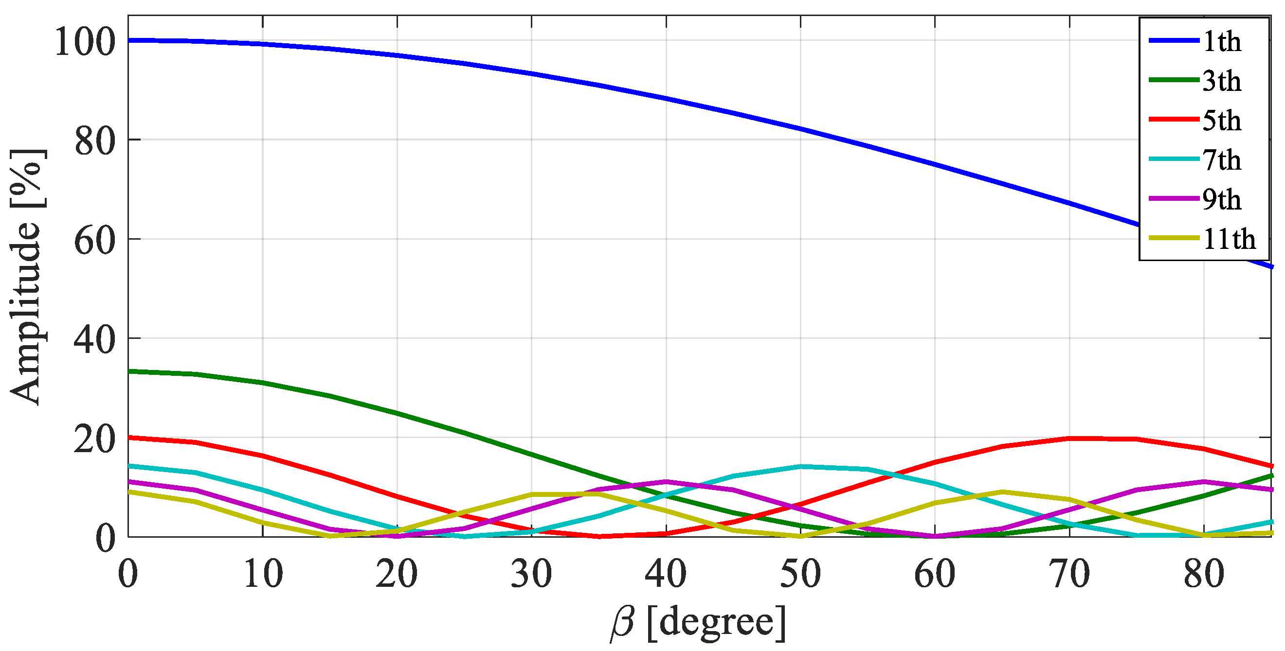
The addition of a stepped voltage level, because β ≠ 0, causes a variation in the harmonic content in the output voltage compared with the reference square waveform. Figure 3 shows the amplitude trend of fundamental harmonic (blue curve), third harmonic (green curve), fifth harmonic (red curve), seventh harmonic (cyan curve), ninth harmonic (purple curve), and eleventh harmonic (yellow curve) versus β expressed in percent respect to the fundamental with β = 0.
As shown in Figure 3, the mutable value of β determines diverse harmonic contents in the output voltage; in particular, there are values of β bringing some harmonic amplitudes to zero. For example, the amplitude of third harmonic is zero for β equal to 60°. Furthermore, it has been noted that the amplitude of fundamental harmonic is reduced with the increase of β and it is not a linear trend.
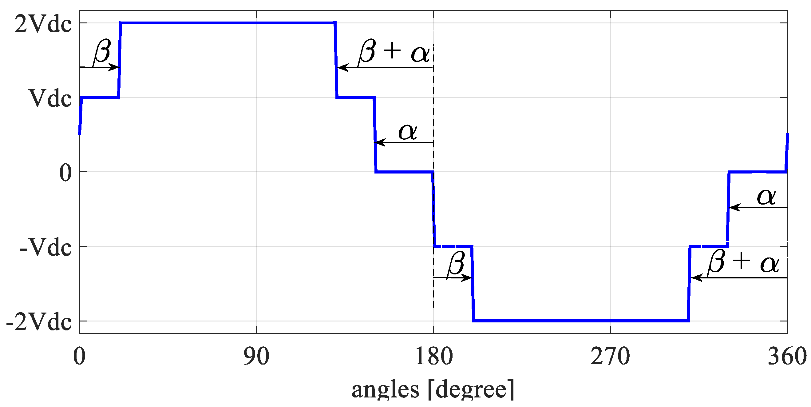
In literature, modulation techniques for a single-phase H-bridge inverter known as “voltage cancellation” are reported [52]. In this work, the same concept as that used for single-level H-bridge inverters has been applied at a single-phase five-level CHBMI, by considering another parameter that can change the harmonic content in output voltage, named α, angular width for which the output voltage is equal to zero, as shown in Figure 4.
The harmonic content of the voltage waveform shown in Figure 4 was studied by means of the Fourier series. Voltage waveform presents half wave symmetry; thus, amplitude values of even harmonics are zero. In Equation (4), the mathematical formulation of the harmonic amplitude Vh and Fourier coefficients Ah and Bh, where h is the harmonic order, were reported.
In Equation (5), the voltage waveform in time domain was reported. Obviously, only for odd values of harmonic order.
More in detail, Equation (6) can be used to determine the amplitude of the fundamental harmonic A1 and the reference harmonics A3–11.
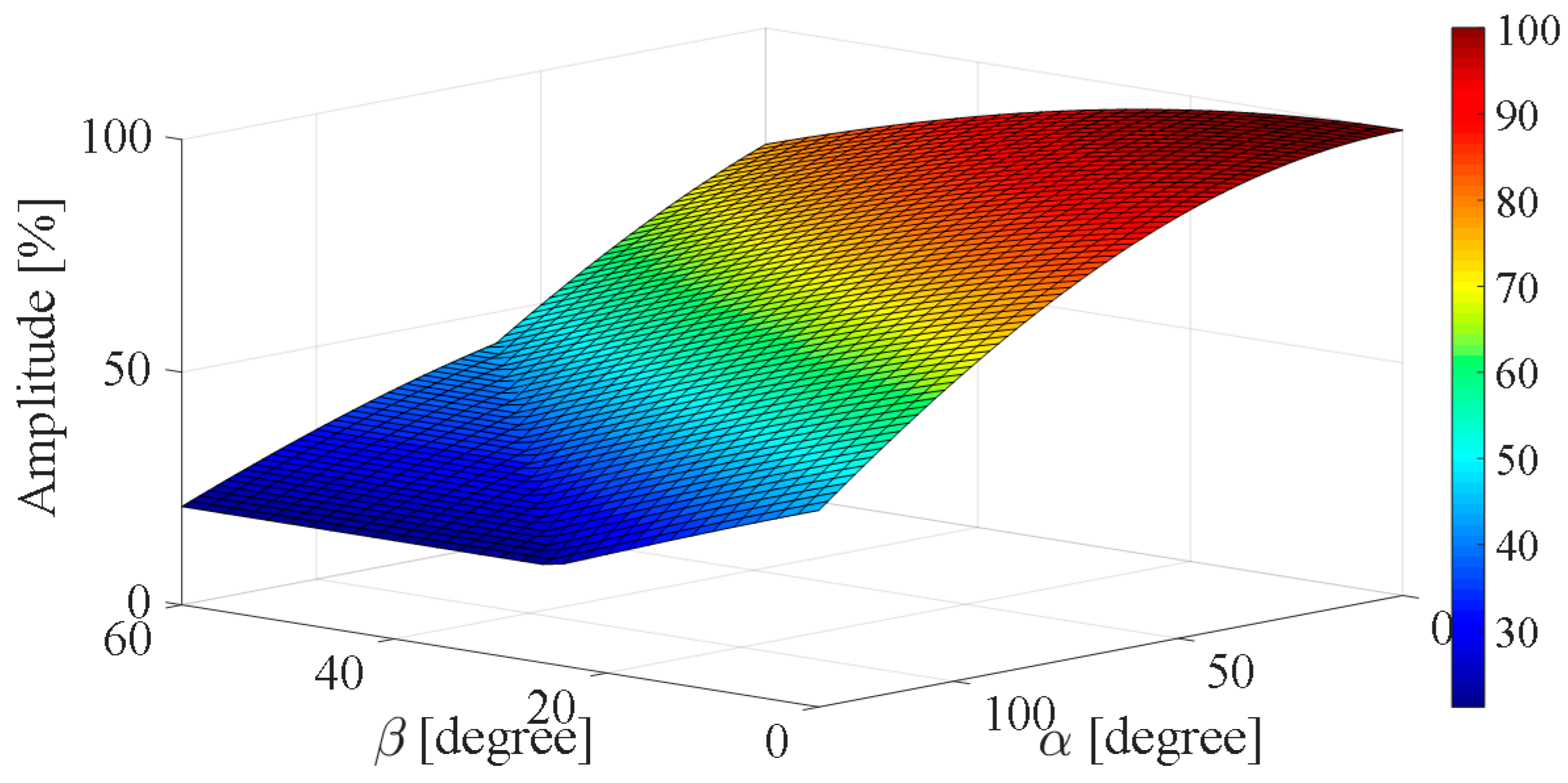
The amplitude of fundamental can be varied with α and β values. Figure 5 shows amplitude trend of fundamental versus α and β expressed in percent respect to the fundamental with α = 0 and β = 0. For big values of α and β, there is a change of slope in the trend amplitude because the converter works with only three voltage levels.
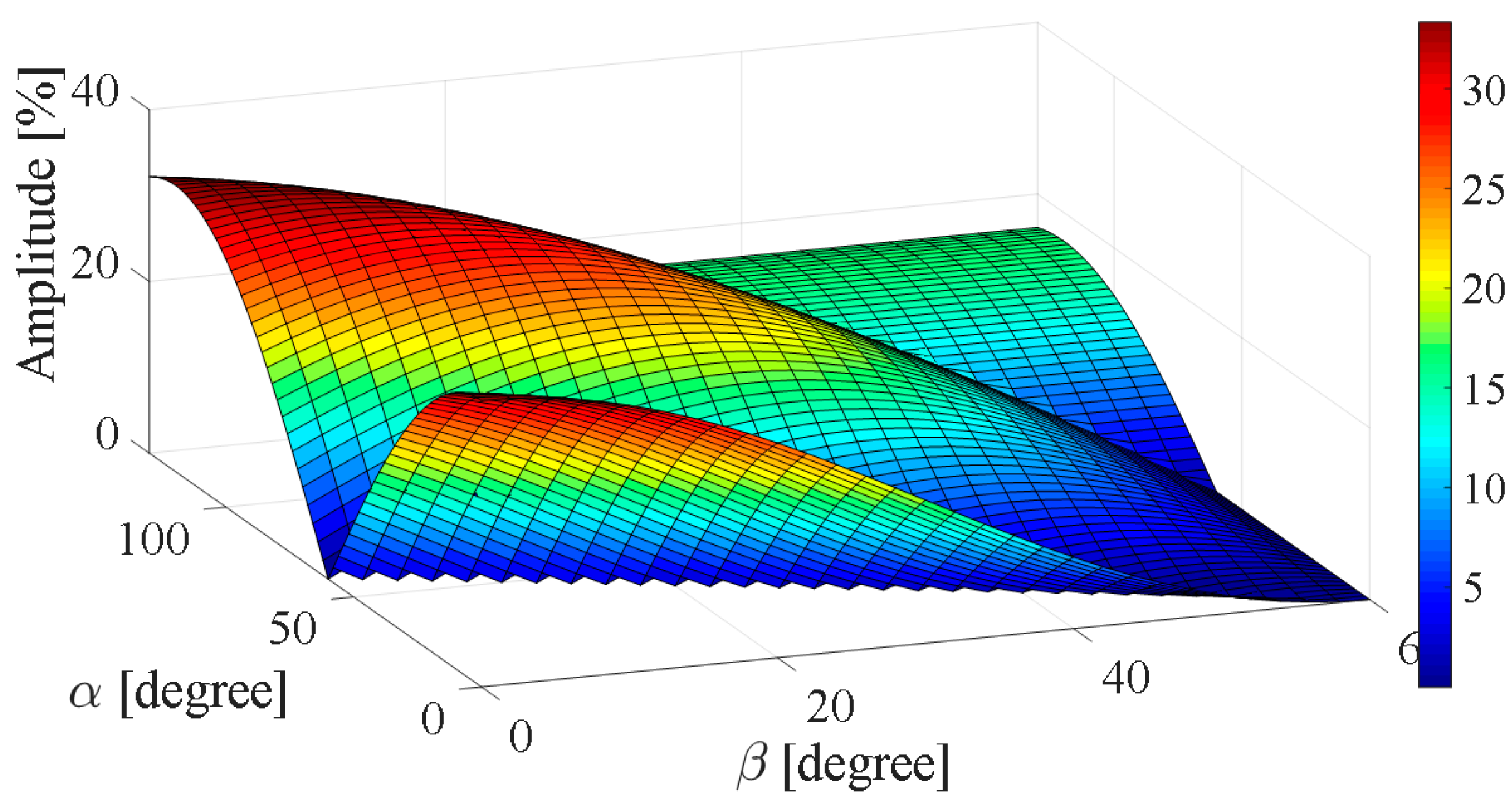
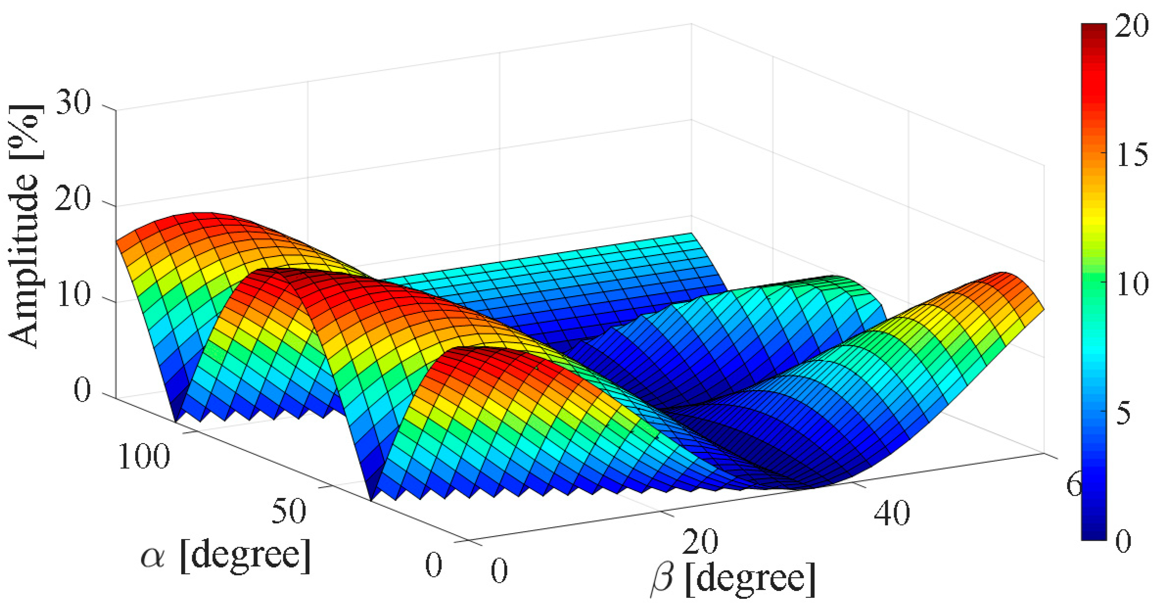
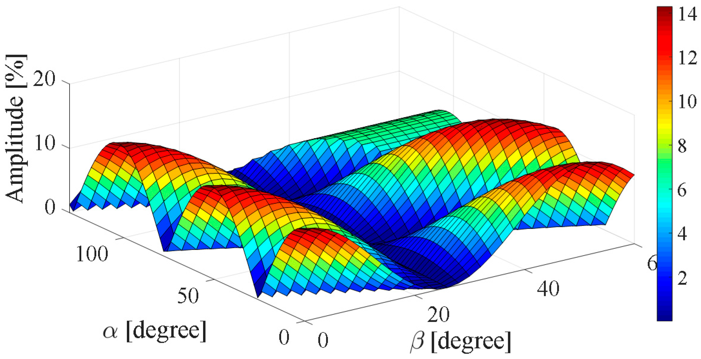
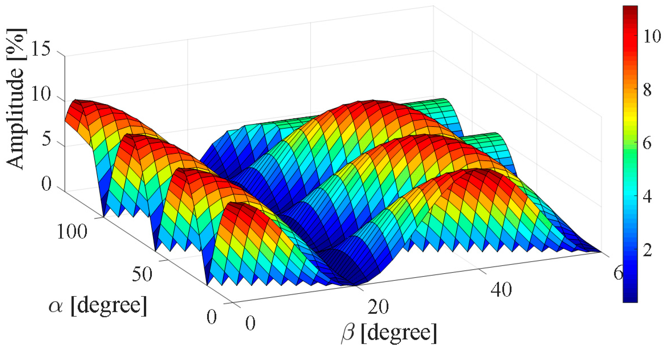
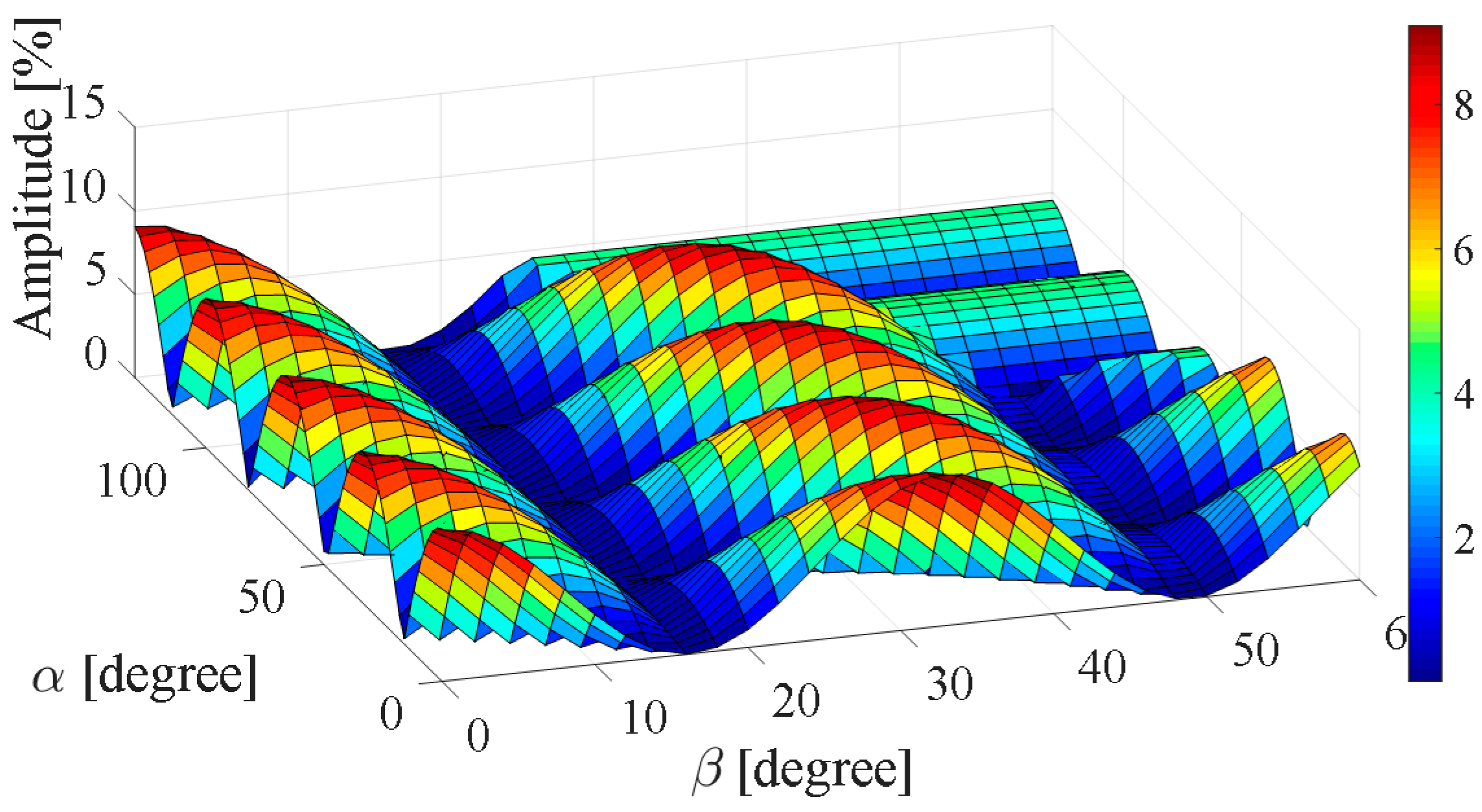
Figure 6, Figure 7, Figure 8, Figure 9 and Figure 10 show the amplitude trend of third, fifth, seventh, ninth, and eleventh harmonics versus α and β expressed in percent respect to the fundamental with α = 0 and β = 0. It is interesting to note that there are values of α and β that concur together to lowering the considered harmonic amplitude. These areas are colored in darker blue.
The objective of the next sections, is to propose a new approach for the harmonics mitigation through the individuation of the “working area” (WA), where it is possible to minimize the reference harmonics (third, fifth, seventh, ninth, and eleventh harmonics) without solving non-linear equations.
4. Mitigation Method of Reference Harmonics
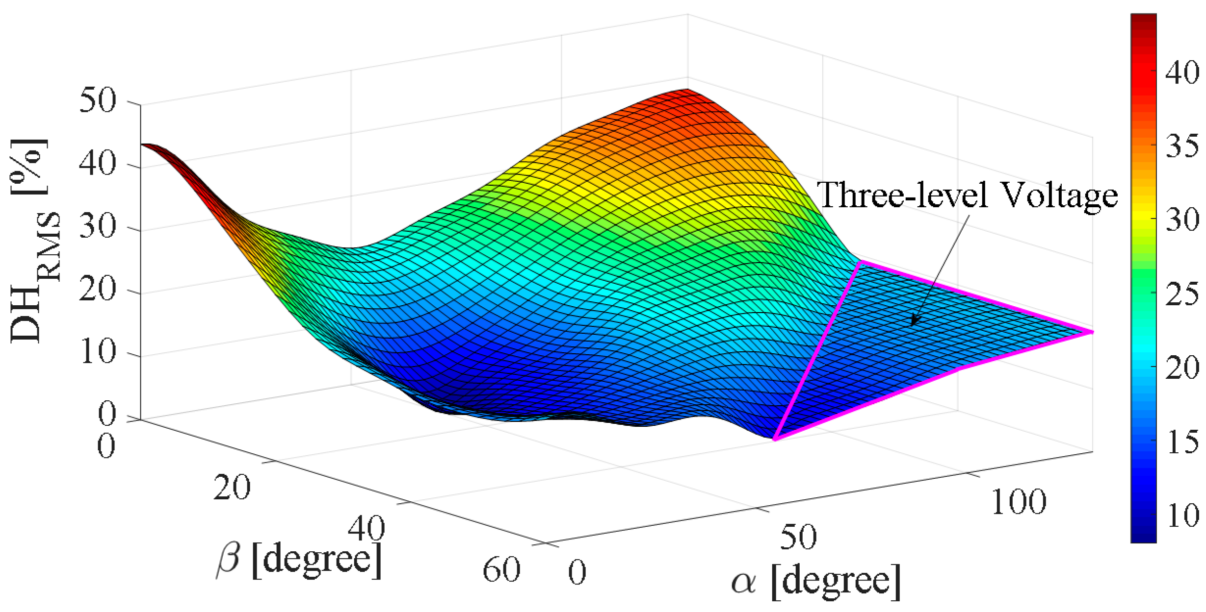
As previously described, the main purpose of this work is the mitigation of reference harmonics without solving non-linear equations. In particular, the proposed method is focused on the research of a working area (WA) where the reference harmonics have the minimum values of the amplitude. For the application of this method, it is necessary to calculate the distorting element (DHRMS) of the voltage waveform, which takes into account only the reference harmonics, through Equation (7). In other words, the DHRMS parameter represents the distorting component of the voltage waveform to be mitigated.
The amplitude of DHRMS is function of the control angles α and β as can be seen in graphic representation in Figure 11.
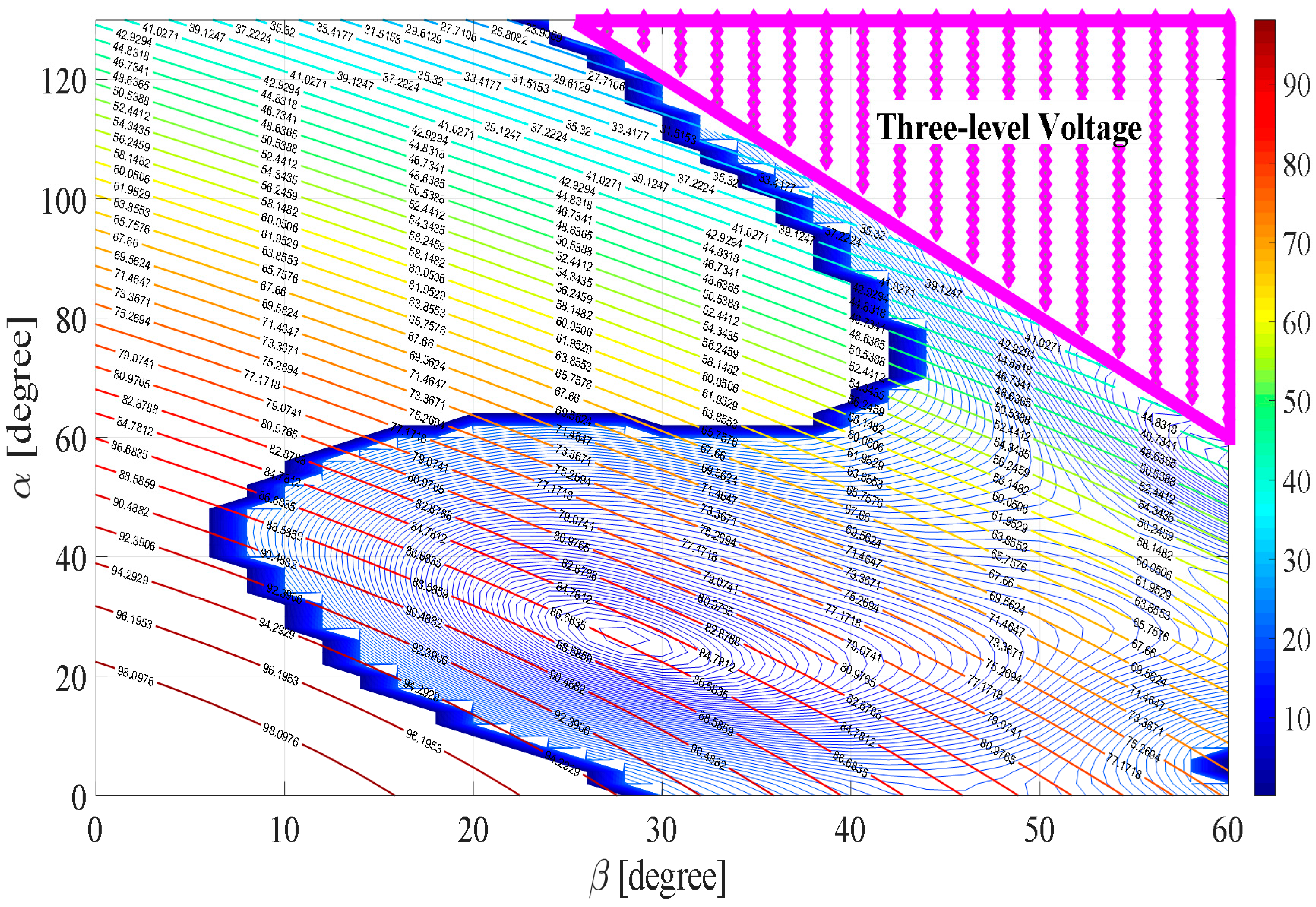
The delimited area with purple lines is the working region where the voltage waveform has only three level voltage. For this reason, this area was neglected for the working points. As can be seen in Figure 11, there is an area with dark blue coloring where the amplitude of the DHRMS is low. Inside this area, it is possible to define the mitigation of reference harmonics. In order to evaluate the WA, a threshold equal to 20% was chosen and through of the level curves the DHRMS and fundamental amplitude were represented. The result obtained is shown in Figure 12.
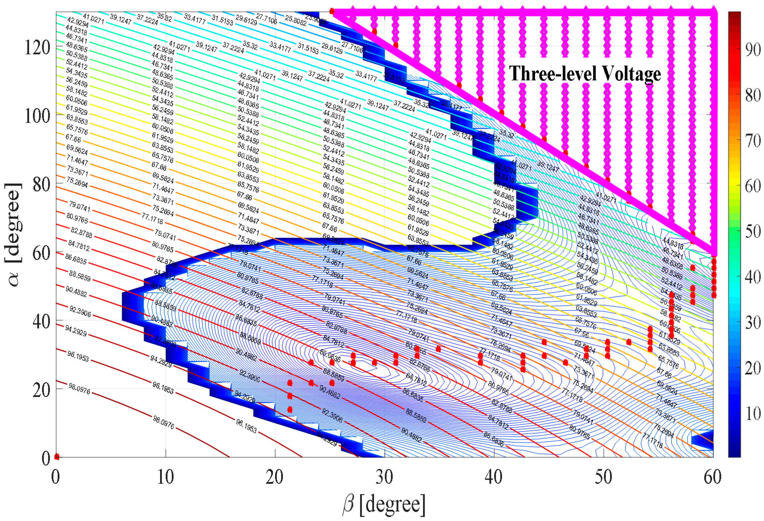
Figure 12 reports the values of DHRMS with a color map, but also the fundamental amplitude with circumference arcs. By the analysis of Figure 12, it is interesting to note that there is a WA, with dark blue coloring, where the maximum variation of the fundamental amplitude is delimited from approximately 42% to 94%. The clear region has higher values of DHRMS (above 20%) so it can be neglected, and the purple region is the one in which the inverter reduces its levels from five to three, and again can be neglected.
The aim of the proposed method is to find the minimum values of the DHRMS for each values of the fundamental amplitude. Thus, the minimum values have to be found in the interceptions of the DHRMS blue lines and circumference arcs of the fundamental amplitude. Therefore, it is possible detected the minimum values of DHRMS and the corresponding control angles, as shown in Figure 13.
The red dots, shown in Figure 13, represent the trajectory of the minimums values of DHRMS. For each minimum value of DHRMS, there is a pair of value of control angles α and β. In this way, it is possible to obtain mitigation for the chosen harmonic, but the control angles are known without continuity inside the WA. The aim of the next section is to find polynomial equations for the real-time operation of the converter. In this way, all values that reduce the fundamental amplitude from 42% to 94% can be obtained.
5. Polynomial Equations for Real-Time Operation
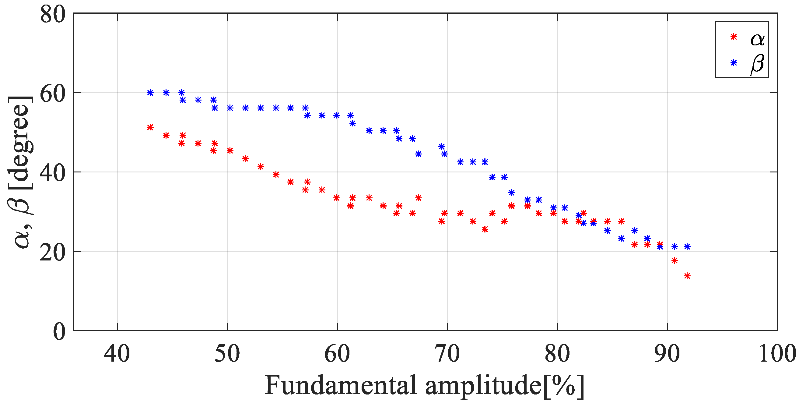
As stated previously, a WA that minimizes the DHRMS of the considered harmonics was identified. Moreover, for each value of the fundamental amplitude, the minimum values of the DHRMS were detected and are represented as red dots in Figure 13. Thus, the control angles versus the fundamental amplitude in the range from 42% to 94% have been determined, as shown in Figure 14.
For real-time operation, it is necessary to know a continuous trend of the control angles α and β inside the WA. Thus, polynomial equations for approximating the trend were evaluated. All equations present a parameter A, indicated in percentage of 100·(π/(8·Vdc)), which represents the amplitude reference of the voltage waveform. The following five cases, approximating the control angles trends, were taken into account.
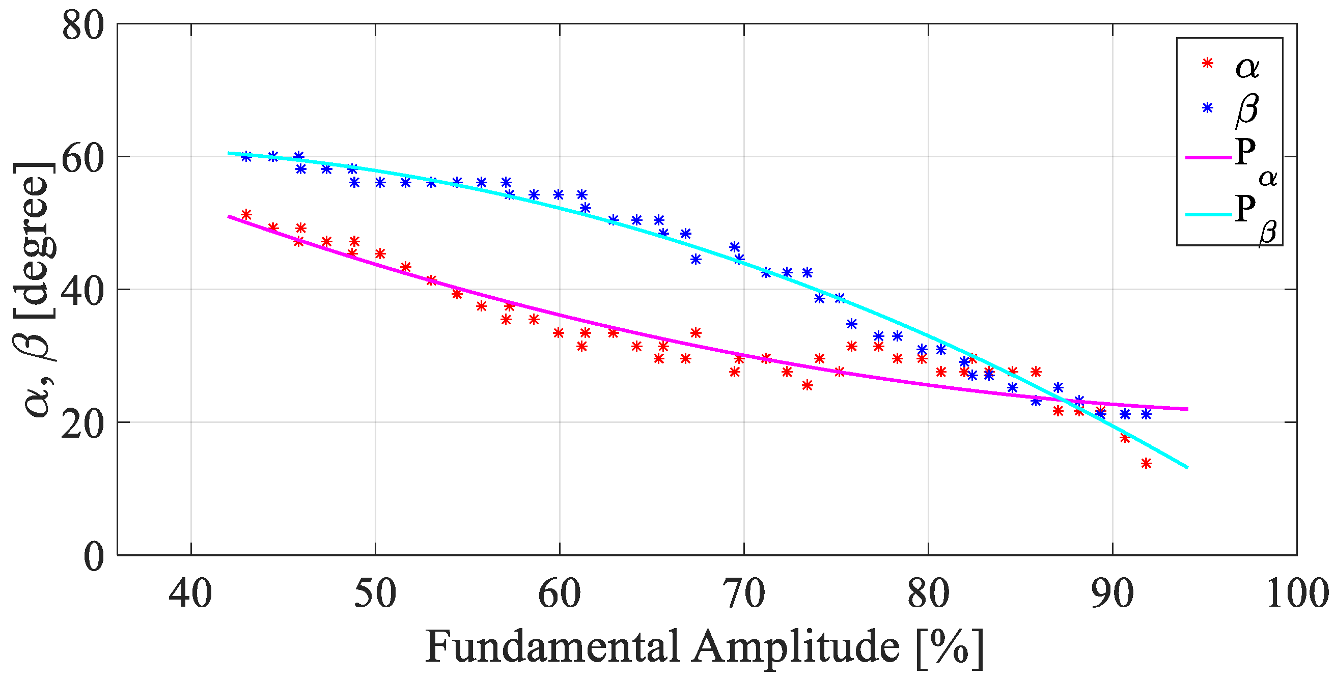
In case 1, two second-order polynomial approximations Pα and Pβ were used, as shown in Figure 15 and reported in Equation (8):
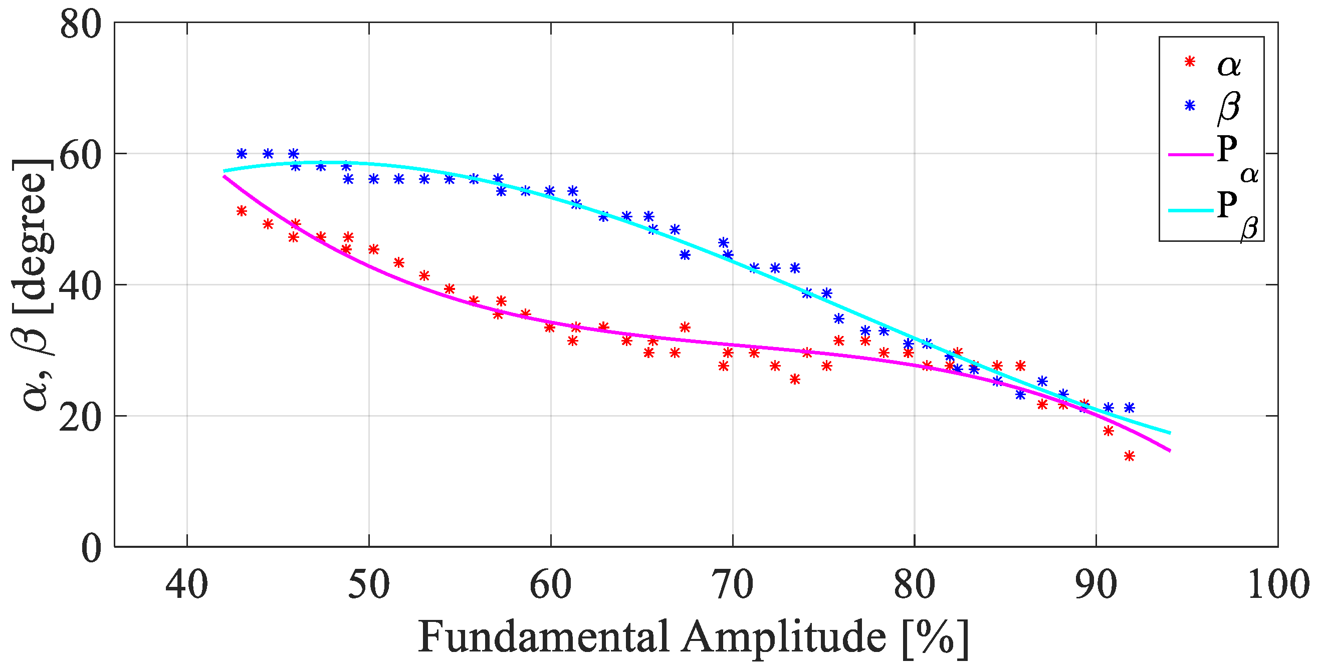
In case 2, the following two third-order polynomial equations Pα and Pβ have been used, and compared with valued that reduce the DHRMS, as shown in Figure 16.
In case 3, the range of variation fundamental amplitude, from 42% to 94%, was split into two parts. The first one section involves the variation of the fundamental amplitude from to 42% to 76% and the second section involves the one from 76% to 94%.
For both intervals, two second-order polynomial equations, Pα1 and Pβ1 for the first section and Pα2 and Pβ2 for the second section, were used. Figure 17 shows approximation of case 3.
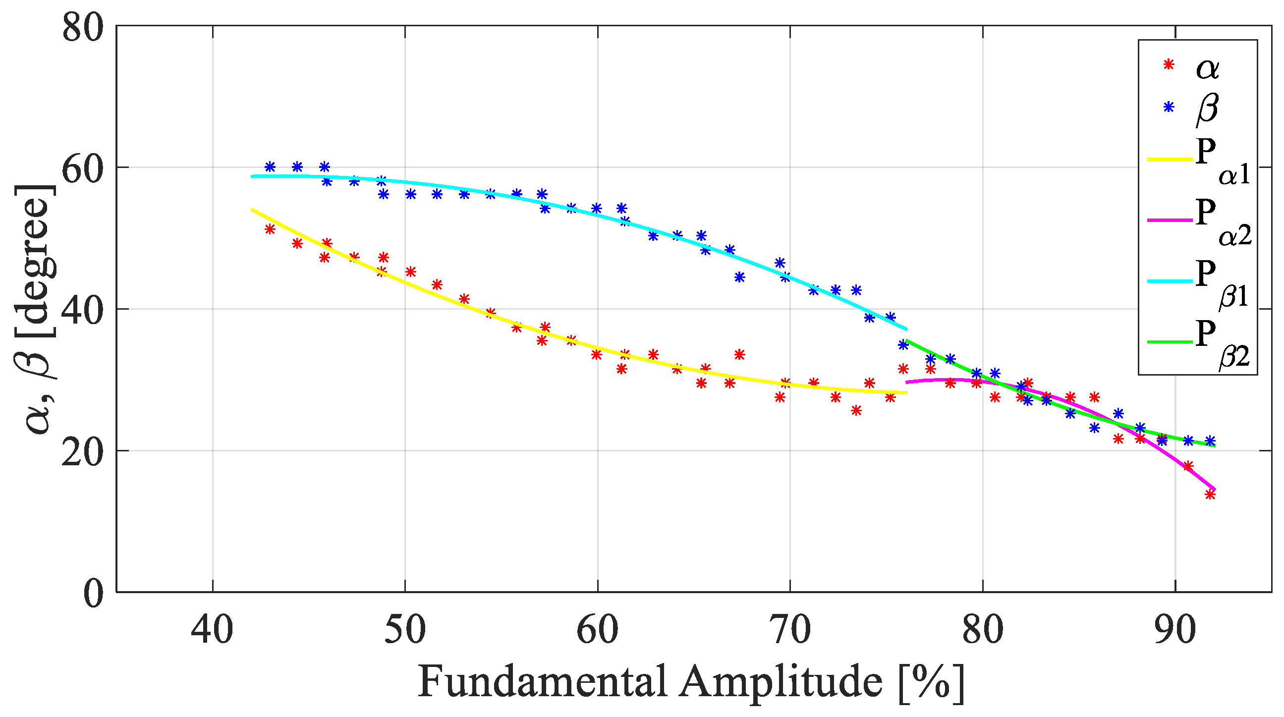
In case 4, the range of variation of the fundamental amplitude, as made for case 3, has been split into two intervals. For the first section, two second-order polynomial equations Pα1 and Pβ1 have been used, while for the second section, two third-order polynomial equations Pα2 and Pβ2 were used. Figure 18 shows the reconstruction of case 4.
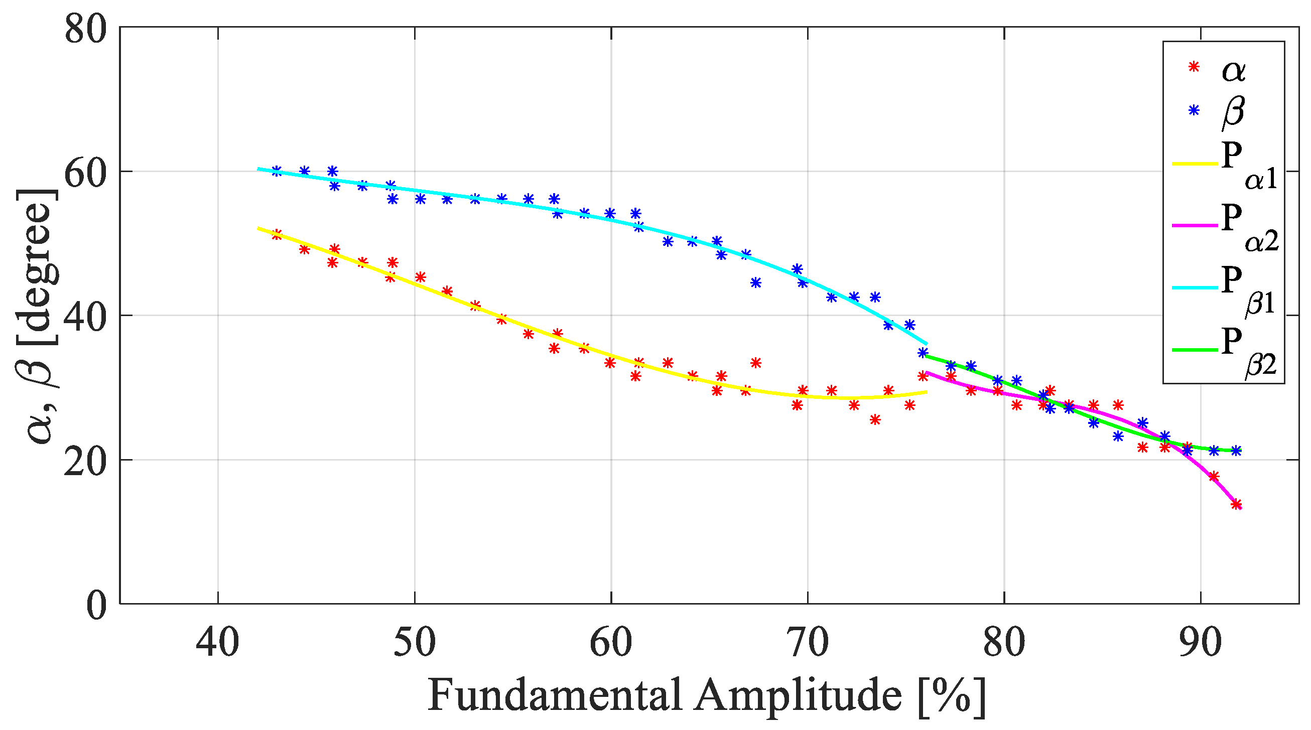
Also, for case 5, the range of variation of the fundamental amplitude was split into two sections. For both sections, two third-order polynomial equations, Pα1 and Pβ1 for the first section and Pα2 and Pβ2 for the second section, have been used. Figure 19 shows the reconstruction for case 5.
The evaluation of the performance for the five cases was carried out. The aim of the simulations is to reproduce the performances of the converter using the polynomial equations, to evaluate the control angles, as previously described. In Matlab/Simulink® (version 4.1.1, The MathWorks, Inc., Natick, MA, USA) environment mathematic model of the single-phase CHBMI, polynomial equations and logic circuit to generate the gate signals were implemented.
The used tool to compare the performances of the converter, employing different polynomial equations to evaluate the control angles α and β, is the total harmonic distortion rate, THD%, as defined in Equation (13), where Vrms is the root mean square value of the voltage waveform and Vrms,1 is the root mean square of the fundamental amplitude [53].
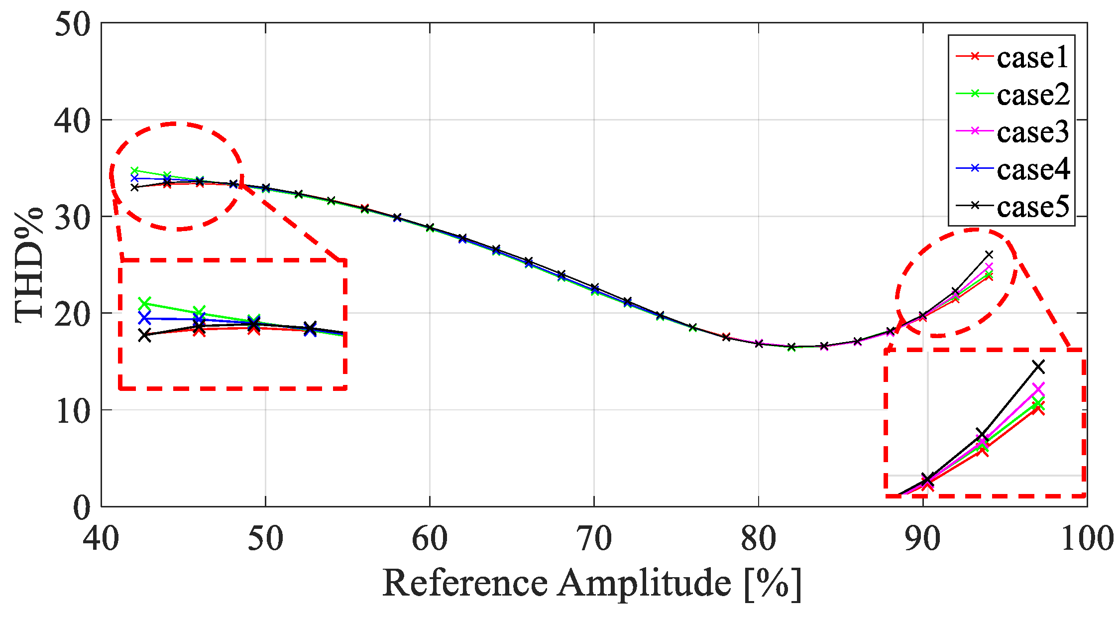
Figure 20 shows comparison among different THD% values obtained for the five different cases. It is interesting to note that in the center of the range, the THD% values are similar for the different cases. Whereas there are different values in the extreme values of the range. In particular, case 1 (red curve) presents the lower values, as illustrated in Figure 20. For this reason, the polynomial equations obtained in case 1 represent the best choice; in real time operation, case 1 requires the lower time execution algorithm respect other cases presented, and it also contributes to better approximating the WA by evaluating the THD%.
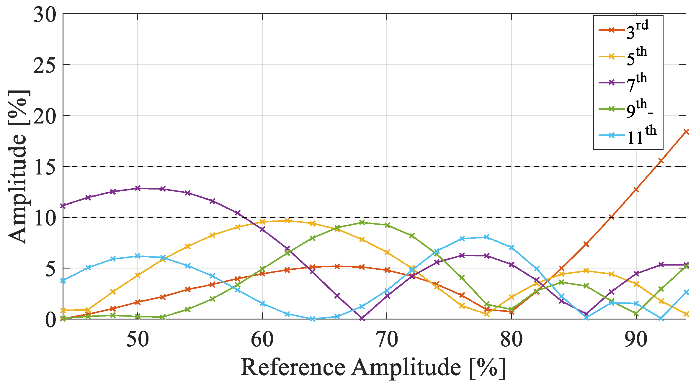
Figure 21 shows the amplitudes of the obtained reference harmonics. By considering the fundamental amplitude variation from 60% to 88%, the amplitude of the reference harmonics is lower than 10%. The seventh harmonic has the amplitude higher than 10% in the range from 44% to 60%. While, the amplitude of the third harmonic increases after 88% of the reference amplitude.
In the next section, an experimental validation of the simulation results was reported. The experimental validation has been carried out by considering only the polynomial equations of case 1.
6. Experimental Validation and Discussion
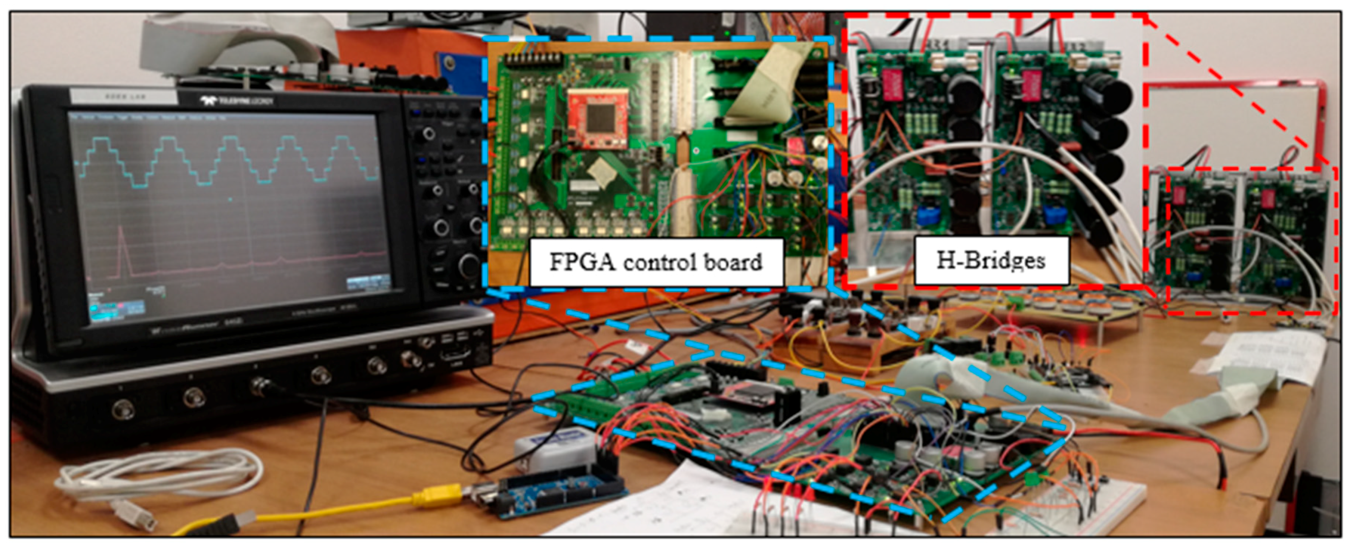
The aim of this paragraph is to reproduce experimentally the results obtained in the Simulink environment. A single-phase, five level DC/AC converter prototype with a CHBMI circuital structure has been assembled in order to carry out the experimental analysis. The test bench is shown in Figure 22.
By means of the described test bench, the proposed technique was experimentally tested. The control algorithm was implemented by mean a prototype of FPGA-based (Altera Cyclone III) control board. The use of a FPGA allows the fast execution of control algorithms, parallel elaborations, high numbers of I/O, and high flexibility.
The mathematical operations are managed by a clock signal with frequency equal to 100 MHz and the resolution choice is 32 bit at floating point. The evaluation of the control angles α and β was carried out in 1.01 μs. For the gate signals generation, a simple logic circuit was implemented.
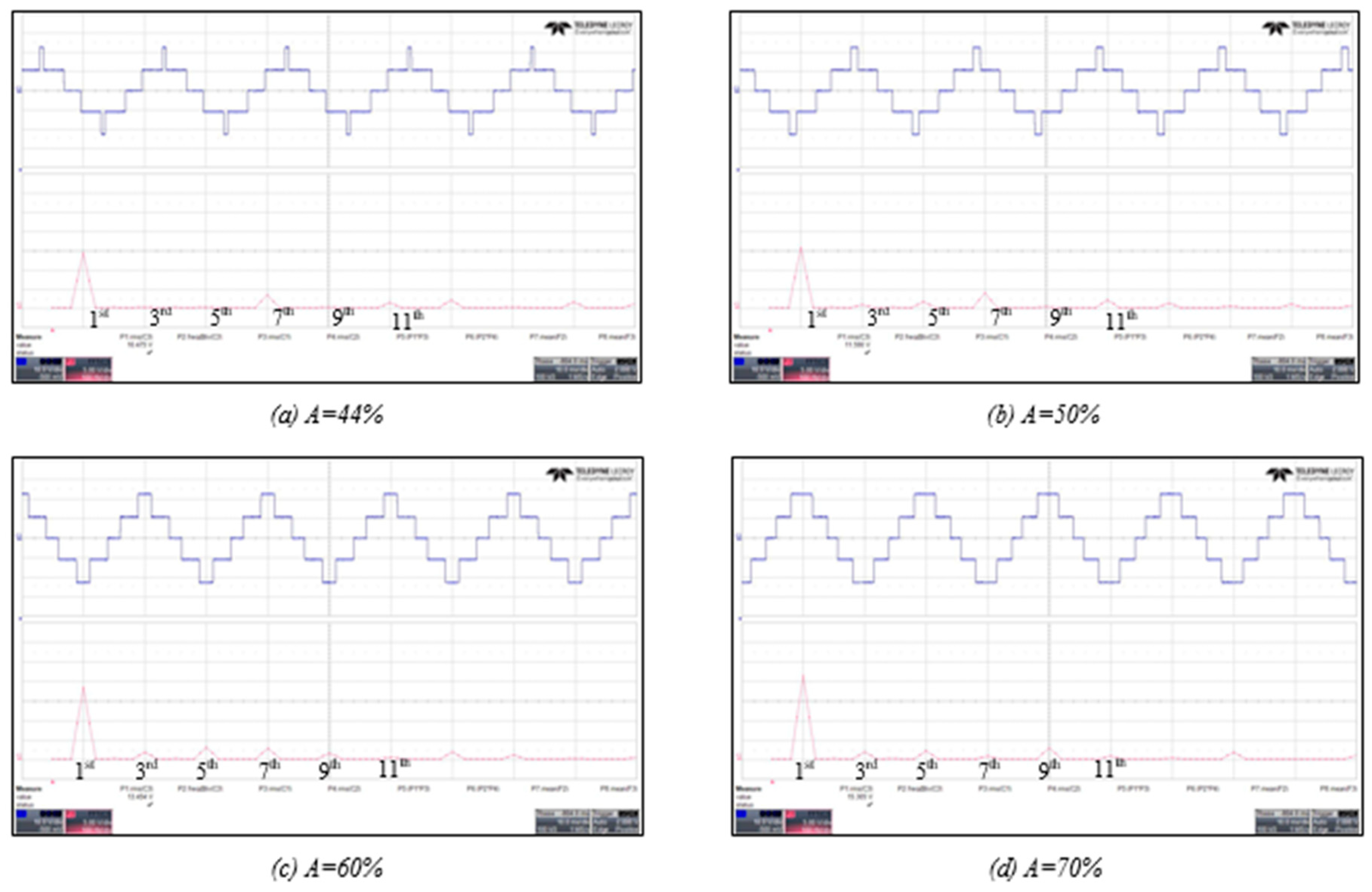
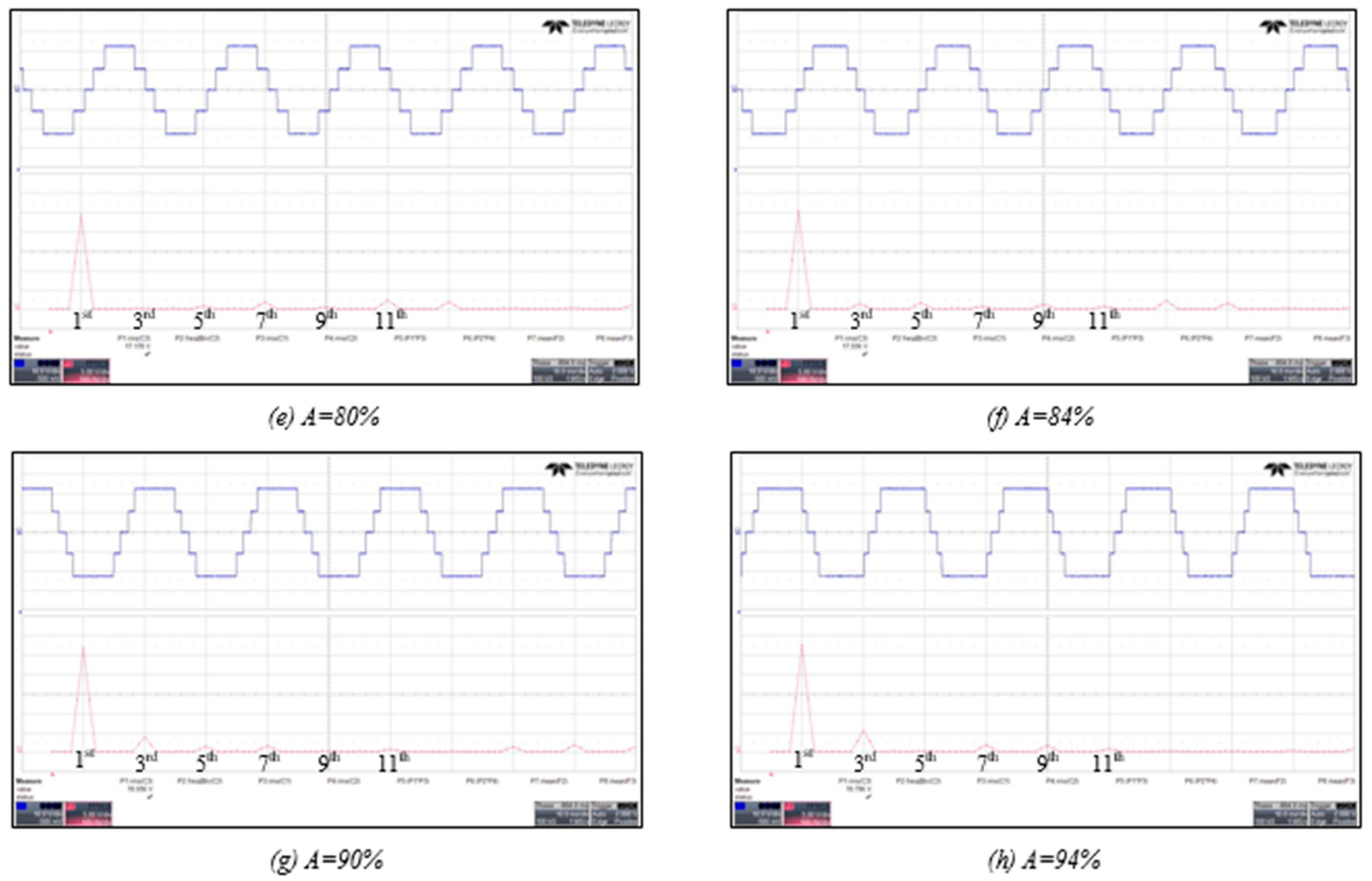
The voltage waveforms have been acquired by the acquisition system with a number of samples equal to 0.5 Ms and in a time interval equal to 20 ms. The acquired experimental samples of the voltage waveforms were processed in Matlab® environment. Figure 23 shows the screenshots of the acquired voltage waveforms and corresponding harmonic spectra for some values of reference amplitude A.
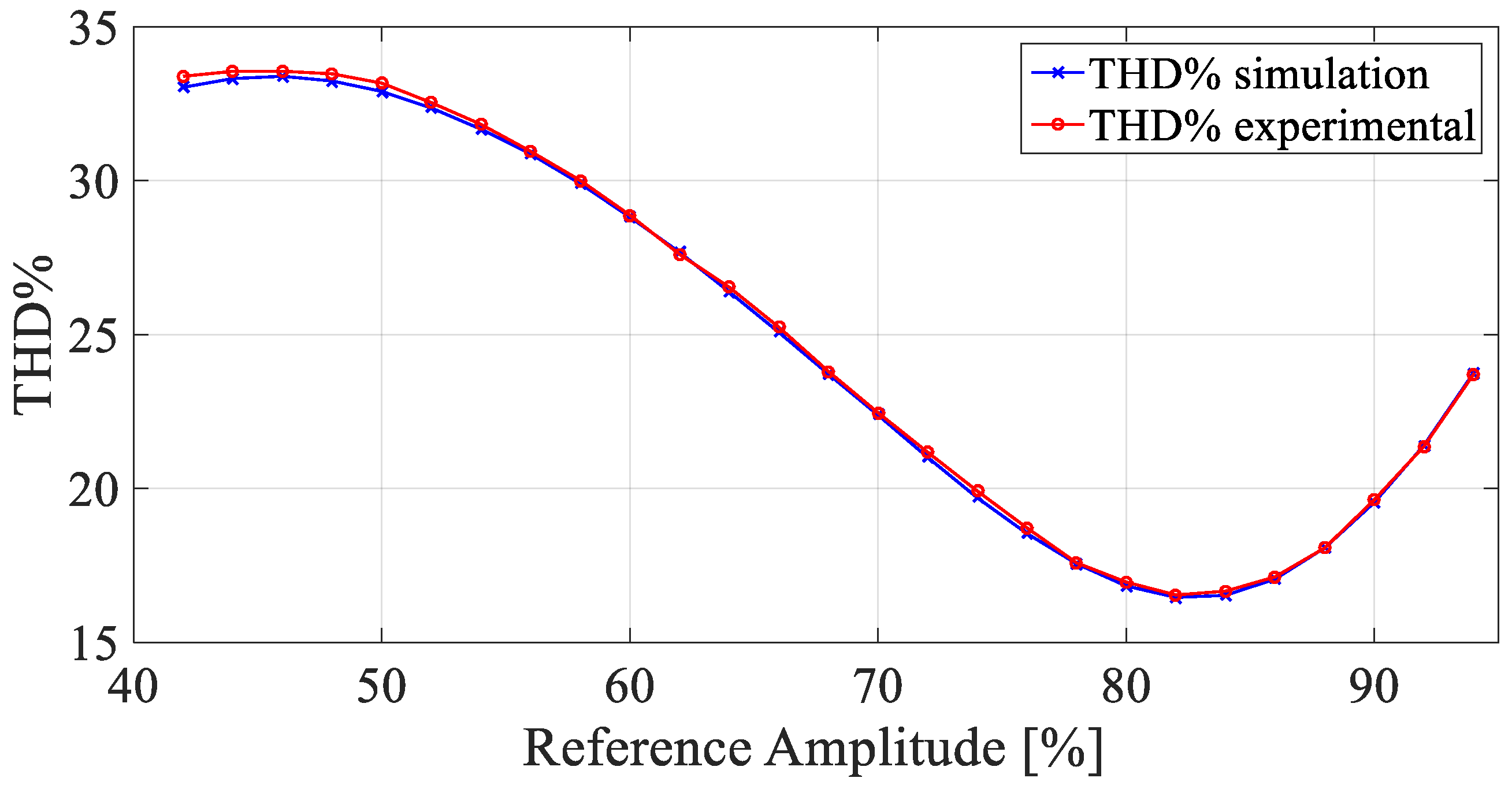
The used tool to compare the experimental tests with simulations is THD%. Figure 24 shows the comparison between THD% obtained by simulation analysis (blue curve) and THD% obtained by experimental tests (red curve). It is interesting to note that the experimental THD% presents similar values with respect to the simulated ones. In particular, there are only small differences for low values of the reference amplitude.
For reference amplitude equal to 46%, there is the maximum value of THD% equal to 33.55%. In the range of reference amplitude from 74% to 90%, there are lower values, about 20%. For reference amplitude equal to 82%, there is the minimum value of THD%, which is equal to 16.54%. Such a value is above the proposed ones in the literature [16,19,44,45], but it is obtained for a very simple and more economic structure.
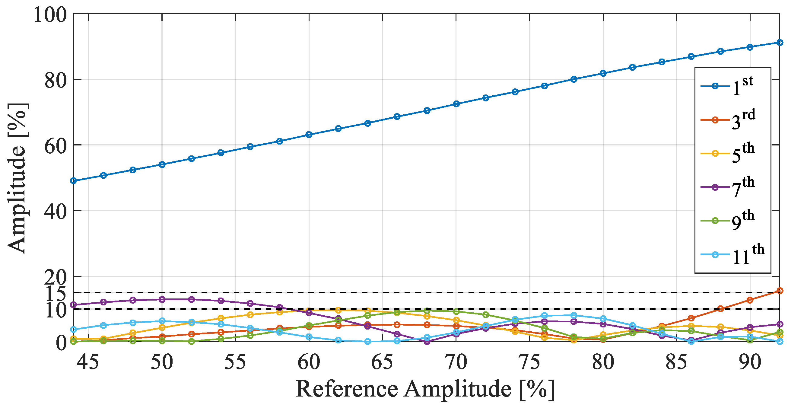
Figure 25 shows the amplitude of fundamental and reference harmonics versus reference amplitude. As observed for simulation results, in the range of reference amplitude from 60% to 88% the amplitude of the reference harmonics is lower than 10%. Moreover, also for the experimental results, there are the same phenomena for the seventh and third harmonics already observed in the simulation results. The fundamental amplitude presents a linear trend inside the working area.
7. Conclusions
This paper presents an alternative way to obtain harmonic mitigation for single-phase five-level CHBMI without solving non-linear equation applied in PV systems. Firstly, the so-called “voltage cancellation” technique has been presented, jointly with the analytical expression of the harmonic content on the voltage waveforms.
The proposed method, through the analysis of the distorting component called DHRMS, detects a working area, in which the mitigation of third, fifth seventh, ninth, and eleventh harmonics can be enforced. Thus, through the evaluation of the minimum points of the DHRMS, the corresponding control angles have been obtained. Moreover, the values of the control parameters can be obtained without solving a set of nonlinear transcendental equations, but through a low-time-consuming polynomial equations implementation. In this way, it is possible to enforce a real-time operation with very low computational costs. By experimental validation, the equations obtained allow to drive the converter only in a definite working area, where it is possible change the reference fundamental amplitude from 44% to 94%. Inside this working area, the harmonics mitigation has been limited under 10% in the range from 62% to 88% of the reference amplitude; the seventh harmonic has the amplitude higher than 10% in the range from 44% to 60%, while the amplitude of the third harmonic increases over 10% when the reference amplitude exceeds the 88%.
Author Contributions
The authors have contributed equally to this work. The authors of this manuscript jointly have conceived the theoretical analysis, modeling, simulation and obtained the experimental data.
Funding
This research received no external funding.
Acknowledgments
This work was financially supported by MIUR-Ministero dell’Istruzione dell’Università e della Ricerca (Italian Ministry of Education, University and Research), by SDESLab (Sustainable Development and Energy Saving Laboratory), and LEAP (Laboratory of Electrical Applications) of the University of Palermo.
Conflicts of Interest
The authors declare no conflict of interest.
References
- Directive 2010/31/EU of the European Parliament and of the Council of 19 May 2010 on the Energy Performance of Buildings. Available online: http://www.buildup.eu/en/practices/publications/directive-201031eu-energy-performance-buildings-recast-19-may-2010 (accessed on 15 January 2018).
- Miceli, R.; Viola, F. Designing a sustainable university recharge area for electric vehicles: Technical and economic analysis. Energies 2017, 10, 1604. [Google Scholar] [CrossRef]
- Prabaharan, N.; Palanisamy, K. A comprehensive review on reduced switch multilevel inverter topologies, modulation techniques and applications. Renew. Sustain. Energy Rev. 2017, 76, 1248–1282. [Google Scholar] [CrossRef]
- Baker, R.H.; Bannister, L.H. Electric Power Converter. U.S. Patent 3867643, 16 February 1975. [Google Scholar]
- Yuan, X.; Barbi, I. Fundamentals of a new diode clamping multilevel inverter. IEEE Trans. Power Electron. 2000, 15, 711–718. [Google Scholar] [CrossRef]
- Rodriguez, J.; Bernet, S.; Steimer, P.K.; Lizama, I.E. A survey on neutral-point-clamped inverters. IEEE Trans. Ind. Electron. 2010, 57, 2219–2230. [Google Scholar] [CrossRef]
- Huang, J.; Corzine, K.A. Extended operation of flying capacitor multilevel inverters. IEEE Trans. Power Electron. 2006, 21, 140–147. [Google Scholar] [CrossRef]
- Kou, X.; Corzine, K.A.; Wielebski, M.W. Overdistention operation of cascaded multilevel inverters. IEEE Trans. Ind. Appl. 2006, 42, 817–824. [Google Scholar]
- Kala, P.; Arora, S. A comprehensive study of classical and hybrid multilevel inverter topologies for renewable energy applications. Renew. Sustain. Energy Rev. 2017, 76, 905–931. [Google Scholar] [CrossRef]
- Venkataramanaiah, J.; Suresh, Y.; Panda, A.K. A review on symmetric, asymmetric, hybrid and single DC sources based multilevel inverter topologies. Renew. Sustain. Energy Rev. 2017, 76, 788–812. [Google Scholar] [CrossRef]
- Jana, J.; Saha, H.; Bhattacharya, K.D. A review of inverter topologies for single-phase grid-connected photovoltaic systems. Renew. Sustain. Energy Rev. 2017, 72, 1256–1270. [Google Scholar] [CrossRef]
- Monica, P.; Kowsalya, M. Control strategies of parallel operated inverters in renewable energy application: A review. Renew. Sustain. Energy Rev. 2016, 65, 885–901. [Google Scholar] [CrossRef]
- Kumar, N.; Saha, T.K.; Dey, J. Modeling, control and analysis of cascaded inverter based grid-connected photovoltaic system. Int. J. Electr. Power Energy Syst. 2016, 78, 165–173. [Google Scholar] [CrossRef]
- Ravi, A.; Manoharan, P.S.; Anand, J.V. Modeling and simulation of three phase multilevel inverter for grid connected photovoltaic systems. Sol. Energy 2011, 85, 2811–2818. [Google Scholar] [CrossRef]
- Rajkumar, M.V.; Manoharan, P.S. FPGA based multilevel cascaded inverters with SVPWM algorithm for photovoltaic system. Sol. Energy 2013, 87, 229–245. [Google Scholar] [CrossRef]
- Prabaharan, N.; Palanisamy, K. Analysis and integration of multilevel inverter configuration with boost converters in a photovoltaic system. Energy Convers. Manag. 2016, 128, 327–342. [Google Scholar] [CrossRef]
- Iero, D.; Carbone, R.; Carotenuto, R.; Felini, C.; Merenda, M.; Pangallo, G.; Della Corte, F.G. SPICE modelling of a complete photovoltaic system including modules, Energy storage elements and a multilevel inverter. Sol. Energy 2014, 107, 338–350. [Google Scholar] [CrossRef]
- Javad, O.; Shayan, E.; Ali, M. Compensation of voltage sag caused by partial shading in grid-connected PV system through the three-level SVM inverter. Sustain. Energy Technol. Assess. 2016, 18, 107–118. [Google Scholar]
- Prabaharan, N.; Palanisamy, K. A Single Phase Grid Connected Hybrid Multilevel Inverter for Interfacing Photo-voltaic System. Energy Procedia 2016, 103, 250–255. [Google Scholar] [CrossRef]
- Husev, O.; Roncero-Clemente, C.; Romero-Cadaval, E.; Vinnikov, D.; Jalakas, T. Three-level three-phase quasi-Z-source neutral-point-clamped inverter with novel modulation technique for photovoltaic application. Electr. Power Syst. Res. 2016, 130, 10–21. [Google Scholar] [CrossRef]
- Lauria, D.; Coppola, M. Design and control of an advanced PV inverter. Sol. Energy 2014, 110, 533–542. [Google Scholar] [CrossRef]
- Hannan, M.A.; Azidin, F.A.; Mohamed, A. Hybrid electric vehicles and their challenges: A review. Renew. Sustain. Energy Rev. 2014, 29, 135–150. [Google Scholar] [CrossRef]
- Zhai, L.; Lee, G.; Gao, X.; Zhang, X.; Gu, Z.; Zou, M. Impact of Electromagnetic Interforance from Power Inverter Drive System on Batteries in Electric Vehicle. Energy Procedia 2016, 88, 881–888. [Google Scholar] [CrossRef]
- Mese, E.; Ayaz, M.; Tezcan, M.M. Design considerations of a multitasked electric machine for automotive applications. Electr. Power Syst. Res. 2016, 131, 147–158. [Google Scholar] [CrossRef]
- Tolbert, L.M.; Peng, F.Z.; Cunnyngham, T.; Chiasson, J.N. Charge balance control schemes for cascade multilevel converter in hybrid electric vehicles. IEEE Trans. Ind. Electron. 2002, 49, 1058–1064. [Google Scholar] [CrossRef] [Green Version]
- Khoucha, F.; Lagoun, S.M.; Marouani, K.; Kheloui, A.; Benbouzid, M.E.H. Hybrid cascaded H-bridge multilevel-inverter induction-motor-drive direct torque control for automotive applications. IEEE Trans. Ind. Electron. 2010, 57, 892–899. [Google Scholar] [CrossRef] [Green Version]
- Ding, X.; Du, M.; Zhou, T.; Guo, H.; Zhang, C. Comprehensive comparison between silicon carbide MOSFETs and silicon IGBTs based traction systems for electric vehicles. Appl. Energy 2016, 194, 626–634. [Google Scholar] [CrossRef]
- Kabalyk, Y. Determination of energy loss in power voltage inverters for power supply of locomotive traction motors. Procedia Eng. 2016, 165, 1437–1443. [Google Scholar] [CrossRef]
- Carpita, M.; Marchesoni, M.; Pellerin, M.; Moser, D. Multilevel converter for traction applications: Small-scale prototype tests results. IEEE Trans. Ind. Electron. 2008, 55, 2203–2212. [Google Scholar] [CrossRef]
- Kumar, Y.P.; Ravikumar, B. A simple modular multilevel inverter topology for the power quality improvement in renewable energy based green building microgrids. Electr. Power Syst. Res. 2016, 140, 147–161. [Google Scholar] [CrossRef]
- Kamel, R.M. New inverter control for balancing standalone micro-grid phase voltages: A review on MG power quality improvement. Renew. Sustain. Energy Rev. 2016, 63, 520–532. [Google Scholar] [CrossRef]
- Mohamed, E.E.; Sayed, M.A. Matrix converters and three-phase inverters fed linear induction motor drives-Performance compare. Ain Shams Eng. J. 2016. Available online: https://doi.org/10.1016/j.asej.2016.02.002 (accessed on 21 March 2016).
- Trabelsi, M.; Boussak, M.; Benbouzid, M. Multiple criteria for high performance real-time diagnostic of single and multiple open-switch faults in ac-motor drives: Application to IGBT-based voltage source inverter. Electr. Power Syst. Res. 2017, 144, 136–149. [Google Scholar] [CrossRef]
- Prakash, G.; Subramani, C.; Bharatiraja, C.; Shabin, M. A low cost single phase grid connected reduced switch PV inverter based on Time Frame Switching Scheme. Inter. J. Electr. Power Energy Syst. 2016, 2016 77, 100–111. [Google Scholar] [CrossRef]
- Gupta, V.K.; Mahanty, R. Optimized switching scheme of cascaded H-bridge multilevel inverter using PSO. Inter. J. Electr. Power Energy Syst. 2015, 64, 699–707. [Google Scholar] [CrossRef]
- Mesquita, S.J.; Antunes, F.L.M.; Daher, S. A new bidirectional hybrid multilevel inverter with 49-level output voltage using a single dc voltage source and reduced number of on components. Electr. Power Syst. Res. 2017, 143, 703–714. [Google Scholar] [CrossRef]
- Báez-Fernández, H.; Ramírez-Beltrán, N.D.; Méndez-Piñero, M.I. Selection and configuration of inverters and modules for a photovoltaic system to minimize costs. Renew. Sustain. Energy Rev. 2016, 58, 16–22. [Google Scholar] [CrossRef]
- Schettino, G.; Benanti, S.; Buccella, C.; Caruso, M.; Castiglia, V.; Cecati, C.; Di Tommaso, A.O.; Miceli, R.; Romano, P.; Viola, F. Simulation and experimental validation of multicarrier PWM techniques for three-phase five-level cascaded H-bridge with FPGA controller. Inte. J. Renew. Energy Res. 2017, 7, 1383–1394. [Google Scholar]
- Schettino, G.; Buccella, C.; Caruso, M.; Cecati, C.; Castiglia, V.; Miceli, R.; Viola, F. Overview and experimental analysis of MC SPWM techniques for single-phase five level cascaded H-bridge FPGA controller-based. In Proceedings of the IECON 2016-42nd Annual Conference of the IEEE Industrial Electronics Society, Florence, Italy, 23–26 October 2016; pp. 4529–4534. [Google Scholar]
- Benanti, S.; Buccella, C.; Caruso, M.; Castiglia, V.; Cecati, C.; Di Tommaso, A.O.; Miceli, R.; Romano, P.; Schettino, G.; Viola, F. Experimental analysis with FPGA controller-based of MC PWM techniques for three-phase five level cascaded H-bridge for PV applications. In Proceedings of the 2016 IEEE International Conference on Renewable Energy Research and Applications (ICRERA), Birmingham, UK, 20–23 November 2016; pp. 1173–1178. [Google Scholar]
- Rahim, N.A.; Ping, H.W.; Selvaraj, J. Elimination of harmonics in photovoltaic seven-level inverter with Newton-Raphson optimization. Procedia Environ. Sci. 2013, 2013 17, 519–528. [Google Scholar]
- Kavali, J.; Mittal, A. Analysis of various control schemes for minimal Total Harmonic Distortion in cascaded H-bridge multilevel inverter. J. Electr. Syst. Inf. Technol. 2016, 3, 428–441. [Google Scholar] [CrossRef]
- Al-Othman, A.K.; Abdelhamid, T.H. Elimination of harmonics in multilevel inverters with non-equal dc sources using PSO. In Proceedings of the 2008 13th International Power Electronics and Motion Control Conference (EPE-PEMC 2008), Poznan, Poland, 1–3 September 2008; pp. 756–764. [Google Scholar]
- Ganesan, K.; Barathi, K.; Chandrasekar, P.; Balaji, D. Selective harmonic elimination of cascaded multilevel inverter using BAT algorithm. Procedia Technol. 2015, 21, 651–657. [Google Scholar] [CrossRef]
- Marzoughi, A.; Imaneini, H.; Moeini, A. An optimal selective harmonic mitigation technique for high power converters. Inter. J. Electr. Power Energ. Syst. 2013, 49, 34–39. [Google Scholar] [CrossRef]
- Voltage Characteristics of Electricity Supplied by Public Electricity Networks. Available online: http://fs.gongkong.com/files/technicalData/201110/2011100922385600001.pdf (accessed on 15 January 2018).
- Personen, M.A. Harmonics characteristic parameters methods of study estimates of existing values in the network. Electra 1981, 77, 35–54. [Google Scholar]
- Electromagnetic Compatibility (EMC)–Part 3-7: Limits–Assessment of Emission Limits for the Connection of Fluctuating Installations to MV, HV and EHV Power Systems. Available online: https://ieeexplore.ieee.org/document/6232421/ (accessed on 15 January 2018).
- Letha, S.S.; Thakur, T.; Kumar, J. Harmonic elimination of a photo-voltaic based cascaded H-bridge multilevel inverter using PSO (particle swarm optimization) for induction motor drive. Energy 2016, 107, 335–346. [Google Scholar] [CrossRef]
- Rao, G.N.; Raju, P.S.; Sekhar, K.C. Harmonic elimination of cascaded H-bridge multilevel inverter based active power filter controlled by intelligent techniques. Inte. J. Electr. Power Energ. Syst. 2014, 61, 56–63. [Google Scholar]
- Panda, A.K.; Patnaik, S.S. Analysis of cascaded multilevel inverters for active harmonic filtering in distribution networks. Inte. J. Electr. Power Energ. Syst. 2015, 66, 216–226. [Google Scholar] [CrossRef]
- Mohan, N.; Undeland, T.M. Power Electronics: Converters, Applications, and Design, 3rd ed.; John Wiley & Sons, Inc.: Hoboken, NJ, USA, 2007. [Google Scholar]
- Dordevic, O.; Jones, M.; Levi, E. Analytical formulas for phase voltage RMS squared and THD in PWM multiphase systems. IEEE Trans. Power Electron. 2015, 30, 1645–1656. [Google Scholar] [CrossRef]
Figure 1.
Single-phase five-level cascaded H-bridge multilevel inverter (CHBMI). V1 and V2 are the direct current (DC) sources given by photovoltaic (PV) array, with same internal impedance.
Figure 1.
Single-phase five-level cascaded H-bridge multilevel inverter (CHBMI). V1 and V2 are the direct current (DC) sources given by photovoltaic (PV) array, with same internal impedance.

Figure 2.
Voltage output waveform with β ≠ 0.

Figure 3.
Amplitude of the main harmonic in voltage output versus β. As can be seen, the adjustment of the amplitude of the output waveform varies the harmonic incidence.
Figure 3.
Amplitude of the main harmonic in voltage output versus β. As can be seen, the adjustment of the amplitude of the output waveform varies the harmonic incidence.

Figure 4.
Voltage output waveform with β ≠ 0 and α ≠ 0.

Figure 5.
Amplitude trend of fundamental versus α and β. The colour scale is based on the amplitude of the fundamental.
Figure 5.
Amplitude trend of fundamental versus α and β. The colour scale is based on the amplitude of the fundamental.

Figure 6.
Amplitude trend of third harmonic versus α and β. The colour scale is based on the amplitude of the fundamental.
Figure 6.
Amplitude trend of third harmonic versus α and β. The colour scale is based on the amplitude of the fundamental.

Figure 7.
Amplitude trend of fifth harmonic versus α and β. The colour scale is based on the amplitude of the fundamental.
Figure 7.
Amplitude trend of fifth harmonic versus α and β. The colour scale is based on the amplitude of the fundamental.

Figure 8.
Amplitude trend of seventh harmonic versus α and β. The colour scale is based on the amplitude of the fundamental.
Figure 8.
Amplitude trend of seventh harmonic versus α and β. The colour scale is based on the amplitude of the fundamental.

Figure 9.
Amplitude trend of ninth harmonic versus α and β. The colour scale is based on the amplitude of the fundamental.
Figure 9.
Amplitude trend of ninth harmonic versus α and β. The colour scale is based on the amplitude of the fundamental.

Figure 10.
Amplitude trend of eleventh harmonic versus α and β. The colour scale is based on the amplitude of the fundamental.
Figure 10.
Amplitude trend of eleventh harmonic versus α and β. The colour scale is based on the amplitude of the fundamental.

Figure 11.
Amplitude trend of the distorting element (DHRMS) versus α and β.

Figure 12.
Level curves of fundamental amplitude and DHRMS versus α and β.

Figure 13.
Minimum values of DHRMS versus α and β.

Figure 14.
Control angles α and β versus fundamental amplitude.

Figure 15.
Reconstruction for case 1.

Figure 16.
Reconstruction for case 2.

Figure 17.
Reconstruction for case 3.

Figure 18.
Reconstruction for case 4.

Figure 19.
Reconstruction for case 5.

Figure 20.
Comparison of total harmonic distortion rate (THD%) values obtained for different cases taken into account.
Figure 20.
Comparison of total harmonic distortion rate (THD%) values obtained for different cases taken into account.

Figure 21.
Amplitude of the reference harmonics obtained.

Figure 22.
A picture of the test bench.

Figure 23.
Screenshot of the voltage waveforms acquired and corresponding harmonic spectra for some values of reference amplitude A.
Figure 23.
Screenshot of the voltage waveforms acquired and corresponding harmonic spectra for some values of reference amplitude A.


Figure 24.
Comparison between THD% obtained by simulation and experimental tests.

Figure 25.
Amplitude of fundamental and main harmonics trend versus reference harmonics. As can be seen, the adjustment of the amplitude of the output of fundamental waveform varies in a linear interval, in which the harmonic incidence can be easily reduced.
Figure 25.
Amplitude of fundamental and main harmonics trend versus reference harmonics. As can be seen, the adjustment of the amplitude of the output of fundamental waveform varies in a linear interval, in which the harmonic incidence can be easily reduced.


Table 1.
States of the switches and output voltage value.
| S1 | S2 | S3 | S4 | Vout (t) | ||||
|---|---|---|---|---|---|---|---|---|
| 1 | 0 | 1 | 0 | 1 | 0 | 1 | 0 | 0 |
| 1 | 0 | 1 | 0 | 1 | 0 | 0 | 1 | Vdc |
| 1 | 0 | 1 | 0 | 0 | 1 | 1 | 0 | −Vdc |
| 1 | 0 | 1 | 0 | 0 | 1 | 0 | 1 | 0 |
| 1 | 0 | 0 | 1 | 1 | 0 | 1 | 0 | Vdc |
| 1 | 0 | 0 | 1 | 1 | 0 | 0 | 1 | 2Vdc |
| 1 | 0 | 0 | 1 | 0 | 1 | 1 | 0 | 0 |
| 1 | 0 | 0 | 1 | 0 | 1 | 0 | 1 | Vdc |
| 0 | 1 | 1 | 0 | 1 | 0 | 1 | 0 | −Vdc |
| 0 | 1 | 1 | 0 | 1 | 0 | 0 | 1 | 0 |
| 0 | 1 | 1 | 0 | 0 | 1 | 1 | 0 | −2Vdc |
| 0 | 1 | 1 | 0 | 0 | 1 | 0 | 1 | −Vdc |
| 0 | 1 | 0 | 1 | 1 | 0 | 1 | 0 | 0 |
| 0 | 1 | 0 | 1 | 1 | 0 | 0 | 1 | Vdc |
| 0 | 1 | 0 | 1 | 0 | 1 | 1 | 0 | −Vdc |
| 0 | 1 | 0 | 1 | 0 | 1 | 0 | 1 | 0 |
© 2018 by the authors. Licensee MDPI, Basel, Switzerland. This article is an open access article distributed under the terms and conditions of the Creative Commons Attribution (CC BY) license (http://creativecommons.org/licenses/by/4.0/).
Share and Cite
MDPI and ACS Style
Miceli, R.; Schettino, G.; Viola, F. A Novel Computational Approach for Harmonic Mitigation in PV Systems with Single-Phase Five-Level CHBMI. Energies 2018, 11, 2100. https://doi.org/10.3390/en11082100
AMA Style
Miceli R, Schettino G, Viola F. A Novel Computational Approach for Harmonic Mitigation in PV Systems with Single-Phase Five-Level CHBMI. Energies. 2018; 11(8):2100. https://doi.org/10.3390/en11082100
Chicago/Turabian StyleMiceli, Rosario, Giuseppe Schettino, and Fabio Viola. 2018. "A Novel Computational Approach for Harmonic Mitigation in PV Systems with Single-Phase Five-Level CHBMI" Energies 11, no. 8: 2100. https://doi.org/10.3390/en11082100
Note that from the first issue of 2016, this journal uses article numbers instead of page numbers. See further details here.