1. Introduction
Proton Membrane Exchange Fuel Cells (PEMFCs) are electrochemical devices, which are able to convert chemical energy (stored hydrogen) into electrical energy. PEMFCs represent an interesting power source solution due to their low operation temperature, high power density, good response to varying loads, and easy scale-up [
1]. However, the high cost of this technology makes modelling, parametric identification and fault diagnosis necessary research topics to improve the use of PEMFCs [
2]. PEMFCs have parameters that vary from one cell to another for different reasons: manufacturing materials, physical dimensions, aging, working conditions, etc. Adequate cell identification is necessary to know the internal cell conditions, to define the optimal working point, to estimate the supply power capacity, and to implement condition monitoring techniques or fault diagnosis algorithms. More complete, detailed and accuracy models allow the detection of small variations that can be considered as preludes of possible failures. Detecting these variations could prevent irreparable damages, lower replacement costs, and improve the reliability of the systems.
There are some previous works dealing with PEMFC model identification. Each approach includes its own model structure and simplifications. Regarding the identification techniques, they are highly dependent on the PEMFC model and they can be classified into two big subsets: static models and dynamic models. A static model is created to identify the cell polarization curve under specific conditions of pressure and temperature. Hence, the experiment must keep these variables as constants.
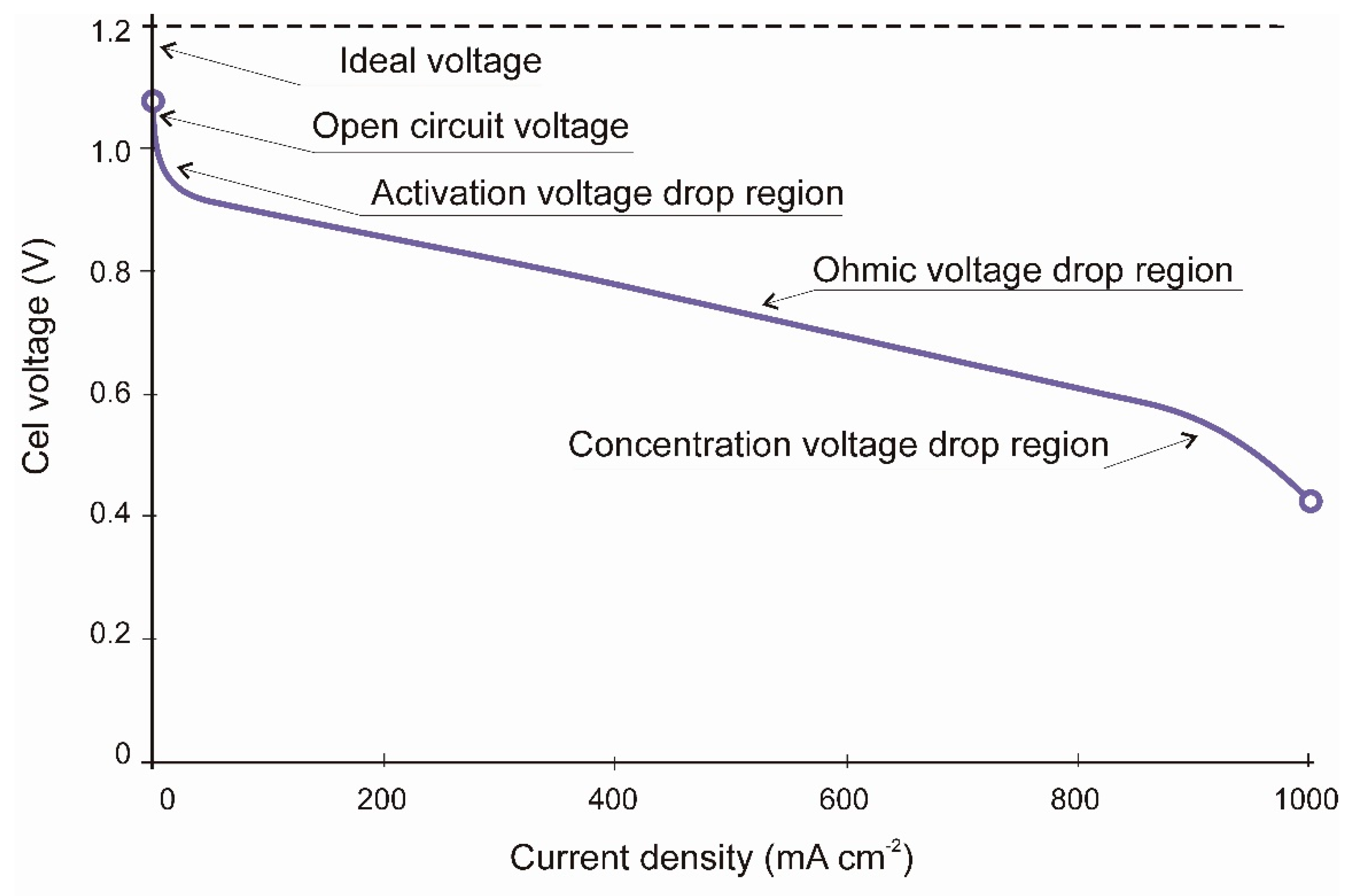
Figure 1 shows a typical cell polarization curve, which represents the main cell characteristics. As the current increases the voltage drops in three visible sections: the first voltage drop represents cell activation losses; the second section represents voltage losses by internal resistance, and the third section represents the voltage drop by gas transportation or concentration losses [
3].
In [
4] a model based on neural networks and used the Levenberg-Marquardt BP algorithm to identify the polarization curve characteristics is proposed. The model inputs were the airflow and the temperature, and the outputs signals were the current and voltage. The model presents good accuracy, however, the system demands training with high computational cost, and the authors suggested as an alternative the use of other optimization algorithms (OAs).
The identification of equations based in the model [
5] and using an OA is a clear tendency; these models have electrical and thermodynamic equations with around seven coefficients which allow tuning the model. The coefficients are identified using an optimization function which minimizes the error between simulated and real signals. In [
6] the current demand is used as input to generate de polarization curve. The identification of the coefficients was performed with an OA called hybrid genetic algorithm (HGA) that avoids the premature convergence of the simple genetic algorithm (SGA). The HGA needs to be fed with parameters close to previously identified ideal values. In [
7] a similar model to the previous one was used to identify the system with a particle swarm optimization (PSO) algorithm as an example of an algorithm which accepts initial parameters located in a very broad range. In [
8] a grouping-based global harmony search algorithm (GGHS) is presented to overcome the limits of the harmony search algorithm (HS). This work compared the GGHS with versions of HG and PSO, and concluded that the GGHS surpasses the mentioned algorithms. The grasshopper optimization algorithm (GOA) was proposed by [
9] to identify the parameters of three different PEMFCs, although GGHS and GOA require that the initial parameters fall within closer bounds. In [
10] the effective informed adaptive particle swarm optimization (EIA-PSO) as a modification of PSO that makes the algorithm configuration be dynamic to avoid finding fake solutions is proposed. However, this modification increases the computational cost in regards to a PSO. To overcome the mentioned problems of PSO, in [
11] a grey wolf optimizer is proposed, and this algorithm was tested with the classical model and five real different PEMFCs. Related to differential evolution (DE) algorithm framework, some authors have proposed variations to improve the performance of the scaling factor F. In [
12] the hybrid adaptive differential evolution algorithm (HADE) was proposed and compared with a PSO and two versions of differential evolutionary algorithms. The HADE surpasses the performance of the other OAs in terms of minimization speed. The comparison was made using test functions, but the PEMFC model and its optimization function was only carried out with HADE. Transferred adaptive DE (TRADE) is an improved DE algorithm applied to a PEMFC and SOFC models proposed by [
13]. Though, GGHS and GOA require that the initial parameters fall within closer bounds both presents attractive results. In a similar way, [
14] proposed a hybridization between a teaching learning-based optimization method (TLBO) and the DE algorithm; this application obtains better results with low computational cost, compared with single TLBO and DE separately. In [
15] the quantum-based optimization method (QBOM) applied to the identification of three voltage drop coefficients of a Nexa 1.2 kW PEMFC model is introduced. QBOM showed good accuracy and high minimization velocity in the identification. However it was applied in the identification of three parameters versus the seven parameters identified by previously mentioned works.
The above authors demonstrated the usefulness of OAs to parameter identification of PEMFC polarization curves. Moreover, the PEMFC polarization curve only represents the cell operation at one single stack temperature value and a single stable pressure of inlet gases.
The second main classification are the dynamic PEMFC models. Those models represent better the real behavior of a PEMFC because they show changes in the cell response when there are changes on the load current and other variables and consider the cell as a multiple-input multiple-output (MIMO) system. Each identification technique uses particular excitation inputs (such as steps, ramps or waves) and each one uses the outputs to build or to adjust transfer functions or state space models which include the fuel cell parameters. To facilitate the model identification, some PEMFC models can also be simplified by working with constant temperatures or by using linearization techniques.
A dynamic model used to test several control strategies was presented in [
16]. This model included inputs such as: inlet molar flow rates of oxygen and hydrogen; inlet temperatures of anode and cathode gas; and inlet coolant flow rate. After the excitation with input steps, the authors developed an empirical identification by monitoring the average power density and the average solid temperature. In [
17] the authors used transfer functions to model a PEMFC. This work used the stack current and the cathode oxygen flow rate as inputs and the stack voltage and the cathode total pressure as outputs. The model is able to predict the output signals near to the operation point. In [
18], a PEMFC Hammerstein model is presented. The inputs were current, stoichiometric oxygen, and cooling water flow, and the outputs were the partial pressure of O
2 and the stack temperature. The identification process used different random steps signals as inputs. In [
19] a PEMFC dynamic model that included the polarization curve characteristics and a double layer charge effect is proposed. The model input was a typical current demand of a DC-DC or a DC-AC. In [
20] a NARMAX model to represent the MIMO relations and to identify the coefficients satisfying the PEMFC voltage simulation is used. Also a NARMAX model is used by [
21] to represent a PEMFC and used a GA to the model identification, however, the model only represents the fuel cell temperature. Buchlozt and Krebs [
22] splits the PEMFC model into a dynamic part and a static part. The static model was identified with neural networks whereas the dynamic model was developed with a mix of transfer functions and linear state-space models. The model inputs were: current density, oxygen stoichiometry, gas supply pressure, and gasses relative humidity; other values as stoichiometry of oxygen and stack temperature were set to constant. The model output was the sum of the dynamic and the static voltage. The authors exposed that the split model allows to reduce the computational time and to improve the accuracy. A split model was also presented in [
23]. Regarding the dynamic part, the inputs were the current and the cathode pressure. All these works get deeper in the different relationships between input and output signals, so they model cell voltage responses to gas pressures and current variations. Nevertheless, PEMFC operation produces heat that changes the cell temperature. The temperature affects the cell performance and features as open circuit voltage, internal gas pressures, gas humidity, and internal resistances. Therefore, the use of temperature as an input variable will give more accuracy to the model despite the fact that the complexity and nonlinearity are increased.
Wang et al. [
24] developed a dynamic equation model where the temperature is considered to work in a closed loop. The model includes the electrochemical and thermal responses and the cell double layer charge effect, and has a good response in steady state and transients. The model characteristics are applicable in fault diagnosis and condition monitoring tasks; thus, this work was developed for a 500 W PEMFC and is not directly usable for other devices.
One recent approach [
25] used an equivalent electrical circuit model to represent a Nexa Ballard 1.2 kW PEMFC. This model simulated both the output voltage and the stack temperature. The model included fourteen electric coefficients and six thermal coefficients. They were identified with an evolution strategy (ES) algorithm. This work showed a model that includes the stack thermal dynamics and they applied GA to the parameter identification, however, the thermal model includes a piecewise heuristic function to link the temperature with the current to adjust the operation of the cooling system of the real cell. This last component and the model based on electrical circuits do not let one access the internal signal system. Salim et al. [
26] used an equations-based model which includes the thermal behavior of a Nexa 1.2 kW PEMFC. The voltage model was developed by fitting a polynomial curve which involves the classical voltage losses. The thermal model was developed using the sensible heat and latent heat. The identification process applies PSO with one independent optimization function for the voltage part and another for the thermal model. The results show high simulation accuracy. However, the model does not take into account the temperature in a closed loop, nor the cooling system performance of the device.
The present work is involved in a wider study related with fault diagnosis and condition monitoring of a Nexa Ballard 1.2 kW PEMFC installed in the Laboratory of Distributed Energy Resources [
27].
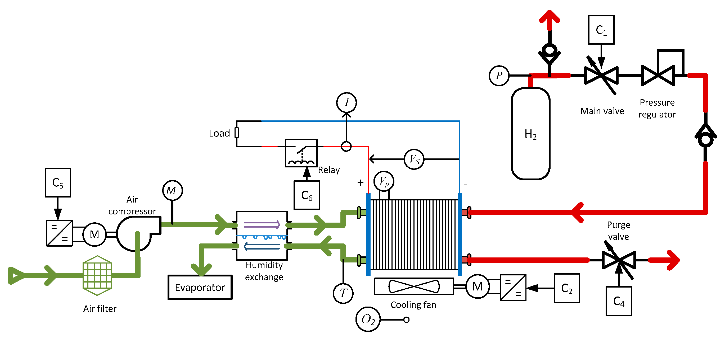
Figure 2 shows the block diagram of the complete Nexa system. Hydrogen is supplied from a compressed tank at adequate pressure. Reaction air is supplied by means of a compressor and measured by a mass flow meter. Temperature is measured at the air outlet, so this is the stack temperature. The system is cooled by a fan in order to maintain the temperature under the upper limit. Voltage of the complete stack and the last two cells is measured in order to determine when the hydrogen purge valve is opened to eliminate accumulated impurities. Current generated by the fuel cell is measured for two reasons: to open the relay if current exceeds the maximum and to act over the air compressor to maintain the correct stoichiometric relationship.
Table 1 shows the manufacturer values of the PEMFC.
The overall study requires a model able to represent the device and that uses the maximum amount of measured data. In addition, the identification process must be accurate, fast, and with the lowest computational cost as possible to make the model suitable to be used in real time applications. This paper uses the model presented by [
24] to fit the Nexa 1.2 kW PEMFC real data. Moreover, several GAs are used and they are compared in order to look for the best strategy to fit the model.
Section 2 shows the description of the model.
Section 3 shows the adjustment of the equations coefficients to fit the PEMFC Nexa behavior. The results of the identification and the model validation are presented in
Section 4. Finally, we present some conclusions and future work suggestions.
2. The PEMFC Model
The model presented in this paper is an extension of the dynamic model presented in [
24] where the model is explained in detail. The model assumes the following conditions to simplify it: (a) One-dimensional treatment, (b) Ideal and uniformly distributed gases. (c) Constant pressures in the flow channels. (d) Fuel and oxidant are humidified. So, the effective anode water vapor pressure is 50% of the saturated vapor pressure while the effective cathode water pressure is 100%. (e) The fuel cell works under 100 C and the reaction product is a liquid phase. (f) Thermodynamic properties are evaluated at the average stack temperature, and the overall specific heat capacity of the stack is assumed to be a constant. (g) Parameters for individual cells can be lumped together to represent a fuel-cell stack.
Equations represent several phenomena as: (a) gas diffusion in the electrodes, (b) material conservation, (c) fuel cell output voltage, starting from the Nernst equation and including the voltage drop by activation, internal resistances, and concentration, (d) double-layer charging effects present in the fuel cell membrane, and (e) thermodynamic energy balance.
This work only presents the key equations and the modifications included. Data used for fitting the model was obtained from the Nexa 1.2 kW PEMFC software (NexaMon OEM 2.0) which gives information about the key variables as well as inlet pressures and cooling system variables that must be taken into account to model the thermal performance of the fuel cell.
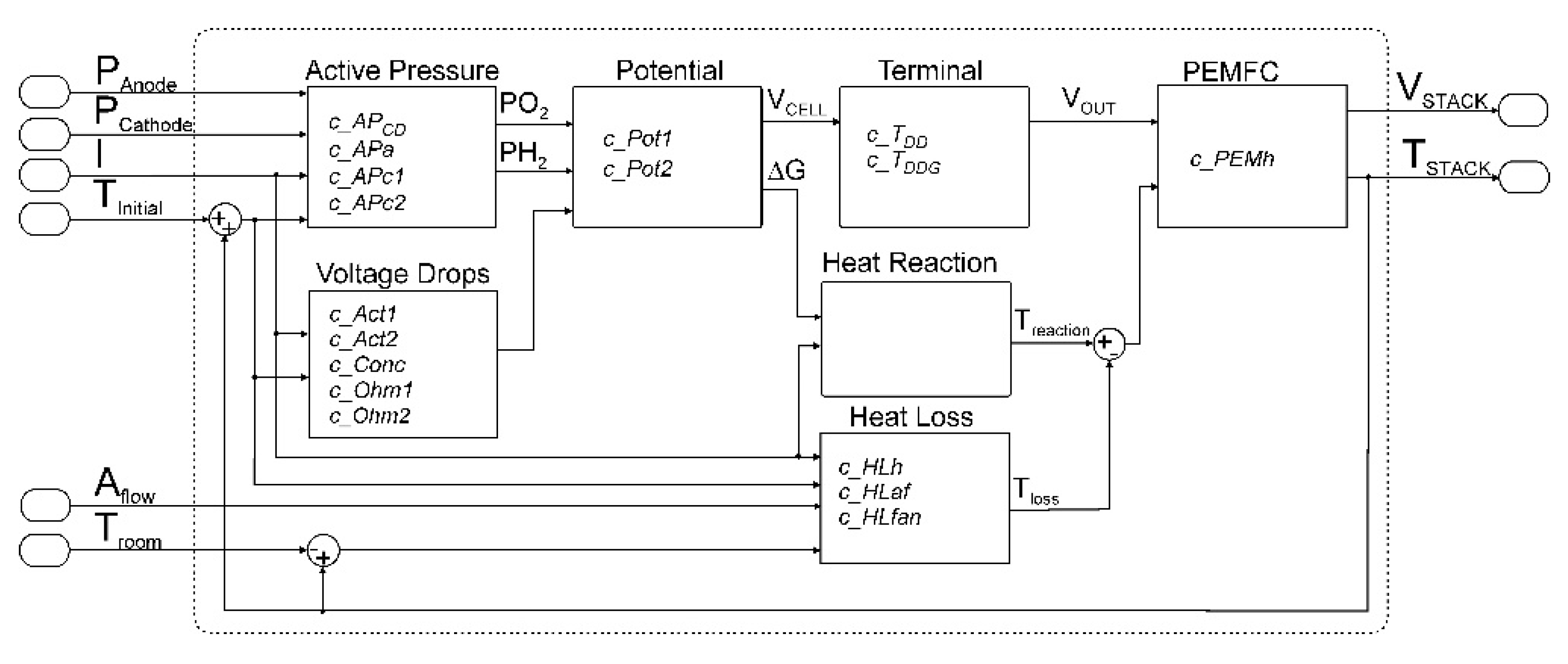
Figure 3 shows the PEMFC model, including the input/output signals.
The model was implemented under a LabVIEW
® (2010, National Instruments, Austin, TX, USA) environment. The equations were grouped into electrical and thermal sets. The most remarkable equation in the electrical set is the cell potential E
cell(t) which is calculated with the Nernst’s equation. Equation (1) is a simplification of the Nernst’s due the assumptions mentioned above. E
d,cell(t) represents the electrical effect of gas pressure changes during load transients and classical voltage drops:
where T(t) is the cell temperature (K); F is the Faraday constant (96487 coulombs/mol); R is the ideal gas constant (8.3143 J/mol K); E
0(t) is the reference potential at standard conditions (298 K, 1 atm); p
H2*(t) is the H
2 effective partial pressure; p
O2*(t) is the O
2 partial pressure. E
d,cell(t) is initially modelled in Laplace domain as Equation (2) and implemented in the time domain in Equation (3):
where
I(
t) is the current (A);
p is the simulation step;
d,
τ are a delay constants related to PEMFC distribution layers.
Regarding the thermal equations set, the thermal loss equation was modified to include the cooling system of Nexa PEMFC. It is identified in Equation (4):
where,
hcell is the convective heat transfer coefficient (W/m
2·K) of the stack;
Ncell is the number of cells in the stack;
Acell is the cell area (cm
2). The control system of a Nexa includes the operation of a fan and cooling system, providing oxygen inlet and keeping the temperature under a limit to keep operation conditions and avoid membrane damage.
Af(
t) is a coefficient to adjust the temperature related to the cooling system.
The proposed model has been split into functional blocks (
Figure 3), so each block can be analyzed separately for fault diagnosis purposes. Each block contains tunable coefficients to reduce the difference between the real and the simulated signals. The blocks and its respective coefficients are described below. The active pressure block calculates the effective partial pressure in the anode and the cathode side. The block has four parameters:
c_APCD is a parameter related to the cell current density.
c_APa is a parameter related to the distance between the anode channel and the catalyst surface.
c_Apc1 is a parameter related to the distance between the cathode channel and the catalyst surface.
c_Apc2 is a parameter that fits the pressure of saturated H2O curve in function of the temperature.
The voltage drop block represents the voltage losses by activation, internal resistance, and concentration. The coefficients are:
c_Act1 is a parameter related to the activation voltage drop that only depends on temperature.
c_Act2 is a parameter related to the activation voltage drop, that depends on current and temperature.
c_Ohm1 is the parameter related to ohmic losses that depends on current and temperature.
c_Ohm2 is a parameter related to ohmic losses that only depends on cur-rent.
c_Conc is a parameter related to the voltage concentration drop.
The potential of the cell are calculated in the potential block which includes two coefficients:
The terminal block represents the electrical global stack behavior. This block includes the cell potential, the voltage losses, and a voltage drop by fuel and oxidant delays during load transients. The terminal block has the following parameters:
The heat loss block represents thermal losses that leave the stack by air convection and energy absorbed by exhaust gases. The parameters are:
c_HLh is a gain that affect the overall heat loss.
c_HLaf is the parameter fitting the thermal loss associated to the cathode side. It is included in the stack thermal loss.
c_HLfan is a gain associated with the cooling fan system and it is included in the stack thermal loss.
The PEM block merges the electrical and the thermal equations to represent the global PEMFC performance. This block has one parameter:
A complete set of parameters (PS) can be used to simulate the PEMFC. Therefore, the goal of this research will be the search for the set of parameters that minimizes the difference between the PEMFC real outputs and the model outputs. The notation used to define the different elements of the algorithms is presented below:
A population of parameter sets (an array of parameter sets) will be denoted as:
where PS
k is the population of the k-th iteration:
where PS
jk is j
th parameter set of the kth population and the i
th model parameter will be noted as c
ki,j. For example, c
71,2 corresponds with the value of parameter 1 c_APCD in parameter set 2 of the 7th population.
The model was programmed and tested with initial coefficients taken from [
24] and from the device manufacturer manuals. This PEMFC model was simulated using real inputs signals obtained from real operation of a Nexa 1.2 kW PEMFC using the device software (NexaMon OEM 2.0).
Figure 4 shows the predicted voltage and temperature as well as the real values. Therefore, despite the fact that there is a significant difference, the model seems to be suitable to represent the system dynamics after a suitable parameter fitting. The MSE obtained with the initial coefficients represent a challenge in the identification process because the huge initial errors make it difficult to find the optimal parameter set.
3. Parameter Identification
The PEMFC model, the identification process, and the algorithms were implemented in the LabVIEW
® environment, achieving a modular and versatile programming structure.
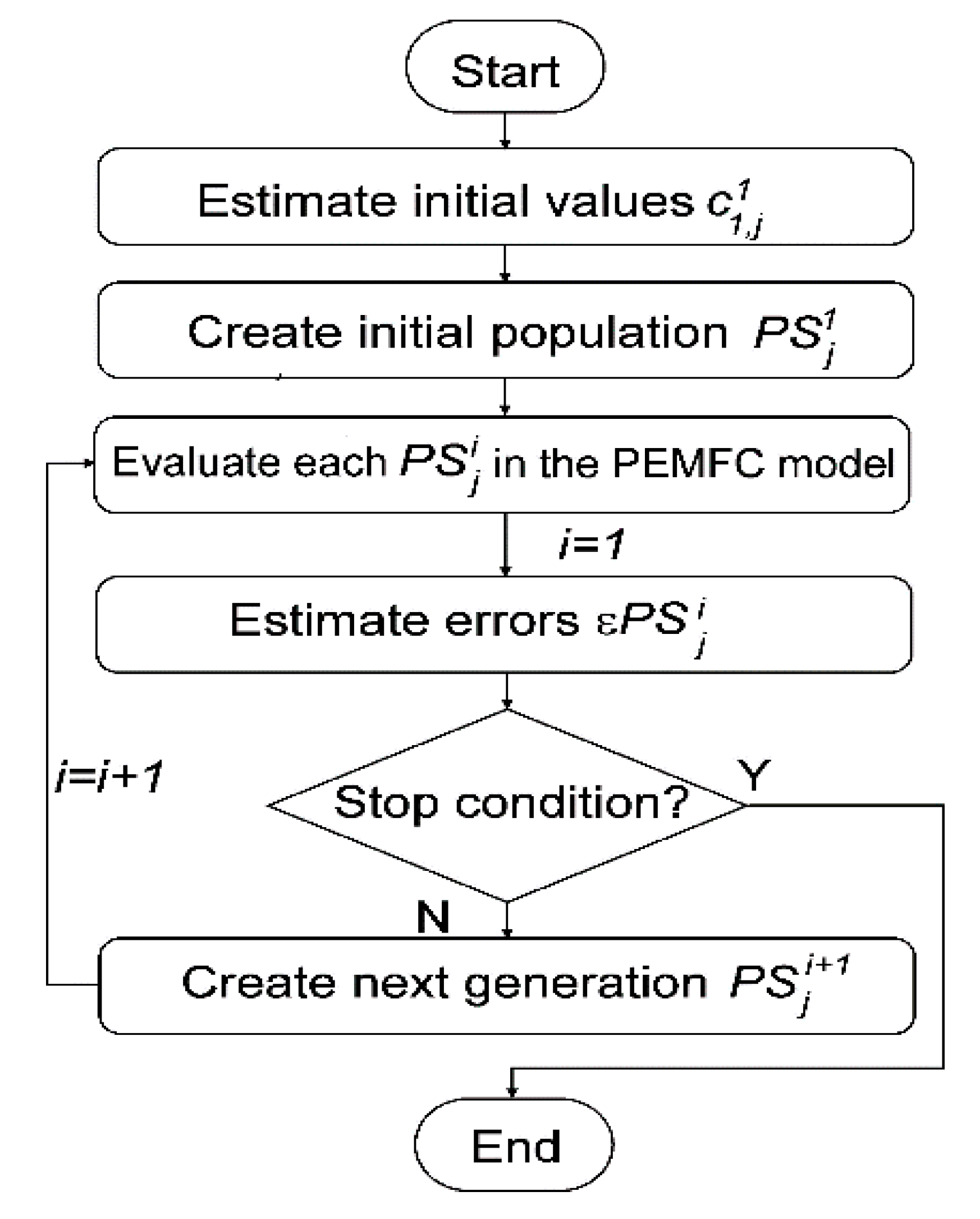
Figure 5 shows the identification process. The process begins with the estimation of the initial coefficients. The second step is the creation of a first population using a random function starting from the initial coefficients set. In the third step, each coefficient set is simulated in the model with a real data input file. At least, outputs from simulated and real data are compared in order to calculate the error. The optimization process ends when a stop condition is met. The stop condition can be specified as a threshold on the error or as a maximum number of iterations. If the stop condition is not fulfilled, the OA creates a new population by using a genetic algorithm. This new population is evaluated again in Step 3, thus repeating the process until the optimization ends.
The initial population is created from an initial
PS11 as indicated in Equation (5):
where
z is a random number in the range [−1, 1] and
vd is a value to generate initial dispersion (some GAs include special criteria to create this first population). Each
is simulated and comparing the real output with simulated outputs, to calculate the error
with Equation (6):
where
εV is the output voltage error, and
εT is the stack temperature error, they are calculated as:
where
RMSEV and
RMSET stand for the root mean square error between real and simulated output voltage signals and stack temperature signals, respectively. FSV and FST stand for the device full scales related to the output voltage signal and stack temperature signal, respectively:
where
n is the data length;
OutR(
t) and
OutS(
t) are the real and simulated output signal values at time
t, respectively. Therefore, the goal is to minimize
.
Each OA uses a particular policy to create the new population from the previous evaluated population. The goal is to converge to the optimal solution in the minimum number of steps. In order to perform this operation, OAs include random components to search for the global best solution which include values of dispersion to spread or to focus the offspring near a possible solution for each iteration.
Previous works dealing with PEMFC parameters identification have tested PSO [
7,
26], HADE [
12] and EA [
25]. HADE is an evolution in parameter identification that surpasses the PSO results and EA was tested to identify the thermal component of a PMFC. This paper tests the previous three algorithms and includes two new proposals to solve some difficulties found in the model identification.
One important feature of PSO is its ability to gradually focus the search around the minimum. However, if the algorithm falls around a local minimum, PSO losses the ability to find other possible solutions with better results. This paper proposes the introduction of periodic perturbations inside the population in order to force PSO reactivation. The perturbation will consist of a new population
based on the best global solution:
where
CiGBest is de
i coefficient belonging to the global best solution until iteration
k − 1,
z is a random number in the range [−1; 1], and n is a perturbation value. This proposal is named PSOp because the use of perturbations.
The PEMFC model identification uses seventeen parameters that must be evaluated so the process has a considerable computational demand. Therefore, in order to simplify the identification process, another GA called scout genetic algorithm (ScGA) is proposed. RGA is a minimalistic GA that creates new populations based on the overall best solution found. The progeny is split into two groups, the offspring and the scouts:
where
j is the population size and
Sn is a value in the range [0; 1] which represents the percent of scouts in the population. The offspring population is calculated as:
where
PSjGBest is the coefficient set achieving the best solution until iteration
k,
zj is a random number in the range [−1; 1] which modifies all values in one set, and
vos is the spread value of offspring which modifies the whole coefficient set.
The scout population is:
where each
is calculated as:
where
ciGBest is the coefficient
i of the global best solution until iteration
k.
zi is a random number in the range [−1; 1] which affects only the
ith coefficient, and
vSc is the spread scout value.
4. Results
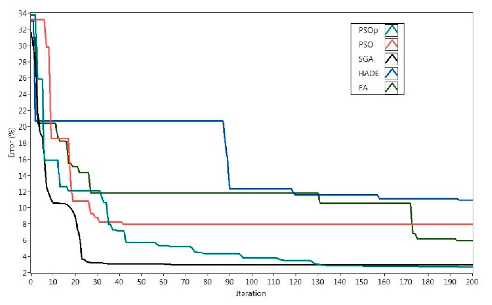
The identification process was carried out with the five OAs explained in the previous section: PSO, HADE and EA as in previous approaches; PSOp and ScGA as the proposed new approaches. For all OAs, the population size (j) was set to 100 individuals starting from the same initial PS1. The initial population dispersion (vd) was set to 0.5 to create enough diversity. The maximum iteration number (k) was set to 200 in order to give the same opportunity to each OA.
Figure 6 shows the global best error reached by each OA. The figure shows fast responses for all the algorithms. However, HADE, EA, and PSO became stuck early in high errors. PSOp and ScGA produced the lowest errors.
Table 2 shows that ScGA is the best option to identify the PEMFC model regarding the precision, velocity and computational cost. In the second place, the PSOp is the most accurate algorithm, but its computational cost and velocity are not the best. The EA shows middle-level of precision and good computational time that places it in the third position. PSO presents the known phenomena of getting stuck around fake local minimal. Finally, HADE is placed in the last position. The optimization velocity of HADE, EA, and PSOp algorithms indicates that an increment in the number of iterations could give better results if the simulation time of the parameter identification process is minimal.
Table 3 shows the found values in the identification process, these values were used to validate the identified model.
Due to the model complexity and its non-linearity, the set of identified values create one of the multiple possible solutions that belong to a Pareto front. To validate the specific solution, the model was configured with the identified parameters and tested against two load profiles obtained from saved data files from a Nexa PEMFC.
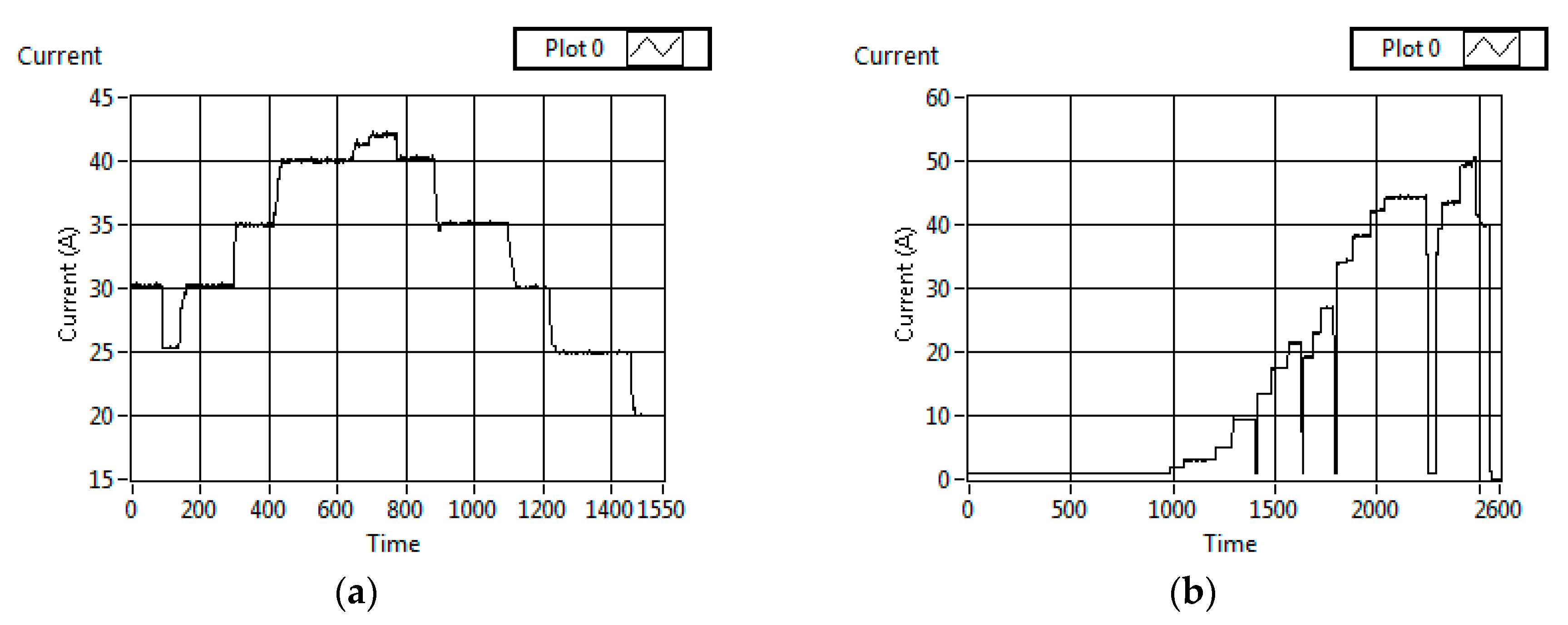
Figure 7 shows the current load profiles, which force different dynamical PEMFC behaviors. The current profiles are loaded in the model with the other input signals.
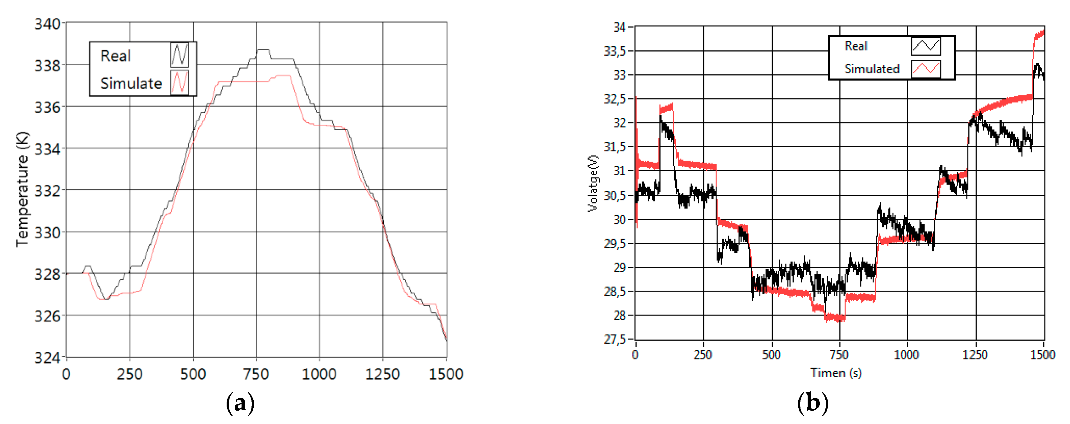
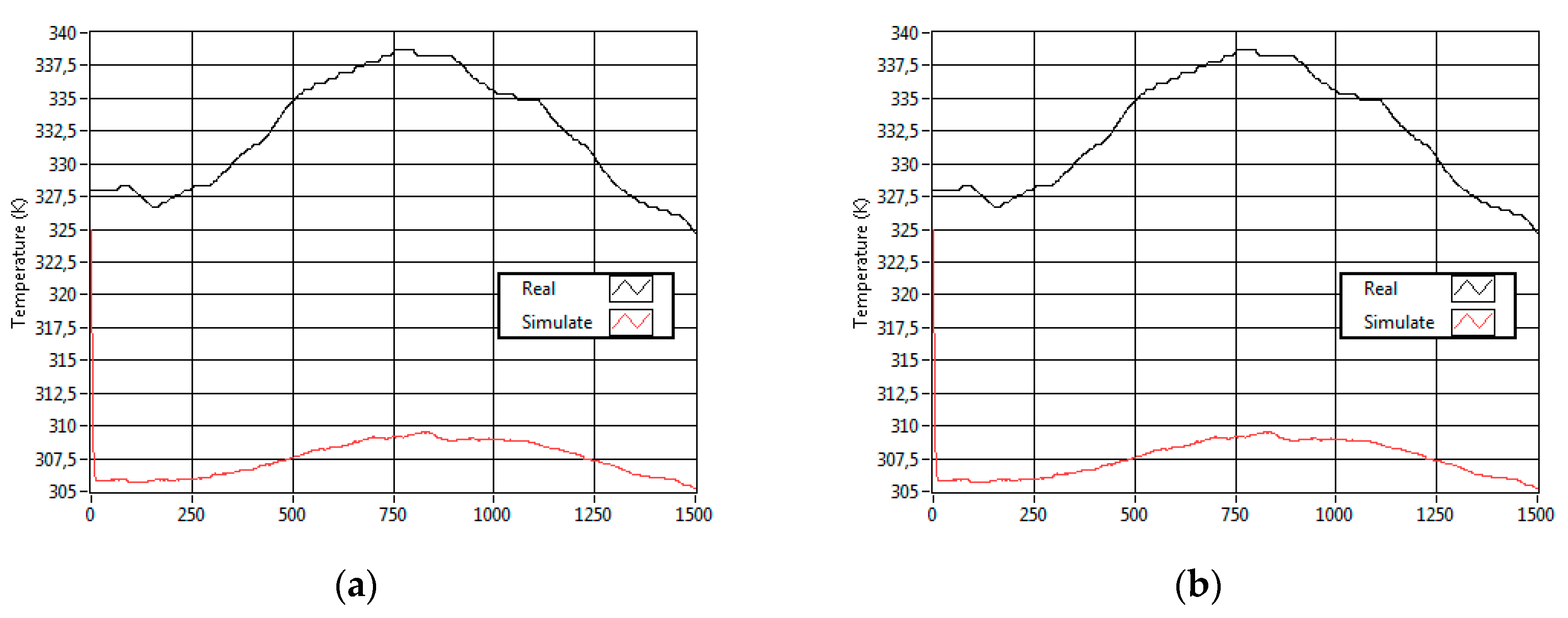
Figure 8 shows the model validation performed with the current profile 1. In the stack temperature graphic (left) the simulated plot is ahead, but closely following the real plot. The output voltage graphic shows that the simulated voltage follows the real data, but has a slow response respect to the changes of load.
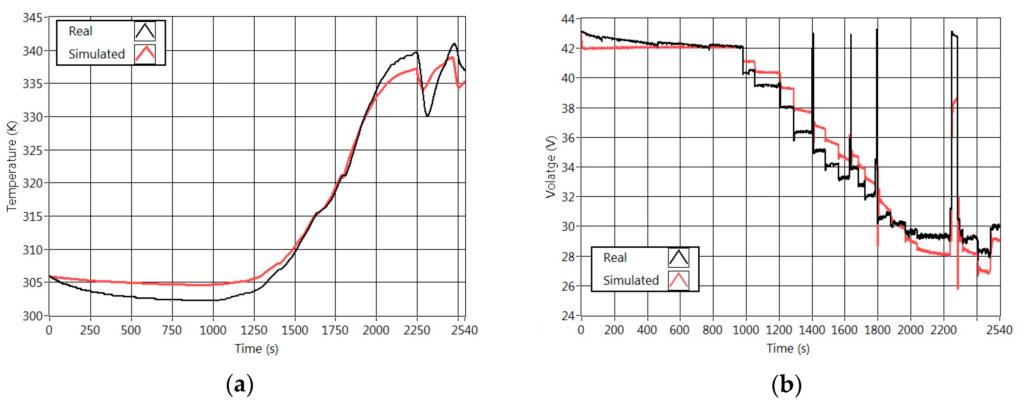
Figure 9 shows the Profile 2 validation. Both graphics confirm the behavior mentioned above. However, it is remarkable that the temperature simulated cannot decrease in the first section of the profile.
Table 4 shows the errors in the signals of voltage, temperature and the mean of voltage -temperature using Equations (7) and (8), respectively.
5. Conclusions and Future Works
This paper presents a non-linear model able to represent the real performance of a PEMFC, which includes not only the electrical behavior but also the thermal behavior. The model has been fit to represent a real Nexa 1.2 kW PEMFC behavior with the aid of GA. The initial coefficients extracted from other papers produced an initial error above 30%.
This fact created an interesting challenge because the literature about PEMFC parameter fitting identification processes starts with values close to the expected target. This research compares five different GA algorithms to explore the best approach. Three of this GAs were taken from the literature and two more were proposed in this work. It is shown that the proposed PSOp and ScGA are remarkable algorithms because of their good precision and low computational cost.
The identified model was tested with real data and it showed good results with overall errors under 3%. Despite the fact that the identification process achieves low errors, accuracy improvement of the model will always be needed. Therefore, the work related to the model precision must continue focused on analyzing the dynamic model behavior.
The PEMFC block model is behaving as a grey box model because some internal signals are accessible. It is a useful feature to apply condition monitoring and fault diagnosis techniques. The use of the identified model for real PEMFC fault diagnosis and condition monitoring will be the next step of the research. The application of this complex and well fit mathematical model will improve the diagnosis power of the standard procedures. Due to the low computational cost of the identification process, the real device can be run parallel with the model. Therefore, the model can be fed with the same inputs as the system in order to perform condition monitoring and diagnosis tasks. The next challenges of this work are determination of the Pareto front of the possible solutions and the boundaries of each parameter under normal device operation conditions. Study of the parameter evolution using a chronological sequence of data files. Those identified values and its variations will be analyzed to find its relationship with PEMFC aging symptoms, and PEMFC faults.

 ,
, 


