Identification of the Heat Equation Parameters for Estimation of a Bare Overhead Conductor’s Temperature by the Differential Evolution Algorithm


Abstract
:1. Introduction
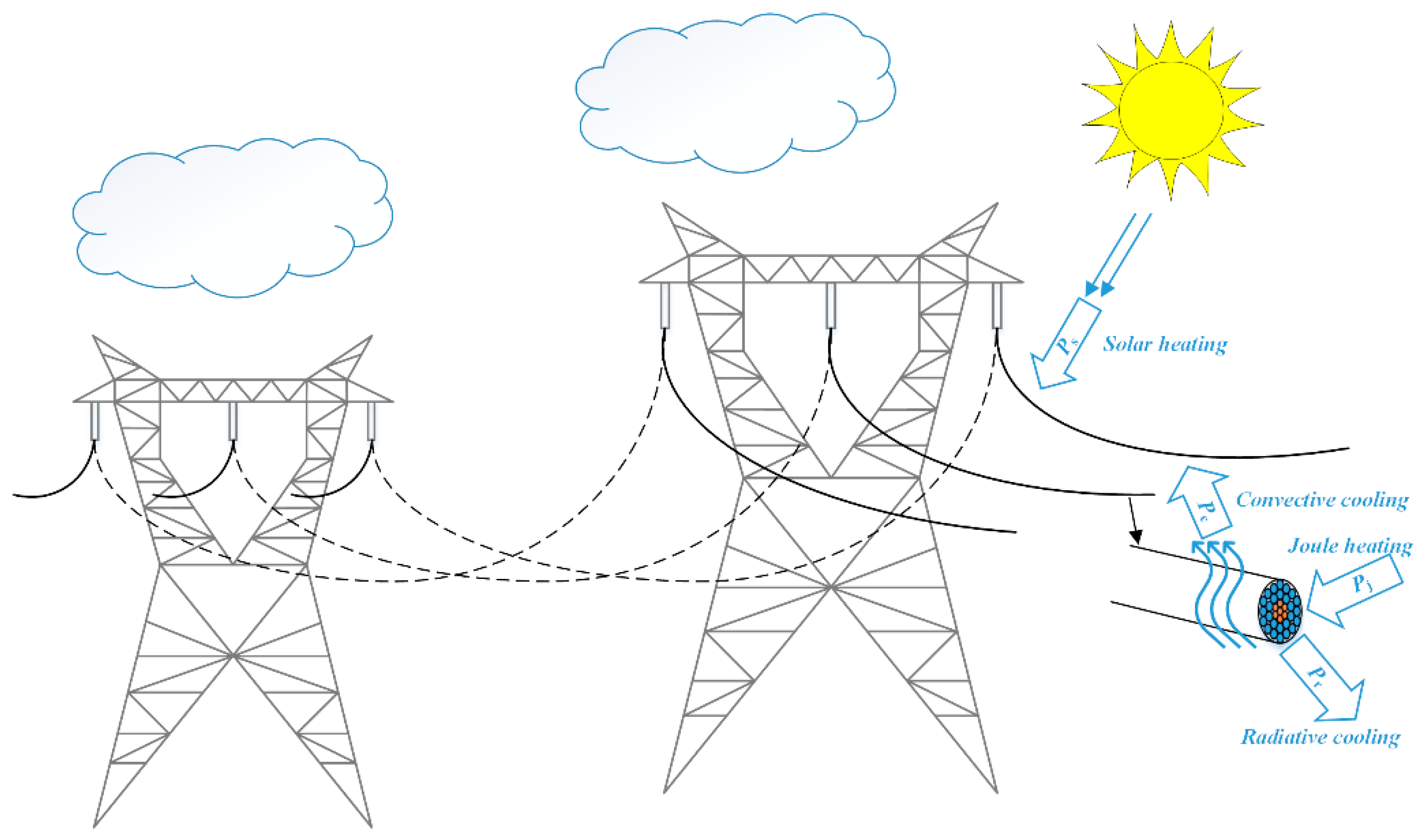
2. Conductor Dynamic Model
2.1. The Influence of the Joule Losses on the Conductor Temperature
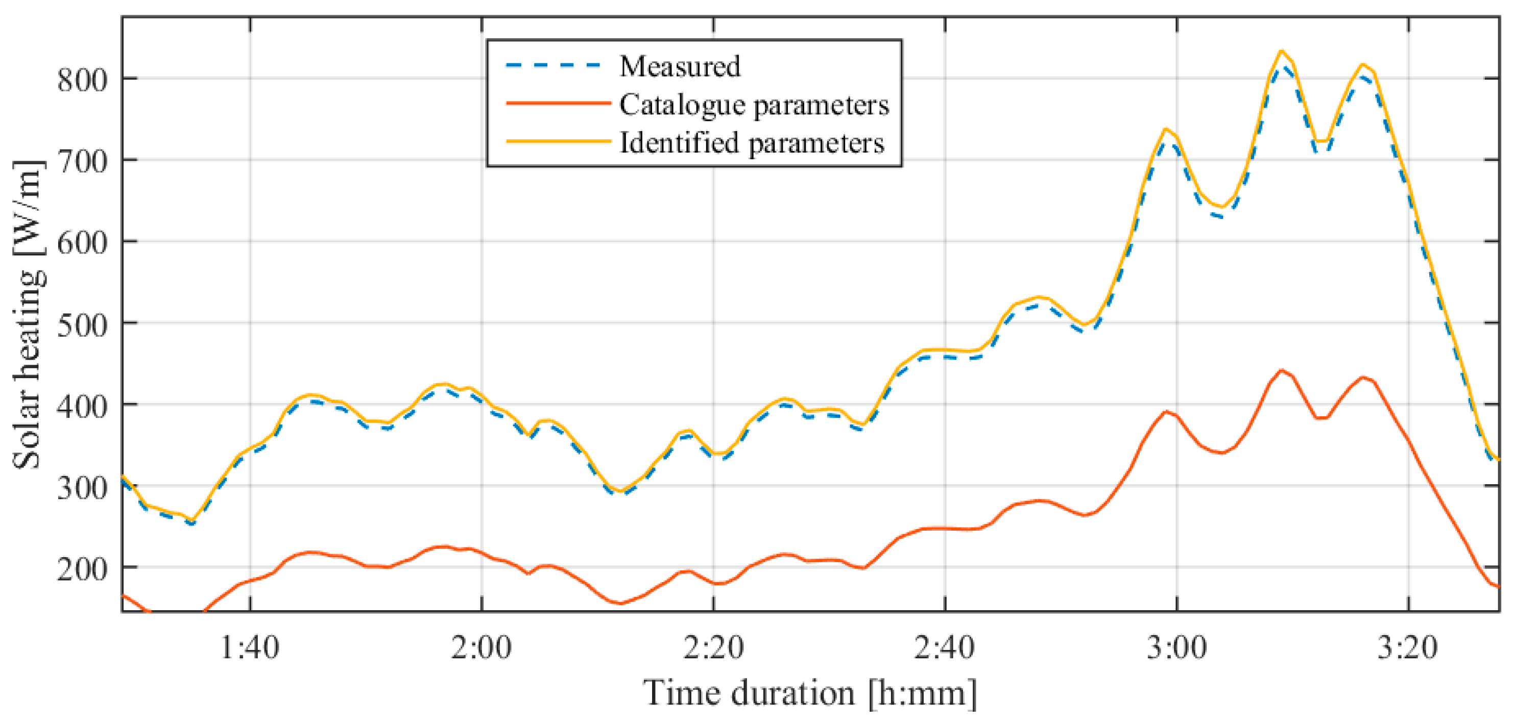
2.2. Solar Heating of the Conductor
2.3. Convective Cooling of the Inductor
2.4. Radiative Cooling of the Conductor
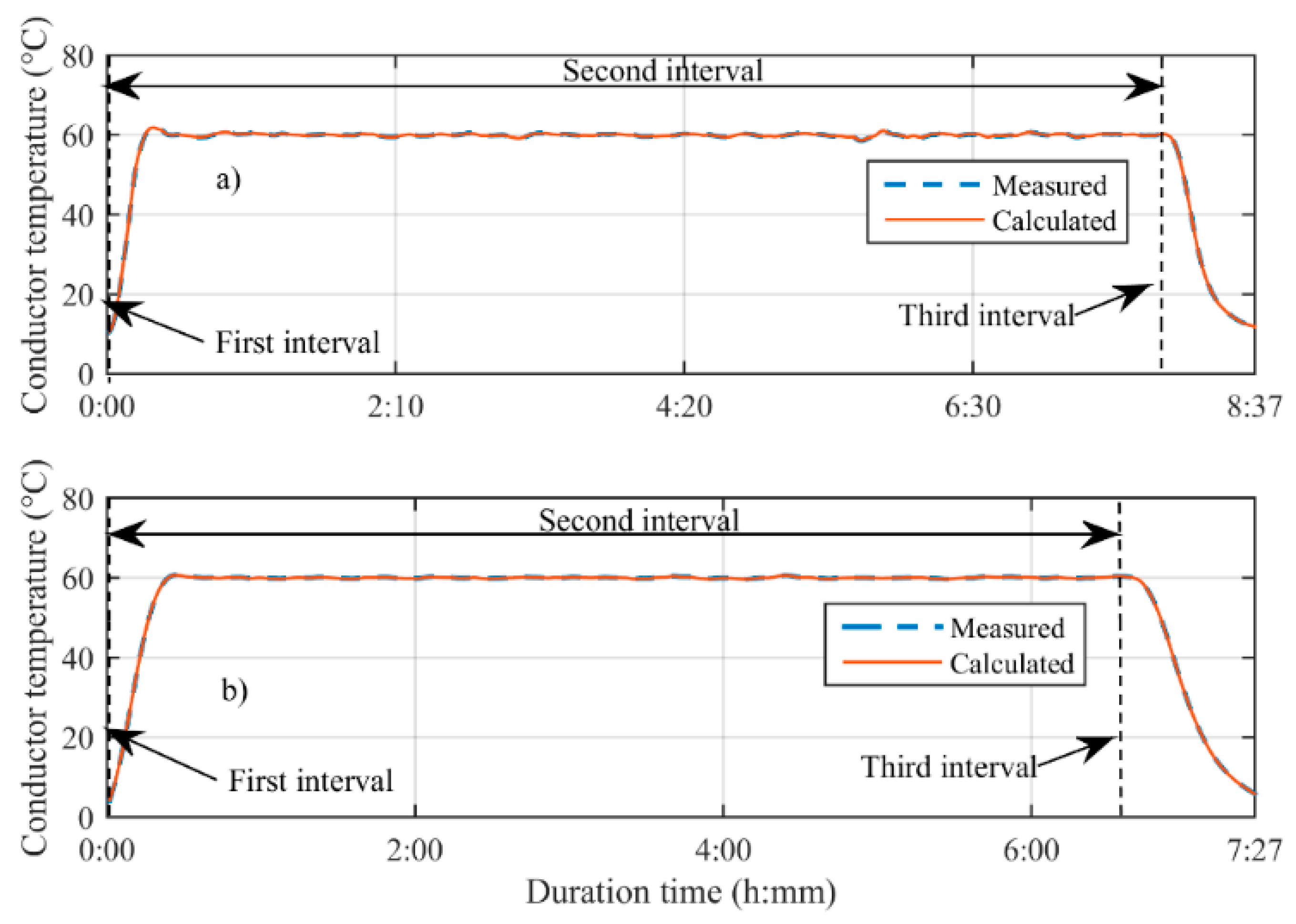
2.5. Calculation of the Conductor Temperature
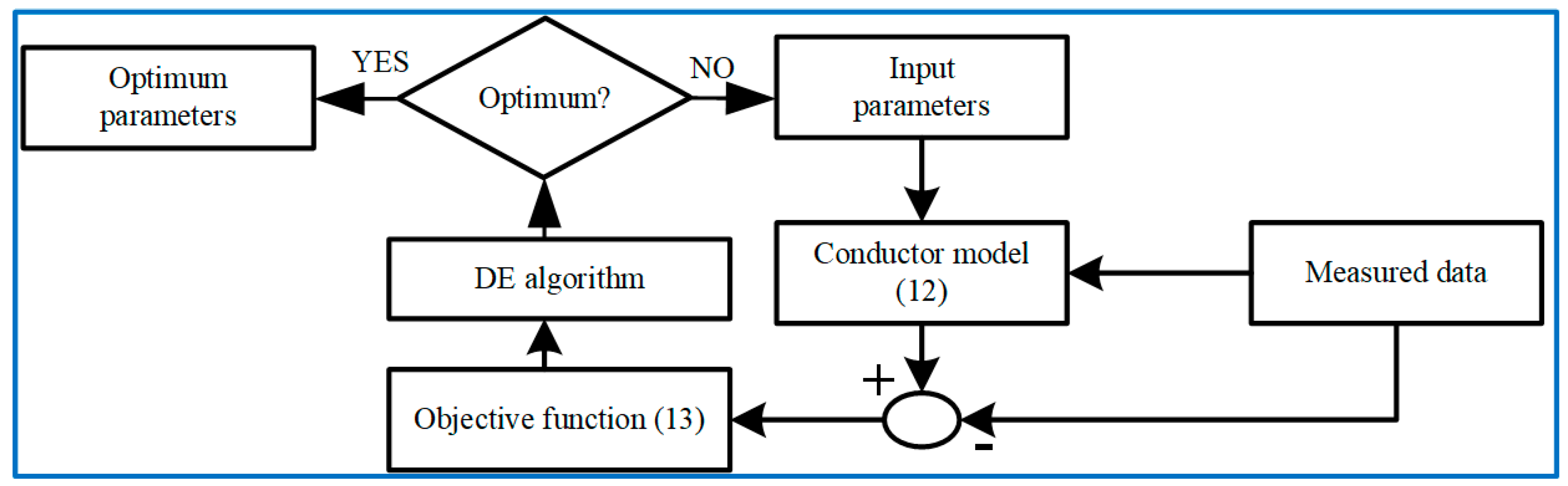
3. Determination of the Conductor Temperature Using DE
3.1. Differential Evolution
3.2. Determining Parameters
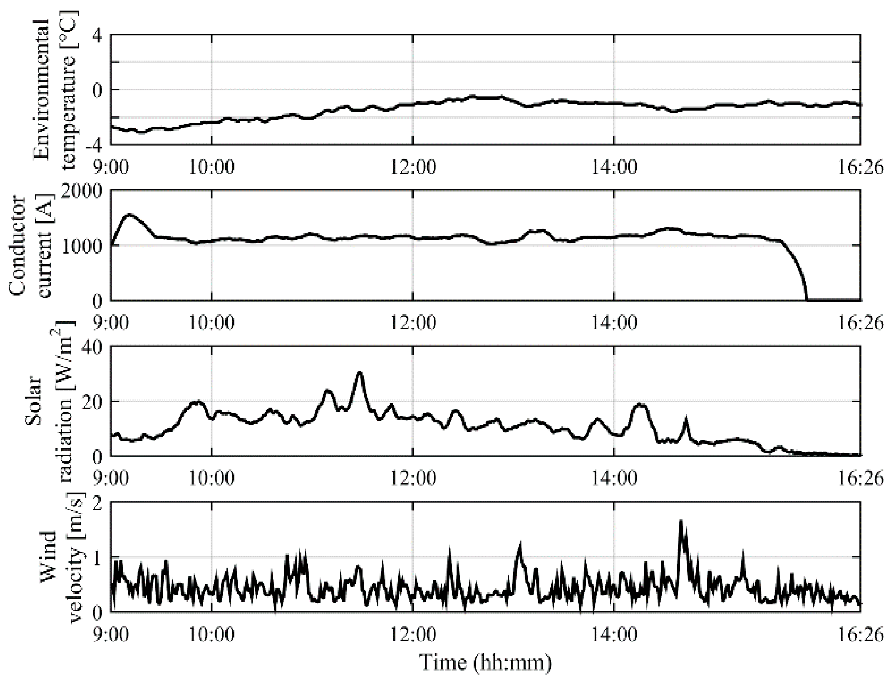
4. Experimental Set-Up and Measurements
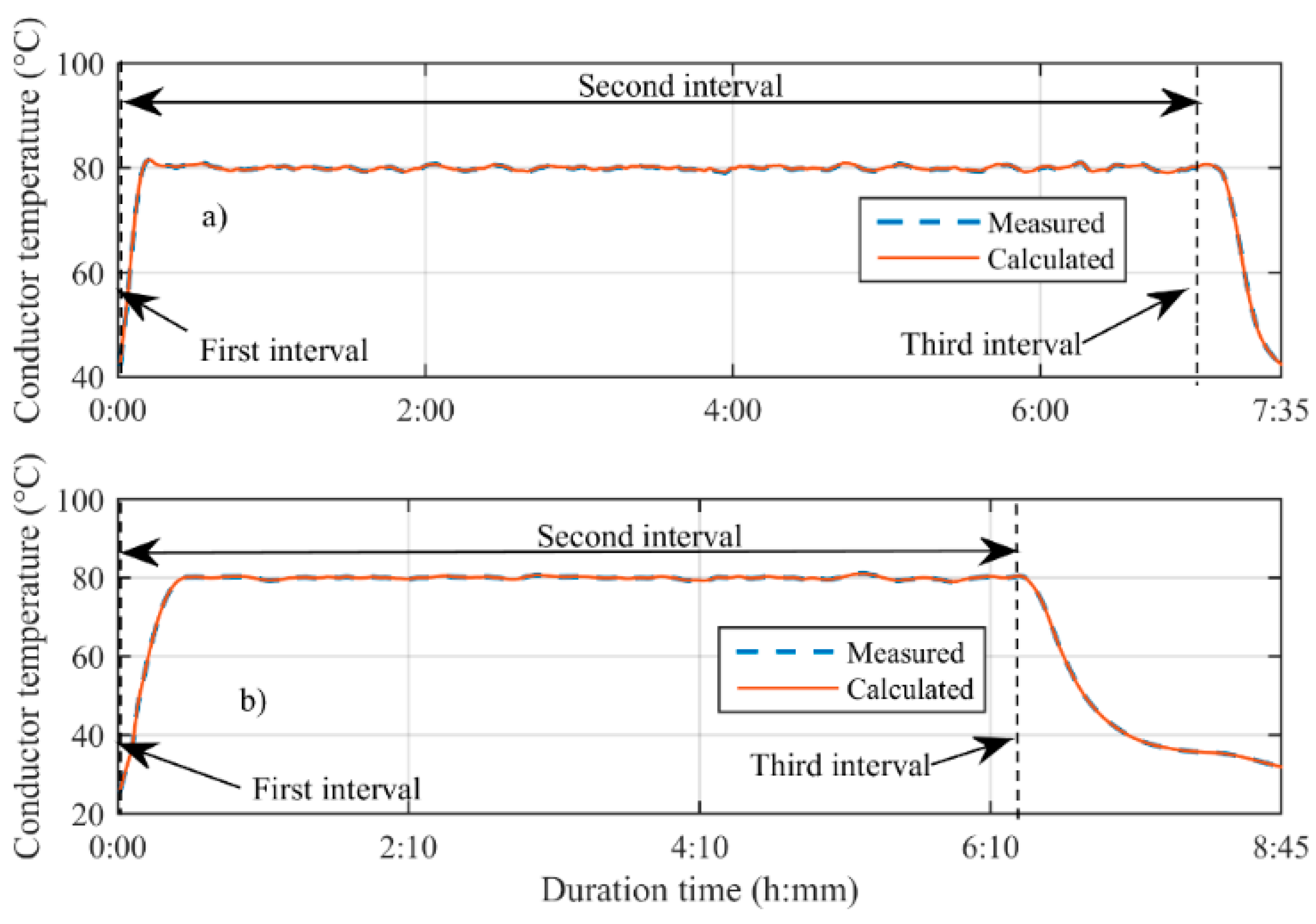
5. Results
6. Conclusions
Supplementary Materials
Author Contributions
Funding
Conflicts of Interest
References
- Muhr, M.; Pack, S.; Jaufer, S.; Haimbl, W.; Messner, A. Experiences with the Weather Parameter Method for the use in overhead line monitoring systems. Elektrotechnik und Informationstechnik 2008, 125, 444–447. [Google Scholar] [CrossRef]
- Gomez, F.A.; de Maria, J.M.G.; Puertas, D.G.; Baïri, A.; Arrabé, R.G. Numerical study of the thermal behaviour of bare overhead conductors in electrical power lines. In Recent Researches in Communications, Electrical & Computer Engineering; World Scientific and Engineering Academy and Society (WSEWAS): Montreux, Switzerland, 2011; pp. 149–153. [Google Scholar]
- Šnajdr, J.; Sedláček, J.; Vostracký, Z. Application of a line ampacity model and its use in transmission lines operations. J. Electr. Eng. 2014, 65, 221–227. [Google Scholar] [CrossRef]
- Wiecek, B.; De Mey, G.; Chatziathanasiou, V.; Papagiannakis, A.; Theodosoglou, I. Harmonic analysis of dynamic thermal problems in high voltage overhead transmission lines and buried cables. Int. J. Electr. Power Energy Syst. 2014, 58, 199–205. [Google Scholar] [CrossRef]
- Theodosoglou, I.; Chatziathanasiou, V.; Papagiannakis, A.; Więcek, B.; De Mey, G. Electrothermal analysis and temperature fluctuations’ prediction of overhead power lines. Int. J. Electr. Power Energy Syst. 2017, 87, 198–210. [Google Scholar] [CrossRef]
- Krontiris, T.; Wasserrab, A.; Balzer, G. Weather-based Loading of Overhead Lines—Consideration of Conductor’s Heat Capacity. In Proceedings of the International Symposium of Modern Electric Power Systems, Wroclaw, Poland, 20–22 September 2010; pp. 1–8. [Google Scholar]
- Jiang, J.A.; Liang, Y.T.; Chen, C.P.; Zheng, X.Y.; Chuang, C.L.; Wang, C.H. On Dispatching Line Ampacities of Power Grids Using Weather-Based Conductor Temperature Forecasts. IEEE Trans. Smart Grid 2018, 9, 406–415. [Google Scholar] [CrossRef]
- Pytlak, P.; Musilek, P.; Lozowski, E.; Toth, J. Modelling precipitation cooling of overhead conductors. Electr. Power Syst. Res. 2011, 81, 2147–2154. [Google Scholar] [CrossRef]
- Yang, Y.; Harley, R.G.; Divan, D.; Habetler, T.G. Overhead conductor thermal dynamics identification by using Echo State Networks. In Proceedings of the International Joint Conference on Neural Networks, Atlanta, GA, USA, 14–19 June 2009; pp. 3436–3443. [Google Scholar]
- Sidea, D.; Baran, I.; Leonida, T. Weather-based assessment of the overhead line conductors thermal state. In Proceedings of the IEEE Eindhoven PowerTech, Eindhoven, The Netherlands, 29 June–2 July 2015. [Google Scholar]
- Liu, J.; Yang, H.; Yu, S.; Wang, S.; Shang, Y.; Yang, F. Real-Time Transient Thermal Rating and the Calculation of Risk Level of Transmission Lines. Energies 2018, 11, 1233. [Google Scholar] [CrossRef]
- Wang, Y.; Mo, Y.; Wang, M.; Zhou, X.; Liang, L.; Zhang, P. Impact of Conductor Temperature Time–Space Variation on the Power System Operational State. Energies 2018, 11, 760. [Google Scholar] [CrossRef]
- CIGRE Working Group 22.12. The Thermal Behaviour of Overhead Conductors Section 1 and 2: Mathematical Model for Evaluation of Conductor Temperature in the Steady State and the Application Thereof. Electra 1992, 4, 107–125. Available online: https://e-cigre.org/publication/ELT_144_3-the-thermal-behaviour-of-overhead-conductors-sections-1-and-2 (accessed on 7 August 2018).
- IEEE. IEEE Std 738-2012: IEEE Standard for Calculating the Current-Temperature Relationship of Bare Overhead Conductors; IEEE Standard Association: Washington, DC, USA, 2013. [Google Scholar]
- CIGRE Working Group B2. 43. Guide for Thermal Rating Calculations of Overhead Lines; Technical Brochure 601; CIGRE: Paris, France, 2014; Available online: https://e-cigre.org/publication/601-guide-for-thermal-rating-calculations-of-overhead-lines (accessed on 7 August 2018).
- Schmidt, N.P. Comparison between IEEE and CIGRE ampacity standards. IEEE Trans. Power Deliv. 1999, 14, 1555–1559. [Google Scholar] [CrossRef]
- Arroyo, A.; Castro, P.; Martinez, R.; Manana, M.; Madrazo, A.; Lecuna, R.; Gonzalez, A. Comparison between IEEE and CIGRE Thermal Behaviour Standards and Measured Temperature on a 132-kV Overhead Power Line. Energies 2015, 8, 13660–13671. [Google Scholar] [CrossRef] [Green Version]
- Zhan, Q.; Wu, S.; Li, Q. A PSO identification algorithm for temperature adaptive adjustment system. In Proceedings of the IEEE International Conference on Industrial Engineering and Engineering Management (IEEM), Singapore, 6–9 December 2015. [Google Scholar]
- Meenal, R.; Selvakumar, A.I. Temperature based model for predicting global solar radiation using genetic algorithm [GA]. In Proceedings of the International Conference on Innovations in Electrical, Electronics, Instrumentation and Media Technology (ICEEIMT), Coimbatore, India, 3–4 February 2017. [Google Scholar]
- Marčič, T.; Štumberger, G.; Štumberger, B.; Hadžiselimović, M.; Virtič, P. Determining parameters of a line-start interior permanent magnet synchronous motor model by the differential evolution. IEEE Trans. Magn. 2008, 44, 4385–4388. [Google Scholar] [CrossRef]
- Glotic, A.; Pihler, J.; Ribic, J.; Stumberger, G. Determining a gas-discharge arrester model’s parameters by measurements and optimization. IEEE Trans. Power Deliv. 2010, 25, 747–754. [Google Scholar] [CrossRef]
- Sarajlić, M.; Pocajt, M.; Kitak, P.; Sarajlić, N.; Pihler, J. Covered overhead conductor temperature coefficient identification using a differential evolution optimization algorithm. B&H Electr. Eng. 2017, 11, 26–35. [Google Scholar]
- Storn, R.; Price, K. Differential Evolution—A Simple and Efficient Heuristic for global Optimization over Continuous Spaces. J. Glob. Optim. 1997, 11, 341–359. [Google Scholar] [CrossRef]
- Sarajlić, M.; Kitak, P.; Pihler, J. New design of a medium voltage indoor post insulator. IEEE Trans. Dielectr. Electr. Insul. 2017, 24, 1162–1168. [Google Scholar] [CrossRef]
- Glotic, A.; Sarajlic, N.; Kasumovic, M.; Tesanovic, M.; Sarajlic, M.; Pihler, J. Identification of thermal parameters for transformer FEM model by differential evolution optimization algorithm. In Proceedings of the International Conference Multidisciplinary Engineering Design Optimization, Belgrade, Serbia, 14–16 September 2016. [Google Scholar] [CrossRef]
- Sarajlić, M.; Pihler, J.; Sarajlić, N.; Kitak, P. Electric Field of a Medium Voltage Indoor Post Insulator. In Electric Field, 1st ed.; Sheikholeslami, M.K., Ed.; IntechOpen: London, UK, 2018; pp. 145–159. [Google Scholar]
- Price, K.V.; Storn, R.M.; Lampinen, J.A. Differential Evolution—A Practical Approach to Global Optimization, 1st ed.; Springer-Verlag: Berlin/Heidelberg, Germany, 2005. [Google Scholar] [CrossRef]
- Kiessling, F.; Nefzger, P.; Nolasco, J.F.; Kaintzyk, U. Overhead Power Lines: Planning, Design, Construction; Springer: Berlin, Germany, 2003. [Google Scholar]
- Technical Data for Aluminium-Steel Rope for Overhead Line. Available online: http://www.tim-kabel.hr/images/stories/katalog/datasheetHRV/0602_ACSR_ENG.pdf (accessed on 11 July 2018).


| Parameter | Value | |
|---|---|---|
| AlFe 490/65 | AlFe 240/40 | |
| α20 [1/K] | 0.0052 | |
| r20 [Ω/km] | 0.059 | 0.119 |
| β | 0.27 | |
| Nu | 15 | |
| ε | 0.23 | |
| Operating Temperature 60 °C | Mean Value | Maximum Value | |||||
|---|---|---|---|---|---|---|---|
| Meas. | Calc. | |Meas. − Calc.| | Meas. | Calc. | |Meas. − Calc.| | ||
| AlFe 490/65 | Ts [°C] | 55.42 | 55.9 | 0.48 | 60.69 | 61 | 0.31 |
| Pj [p.u.] | 1 | 1 | 0 | 1 | 1 | 0 | |
| Ps [p.u.] | 1 | 0.66 | 0.34 | 1 | 0.54 | 0.46 | |
| Pc [p.u.] | 1 | 0.88 | 0.12 | 1 | 0.89 | 0.11 | |
| Pr [p.u.] | 1 | 0.54 | 0.46 | 1 | 0.54 | 0.46 | |
| AlFe 240/40 | Ts [°C] | 56.74 | 57 | 0.26 | 61.87 | 62 | 0.13 |
| Pj [p.u.] | 1 | 1 | 0 | 1 | 1 | 0 | |
| Ps [p.u.] | 1 | 0.54 | 0.46 | 1 | 0.54 | 0.46 | |
| Pc [p.u.] | 1 | 0.88 | 0.12 | 1 | 0.88 | 0.12 | |
| Pr [p.u.] | 1 | 5.39 | 4.39 | 1 | 0.54 | 0.46 | |
| Operating Temperature 80 °C | Mean Value | Maximum Value | |||||
|---|---|---|---|---|---|---|---|
| Meas. | Calc. | |Meas. − Calc.| | Meas. | Calc. | |Meas. − Calc.| | ||
| AlFe 490/65 | Ts [°C] | 70.85 | 71 | 0.15 | 81.08 | 81.8 | 0.72 |
| Pj [p.u.] | 1 | 1 | 0 | 1 | 1 | 0 | |
| Ps [p.u.] | 1 | 0.54 | 0.46 | 1 | 0.54 | 0.46 | |
| Pc [p.u.] | 1 | 0.88 | 0.12 | 1 | 0.88 | 0.12 | |
| Pr [p.u.] | 1 | 0.55 | 0.45 | 1 | 0.54 | 0.46 | |
| AlFe 240/40 | Ts [°C] | 78.39 | 78.9 | 0.51 | 81.54 | 81.7 | 0.16 |
| Pj [p.u.] | 1 | 1 | 0 | 1 | 1 | 0 | |
| Ps [p.u.] | 1 | 0.54 | 0.46 | 1 | 0.54 | 0.46 | |
| Pc [p.u.] | 1 | 0.88 | 0.12 | 1 | 0.88 | 0.12 | |
| Pr [p.u.] | 1 | 0.54 | 0.46 | 1 | 5.42 | 4.42 | |
| Parameter | Value |
|---|---|
| Number of parameters D | 6 |
| Population size NP | 30 |
| Weighting factor F | 0.5 |
| Crossover constant CR | 0.7 |
| Maximum number of iterations itermax | 250 |
| Parameter | Minimum Value | Maximum Value | ||
|---|---|---|---|---|
| α20 [1/K] | 0.0035 | 0.0078 | ||
| r20 [Ω/km] | AlFe 490/65 | AlFe 240/40 | AlFe 490/65 | AlFe 240/40 |
| 0.059 | 0.119 | 0.0885 | 0.1785 | |
| β | 0.27 | 0.95 | ||
| Nu | 11 | 25 | ||
| ε | 0.23 | 0.98 | ||
| Nominal cross-section of the conductor A [mm2] | 240/40 | 490/65 |
| Calculated section of the conductor A [mm2] | 282.5 | 553.9 |
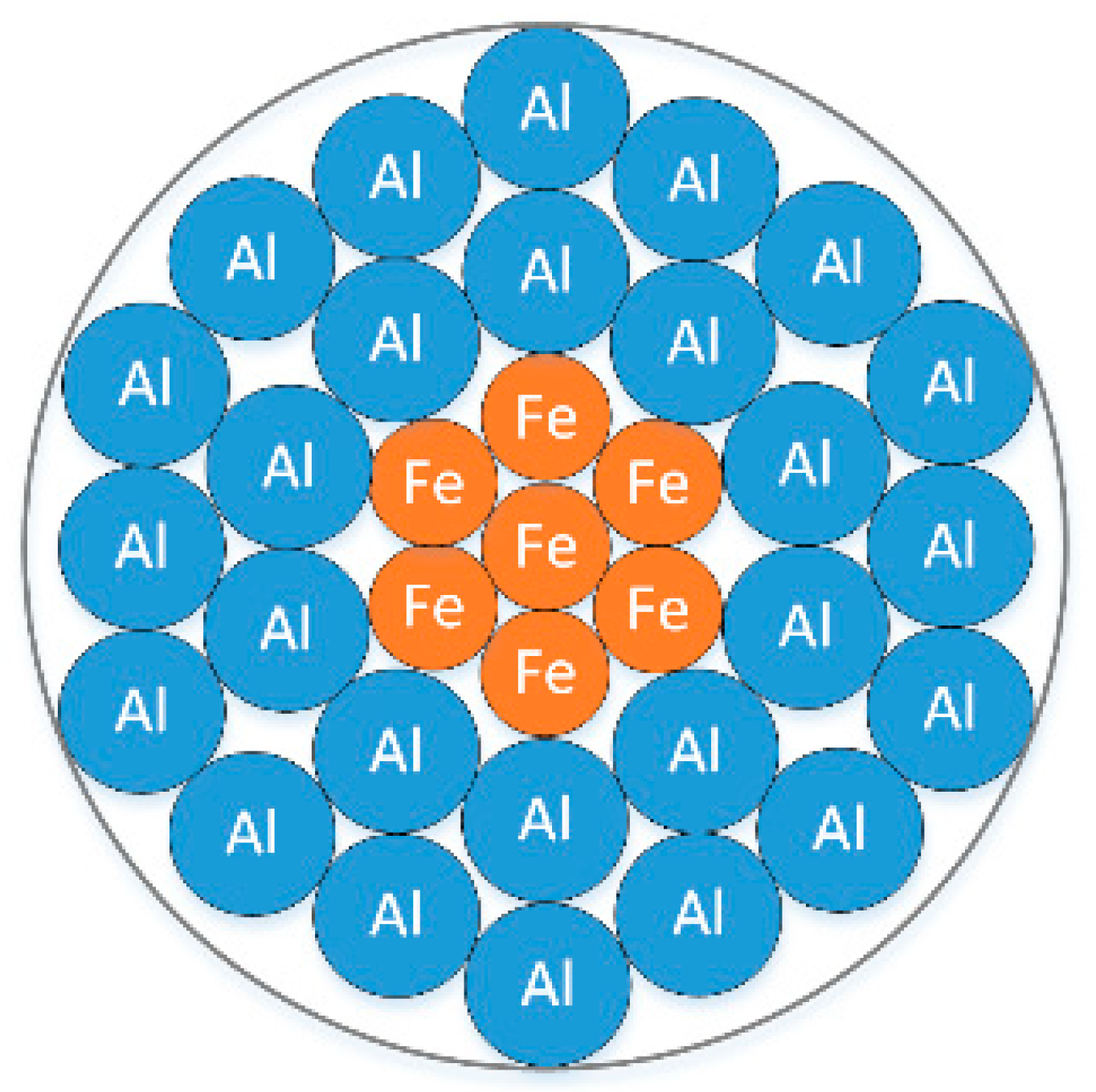
| Number of Al wires | 26 | 54 |
| Number of Al layers | 2 | 3 |
| Diameter of Al wires [mm] | 3.45 | 3.4 |
| Calculated section AAl [mm2] | 243 | 490.3 |
| Number of Fe wires | 7 | 7 |
| Diameter of Fe wires [mm] | 2.68 | 3.4 |
| Calculated section AFe [mm2] | 39.5 | 63.6 |
| Sectional ratio ε’ | 6 | 7.7 |
| Outer diameter of the conductor d [mm] | 21.8 | 30.6 |
| Weight of the conductor [kg/km] | 990 | 1866 |
| Mean Value | Maximum Value | |
|---|---|---|
| Environmental temperature Tenv [°C] | −1.38 | −0.50 |
| Conductor current Icond [A] | 1142.95 | 1308.46 |
| Solar radiation H [W/m2] | 11.97 | 30.30 |
| Wind velocity vwind [m/s] | 0.44 | 1.67 |
| Mean Value | Maximum Value | |||||
|---|---|---|---|---|---|---|
| Conductor AlFe 240/40 | Measurement 1 | Operating temperature [°C] | 60 | Tenv [°C] | 10.98 | 11.41 |
| Season | Autumn | Icond [A] | 725.25 | 904.88 | ||
| Time of measurement | 7:48 to 16:25 | H [W/m2] | 37.27 | 120.91 | ||
| Duration of measurement | 8 h and 36 min | vwind [m/s] | 0.48 | 1.19 | ||
| Measurement 2 | Operating temperature [°C] | 80 | Tenv [°C] | 31.12 | 34.3 | |
| Season | Summer | Icond [A] | 759.04 | 902.77 | ||
| Time of measurement | 9:00 to 16:35 | H [W/m2] | 747.54 | 894.27 | ||
| Duration of measurement | 7 h and 35 min | vwind [m/s] | 0.82 | 2.33 | ||
| Conductor AlFe 490/65 | Measurement 3 | Operating temperature [°C] | 60 | Tenv [°C] | −1.38 | −0.5 |
| Season | Winter | Icond [A] | 1142.95 | 1308.46 | ||
| Time of measurement | 9:00 to 16:27 | H [W/m2] | 11.97 | 30.30 | ||
| Duration of measurement | 7 h and 27 min | vwind [m/s] | 0.44 | 1.67 | ||
| Measurement 4 | Operating temperature [°C] | 80 | Tenv [°C] | 32.79 | 35.5 | |
| Season | Summer | Icond [A] | 831.35 | 1192.18 | ||
| Time of measurement | 9:15 to 18:00 | H [W/m2] | 628.46 | 866.64 | ||
| Duration of measurement | 8 h and 45 min | vwind [m/s] | 1.03 | 2.87 |
| Parameter | Value after Optimization | Value before Optimization | ||
|---|---|---|---|---|
| AlFe 490/65 | AlFe 240/40 | AlFe 490/65 | AlFe 240/40 | |
| α20 [1/K] | 0.0052 | 0.0052 | ||
| r20 [Ω/km] | 0.059 | 0.119 | 0.059 | 0.119 |
| β | 0.51 | 0.27 | ||
| Nu | 16.55 | 15 | ||
| ε | 0.57 | 0.23 | ||
| Duration Time [min] | Temperature [°C] | ||
|---|---|---|---|
| Measured | Model-Calculated | ||
| Identified Parameters | Catalogue Parameters | ||
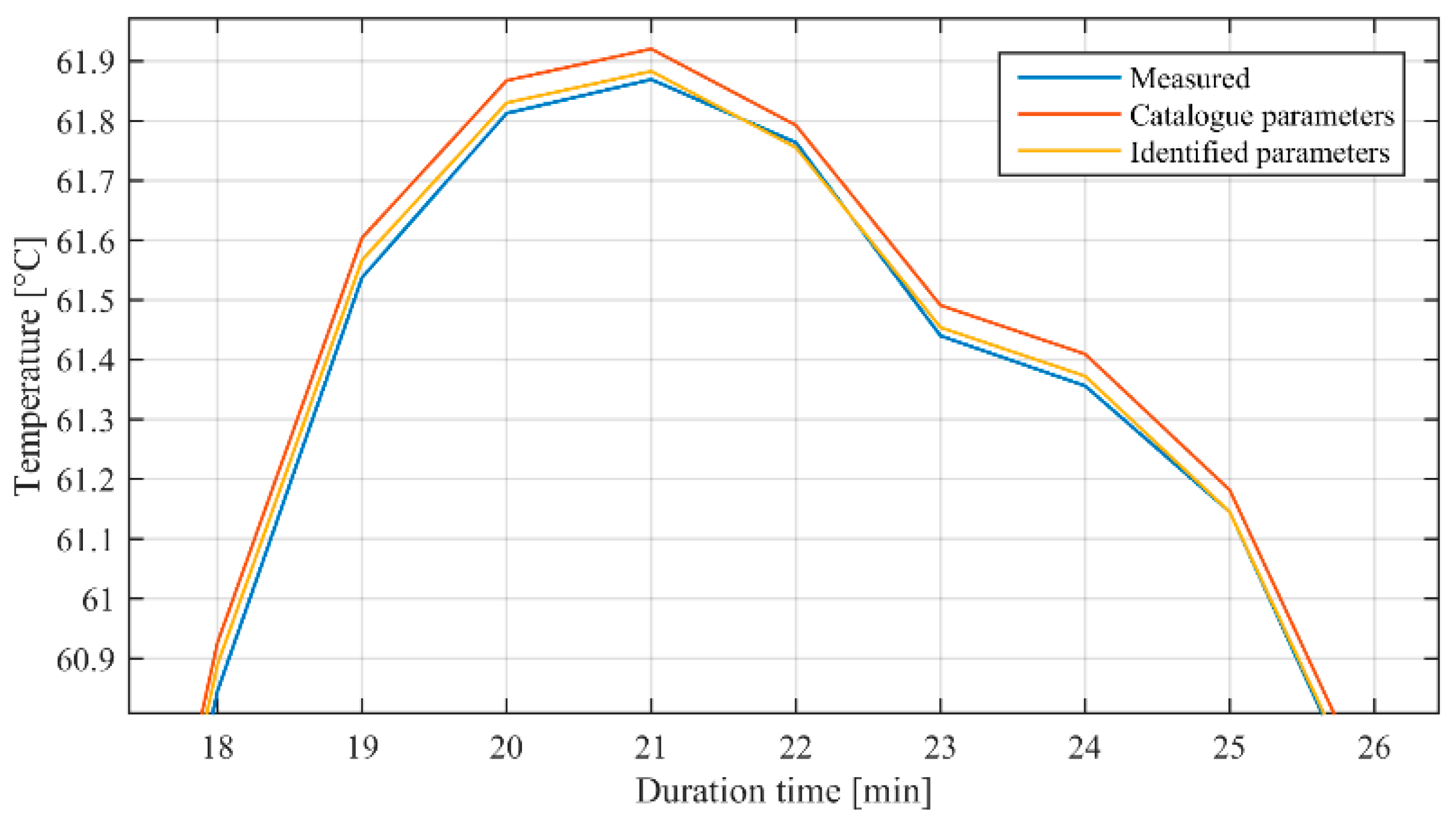
| 18 | 60.84 | 60.89 | 60.93 |
| 19 | 61.54 | 61.57 | 61.60 |
| 20 | 61.82 | 61.83 | 61.87 |
| 21 | 61.87 | 61.88 | 61.92 |
| 22 | 61.76 | 61.75 | 61.79 |
| 23 | 61.44 | 61.45 | 61.49 |
| 24 | 61.35 | 61.37 | 61.41 |
| 25 | 61.14 | 61.14 | 61.18 |
| 26 | 60.62 | 60.62 | 60.66 |
| Operating Temperature 60 °C | Mean Value | Maximum Value | |||||
|---|---|---|---|---|---|---|---|
| Meas. | Calc. | |Meas. − Calc.| | Meas. | Calc. | |Meas. − Calc.| | ||
| AlFe 490/65 | Ts [°C] | 55.42 | 55.41 | 0.01 | 60.69 | 60.67 | 0.02 |
| Pj [p.u.] | 1 | 1 | 0 | 1 | 1 | 0 | |
| Ps [p.u.] | 1 | 1.01 | 0.01 | 1 | 1.01 | 0.01 | |
| Pc [p.u.] | 1 | 0.97 | 0.03 | 1 | 0.97 | 0.03 | |
| Pr [p.u.] | 1 | 1.14 | 0.14 | 1 | 1.13 | 0.13 | |
| AlFe 240/40 | Ts [°C] | 56.74 | 56.74 | 0 | 61.87 | 61.88 | 0.01 |
| Pj [p.u.] | 1 | 1 | 0 | 1 | 1 | 0 | |
| Ps [p.u.] | 1 | 1.01 | 0.01 | 1 | 1.01 | 0.01 | |
| Pc [p.u.] | 1 | 0.97 | 0.03 | 1 | 0.97 | 0.03 | |
| Pr [p.u.] | 1 | 1.13 | 0.13 | 1 | 1.13 | 0.13 | |
| Operating Temperature 80 °C | Mean Value | Maximum Value | |||||
|---|---|---|---|---|---|---|---|
| Meas. | Calc. | |Meas. − Calc.| | Meas. | Calc. | |Meas. − Calc.| | ||
| AlFe 490/65 | Ts [°C] | 70.85 | 70.86 | 0.01 | 81.08 | 81.07 | 0.01 |
| Pj [p.u.] | 1 | 1 | 0 | 1 | 1 | 0 | |
| Ps [p.u.] | 1 | 1.01 | 0.01 | 1 | 1.01 | 0.01 | |
| Pc [p.u.] | 1 | 0.97 | 0.03 | 1 | 0.97 | 0.03 | |
| Pr [p.u.] | 1 | 1.13 | 0.13 | 1 | 1.14 | 0.14 | |
| AlFe 240/40 | Ts [°C] | 78.39 | 78.42 | 0.03 | 81.54 | 81.56 | 0.02 |
| Pj [p.u.] | 1 | 1 | 0 | 1 | 1 | 0 | |
| Ps [p.u.] | 1 | 1.01 | 0.01 | 1 | 1.02 | 0.02 | |
| Pc [p.u.] | 1 | 0.97 | 0.03 | 1 | 0.97 | 0.03 | |
| Pr [p.u.] | 1 | 1.14 | 0.14 | 1 | 1.14 | 0.14 | |
| AlFe 240/40 at 60 °C | Mean Value | Maximum Value | ||||
|---|---|---|---|---|---|---|
| Meas. | Calc. | |Meas. − Calc.| | Meas. | Calc. | |Meas. − Calc.| | |
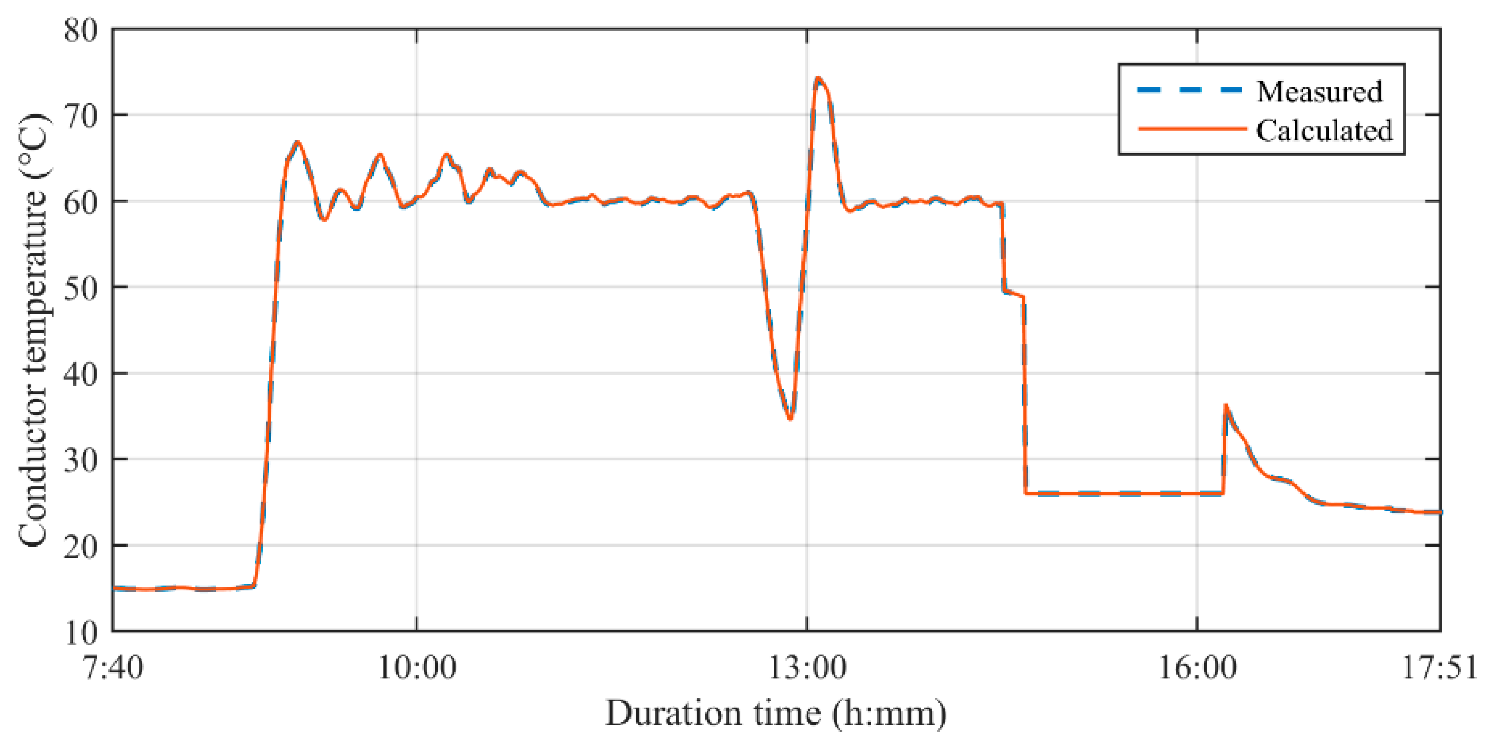
| Ts [°C] | 43.92 | 43.97 | 0.05 | 74.31 | 74.43 | 0.12 |
| Pj [p.u.] | 1 | 1 | 0 | 1 | 1 | 0 |
| Ps [p.u.] | 1 | 1.02 | 0.02 | 1 | 1.02 | 0.02 |
| Pc [p.u.] | 1 | 0.97 | 0.03 | 1 | 0.97 | 0.03 |
| Pr [p.u.] | 1 | 1.14 | 0.14 | 1 | 1.14 | 0.14 |
© 2018 by the authors. Licensee MDPI, Basel, Switzerland. This article is an open access article distributed under the terms and conditions of the Creative Commons Attribution (CC BY) license (http://creativecommons.org/licenses/by/4.0/).
Share and Cite
Sarajlić, M.; Pihler, J.; Sarajlić, N.; Štumberger, G. Identification of the Heat Equation Parameters for Estimation of a Bare Overhead Conductor’s Temperature by the Differential Evolution Algorithm. Energies 2018, 11, 2061. https://doi.org/10.3390/en11082061
Sarajlić M, Pihler J, Sarajlić N, Štumberger G. Identification of the Heat Equation Parameters for Estimation of a Bare Overhead Conductor’s Temperature by the Differential Evolution Algorithm. Energies. 2018; 11(8):2061. https://doi.org/10.3390/en11082061
Chicago/Turabian StyleSarajlić, Mirza, Jože Pihler, Nermin Sarajlić, and Gorazd Štumberger. 2018. "Identification of the Heat Equation Parameters for Estimation of a Bare Overhead Conductor’s Temperature by the Differential Evolution Algorithm" Energies 11, no. 8: 2061. https://doi.org/10.3390/en11082061