An Electric Bus Power Consumption Model and Optimization of Charging Scheduling Concerning Multi-External Factors


1
State Key Laboratory of Alternate Electrical Power System with Renewable Energy Sources, North China Electric Power University, Baoding 071003, China
2
Department of Automation, North China Electric Power University, Baoding 071003, China
3
College of Electrical Engineering, Zhejiang University, Hangzhou 310027, China
4
Energy Research Institute, Academy of Macroeconomic Research, NDRC, Beijing 100038, China
*
Authors to whom correspondence should be addressed.
Energies 2018, 11(8), 2060; https://doi.org/10.3390/en11082060
Submission received: 24 July 2018
/
Revised: 6 August 2018
/
Accepted: 6 August 2018
/
Published: 8 August 2018
Abstract
:With the large scale operation of electric buses (EBs), the arrangement of their charging optimization will have a significant impact on the operation and dispatch of EBs as well as the charging costs of EB companies. Thus, an accurate grasp of how external factors, such as the weather and policy, affect the electric consumption is of great importance. Especially in recent years, haze is becoming increasingly serious in some areas, which has a prominent impact on driving conditions and resident travel modes. Firstly, the grey relational analysis (GRA) method is used to analyze the various external factors that affect the power consumption of EBs, then a characteristic library of EBs concerning similar days is established. Then, the wavelet neural network (WNN) is used to train the power consumption factors together with power consumption data in the feature library, to establish the power consumption prediction model with multiple factors. In addition, the optimal charging model of EBs is put forward, and the reasonable charging time for the EB is used to achieve the minimum operating cost of the EB company. Finally, taking the electricity consumption data of EBs in Baoding and the data of relevant factors as an example, the power consumption prediction model and the charging optimization model of the EB are verified, which provides an important reference for the optimal charging of the EB, the trip arrangement of the EB, and the maximum profit of the electric public buses.
1. Introduction
In recent years, more and more attention has been paid to energy and environment problems such as global energy shortages, serious pollution, and global climate change. Electric vehicles (EVs) have unparalleled advantages in alleviating the energy crisis, improving the environmental pollution, and promoting the harmonious development of humans and the environment [1]. With strong international support and promotion, the EV industry of numerous countries around the world has entered a period of rapid development. In China, the Ministry of Science and Technology released the 12th Five-Year special plan for the development of EV technology pointing out that EVs are mainly demonstrated in buses and taxis, and by 2020, the number of new energy city buses will reach 200,000 [2,3]. The energy demand of the transport sector has been increasing constantly in recent years, consuming one third of the total final energy demand in the European Union over the last decade [4]. Regarding the service and durability of EBs, [5,6] separately study the public service capacities of EV charging as well as battery swapping and costs of city EBs during their service life compared with diesel buses. As for the factors influencing EBs, many scholars have studied such a field. In [7,8], the various factors that influence EBs’ power consumption model is analyzed. The above analysis shows that the current research is less involved in the influence of external factors. In recent years, hazy weather has become serious in China. According to statistics, in 2016, the number of days that Beijing PM2.5 was not up to standard was 168 days, accounting for 46% of the whole year, and heavy pollution accounted for 39 days, most occurring in autumn and winter [9]. The selection of similar days is a popular way to forecast EBs’ power consumption. Some examples of selection of similar days in short-term forecasting and load forecasting problems are as follows: in [10,11,12] the selection of similar days from the perspective about correlation and wavelet analysis in a pre-processing stage, an extreme learning machine dealing with the different factors, a new forecast algorithm, was studied.
The charging cost of the EBs has a great effect on the benefits of the bus company. Therefore, the study of charging optimization models is of vital importance. Recently, many studies have been carried out. Reference [13] proposed the stage of charge (SOC) estimation method based on an Extended Kalman Filter and nonlinear battery model to optimize the charging cost. The mixed-integer linear programming is proposed to optimize the model upon the Charging Promoting Potential of passenger EVs in [14]. Reference [15] presents an energy management and control system of an EV charging station which is designed for charging and discharging of five different plug-in hybrid electric vehicles. As for the optimization strategy of the charging station, [16] proposed a bi-level optimization strategy for the charging load; [17] proposed an EV scheduling method in a power market environment; [18] takes the effect of renewable energy resources, and demand response programs into consideration; in addition, a rolling optimization strategy based on the model and the electricity spot prices is proposed in [19]. Furthermore, under the new circumstance of energy management, the stochastic dynamic programming can be a method to optimize the energy management of a plug-in hybrid electric bus in [20], when solving such problems, a hybrid evolutionary algorithm, is proposed to solve the proposed a multi-objective energy management [21]. The above research focuses on the analysis of power consumption factors, or focuses on the charging optimization model of EVs.
On the basis of the survey data, a power consumption model concerning multi-factors is constructed which can be fitted with actual situation more accurately. Then, the EB charging optimization is put forward, to achieve the optimal cost for the bus company. Finally, from the EB operators scale data for Baoding, Hebei Province, the establishment of an EB power consumption model together with the charging optimization model with the characteristics of time sharing prices into consideration, the optimization upon EBs charging arrangement is studied to reduce the costs of bus companies, which provides a reference for the operation and dispatching of EBs.
2. Selection of Similar Days Considering Fuzzy Evaluation and Analysis of Influencing Factors
2.1. Fuzzy Evaluation of the Feature Library of Influence Factors
2.1.1. Establishment of Power Consumption Feature Library
First, the historical load is analyzed, and the main factors that affect the historical load are identified, and these main influencing factors constitute the daily eigenvectors of historical load. The main influencing factors are converted into numerical values through fuzzy rules [22]. According to the above research information on the factors influencing electric buses’ power consumption, fuzzy quantitative analysis and processing of all factors are carried out. The main factors that affect the power consumption include: travel date (working day or weekend), travel weather condition (temperature, haze or rain), length of travel path, vehicle air conditioning, vehicle running limit policy, etc.
2.1.2. Fuzzy Quantification of Influencing Factors
The results of each feature are shown in Table 1.
2.2. Selection of Similar Days Based on Improved Grey Relational Analysis (GRA)
The influence factors of similar day sets are extracted to form sub vector V, and the improved grey correlation analysis method is used to select similar days [23]. The steps are as follows:
(a) To construct the sub eigenvector matrix V. V is matrix with m × (n + 1) dimensional, m represents the number of days characteristic vectors, n represents rough set number of samples, V0 represents the sub eigenvector of the predicted date:
where, Vi(k) represents the kth characteristic vector of the ith day rough set samples, V0(k) represents the kth component of the sub eigenvector in the predicted date;
(b) Standardized the sub characteristic vector matrix V, and obtained the normalized sub eigenvector matrix V′. In the formula (2), to the normalized eigenvector matrix V′:
where, V′i(k) represents the kth standard sub-eigenvector of the ith rough set;
(c) Solve the difference matrix ΔV′ of the normalization sub eigenvector matrix V′, According to Equation (3), the subcharacteristic vector difference matrix ΔV′ together with ΔV′, ΔV′max, ΔV′min is deduced:
where, ΔV′0(k) represents the kth standard sub eigenvector of the predicted date, ΔV′i(k) represents the kth standard sub feature vector of the rough set sample on the ith day, ΔV0i(k) represents the difference between the kth standard sub feature vector of the rough set sample on the ith day and the kth standard sub eigenvector of the predicted date;
(d) Calculate the correlation coefficient matrix of the sub eigenvector ξ:
where, ξ0i(k) is the kth correlation coefficient vector of the ith rough set sample in the ith day, and ρ ∈ [0,1] is the set resolution coefficient;
(e) Calculate weighted vectors α by correlation coefficient method:
where, βk is the correlation coefficient about the kth component, αk is the weighted correlation coefficient about the kth component, SVi(k)y, SVi(k)Vi(k) separately represent the covariance and variance of the relative factor Vi(k) and daily average power consumption vector y;
(f) Calculate the weighted correlation of the rough set samples:
where, y0i is the weighted correlation degree;
(g) According to the calculated weighted correlation degree, the similar day sample for the expected date is determined. In this paper, a similar day set is obtained by selecting all the daily samples with weighted correlation degree greater than 0.8 when selecting similar days to be predicted.
3. Adaptive Wavelet Neural Network (WNN) Power Consumption Prediction Model Considering Multiple Factors
WNN [24] is used to train and learn the data of power consumption and influencing factors of EBs.
3.1. An Overview of WNN
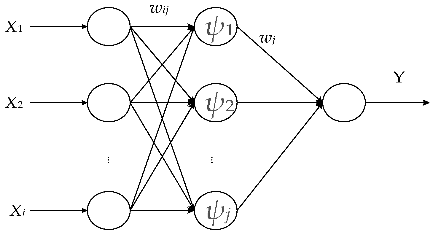
WNN is a kernel function neural network formed by combining the multi-scale resolution of the wavelet theory with the good local characteristics of the time domain and the self-learning ability of the neural network in the reinforcement learning. The topology structure of the neural network is depicted in Figure 1, and the transmission function of the hidden layer nodes is a small wave base function. Wavelet analysis and BP network have strict mathematical theoretical background. Besides, in addition to adjusting the weights and thresholds of the network, the WNN can also adjust the expansion factor and translation factor of the wavelet function, which has more sensitive approximation ability and more error tolerant ability than the BP neural network.
3.2. Training and Learning of WNN
Let ψ(t) ∈ L2 *(R) be a wavelet basis function, and ψ(t) satisfy the admissibility condition:
where, ψ(ω) is the Fourier transform of ψ(t); and ψ(t) is a group of small wave base functions are generated after the translational expansion.
The topology of the wavelet neural network model is shown in Figure 1.
In Figure 1, Xi (i = 1, 2, …, t) is the input sequence of WNN, Y is an output sequence; wij the weight of the connection between the input layer and the hidden layer, and wj is the connection weight between the hidden layer and the output layer. When the input signal sequence is xi (i = 1, 2, …, t), the output formula of the hidden layer is as follows:
where, g(j) is the output of the jth node of the hidden layer; ψj is a small wave base function; aj is the expansion factor of ψj; the λj is the translation factor of ψj, wij the weight of the connection between the input layer and the hidden layer, and the formula for the calculation of the output layer is:
where, l is the number of hidden layer nodes, wj is the connection weight between the hidden layer and the output layer.
3.3. The Prediction Process of WNN
(1) Random initialization—the weights of input to the hidden layer in the wavelet neural network with random initialization are w0ij, the hidden layer to the output layer weight w0jk, and the wavelet basis function expansion factor b0j;
(2) Set the parameters of the estimated link network structure: concerning the number of input neurons is N, the number of neurons in hidden layer is Nh, and the number of output neurons is M;
(3) Set prediction link network fitting error reference value e and maximum iteration number Nd;
(4) Adopt the known historical electric bus power consumption data for supervised learning, the parameters wkij, wkjk, bkj, θkj with strong fitting ability for electricity data are obtained;
(5) Based on wkij, wkjk, bkj, θkj, adopt the prediction link to predict, input the n time (such as 15 min), the actual history output data is X01, X02, …, X0n, get the next M time (such as 15 min) output estimate value Y01, Y02, …, Y0m;
(6) In the sampling period between two adjacent prediction time ij, measured data Pi1, Pi2, …, Pin and the ith period network state parameters wkij, wkjk, bkj, θkj are used as input parameters for topology optimization;
(7) The network online training approximation performance index J(t) is evaluated. Online training is performed to approximate optimal control Δw*ij, Δw*jk, Δb*j, Δθ*j; another network weight is fixed when a network parameter is trained, and the related methods can be seen in the literature [25];
(8) The new state parameter w*ij, w*jk, b*j, θ*j replace state parameter wkij, wkjk, bkj, θkJ in the ith period, the input value is Pi1, Pi2, …, Pin, the output value is Y*1, Y*2, …, Y*m;
(9) Y*1, Y*2, …, Y* is the optimal predictive value;
(10) End.
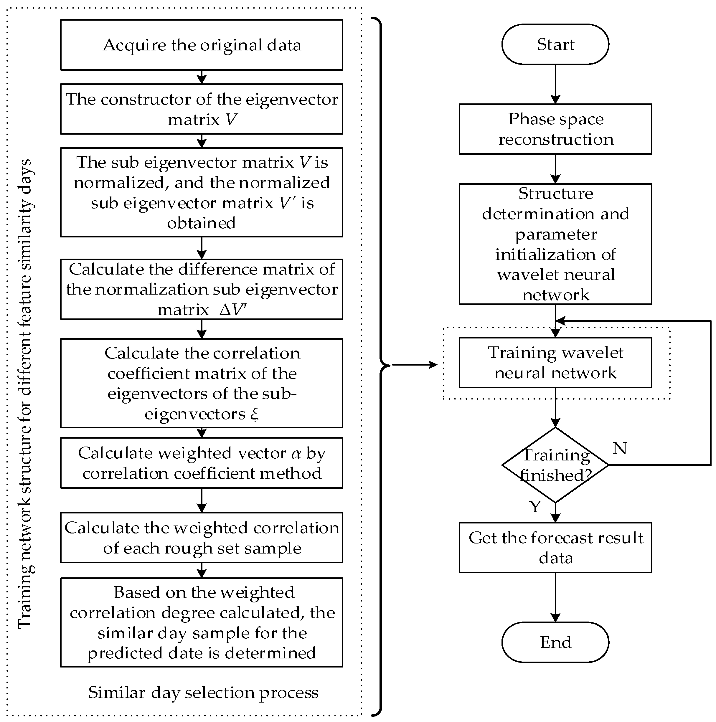
The basic prediction steps in this paper are shown in Figure 2.
4. Establishment of Charging Optimization Model for Electric Buses
With the vigorous development of China’s EV industry, the state has adopted the policy of supporting EBs, and also encourages the construction of charging facilities for EBs. Battery charging stations act as the battery charging hub, the position of charge for power distribution and service network capacity are closely related, but the partial public bus charging facilities are allocated more regularly, which is slightly different from conventional EV charging piles in the allocation process.
4.1. Optimization Research Model of EBs
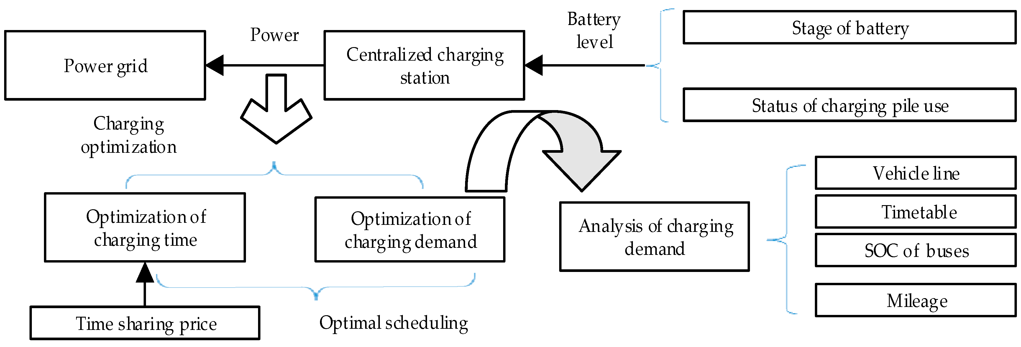
Nowadays, battery replacement is the most extensively used method for charging electric buses. With the continuous improvement and development of battery technology and the rapid rise of fast charging technology, the fast speed of fast charging pile brings great convenience to EVs and has been widely receiving extensive popularity. The good interactive characteristics between the electric bus and the power grid, and its rational optimization can achieve the maximum benefit for the bus company. The basic operation and scheduling model is shown in Figure 3.
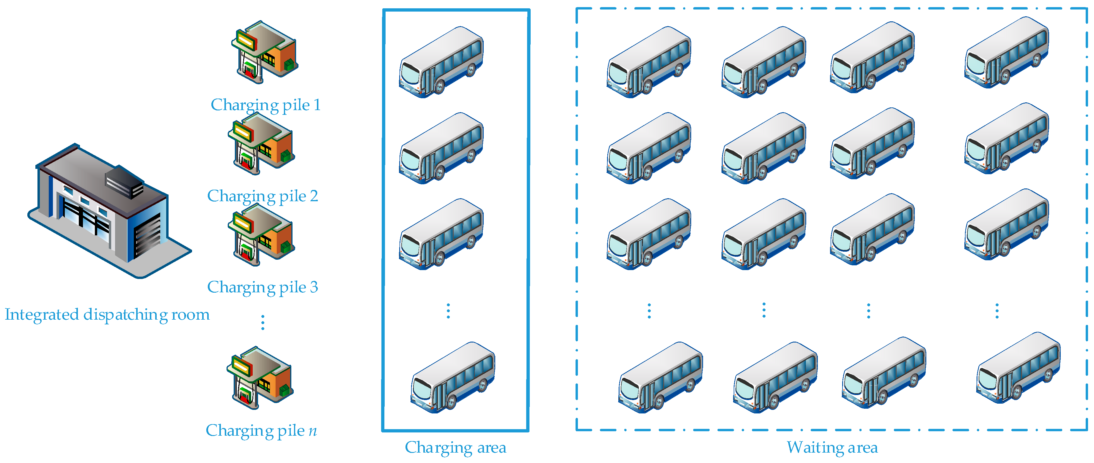
This study adopted a fast charging, direct analysis of the electric bus queue charging mode. In addition, in view of China’s general implementation up on time of use (TOU) price, it can be optimized in the process of charging optimization of EBs. For EB charging and charging station configuration, the following module structure is adopted, including charging pile, auxiliary equipment room of charging pile, comprehensive dispatching room of charging station, vehicle charging area, waiting area of vehicles waiting for charging, etc. And the basic structure diagram is shown in Figure 4.
The above module is a research model, and the conclusion of the research can be extended to the whole EB industry. The charging optimization of EB is described detail in the following section.
4.2. Optimization Goal
The optimal dispatching of electric buses is mainly based on vehicles’ travel rules, charging mode, charging price of the power system, and power consumption characteristics of electric buses. The study assumes that the capacity of the charging station is fixed. Considering the high cost of the charging stations, only the electric charge paid by the bus company during the operation process and the operation and maintenance cost of the charging pile is calculated in the optimization process, by optimizing the number of charging vehicles and charging piles at different times, to acquire the lowest cost of the bus company. Therefore, the charging of EBs need to be arranged. Considering the TOU price in Baoding, China, that is to say, different charging arrangements will bring different costs to the bus company, which is bound to have a lowest cost charging scheme. This paper is the research on the optimal scheduling of electric bus companies under the above conditions.
The optimization goal of EB charging scheduling is:
where, αt, γt are logical variables 0, 1, αtj = 1 stands for the jth EB is under charged at t time, while αtj = 0 stands for the corresponding electric bus is not charged; p presents the power of the charging generator, price(t) is the TOU price at t time; N is the number of charging electric buses; Δt is designed time window set to 15 min; γi = 1 stands for the ith charging pile is under, otherwise is not under used; m stands for maintenance cost of charging pile in a day; Number is the number of the total available charging pile.
4.3. Constraint Condition
(1) Charge and discharge balance constraint in a whole day
where, βtj = 1 indicates the jth electric bus is in the stage of work at t time, otherwise, it means that the electric bus is not working;
(2) Initial state constraints of power batteries:
In the equation, the battery storage energy of every day is invariable to satisfy the optimal dispatch of electric bus charging in the next day;
(3) Constraint for charging time (to prevent a single charge time too short):
where, th is the single charge time of the electric bus, Δt is designed for the charging time window in this paper, which is set to 15 min;
(4) The mutual exclusion constraint of the electric bus (that is, every bus cannot be in the state of both charging and discharging):
(5) Upper and lower bound constraints that SOC should meet in the charging process of an electric bus [26]:
where, SOCmin = 0.2, SOCmax = 0.9. Among them, the minimum mainly take the standby capacity and the return capacity into consideration in the operation of the electric bus [23];
(6) Constraint upon travel times of electric buses:
where, h is the total time length of operation in one day, Δt is the charging time window (equal to the departure time window) designed as 15 min, M is the total number of times for the electric bus;
(7) The limit of the number of electric buses charging:
where, take the jth bus as an example, is a logical operation symbol, stands for XOR (exclusive or) and the state of a charging process is turned over two times, Ncharge is the limit of the number of charges in one day.
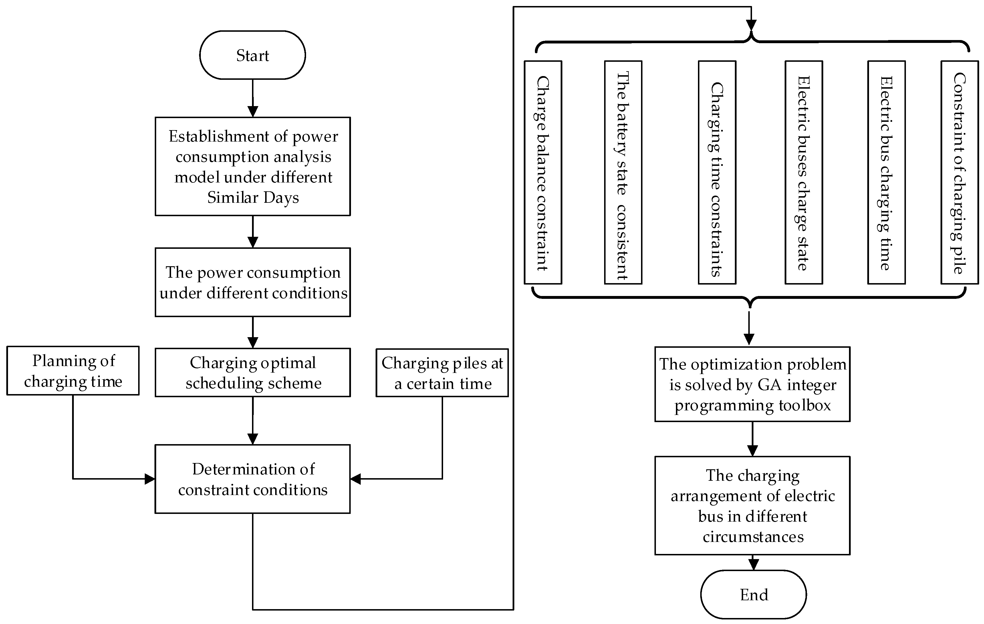
4.4. Solution of Optimal Model
The optimization model established above is a typical integer programming problem. In order to optimize the solution of charging scheduling, the genetic algorithm (GA) integer optimization toolbox is used to solve the optimization problem. The framework of the model solution is shown in Figure 5.
5. Case Study
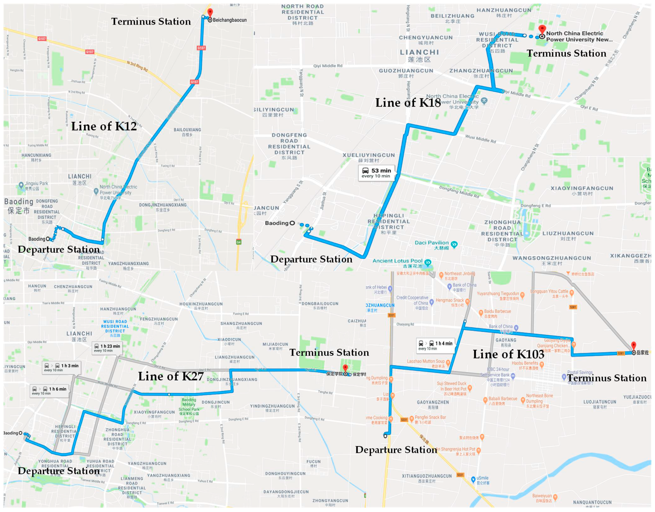
This paper investigates the related situation of EBs in Baoding, Hebei Province. In 2015, Baoding bought 591 EBs and put them into operation at the end of the year, representing about 80% of the bus operation tasks in the city, and the daily average mileage of the EBs is 80 km. This case takes the K12, K18, K27 and K103 buses as an example, and forecasts the daily electric buses’ SOC, charging consumption and the 100 km power consumption under different cases. The battery capacity of the electric bus in the example is 171.2 kW h. In order to keep the remaining battery power at 20%, the power consumption of the full charging battery is no more than 70% of the total capacity of the battery, that is, 119.84 kW h. An organic whole charging generator with 105 kW is used in Baoding city electric bus charger charging piles which can provide the constant power charging. The main path of the electric bus is shown in Figure 6.
This investigation and research carries out from the beginning of October 2016, to the end of February 2017, during the period of 1 October 2016 to 14 November without air condition and the electric buses are not limited, the bus fare is 1 yuan; during the period of 15 November–31 December with air condition open and the bus fare is for free; during the period of 1 January 2017–28 February with no traffic limited air condition open the fare is 2 yuan. The investigation is carried out in the way of starting SOC with the car and recording the power consumption of the electric bus. Two days of work day and one day in non-working day are selected, and the survey time is 7:30 a.m.–7:00 p.m.
5.1. Power Consumption Model of Bus Based on the Adaptive WNN
Firstly, according to the characteristics of the above similar days, the classification of the operation scenarios of the electric buses is presented, and the classification results are shown in Table 2.
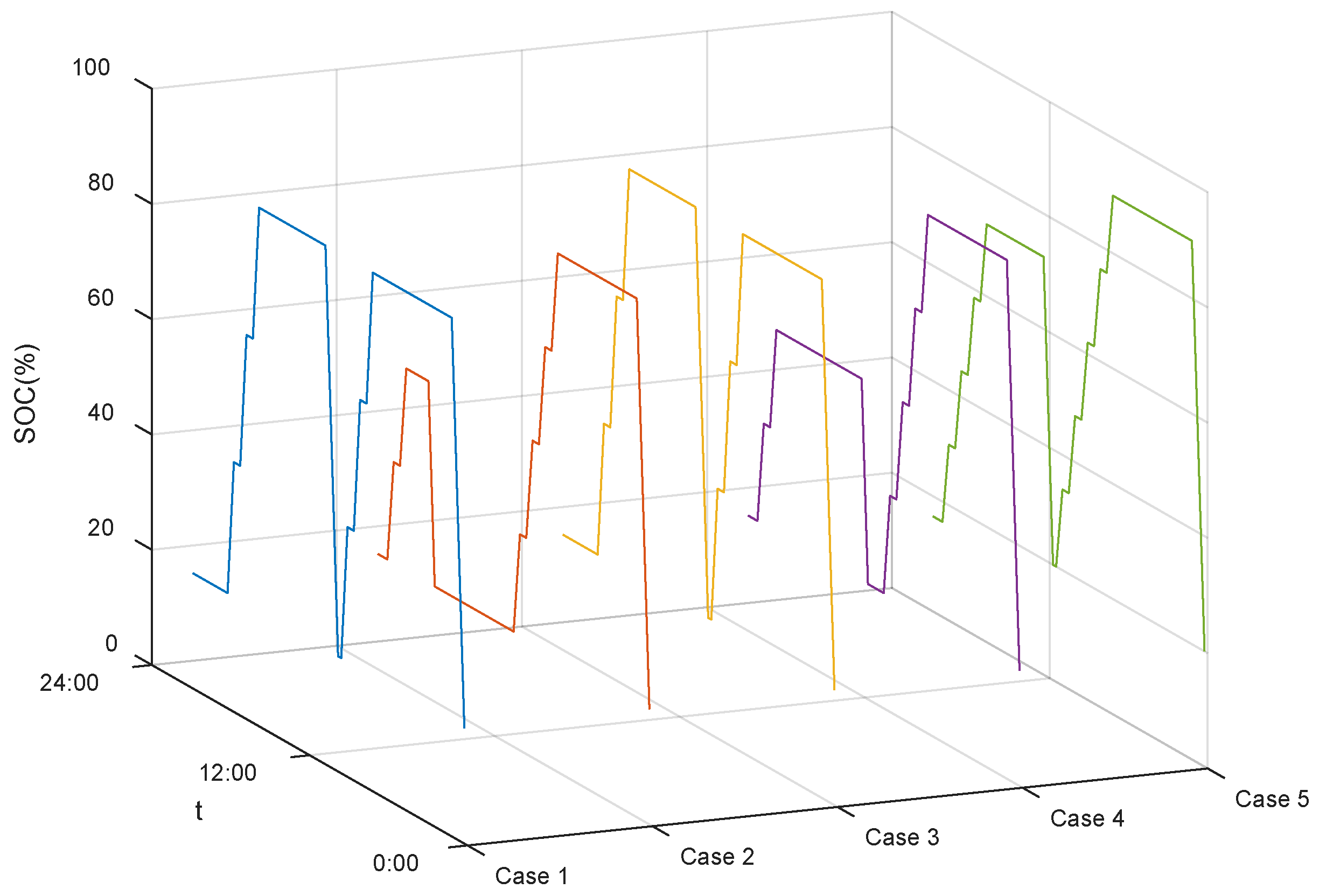
The WNN based on similar day characteristics is established for different running situations, and it is trained according to the statistical historical data of the charging pile, to predict the power consumption of electric bus in different day type. Furthermore, based on the change state of the SOC of the EBs in different situation, as depicted in Figure 7, and then multiplied by the rated capacity of the battery, the daily cumulative electricity consumption and the daily operating mileage can be known. It can be seen that the power consumption of 100 km for the EB is compared with the traditional estimated method. The prediction results of the power consumption forecast model under the evaluation of the influencing factors together with the traditional prediction results are shown in the following Table 3.
Figure 7 represent the charging stage of the SOC upon EB on various similar days, therefore, the electric consumption of EB can be predicted. The prediction results of the power consumption forecast model under the evaluation of the influencing factors together with the traditional prediction results are shown in the following Table 3.
By comparing the forecast results about the power consumption of 100 km, it is clearly that the MAPE of the method concerning the multi-factors is 2.45, which is far lower than the MAPE of the traditional l fixed energy consumption model with the value of 8.03.
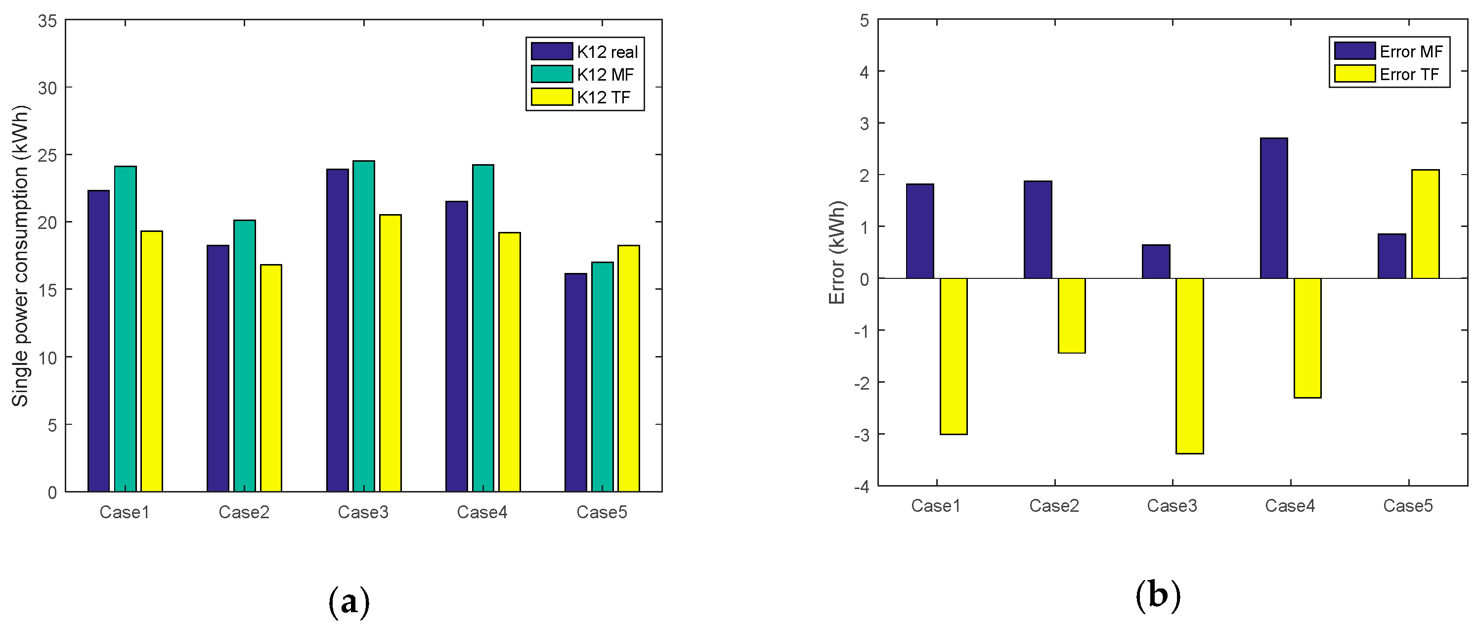
The predictive value of adaptive WNN based on similar day selection (use MF instead) is obtained by using the method in this paper, and the predictive value of traditional fixed energy consumption (use TF instead) is a rough prediction gained by the tradition method (obtain the traditional power consumption forecast from the EB company) based on the TF traditional departure experience without taking the multiple factors into consideration. To make more detailed presentation of the advantages of prediction method concerning the multiple factors, taking K12 bus as an example, the single circle comparison prediction results under different cases are shown below.
The prediction results of the electric bus consumption prediction model with many factors have high accuracy. Figure 8 shows that the accuracy of the power consumption prediction under the consideration of multiple factors is higher and the deviation of the prediction results is consistent (the prediction error is positive); the prediction accuracy of the traditional bus company prediction method is slightly lower and the deviation of prediction results are not consistent, which is mainly reflected in the fact that the prediction error is positive only in Case 5 (no air conditioning or no traffic limited), and the rest are negative. That is to say, under the air conditioning or the limited case, the forecast power consumption is lower than the actual power consumption, and the actual EB travel arrangement cannot be met. In order to meet the actual traffic needs, the fuel vehicles of the bus company have to be put into use, however, it would be contrary to the original intention of environmental protection (such situations always occur under the condition of the air conditioning or the traffic limit, including Case 1, Case 2, Case 3, Case 4). However, the prediction precision obtained from considering the multiple factors can meet the actual requirements, and there is a certain margin, thus ensuring the basic travel needs of the EB. From Figure 8b, it is clear that the prediction deviation can be reduced by about 5% after considering the multi factors. And the corresponding evaluation index MAPE about the line K12 is 7.76 calculated by MF, while the MAPE value is 11.83 calculate by TF, proving that the proposed methods improves the forecast accuracy of the power consumption of the EB.
5.2. Charging Optimization for EB with Different Charging Piles
According to the power consumption of the model of 5.1, the charging of the corresponding optimization is carries out with the EBs days before, that is to meet the situation under the premise of travel demand, bus charging optimization, to achieve the lowest cost of charging. The TOU price carried out upon the EB charging station in Baoding is showed in the following Table 4.
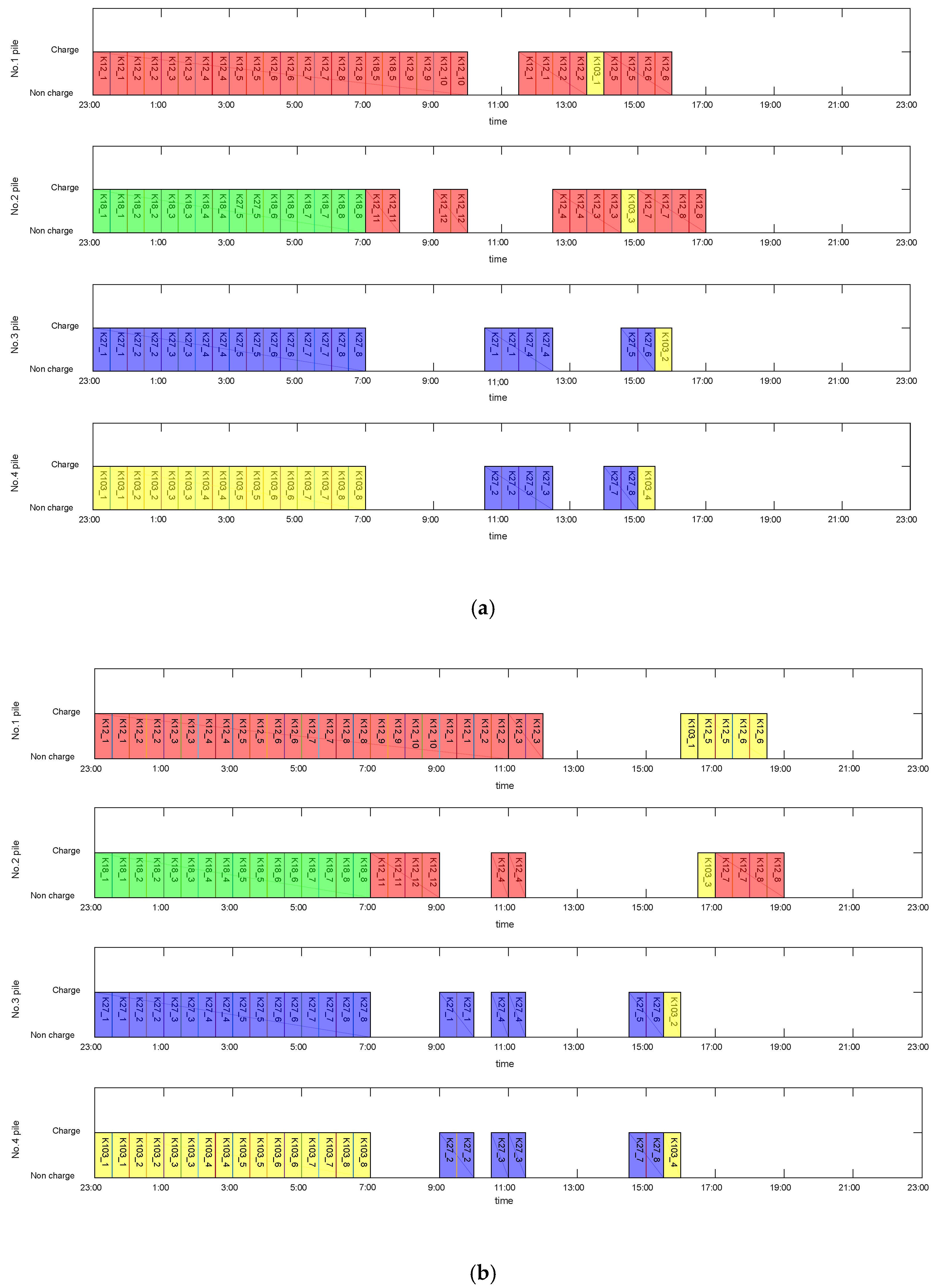
The charging optimization results together with the scheduling of non-optimized charging results are correspondingly present in Figure 9a,b, which stands for the charging stage of four different charging piles in the EB charging station. Taking the four different lines containing K12, K18, K27, K103 as examples to optimize the charging of the EBs with the TOU price into consideration.
5.3. Analysis on the Cost of Optimized Charging
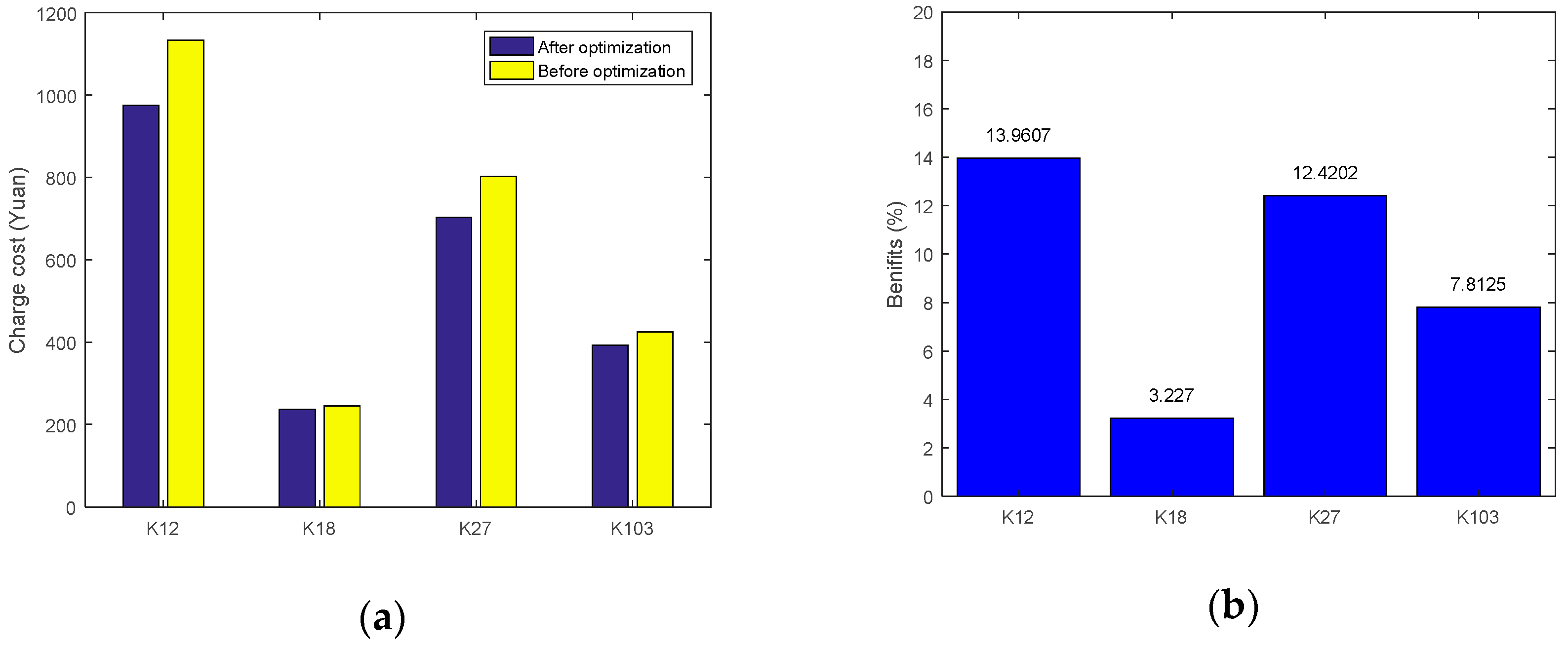
The cost before and after optimization in different cases are shown in the following Figure 10.
Through the comparison of the charging costs of different cases it can be seen that the optimal revenue (percentage) under different cases from high to low is Case 3, Case 1, Case 4, Case 2, Case 5. Compared with other cases, the charging power consumption is the largest under the peak condition of air conditioning and limited traffic (Case 3). More EBs should be put into the optimization of charging and scheduling, the more optimization space is, the greater the benefit of obtaining the optimal cost is. Similarly, under the condition of no air conditioning and no traffic-limit, the profit gained from optimization is relatively small. In this case, more people choose to use private cars rather than EBs for the sake of convenience, which will reduce the power consumption of EBs, therefore, to reduce the cost of charging optimization. When Case 1 comparing with Case 3 (or Case 2 comparing with Case 4), with the condition of the limit to the travel of public cars, and the government’s free bus travel service for the public, which will increase the utilization of EBs, and the space for optimization will become larger. The comparison of Case 1 (and Case 2) with Case 5 shows that the difference between the two is more obvious in the peak situation, and the difference between the two is not obvious in the non-peak situation.
According to the above optimization results and analysis, it can be concluded that: by analyzing the charging cost before and after the optimization in different situations, it can be seen that approximately 10% the charging cost of electricity consumption can be saved by using the optimize charging method proposed considering the TOU price in this paper. Such a study provides a feasible charging optimization way to reduce the cost of EB companies. This is of tremendous importance to the charging optimization, thus accelerating the healthy development of the EB industry.
5.4. Summary for the Case Analysis
On the one hand, the results are displayed by analyzing the power consumption forecast model of EBs which is based on the influence of multivariate factors, and it can be seen that the adaptive WNN forecast model based on similar day selection has higher prediction precision, and its forecast evaluation index value of MAPE is 2.45 which is far lower than the conventional stationary energy consumption methods. The proposed method’s superiority is reflected in considering the influence of multiple external factors, whose prediction shows good consistency, and the actual power consumption will leave a certain margin, to meet the daily operational needs, and improve the precision of prediction and provide the guarantee for the travel of EBs. On the other hand, on the basis of the power consumption forecasting model, the optimized scheduling of the charging piles in the station is optimized taking the TOU price into consideration, and the calculation example verifies that the operating revenue can be increased and the charging cost can be reduced by 10%. This makes tremendous sense on the development of the EB industry and the bus companies’ revenue.
6. Conclusions
In the actual operation of electric public bus companies, the general operation characteristics of electric buses are relatively fixed. Therefore, this article starts by taking an actual survey data into consideration, which combines the running characteristics of the electric bus and considers multiple external influencing factors, the fuzzy evaluation method of the electric bus is adopted to a variety of different influence factors by GRA. Furthermore, a similar day selection model is established, and WNN is used to train the learning factors to predict the power consumption. On the basis of the power consumption prediction, combined with the characteristics of the TOU price in the city, the daily charging of the electric buses is optimized. After establishing the target function, the optimization toolbox of GA is used to solve the optimal model of the electric buses’ charging, and the effectiveness and practicality of the optimized model are verified, with the following advantages:
(1) Based on the historical multiple factors related to power consumption of the electric bus obtained by investigation, the GRA between the power consumption and many influencing factors is carried out by fuzzy evaluation together with similar day selection. The WNN is used to train learning based on the analysis results, and a power consumption prediction model considering multiple factors is established. The change of the SOC of the electric bus before the day is predicted, and the power consumption of the electric bus can be obtained. Compared with the traditional electric bus power consumption prediction method, it can be seen that the prediction accuracy is greatly improved, the prediction deviation can be reduced by about 5% after considering the multi factors.
(2) According to the forecast result of the power consumption of the electric buses, considering the characteristic of the TOU price for the electric bus charging station, the charging scheduling of the electric buses is optimized through the electric bus power consumption characteristics under the different similar day type, which can reduce the operation cost of the electric bus company. About 10% of the cost is saved, which provides a feasible strategy for optimizing the efficiency of electric bus companies and enhancing their competitiveness.
In this paper, considering the different external factors such as hazy weather, limited line policy and air condition use, the EB power consumption forecasting model based on the similar day selection using WNN is established, which can improve the accuracy of prediction and provide the basis and reference for the operation optimization of EBs. On the basis of EB power consumption forecast to guarantee the optimal dispatching of EBs, which is of great significance to improve the operation profit of charging stations and realize the cost optimization of EB charging stations, concerning the TOU electricity price for bus charging.
Author Contributions
Conceptualization, Y.G. and S.G.; Methodology, Y.G. and S.G.; Software, S.G., J.R. and Y.Z.; Validation, S.G., J.R., Y.G. and Z.Z.; Formal Analysis, S.G. and A.E.; Investigation, Y.G., S.G. and J.R.; Resources, Y.G. and S.G.; Data Curation, S.G. and Z.Z.; Writing-Original Draft Preparation, Y.G. and S.G; Writing-Review & Editing, S.G., Y.G. and A.E.; Visualization, Y.G. and S.G.; Supervision, Y.G. and S.G; Project Administration, Y.Z.; Funding Acquisition, Y.G. and Y.Z.
Acknowledgments
This work is supported in part by the Nature Science Foundation of China (51607068), the Beijing Talents Fund (2015000102592G282) and the Fundamental Research Funds for the Central Universities (2018MS082).
Conflicts of Interest
The authors declare no conflict of interest.
Abbreviations
The following abbreviations are used in this manuscript:
| EBs | electric buses |
| GRA | The grey relational analysis |
| SOC | Stage of charge |
| WNN | the wavelet neural network |
| ELM | extreme learning machine |
| GA | genetic algorithm |
| TOU | time of use |
| MF | Multi factors forecast |
| TF | Traditional forecast |
References
- Zhang, P.; Yan, F.; Du, C. A comprehensive analysis of energy management strategies for hybrid electric vehicles based on bibliometrics. Renew. Sustain. Energy Rev. 2015, 48, 88–104. [Google Scholar] [CrossRef]
- A Review of the Development of New Energy Automobile Industry in the Transportation Industry in the Period of “12th Five-Year”. Available online: http://gjss.ndrc.gov.cn/zttp/xyqzlxxhg/201712/t20171221_871251.html (accessed on 21 December 2017).
- Speeding up the Application of New Energy Vehicles in the Transportation Industry. Available online: http://www.mot.gov.cn/jiaotongyaowen/201510/t20151014_1897377.html (accessed on 26 March 2015).
- Dominković, D.F.; Bačeković, I.; Pedersen, A.S.; Krajačić, G. The future of transportation in sustainable energy systems: Opportunities and barriers in a clean energy transition. Renew. Sustain. Energy Rev. 2017, 82, 1823–1838. [Google Scholar] [CrossRef]
- Zhang, T.; Chen, X.; Yu, Z.; Zhu, X.; Shi, D. A Monte-Carlo Simulation Approach to Evaluate Service Capacities of EV Charging and Battery Swapping Stations. IEEE Trans. Ind. Inf. 2018. [CrossRef]
- Lajunen, A.; Lipman, T. Lifecycle cost assessment and carbon dioxide emissions of diesel, natural gas, hybrid electric, fuel cell hybrid and electric transit buses. Energy 2016, 106, 329–342. [Google Scholar] [CrossRef]
- Zhang, X.; Qiushuo, L.I.; Tao, S.; Xiao, X.; Zhao, B. Influence Factors Analysis and Modeling of Power Demand for Electric Bus Charging Station. Mod. Electr. Power 2014, 31, 28–33. [Google Scholar] [CrossRef]
- Wang, M.Y.; Zhang, H.X.; Zhang, T.Z.; Liu, Y. Study on Response Surface Model of Actual Power Consumption of Electric Buses. J. Qingdao Univ. 2014, 29, 49–53. [Google Scholar]
- The Average PM2.5 Concentration Dropped 9.9% Last Year. Available online: http://bjrb.bjd.com.cn/html/2017-01/04/content_94194.htm (accessed on 4 January 2017).
- Bento, P.M.R.; Pombo, J.A.N.; Calado, M.R.A.; Mariano, S. A bat optimized neural network and wavelet transform approach for short-term price forecasting. Appl. Energy 2018, 210, 88–97. [Google Scholar] [CrossRef]
- Sun, W.; Zhang, C. A Hybrid BA-ELM Model Based on Factor Analysis and Similar-Day Approach for Short-Term Load Forecasting. Energies 2018, 11, 1282. [Google Scholar] [CrossRef]
- Dai, S.; Niu, D.; Li, Y. Daily Peak Load Forecasting Based on Complete Ensemble Empirical Mode Decomposition with Adaptive Noise and Support Vector Machine Optimized by Modified Grey Wolf Optimization Algorithm. Energies 2018, 11, 163. [Google Scholar] [CrossRef]
- Stroe, A.I.; Meng, J.; Stroe, D.I.; Świerczyński, M.; Teodorescu, R.; Kær, S.K. Influence of Battery Parametric Uncertainties on the State-of-Charge Estimation of Lithium Titanate Oxide-Based Batteries. Energies 2018, 11, 795. [Google Scholar] [CrossRef]
- Teshigawara, Y.; Ikegami, T. Charging Load Aggregation Potential of Multiple Electric Vehicles Based on Road Traffic Census Data. Electr. Eng. J. 2018, 203, 64–371. [Google Scholar] [CrossRef]
- Mumtaz, S.; Ali, S.; Ahmad, S.; Khan, L.; Hassan, S.Z.; Kamal, T. Energy Management and Control of Plug-In Hybrid Electric Vehicle Charging Stations in a Grid-Connected Hybrid Power System. Energies 2017, 10, 1923. [Google Scholar] [CrossRef]
- Bao, Y.; Luo, Y.; Zhang, W.; Huang, M.; Wang, L.Y.; Jiang, J. A Bi-Level Optimization Approach to Charging Load Regulation of Electric Vehicle Fast Charging Stations Based on a Battery Energy Storage System. Energies 2018, 11, 229. [Google Scholar] [CrossRef]
- Caramanis, M.; Foster, J.M. Management of electric vehicle charging to mitigate renewable generation intermittency and distribution network congestion. In Proceedings of the Joint 48th IEEE Conference on Decision and Control and 28th Chinese Control Conference, Shanghai, China, 16–18 December 2009; pp. 4717–4722. [Google Scholar]
- Bagher Sadati, S.M.; Moshtagh, J.; Shafie-khah, M.; Catalão, J.P.S. Risk-Based Bi-Level Model for Simultaneous Profit Maximization of a Smart Distribution Company and Electric Vehicle Parking Lot Owner. Energies 2017, 10, 1714. [Google Scholar] [CrossRef]
- Kong, F.; Jiang, J.; Ding, Z.; Hu, J.; Guo, W.; Wang, L. A Personalized Rolling Optimal Charging Schedule for Plug-In Hybrid Electric Vehicle Based on Statistical Energy Demand Analysis and Heuristic Algorithm. Energies 2017, 10, 1333. [Google Scholar] [CrossRef]
- Li, L.; Yan, B.; Yang, C.; Zhang, Y.; Chen, Z.; Jiang, G. Application oriented stochastic energy management for plug-in hybrid electric bus with AMT. IEEE Trans. Veh. Technol. 2016, 65, 4459–4470. [Google Scholar] [CrossRef]
- Azizivahed, A.; Naderi, E.; Narimani, H.; Fathi, M.; Narimani, M.R. A new bi-objective approach to energy management in distribution networks with energy storage systems. IEEE Trans. Sustain. Energy 2018, 9, 56–64. [Google Scholar] [CrossRef]
- Krasopoulos, C.T.; Beniakar, M.E.; Kladas, A.G. Multi-Criteria PM Motor Design based on ANFIS evaluation of EV Driving Cycle Efficiency. IEEE Trans. Transp. Electrif. 2018. [CrossRef]
- Khan, M.S.A.; Abdullah, S. Interval-valued Pythagorean fuzzy GRA method for multiple-attribute decision making with incomplete weight information. Int. J. Intell. Syst. 2018, 33, 1689–1716. [Google Scholar] [CrossRef]
- Santhosh, M.; Venkaiah, C.; Kumar, D.M.V. Ensemble empirical mode decomposition based adaptive wavelet neural network method for wind speed prediction. Energy Convers. Manag. 2018, 168, 482–493. [Google Scholar] [CrossRef]
- Si, J.; Wang, Y.T. Online learning control by association and reinforcement. IEEE Trans. Neural Netw. 2001, 12, 264–276. [Google Scholar] [CrossRef] [PubMed] [Green Version]
- Abdalrahman, A.; Zhuang, W. A Survey on PEV Charging Infrastructure: Impact Assessment and Planning. Energies 2017, 10, 1650. [Google Scholar] [CrossRef]
- Yang, Y.; Zechun, H.U.; Song, Y. Research on Optimal Operation of Battery Swapping and Charging Station for Electric Buses. Proceed. CSEE 2012, 32, 35–42. [Google Scholar]
Figure 1.
Topology of wavelet neural network.

Figure 2.
Prediction flow chart of WNN based on similar day selection.

Figure 3.
Scheduling operation of charging station.

Figure 4.
Optimization submodule structure diagram of charging station charging facilities.

Figure 5.
Frame flow chart of power consumption analysis and electric buses charging optimization.

Figure 6.
Investigation of road route map of bus line.

Figure 7.
Day-head SOC curves of electric buses under different cases.

Figure 8.
The comparison prediction results in the single circle under various cases (a) The comparison prediction of true value; (b) The comparison of forecast error.
Figure 8.
The comparison prediction results in the single circle under various cases (a) The comparison prediction of true value; (b) The comparison of forecast error.

Figure 9.
(a) Electric buses scheduling without charging optimization of Case 3; (b) Electric buses scheduling without charging optimization of Case 3.
Figure 9.
(a) Electric buses scheduling without charging optimization of Case 3; (b) Electric buses scheduling without charging optimization of Case 3.

Figure 10.
(a) Charging cost before and after optimization under different cases; (b) The percentage of optimal benefits in different cases.
Figure 10.
(a) Charging cost before and after optimization under different cases; (b) The percentage of optimal benefits in different cases.


Table 1.
Fuzzy rule of daily characteristic vectors.
| Characteristic Quantity | Fuzzy Quantization Rule |
|---|---|
| Day type (D) | Tue. to Fri. set to 1; Sat., Sun., Mon. set to 2 |
| Maximum temperature (TM) | <25 °C set to 1; 25~30 °C set to 2; >30 °C set to 3 |
| Minimum temperature (TN) | <10 °C set to 1; 10~20 °C set to 2; >20 °C set to 3 |
| Rainfall (R) | No rain set to 0; rain set to 2; heavy rain set to 3 |
| Length of travel path (S) | <10 km set to 1; 10~30 km set to 2; >30 km set to 3 |
| Haze index (PM2.5) | <50 set to 1; 50~150 set to 2; >150 set to 3 |
| Air-conditioned (A) | Open set to 1; while close set to 0 |
| Peak/non peak (P) | Peak set to 1; while none peak set to 0 |
| Limit/none-limited (L) | Limit set to 1; while none limit set to 0 |
| Diurnal eigenvectors (V) | V(D, TM, TN, R, S, PM2.5, A, P, L) |
Table 2.
Classification results of similar daily [27].
Table 2.
Classification results of similar daily [27].
| Case | Classification |
|---|---|
| Case 1 | Condition limit non peak |
| Case 2 | Condition non-limit peak |
| Case 3 | Condition peak limit |
| Case 4 | Condition limit non peak |
| Case 5 | Non-condition non-limited |
Table 3.
Power consumption of 100 km under different circumstances of electric buses.
| Power Consumption per 100 km (kW∙h) | |||
|---|---|---|---|
| Case Classification | Predictive Value Concerning Multiple Factors | Real Value | Predictive Value of Fixed Energy Consumption |
| Condition limit non peak (Case 1) | 80.20 | 77.538 | 70.28 |
| Condition non-limit peak (Case 2) | 64.59 | 63.39 | 60.15 |
| Condition peak limit (Case 3) | 85.55 | 82.84 | 71.50 |
| Condition limit non peak (Case 4) | 76.02 | 74.7 | 68.53 |
| Non-condition non-limited (Case 5) | 57.18 | 56.11 | 58.21 |
Table 4.
Tariff according to TOU [27].
Table 4.
Tariff according to TOU [27].
| Rank Classification | Period | Price (Yuan) |
|---|---|---|
| Peak period | 10:00–14:00 18:00–20:00 | 1.164 |
| Flat period | 7:00–10:00 14:00–18:00 20:00–23:00 | 0.754 |
| Valley period | 23:00–next day 7:00 | 0.365 |
© 2018 by the authors. Licensee MDPI, Basel, Switzerland. This article is an open access article distributed under the terms and conditions of the Creative Commons Attribution (CC BY) license (http://creativecommons.org/licenses/by/4.0/).
Share and Cite
MDPI and ACS Style
Gao, Y.; Guo, S.; Ren, J.; Zhao, Z.; Ehsan, A.; Zheng, Y. An Electric Bus Power Consumption Model and Optimization of Charging Scheduling Concerning Multi-External Factors. Energies 2018, 11, 2060. https://doi.org/10.3390/en11082060
AMA Style
Gao Y, Guo S, Ren J, Zhao Z, Ehsan A, Zheng Y. An Electric Bus Power Consumption Model and Optimization of Charging Scheduling Concerning Multi-External Factors. Energies. 2018; 11(8):2060. https://doi.org/10.3390/en11082060
Chicago/Turabian StyleGao, Yajing, Shixiao Guo, Jiafeng Ren, Zheng Zhao, Ali Ehsan, and Yanan Zheng. 2018. "An Electric Bus Power Consumption Model and Optimization of Charging Scheduling Concerning Multi-External Factors" Energies 11, no. 8: 2060. https://doi.org/10.3390/en11082060
Note that from the first issue of 2016, this journal uses article numbers instead of page numbers. See further details here.