Dynamic DC-link Voltage Adjustment for Electric Vehicles Considering the Cross Saturation Effects

College of Electrical and Information Engineering, Hunan University, Changsha 410082, China
*
Author to whom correspondence should be addressed.
Energies 2018, 11(8), 2046; https://doi.org/10.3390/en11082046
Submission received: 4 July 2018
/
Revised: 22 July 2018
/
Accepted: 3 August 2018
/
Published: 7 August 2018
(This article belongs to the Section F: Electrical Engineering)
Abstract
:The demands of remarkable reliability and high power density of traction systems are becoming more and more rigorous. The conflicting requirements imposed on the control strategy are higher accuracy and higher efficiency over the whole speed range. However, parameter variations caused by the cross coupling and magnetic saturation effect (omitted from the cross saturation effects in the following) are usually neglected in conventional control strategies, which could reduce the control precision. In order to fully consider the influence of parameter changes on the motor control and derive an approach that could realize the maximum efficiency during the whole speed range, this paper proposes a dynamic DC-link voltage adjustment strategy considering the cross coupling and magnetic saturation effects. The strategy can be categorized into three parts. Firstly, the torque request is transformed to the optimal current reference signal. Secondly, the differences between the setpoint and the real-time feedback signals of torque and voltage can be applied in the linearized function in the did,q coordinate. The solution guides the current vector into the optimal direction under the current and voltage limits to ensure the safety and reliability of the motor. Finally, last, the bus voltage can be modified according to the asked terminal voltage. A 10 kW prototype which instrumented a bidirectional DC-DC converter to regulating the bus voltage has been studied. The simulation and experiment results verify that the proposed control strategy can reduce the inverter losses in low speed region by offering the low bus voltage and track the actual maximum torque control trace more accurately, meanwhile, the flux weakening region can be delayed in high speed region by applying a high bus voltage. It helps the motor realize the high utilization rate of the DC-link voltage and guarantees the system reliability and robustness.
1. Introduction
As the utilization rate of electrical vehicles (EVs) continues to grow, they have become an indispensable part in modern transportation development and electricity demand side management of the power grid. The characteristics of EVs, such as speed range and energy consumption per mile, could not only impact on their own output performance, but also influence the related distribution network construction, for example parking lot allocation and charging mechanism prediction [1,2,3]. Therefore the demands of high reliability and decent performance of EV especially in stringent working conditions have become serious. The interior permanent magnet synchronous machine (IPMSM), with the wider speed range, remarkable reliability and higher torque density than other type of permanent magnet synchronous motor, is a desirable candidate for EV applications [4,5]. In actual operation, EVs usually work under fluctuating and complicated working conditions, thus the motors seldom run at their rated value and there will have unavoidable distortion of torque and current caused by frequent handoffs between constant torque and flux weakening region [6,7]. Thus, the optimal motor design under full speed range and the proper control strategy plays a crucial role to avert these excess and unnecessary losses. It is well known that the running state of IPMSMs can be divided into two parts—constant torque and the constant power operation [8,9,10]. In the constant torque region, numerous of optimal control strategies have been proposed to acquire the optimal torque output with the lowest motor loss, such as the maximum torque per amper (MTPA), id = 0 control, maximum efficiency per amper (MEPA), etc. [11,12,13]. When the speed is increased beyond the base speed, the control strategy must impose restriction on the terminal voltage to prevent the traction system from voltage overshoot and breakdown. Hence, it should introduce flux weakening control. Unfortunately, the torque output performance would be affected in this process [4,14]. In order to enlarge the range of the maximum torque operation, methods for boosting the DC-link voltage has been studied by many researchers. Reference [15] illustrated that the increased DC-link voltage is beneficial to elevating the turning speed. It could also enhance the overload capacity of motor indirectly. Reference [16] verified that boosting the DC-link voltage can enlarge the range of the constant torque operation and delay the introduction of the flux weakening control. References [17,18] showed the evidence that the losses the temperature rises caused by the flux weakening control can be delayed or diminished. Besides constant torque region enlargement, there is another way to discuss the influence of the DC-link voltage on the traction system. References [19,20] demonstrated that the switching losses of inverters are directly proportional to the bus voltage. Moreover, the DC bus is a connecting link between the inverter and the IPMSM, thus the rank of DC-link voltage is the foundation of control strategy design. Thus reveals the importance of the choice of the DC-link voltage grade to avoid excessive high voltage, which would not only reduce the bus voltage utilization rate, but also generate lots of harmonic waves and add to the total cost. However, insufficient voltage rank could lead to the over-modulation and then degrade the motor performance [16]. Therefore, the tradeoff of the proper bus voltage value to implement the maximum efficiency overall operation speed range becomes important.
It should note that the DC-link voltage adjustment is dependent on the feedback of asked terminal voltage, which is composed of parameters such as speed-dependent back electromotive force, inductances and resistances [16,21]. In conventional control, these parameters are deemed to be constant during the operation. However, there are many factors could break this normal hypothesis, for example, the magnetic saturation, temperature, the cross coupling effect. They will play the pivotal roles to turn the motor parameters to nonlinear especially in heavy load condition [22]. Thus the accuracy and precision of control strategy applied the fixed parameters would discount. References [23,24] calculated out the influence of the cross coupling effect and magnetic saturation on inductance and flux linkage. References [23,25] concluded that the cross coupling effect could help the motor overcome the impact of saturation effect in high speed operation. References [22,25,26] pointed out the confirmation that the simulation result of control strategy considered these effects would more in line with the running state of actual motor. Albeit many researches and experimental works have been down, major parts of control strategies do not consider both cross coupling and magnetic saturation effect simultaneously.
Reference [27] proposed an optimal current trajectory control strategy (the CTCS) that combined the variable parameters caused by the cross coupling and saturation effects. It implemented the seamless switching control from the constant torque mode to the flux weakening mode without pre-calculating the control reference to promote the accuracy and respond speed. The CTCS could realize the maximum output performance and dig out the potential of traction system within the electrical constrains. The influence of the cross coupling and saturation effect on motor running trajectory has been analyzed specifically. The conclusion showed that the CTCS can track the actual running state more properly and keep the robustness during variable working condition.
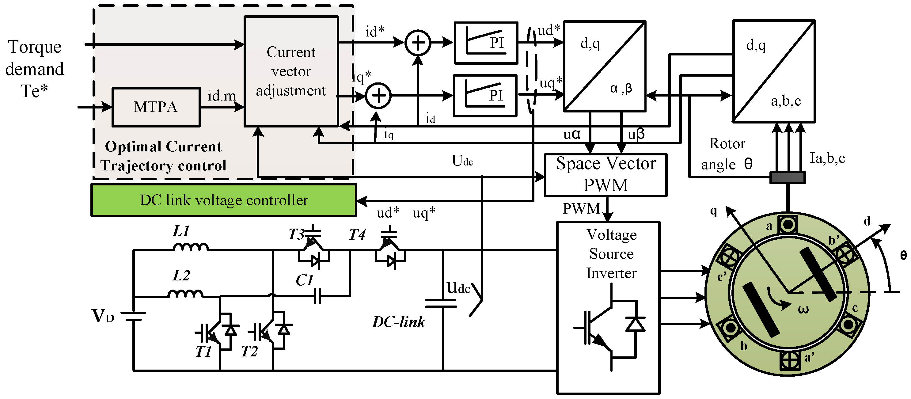
Combining the CTCS, this paper proposes a dynamic DC-link voltage control taking the cross coupling effect and magnetic saturation into consideration. It is a discrete control strategy which takes the asked terminal voltage of the motor as control reference to modify the bus voltage. The purpose of this bus voltage adjustment method is to realize the low DC-link voltage control in low load situation to diminish the system losses and boost the bus voltage in high speed region to delay the flux weakening operation. The arrangement of this paper is as follows: Section 2 introduces the working principle such as the mechanism of the cross saturation effects, the process of dynamic DC-link voltage adjustments. Section 3 displays the details of the simulation tests. A 10 kW IPMSM test rig is set meanwhile, relative experimental works are conducted to validate the accuracy of the strategy. Section 4 presents the conclusions of the paper.
2. Working Principle
2.1. The Cross Saturation Effects
The mathematic model of IPMSM and the electrical restriction boundary of inverters consist of the inductance Ld and Lq, the magnetic flux linkage Ψf, and the stator resistance Rs. Moreover, different control strategies can be traced back to finding a decent current control reference, and the solution procedure is determined by the machine parameters. Therefore, a precise parameter date and its change rules can help to find more accurate control results. Under conventional conditions, the magnetic circuits in the direct-axis (d-axis) and the quadrature-axis (q-axis) are presumed decoupled and the parameters such as flux linkage and inductance are set fixed by default. However, as it shows in Figure 1, the flux linkage in d-axis and q-axis is not completely orthogonal. There has overlapped path between two axis on the stator core which contribute to the mutual inductance Ldq and Lqd. This phenomenon is called the cross coupling effect. By introduce the cross coupling inductance, the flux linkage model can be modified as:
From Equation (1), Ldd and Lqq represent the self-inductances of d-axis and q-axis. Ldq and Lqd are the cross coupling inductances of d-axis and q-axis respectively. Ψf refers to the permanent magnetic flux linkage. id, iq, Ψd, Ψq denote the stator current and flux linkage component in dq coordinates.
Thus, the electromagnetic torque function can be rewritten as:
where Te means the electromagnetic torque. Tecr represents the torque introduced by the cross coupling effect.
In addition, the air gap between rotor and stator of the motor is uneven, and it is mainly distributed on the q-axis; meanwhile the direction of permanent magnetic flux is coincident with the d-axis. It contributes to a lower permeability on the q-axis. Consequently, the amplitude of fluctuation of the flux linkage on q-axis with the stator current is more obvious than it on d-axis. This variation of the flux linkage during the motor operation is called the magnetic saturation effect. In order to evaluate the effect of operating states on the flux linkage and inductance, a 10 kW IPMSM model has been made. Based on the calculation model in [28] the inductance as function of stator current can be derived, however, the model, as Equation (4) displayed, should be modified according to Equation (1) to introduce the cross coupling inductance into account. The finite element analysis (FEA) has been conducted through the ANSYS Maxwell software (15.0.0.).
The results are plotted in Figure 2 and Figure 3. Figure 2 displays the flux linkage varying with dq-axis current, and Figure 3 shows the details of inductances dependent on the armature currents:
Although id plays a predominant role in the d-axis flux linkage, its value slightly increases with iq especially when the demagnetizing current is low, which thanks to the contribution of the cross coupling inductance. The variation range of flux and inductance in q-axis is more significant than in d-axis particularly when the armature current is high. Although the q-axis current determines Lq and Ψq, their value also descends along with the increasing d-axis as shown in Figure 2b and Figure 3b.
According to the discussion above, the inductances are mainly regulated by their own axes current. The mutual interference from another axis current is small down to few millihenry. Therefore, the planar details of inductance variations are computed by the FEA (ANSYS Maxwell 15.0.0) to confirm the specific value. Note that the influence of temperature on inductances and permanent magnetic flux is absent due to the imperfection of experimental instrument. It can be seen in Figure 4, the distinction of Ld is as small as almost 2 mH, in consequence it is deemed to be fixed during the operation. In Figure 4b, the q-axis inductance is dependent on iq, and gives out a nonlinear characteristic. Comparing two results, the difference of the mutual inductance with two axes is negligible, therefore, the mutual inductance is also regarded as constant and equal, that is Ldq = Lqd. These phenomenon are consequent from the cross coupling effect and the magnetic saturation. To simplify the calculation, Lq is linearized as follows:
2.2. Dynamic DC-Link Control Strategy
Figure 5 dislays the overview of the proposed dynamic DC-link voltage control strategy. It can be separated into three parts. First of all, the optimal current trajectory control algorithm converts the torque setpoint into the optimal current reference signal. According to the target current value, the field-oriented control calculates the reference voltage for the generation of the Space Vector Pulse Width Modulation (SVPWM) signal. Then it also initiates the bus voltage adjustment process based on comparing the asked referece voltage and real-time DC-link voltage. By introducing the cross saturation effects, the model of IPMSM is altered. The electromagnetic torque is shiwn by Equation (2). The ternimal voltage needs to be rewritten as:
A bidirectional DC converter is set up to help the DC-bus voltage keeping at a desired value. The DC source voltage amplitude decides the lower bound of the control strategy (Udc,min = 1.5UD), while the upper limit (Udc,up) is limited at 700 V to protect the facilities from voltage overshoot. The inverter applying the space vector PWM control which has its theoretical maximum value, that is:
To discuss the benefits of the dynamic bus voltage, the inverter loss model should be mentioned. Losses of the inverter can be categorized into conduction and switching loss. Based on [29], the conduction loss of half-bridge is as follows:
where, it shows the amplitude of the line current. represents the power factor angle. and are voltage drop of Insulated Gate Bipolar Transistor (IGBT) and Freewheeling diode (FWDI) related to temperature and current which can be described minutely in datasheet. In this paper, VCE = VEC = 24 V. M denotes the modulation index of SVPWM.
The switching loss of IGBT and the reverse recovery loss of FWDI can be derived from Equations (8) and (9):
Eon, Eoff denote the energy loss of IGBT for the turn-on and turn-off process, which are defined by the datasheet. Ts refers to the switching frequency and Err is energy for reverse recovery of FWDI. Udc and Uref represents the bus voltage and the reference DC bus voltage of the IGBT.
The inverter current rating and power capacity is finite, therefore, in order to prevent the system from thermal induced failure and voltage overshoot, the current and voltage of motor should be restricted within a certain range:
It is clear that a lower bus voltage could reduce the switching loss of the inverter. However, the voltage limit of Equation (11) demonstrates that increasing the DC-link voltage could broaden the voltage range, in other words, it could delays the flux weakening operation. Thus, the tradeoff of a proper DC-link voltage according to the operating state could not only enhance the output efficiency, but also extend the speed modulation range. Figure 6 illustrates the schematic process of the proposed DC-link voltage optimization. The bus voltage reference signal can be calculated dependent on the asked voltage reference ud* and uq*, as shown in Equation (12). The bus voltage controller generates the PWM signals to help the DC converter track the voltage setpoint:
where is safety margin to avoid the terminal voltage of IPMSM hitting the limit boundary.
2.2.1. DC-DC Converter Working Principle
The structure of the DC-DC converter is shown in Figure 5. This type of converter can work in two modes, the boost mode and the buck mode. In the boost mode, it energizes the bus voltage based on the control reference. The IGBT of switching devices T1 and T2 and the diode of T3 and T4 participate the conduction process in this mode. In the buck mode, the converter can collect the redundant energy from the load to the DC source and implement the bidirectional function. The IGBT of T3 and T4 and the diode of T1 and T2 play dominant roles in this procedure. In this paper, the DC source UD is fixed and incapable of storing the dumped energy. Therefore the converter is mainly working in the boost mode, but if an energy storage source is applied to the DC source such as a supercapacitor, the converter can realize bidirectional energy flow when the electric vehicles are under special working conditions, for example, during acceleration and regenerative breaking.
When the converter is working at the boost mode, there are a few premises. First, it is assumed to be the continuous conduction mode, CCM. The switching devices use shifting phase parallel control, and the duty cycle should 0.5 < d1 = d2 < 1. The capacitor of the converter is big enough to neglect its voltage ripple. Finally, the inductor currents are continuous. They can be divided into four mode types in one switching period, as shown in Figure 7, where d refers to the duty cycle.
In mode 1, t0 < t < t1, the IGBT in T2 turns on, and the diode of T4 participates in the current flow. The inductance L2 and capacitor C1 provide the electricity for the load. The inductance L1 is charged by the DC source UD, therefore its current could be enlarged as shown in Figure 7d.
In mode 2&4, t1 < t < t2 or t3 < t < t4, the switching device of T1 and T2 are in conducting state, the DC source energizes the inductance L1, L2 and enlarges its current, the voltage of capacitor C1 is in holding state.
In conclusion, the waveform of elements in the converter in each mode can be displayed as Figure 7d. The state equation of the converter in steady state is as follows:
In mode 1:
In modes 2 and 4:
In mode 3:
Based on the inductance “Volt-Second” equilibrium principle, the voltage gain M of the converter working at the boost mode can be derived:
Note that the duty cycle is 0.5 < d < 1, the bus voltage can be enlarged at least four times higher than the DC source voltage applying this type of converter.
2.2.2. Current Vector Adjustment
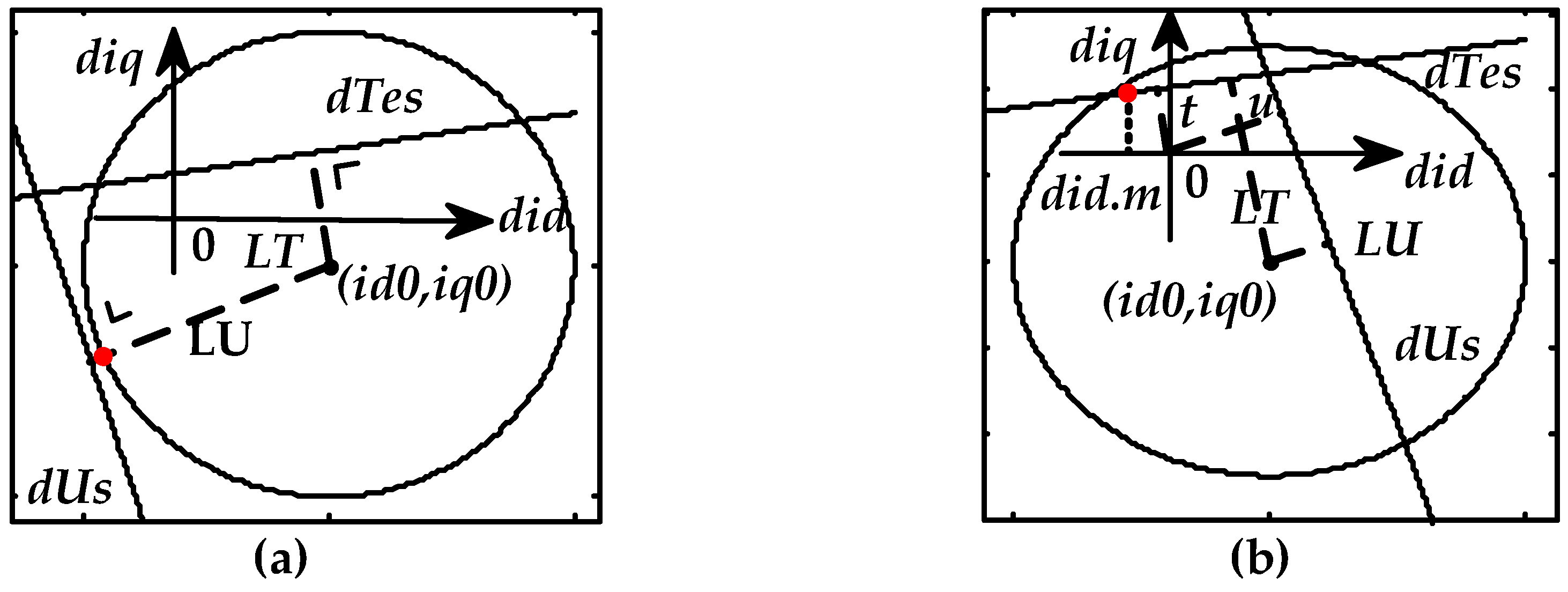
The process details of the current trajectory control strategy (the CTCS) have been analyzed in [27]. As for the safety concerns, the traction drive must operate within the overlapping area of current restrict circle and voltage limit ellipse. These limits could prevent the drive train from breakdown and insulation failure due to overheat and voltage overshoots, especially when they need to be mounted in a confined working space. The CTCS applies a geometrical position method to guide the current vector towards the ideal optimal direction. It takes the parameter variation into consideration and conducts separating among each step. The CTCS operates in the dq-axis incremental coordinate. The torque and terminal voltage has to be discretized consequent to the corresponding position in the current incremental plane. Through the distance between the torque setpoint line and original current vector as shown in Figure 8, the target vector can be derived.
At first, the difference of torque and voltage between target setpoint and the value of the former iteration has to be calculated:
where:
Here ud0, uq0 are the feedback signals of PI controller of former iteration step. Tc is the time constant which is set at 2 ms. Ts is the sample period. From Equations (2) and (6), the current value composed of the torque and the voltage which could be expressed as: y = f(id, iq). The partial differential equation can help to find out the torque and voltage incremental value dependent on current differential signal (did, diq):
It should note that the electromagnetic torque and the terminal voltage model (Equations (2) and (6)) has been adjusted consequent to the cross saturation effects. As it mentioned above, the CTCS conducts in the d-q incremental plane, the differential equation can be regarded as linearized function in these framework:
where:
where:
As shown in Figure 8, the crosspoint of the torque incremental line (Equation (16)) and the voltage modification line (Equation (17)) is the destination for the next iteration. The distance from the original point to the allowed voltage incremental line (LU) is the critical criterion to judge whether it beyond the current limit or not. Due to the overshoot of the voltage can lead some irresistible failure to whore system. Then the length from the origin spot to the target torque incremental line LT is computed:
Although the ideal modification vector is the intersection of torque and voltage incremental line, there is a set of special situations. Firstly, when LU ≥ Imax, the voltage request amount exceeds the radius of the current restricted circle. The vector is the intersection of the current circle and the vertical line which from the origin point to the voltage adjustment line:
Then, if LU < Imax, meanwhile LT ≥ Imax, the modification vector can be calculated through the vertical line from the origin position to the torque request line, the target vector is the crosspoint of the vertical line and the current limit circle:
The results above are needed to judge its position on the voltage incremental line. It must locate at the left hand side of voltage line otherwise the system would loss the control of voltage and extends the error between the result point and the optimal current value idm:
If Dsv < 0, the adjustment vector should be crosspoint of current limit circle and the dUs line:
When the distance between the origin to torque and voltage incremental line are all smaller than the radius of the current limit, the vector can be calculated by introducing the optimal current variation target didm (as shown in Equation (14)):
The criterion Dsv is still available in this circumstance, if the value is negative, the result should be the intersection coordinate of Equations (16) and (17):
Finally, the optimal adjustment vector is derived as follows:
To simplify the resolving process, the flow chart of the CTCS is displayed in Figure 9.
3. Experimental Results and Discussion
This section investigates the influence of the dynamic DC-link voltage control and the cross saturation effects on motor performance. The control strategy is implemented in MATLAB (2010b) SIMULINK. There are three models studied in this paper, namely, Model I which took the entire cross coupling and the saturation effect into account, and it added the DC-link voltage adjustment according to the IPMSM terminal voltage as well. Model II which considered the cross saturation effects, but the DC-link voltage was kept fixed during the test. Model III which neglected the parameter variations and the cross coupling effect, meanwhile, it applied the dynamic DC-link voltage control strategy. The parameters change situation such as the inductance and flux vary with current are shown in Figure 2 and Figure 3. Simulations are conducted using MATLAB/SIUMLINK, but due to this parameter variation, the IPMSM module in the Simulink becomes unavailable so that it should be replaced by the mathematical module. Table 1 provides the specifications of the simulation model and the experimental prototype.
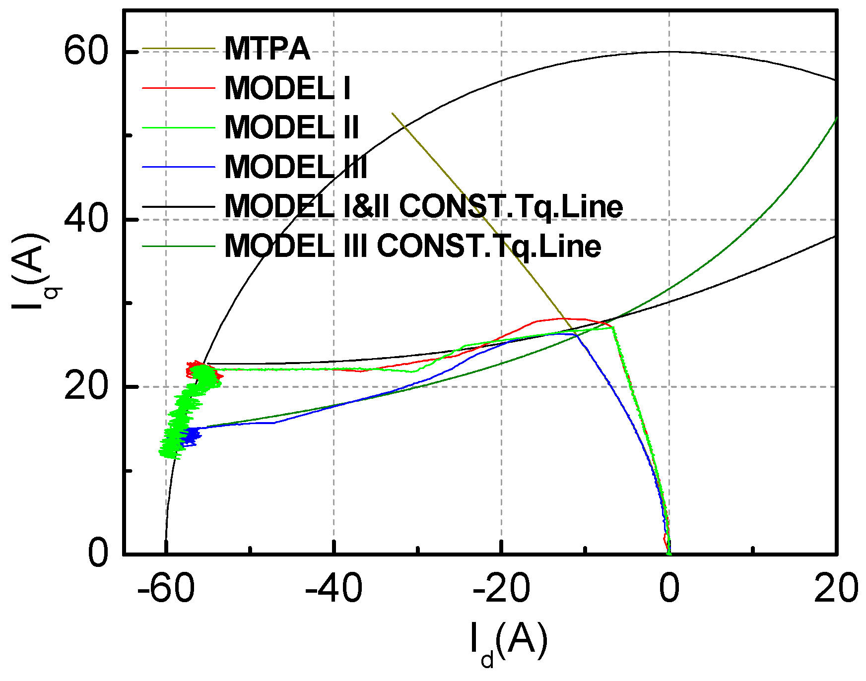
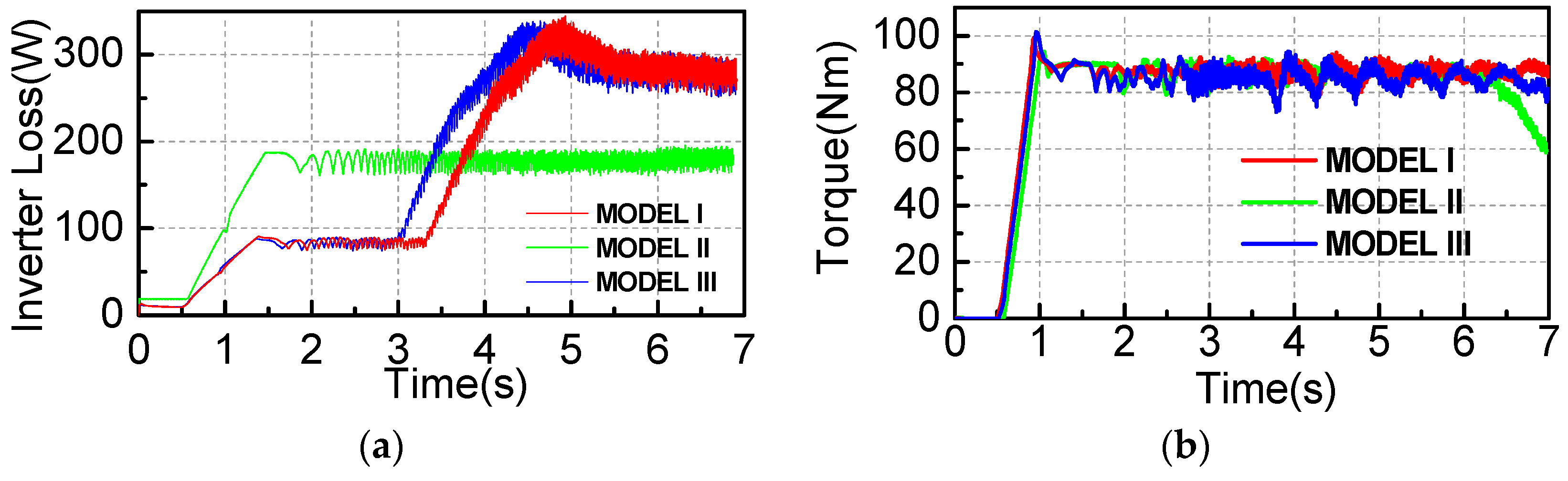
The first simulation was conducted to verify the motor performance at low torque restriction but with a high speed command situation under the proposed dynamic DC-link voltage control. Figure 10 illustrates the current trajectory when the torque is limited to 90 Nm and the motor speed climbs from 0 to 2800 rpm. This restricted torque value is obviously below the theoretical maximum torque, therefore, a decent flux weakening performance is required to deal with the ever-increasing motor speed. As shown in Figure 10, the cross saturation effects can create an upward bias for the constant torque line, it could raise a higher q-axis current component than it in the conventional motor model within the same torque range. Model II is the first to enter the deep flux weakening region. It shows the evidence that enhancing the DC-link voltage in high speed zone can extend the constant torque operation region. Figure 11 shows the DC-link voltage of three models under the proposed DC-link voltage adjustment strategy. Below 750 rpm, the bus voltage of Mode I and Mode III is controlled to the lower limit of 200 V, and the switching loss of inverter can obviously be reduced as shown in Figure 12. Figure 11 also demonstrates that the range of the low DC-link voltage area can be stretched by the cross saturation effects, thus the inverter loss of Model I is smaller than it in Model II. Above 750 rpm, the DC-link voltage grows with the increasing speed, and the discrepancy of inverter loss between Model II and Model I&III becomes smaller. When the speed is higher than 1500 rpm, the bus voltage of Models I and III reaches the top value and remains at 700 V according to the motor terminal voltage, it also means the voltage limit is higher than it in Model II. Therefore the motor could maintain the constant torque drive at high speed without breaking the safety requirement of the voltage limits.
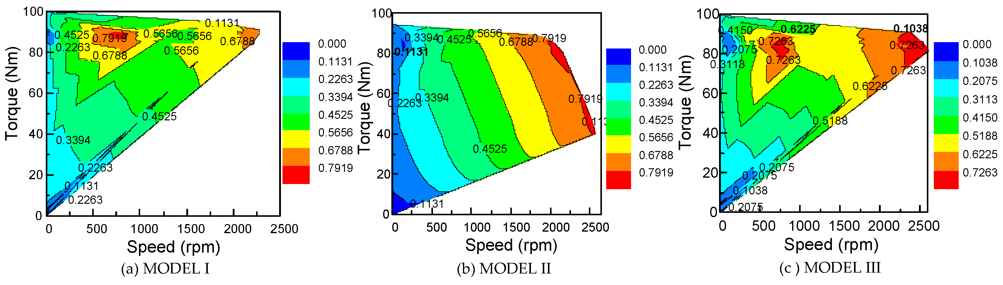
Figure 13 displays the DC-link voltage utilization rate when the torque is limited to 90 Nm. The maximum rates of Model I and Model II are the same. The high utilization area of Model I and Model III is larger than it in Model II. It concentrates on the low speed high torque region and the high speed region which nearly at 2500 rpm, but in Model II, it is just located in the high speed high torque region. The maximum rate of the bus voltage utilization in Model III is the lowest among three models. The utilization rate of the DC-link voltage can be slightly improved by the proposed scheme.
The second simulation was set to demonstrate the influence of the proposed DC-link voltage control strategy taking the cross saturation effects into account under an extreme condition. The torque setpoint was given beyond the maximum value that can be reached, while the speed reference is set to 3000 rpm. As shown in Figure 14, the cross saturation effects have an obvious impact on the MTPA trajectory and the constant torque locus, thus the discrepancy of control strategy applied the fixed parameters will become significant. Figure 15 illustrates that the bus voltage variation trend of Model I and Model III is almost identical in this simulation. Even though the DC-link voltage of Model III is kept at almost 700 V, the terminal voltage still drops gradually because of the saturation effect in q-axis. Figure 12 and Figure 15 are show the evidence that models earn benefits from keeping the bus voltage as low as possible to reduce the inverter loss in low speed region, however, the disadvantage of high loss in high speed area becomes unconsidered in comparison with the advantage of the more extensive constant torque drive area. The difference between torque performances among three models is significant in the second simulation as shown in Figure 16. Note that the slope of Model II and Model III is almost equal, in other words, the turning speed from the constant torque to constant power operation can be increased through boosting the bus voltage, but the range of flux weakening is not changed obviously. However, the slope of Model I is larger than others, the reason is the d-axis current component increases in deep flux weakening operation so that the degree of saturation in q-axis could be relieved which profit from the introduction of the cross coupling inductance.
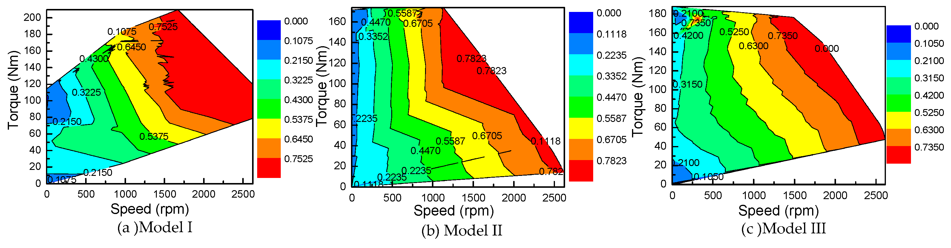
The DC-link voltage utilization rate when the torque is restricted to 190 Nm is as shown in Figure 17. The proposed control strategy helps the system to acquire the largest high voltage utilization rate area among three models. It also can be seen that the top rate value and its area of Model I and Model II are slightly higher than Model III, which indicates that the control strategy considering cross saturation could implement more effective utilization of the dc bus voltage.
From the series of simulation works described above, it can be concluded that the proposed dynamic DC-link voltage adjustment scheme considering the cross saturation effects can expand the motor operation range over the entire speed region, precisely, not only the constant torque region in low speed but also the flux weakening range in high speed, therefore the control precision of algorithm and the motor output characteristic are can be enhanced.
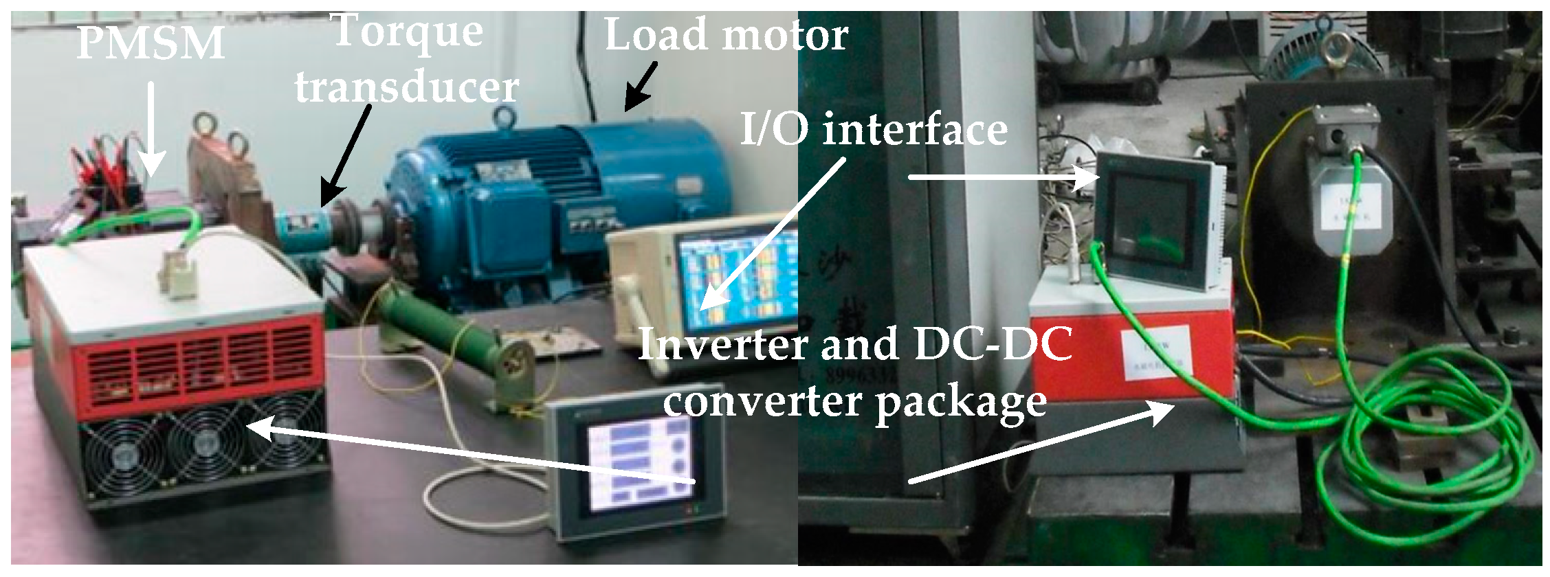
To testify the control strategy, a 10 kW IPMSM prototype has been established, as shown in Figure 18. The 12 kVA active front-end is a DC-DC converter, linked the DC source to realize the modification of the DC-link voltage (it packed with the inverter in the red box in Figure 18). The influence of temperature in the permanent magnet flux was neglected caused by the imperfect facility. The torque was detected by the HNJ-500 torque transducer. The switching and the sampling frequency of the system was 5 kHz. The current transducer is PEM CWT300LF (Power Electronic Measurements Ltd., Nottingham, UK) and the voltage transducer is PINTECH N1070A (PinTech, Guangzhou, China) to acquire the precision signals. There were two groups of experiments under two torque setpoints to show the difference between control strategies, while one model kept the constant DC-link voltage at 450 V.
3.1. Torque Speed Characteristic
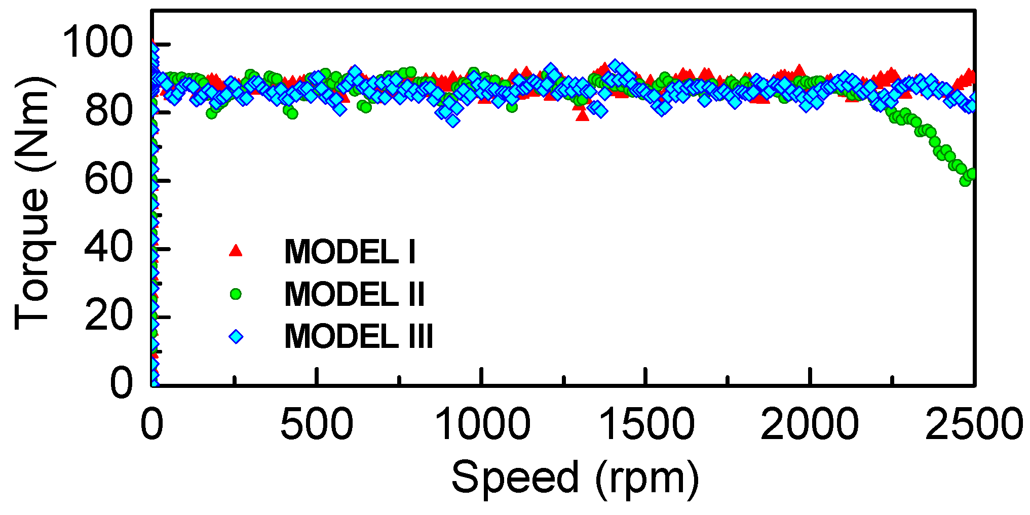
It has been demonstrated elaborately in [27] that the CTCS can help the motor reach its high torque performance potential in low speed region under the low torque setpoint restriction, and in high speed operation, its output torque would be slightly influenced by the magnetic saturation effects. However, in this paper, Figure 19 shows the evidence that the boosted bus voltage can offset the side effect of the cross saturation on the torque performance to delay the flux-weakening operation. As it can be seen, Model II applying the fixed DC-link voltage should sacrifice the torque to ensure the terminal voltage does not exceed the safety boundary.
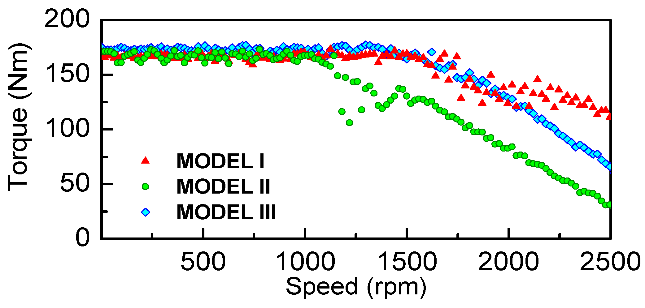
In order to discuss and verify elaborately the influence of the proposed dynamic bus voltage adjustment strategy on the output torque performance, the second test shrinked the current limit and enhanced the torque command value, therefore, it is easier for the motor to enter the flux weakening operation in the process of speed acceleration. Below the turning speed, the achieved torque of Model III is slightly higher than others. Due to the restriction of current trajectory and offset of the MTPA curve, the required demagnetizing current id of Model III is the lowest which could degrade the contribution of the reluctance torque. Despite the small cross coupling inductance and parameter variation, the reflection of torque performance among three control strategies is significant, as shown in Figure 20. The dynamic DC-link voltage control thinking about the cross saturation effect can help the motor dig out its higher potential and earn the wider speed adjustment range is proved.
3.2. Dynamic Performance of Dynamic Voltage Adjustment with Speed Reference Variation
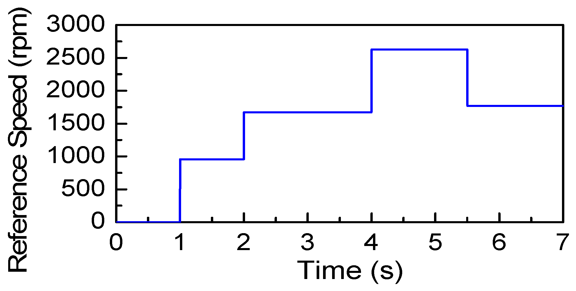
The test prototype is controlled at speed mode. For the first experiment, the reference speed is displayed in Figure 21. The rated speed of the motor is 1500 rpm and the torque value in the control strategy is limited at 90 Nm, which below the theoretical maximum torque. Model I applies the proposed dynamic bus voltage algorithm, while Model II keeps the DC-Link voltage fixed during the test. Both of them seek the parameter variation.
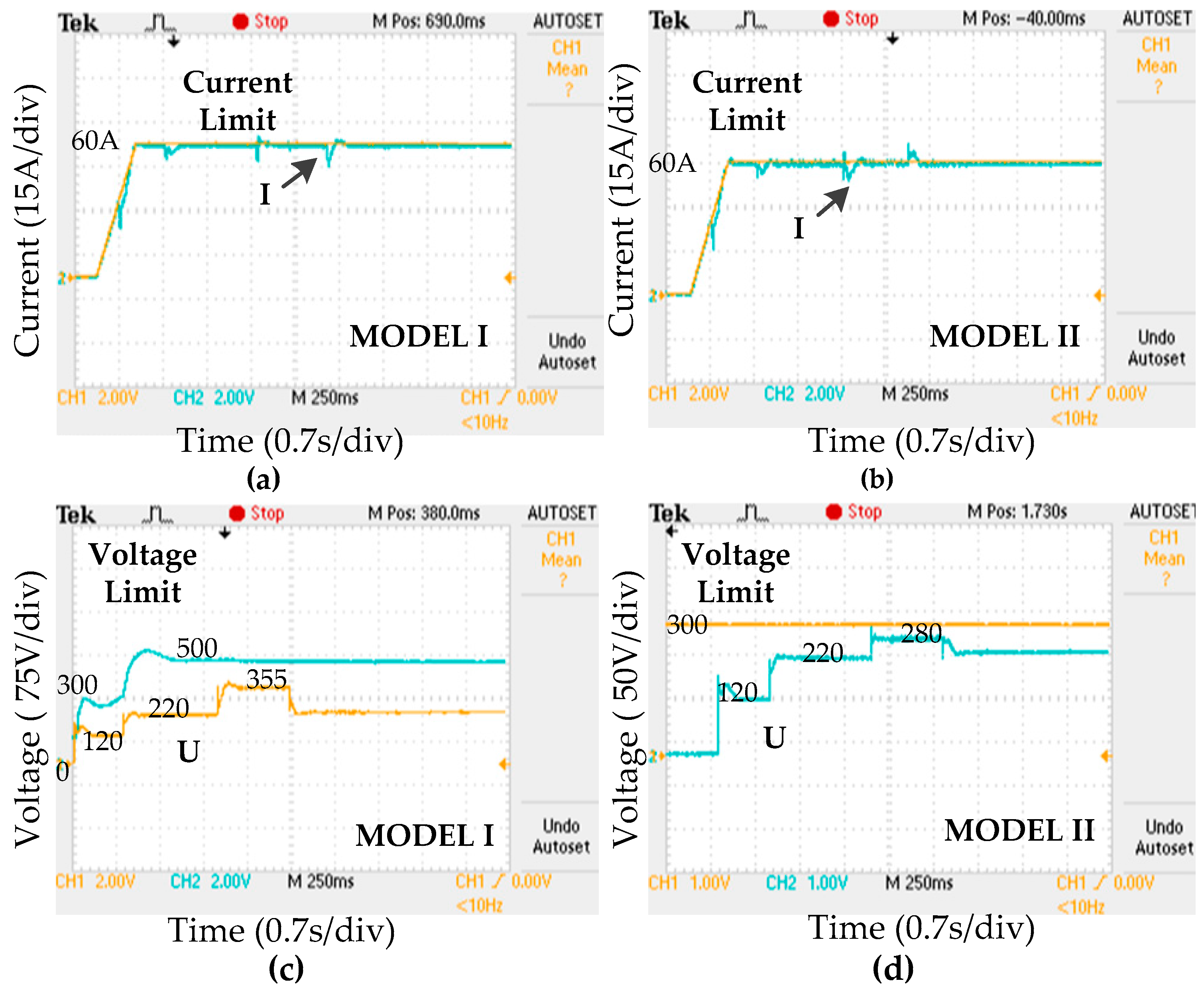
Figure 22 displays the responds of the current and terminal voltage amplitude of the two models. When the reference speed changes, both current and voltage obey the restriction well. The voltage limit of the Model I changes with the step climb of the speed. After 2 s, the speed increases beyond the nominal value, the voltage limit reaches its high boundary near 480 V. The amplitude of terminal voltage are almost the same when the speed is below 2000 rpm, however, after 4 s, the speed reference is stepped to 2500 rpm, the voltage of Model I is higher than that of Model II.
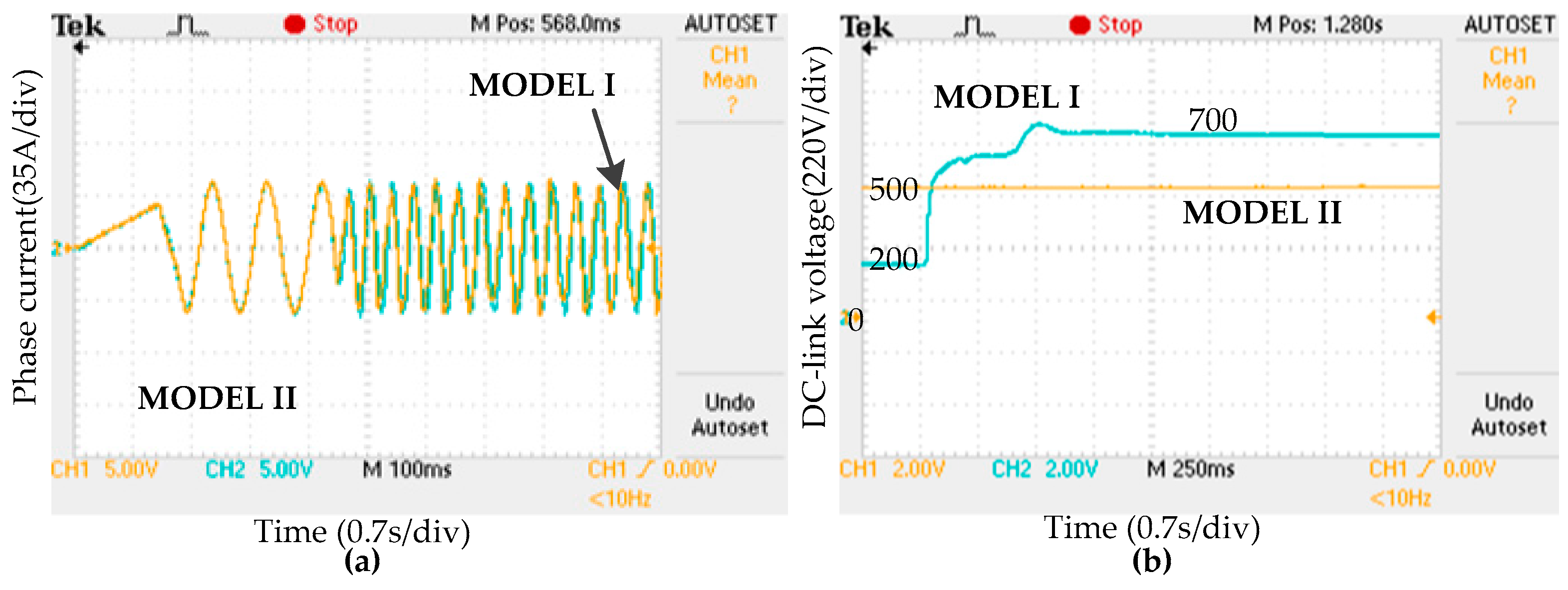
Figure 23 compares the phase current and the bus voltage of the test. The DC-link voltage of the Model II is constant at 450 V. It can be seen that the bus voltage of Model I is lower than the fixed value when the motor speed is below the nominal value. The phase currents of the two models are nearly the same.
In order to discuss the performance of the proposed control strategy when the deeper flux weakening is required, the current limit value is shrunk and the step change amplitude of reference speed is higher than in the first test. Figure 24 reflects the speed reference variation situation.
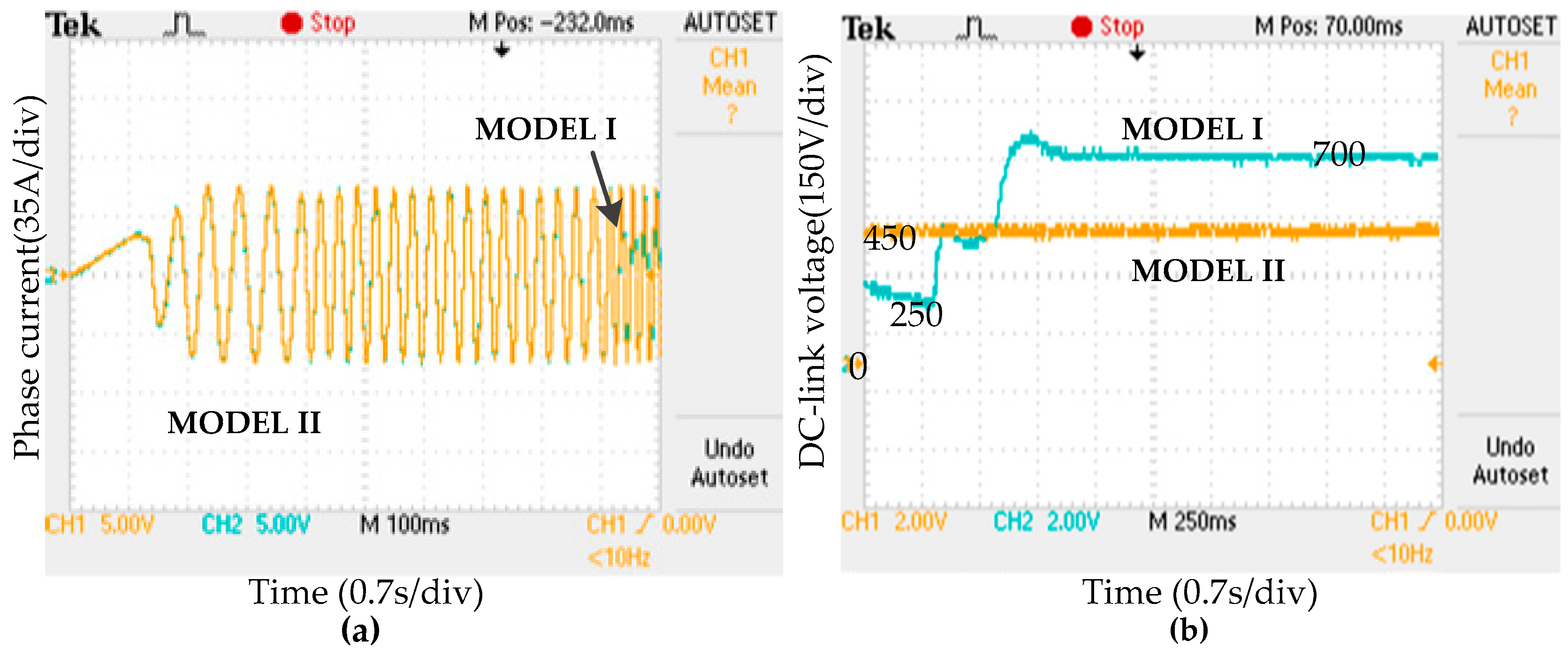
As the current limit shrinks, the turning speed and the theoretical maximum torque value are reduced, therefore, the threshold of the flux weakening control is lower than in the first test. Applying the fixed bus voltage (which is raised to 500 V to protect the test rig), as shown in Figure 25b,d, the fluctuation of the current and the voltage is obviously larger than it in the Model I.
In the low speed area, below 2000 rpm, the voltage amplitude of two models is the same. When the motor accelerates above 2000 rpm, the proposed dynamic DC link voltage control algorithm adjusts the DC-DC converter to boost the bus voltage based on the real-time asked terminal voltage feedback. Note that, despite of the working condition and the torque restriction, the robustness of the control strategy can be observed in these two experiments. The bus voltage in the second test is higher than it in the first test, as shown in Figure 26b. It hits the high boundary at 700 V in high speed region. The phase currant is nearly consistent during the test as shown in Figure 26a.
4. Conclusions
This paper proposes a dynamic DC-link voltage control strategy taking the cross coupling and magnetic saturation effect into consideration. The strategy is divided into three parts: the current reference vector generation, the optimal current vector direction adjustment and the bus voltage regulation. It is a discrete method that could combine and execute variable parameters in each iteration step. The first step translates the torque request into the ideal current reference. Then by estimating the position of linearized torque and voltage line in current incremental coordinates, the optimal current vector can be derived. At last, the bus voltage regulator takes the actual terminal voltage signal as control reference to modify the DC-link voltage. From the simulation and experimental results, the following conclusions can be proposed:
In the low torque command and low speed region, the proposed control strategy is very accurate in tracking the MTPA trajectory without predefined parameters and reduces the inverter loss with low bus voltage. When the speed climbs, the proposed scheme can obviously expand the constant torque operation region, the cross saturation effects have no evident influence on torque performance but it could extend the range of the low DC-link voltage area, which results in a low inverter loss from the global point of view compared with the fixed parameter model.
In the high torque command situation, the range of the whole speed modification area is enlarged by the proposed control strategy, not only the constant torque region but also the flux weakening area. The system stability is guaranteed and the voltage ripple is reduced during the step change of the reference speed.
To sum up: the proposed dynamic DC-link voltage control could not only realize the robustness and high reliability, but also ensures the optimal solution for the globe efficiency. The DC-link voltage utilization can also be improved. In the future, studies will be undertaken in energy feedback and regeneration mechanisms based on the proposed DC-link voltage control scheme by applying supercapacitors or batteries as the DC source with the bidirectional DC-DC converter.
Author Contributions
H.L., D.L. designed the proposed control strategy, H.L. and J.G. conducted experimental works, modeling and FEA simulation, S.H., D.L. and P.F. gave help of paper writing.
Funding
This research received no external funding.
Acknowledgments
This work was supported in part by the Education Ministry Joint Fund of China (51577052).
Conflicts of Interest
The authors declare no conflict of interest.
Nomenclature
| Ld, Lq | d-axis and q-axis inductance |
| Ψd, Ψq | d-axis and q-axis flux linkage |
| Ψf | Permanent magnetic flux linkage |
| Rs | Stator resistance |
| Ldd, Lqq | d-axis and q-axis self-inductance |
| Ldq, Lqd | d-axis and q-axis mutual inductance |
| id, iq | Stator d-axis and q-axis current |
| Ud, Uq | Stator d-axis and q-axis voltage |
| Udc | DC-link voltage |
| φ | Power factor angle |
| VCE, VEC | Voltage drop of IGBT and FWDI base on the datasheet |
| |i| | Amplitude of the line current |
| Eon, Eoff | Energy loss of IGBT for turn-on and turn-off process |
| PCond,igbt, PCond,fwdi | Conduction loss of IGBT and FWDI |
| Psw,igbt, Psw,fwdi | Switching loss of IGBT and FWDI |
| Te | Electromagnetic torque |
| Tecr | Torque introduced by the cross coupling effect |
| Te* | Reference electromagnetic torque |
| Ts | Switching frequency |
| Uref | Reference DC bus voltage of the IGBT |
| Err | Energy for reverse recovery of FWDI. |
| d | Duty cycle |
| UD | DC source voltage |
| M | Voltage gain |
| Δu | Safety margin to avoid the terminal voltage of IPMSM |
| ud0, uq0 | Feedback signals of PI controller of former iteration step |
| Tc | Time constant |
| Imax | Maximum current value |
| LU | Distance from the original point to the allowed voltage incremental line |
| LT | Length from the origin spot to the target torque incremental line |
References
- Amini, M.H.; Islam, A. Allocation of electric vehicles’ parking lots in distribution network. In Proceedings of the 10th Conference on Innovative Smart Grid Technologies (ISGT), Washington, DC, USA, 19–22 February 2014; pp. 1–5. [Google Scholar]
- Zhang, L.; Liu, W.; Liu, Z. A Scope for the Research and Argument Activities on Electric Vehicle Development Mode in Demonstration City. In Proceedings of the 10th Conference on Innovative Smart Grid Technologies (ISGT), Washington, DC, USA, 19–22 February 2014; pp. 394–399. [Google Scholar]
- Zhu, Z.; Lambotharan, S.; Chin, W.H.; Fan, Z. A Stochastic Optimization Approach to Aggregated Electric Vehicles Charging in Smart Grids. In Proceedings of the 10th Conference on Innovative Smart Grid Technologies (ISGT), Washington, DC, USA, 19–22 February 2014; pp. 51–56. [Google Scholar]
- Huynh, T.A.; Hsieh, M.-F. Performance Analysis of Permanent Magnet Motors for Electric Vehicles (EV) Traction Considering Driving Cycles. Energies 2018, 11, 1385. [Google Scholar] [CrossRef]
- Hirschmann, D.; Tissen, D.; Schroder, S.; Doncker, R.D. Reliability prediction for inverters in hybrid electrical vehicles. IEEE Trans. Power Electron. 2007, 22, 2511–2517. [Google Scholar] [CrossRef]
- EL-Refaie, A.M.; Jahns, T.M.; Reddy, P.B.; McKeever, J.W. Modified Vector Control Algorithm for Increasing Partial-Load Efficiency of Fractional-Slot Concentrated-Winding Surface PM Machines. IEEE Trans. Ind. Appl. 2008, 44, 1543–1551. [Google Scholar] [CrossRef]
- Günther, S.; Ulbrich, S.; Hofmann, W. Driving Cycle-Based Design Optimization of Interior Permanent Magnet Synchronous Motor Drives for Electric Vehicle Application. In Proceedings of the International Symposium on Power Electronics, Electrical Drives, Automation and Motion, Ischia, Italy, 18–20 June 2014; pp. 25–30. [Google Scholar]
- Jung, S.-Y.; Hong, J.; Nam, K. Current minimizing torque control of the IPMSM using Ferrari’s method. IEEE Trans. Power Electron. 2013, 28, 5603–5617. [Google Scholar] [CrossRef]
- Morimoto, S.; Takeda, Y.; Hirasa, T.; Taniguchi, K. Expansion of operating limits for permanent magnet motor by current vector control considering inverter capacity. IEEE Trans. Ind. Appl. 1990, 26, 866–871. [Google Scholar] [CrossRef]
- Xu, L.; Zhang, Y.; Guven, M. A New Method to Optimize Q-axis Voltage for Deep Flux Weakening Control of IPM Machines Based on Single Current Regulator. In Proceedings of the 2008 International Conference on Machines and Systems, Wuhan, China, 17–20 October 2008. [Google Scholar]
- Mohamed, Y.R.; Lee, T.K. Adaptive self-tuning MTPA vector controller for IPMSM drive system. IEEE Trans. Energy Convers. 2006, 21, 636–644. [Google Scholar] [CrossRef]
- Consoli, A.; Scelba, G.; Scarcella, G.; Cacciato, M. An Effective Energy-Saving Scalar Control for Industrial IPMSM Drives. IEEE Trans. Ind. Electron. 2013, 60, 3658–3669. [Google Scholar] [CrossRef]
- Sousa, G.C.D.; Bose, B.K.; Cleland, J.G. Fuzzy Logic Based On-Line Efficiency Optimization Control of an Indirect Vector-Controlled Induction Motor Drive. IEEE Trans. Ind. Electron. 1995, 42, 192–198. [Google Scholar] [CrossRef]
- Wang, X.; Xu, S.; Li, C.; Li, X. Field-Weakening Performance Improvement of the Yokeless and Segmented Armature Axial Flux Motor for Electric Vehicles. Energies 2017, 10, 1492. [Google Scholar] [CrossRef]
- Chai, J.-Y.; Liaw, C.M. Development of a switch-reluctance motor drive with PFC front end. Energy Convers. 2009, 24, 271–280. [Google Scholar]
- Lemmens, J.; Driesen, J. Dynamic DC-link Voltage Adaptation for Thermal Management of Traction Drives. In Proceedings of the IEEE Energy Conversion Congress and Exposition, Denver, CO, USA, 15–19 September 2013; pp. 180–187. [Google Scholar]
- Yamamoto, K.; Shinohara, K.; Nagahama, T. Characteristics of permanent magnet synchronous motor driven by PWM inverter with voltage booster. IEEE Trans. Ind. Appl. 2004, 40, 1145–1152. [Google Scholar] [CrossRef]
- Yamamoto, K.; Shinohara, K.; Makishima, H. Comparison between flux weakening and PWM inverter with voltage booster for permanent magnet synchronous motor drive. In Proceedings of the Power Conversion Conference-Osaka 2002, Osaka, Japan, 2–5 April 2002; pp. 161–166. [Google Scholar]
- Sue, S.-M.; Liaw, J.-H.; Huang, Y.-S.; Liao, Y.-H. Design and Implementation of a Dynamic Voltage Boosting Drive for Permanent Magnet Synchronous Motors. In Proceedings of the 2010 International Power Electronics Conference (IPEC), Sapporo, Japan, 21–24 June 2010; pp. 1398–1402. [Google Scholar]
- Okamura, E.S.M.; Sasaki, S. Development of Hybrid Electric Drive System Using a Boost Converter. In Proceedings of the 20th International Electric Vehicle Symposium and Exposition, Long Beach, CA, USA, 15–19 November 2003. [Google Scholar]
- Choudhury, A.; Pillay, P.; Williamson, S.S. DC-Link Voltage Balancing for a Three-Level Electric Vehicle Traction Inverter Using an Innovative Switching Sequence Control Scheme. IEEE J. Emerging Sel. Top. Power Electron. 2014, 2, 296–307. [Google Scholar] [CrossRef]
- Sun, T.; Wang, J.; Chen, X. Maximum Torque Per Ampere (MTPA) Control for Interior Permanent Magnet Synchronous Machine Drives Based on Virtual Signal Injection. IEEE Trans. Power Electron. 2015, 30, 5036–5045. [Google Scholar] [CrossRef]
- Rabiei, A.; Thiringer, T.; Alatalo, M.; Grunditz, E.A. Improved Maximum Torque Per Ampere Algorithm Accounting for Core Saturation, Cross-Coupling Effect, and Temperature for a PMSM Intended for Vehicular Applications. IEEE Trans. Transp. Electrif. 2016, 2, 150–159. [Google Scholar] [CrossRef]
- Li, Z.; Li, H. MTPA control of IPMSM system considering saturation and cross-coupling. In Proceedings of the 15th International Conference on Electrical Machines and Systems (ICEMS), Sapporo, Japan, 21–24 October 2012; pp. 1–5. [Google Scholar]
- Hoang, K.D.; Aorith, H.K.A. Online control of IPMSM drives for traction applications considering machine parameter and inverter nonlinearities. IEEE Trans. Transp. Electrif. 2015, 1, 312–325. [Google Scholar] [CrossRef]
- Lee, S.T.; Burres, T.A.; Tolbert, L.M. Power-factor and torque calculation with consideration of cross saturation of the interior permanent magnet synchronous motor with brushless field excitation. In Proceedings of the IEEE International Electric Machine and Drives Conference, Miami, FL, USA, 3–6 May 2009; pp. 317–322. [Google Scholar]
- Li, H.; Gao, J.; Huang, S.; Fan, P. A Novel Optimal Current Trajectory Control Strategy of IPMSM Considering the cross Saturation Effects. Energies 2017, 10, 1460. [Google Scholar] [CrossRef]
- Chedot, L.; Friedrich, G. A cross saturation model for interior permanent magnet synchronous machine. Application to starter-generator. In Proceedings of the 39th IEEE IAS Annual Meeting, Seattle, WA, USA, 3–7 October 2004; pp. 1–6. [Google Scholar]
- Demetriades, G.; de la Parra, H.; Andersson, E.; Olsson, H. A real-time thermal model of a permanent magnet synchronous motor. IEEE Trans. Power Electron. 2010, 25, 463–474. [Google Scholar] [CrossRef]
Figure 1.
Results of magnet flux circuit with current while the Ψf is set to 0. (a) d-axis flux circuit when iq = 0; (b) q-axis magnet flux circuit when id = 0.
Figure 1.
Results of magnet flux circuit with current while the Ψf is set to 0. (a) d-axis flux circuit when iq = 0; (b) q-axis magnet flux circuit when id = 0.
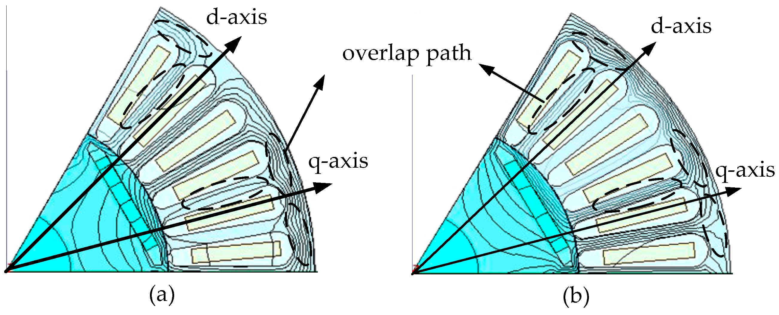
Figure 2.
Flux linkages dependent on dq-axis current. (a) d-axis flux linkage; (b) q-axis flux linkage.
Figure 2.
Flux linkages dependent on dq-axis current. (a) d-axis flux linkage; (b) q-axis flux linkage.

Figure 3.
Nonlinear parameters. (a) d-axis inductance as function of dq-axis current; (b) q-axis inductance as function of dq-axis current.
Figure 3.
Nonlinear parameters. (a) d-axis inductance as function of dq-axis current; (b) q-axis inductance as function of dq-axis current.
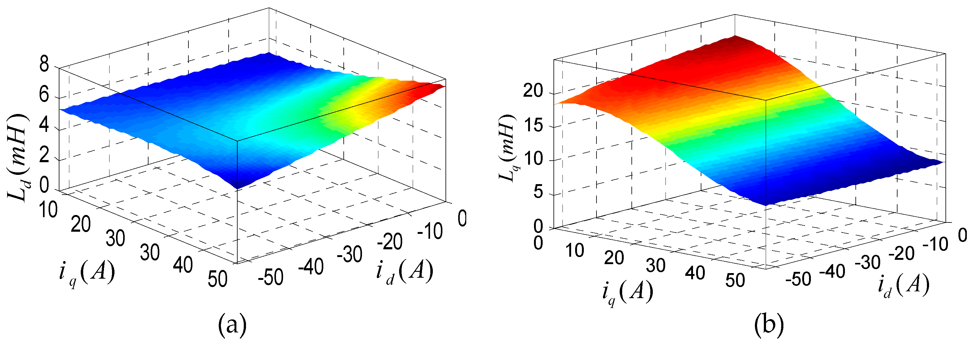
Figure 4.
Inductances as function of its own axis current. (a) d-axis inductance; (b) q-axis inductance.
Figure 4.
Inductances as function of its own axis current. (a) d-axis inductance; (b) q-axis inductance.
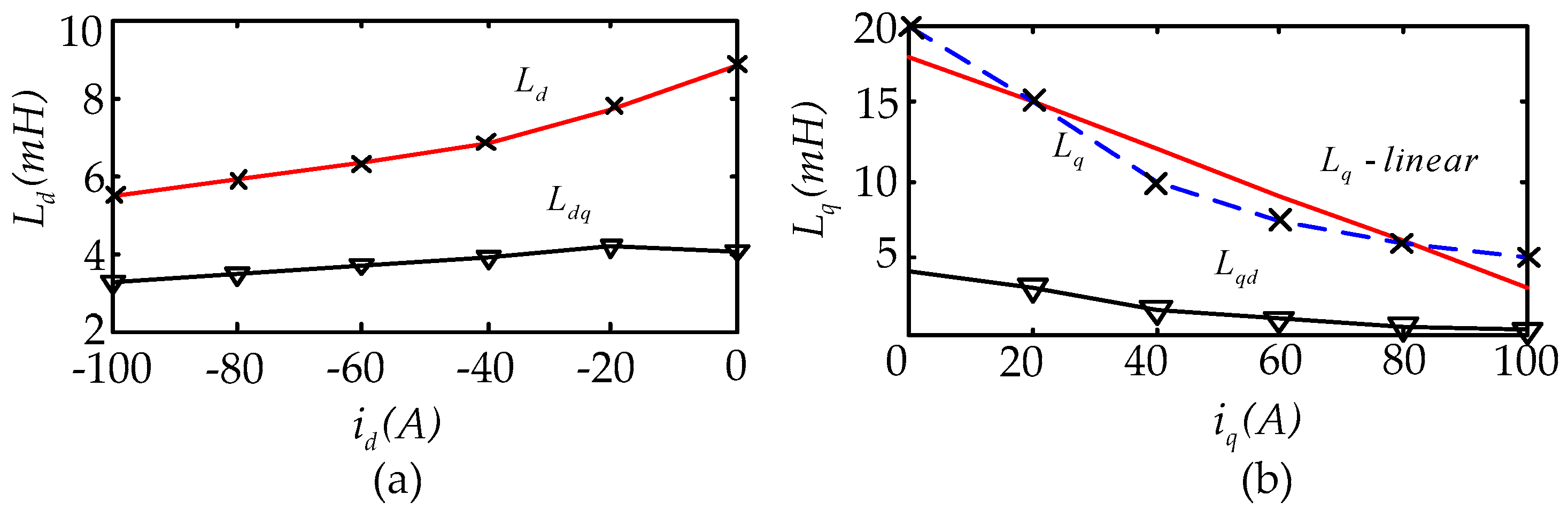
Figure 5.
The overview of the dynamic DC-link voltage control strategy.

Figure 6.
The details of the dynamic DC-link voltage controller.
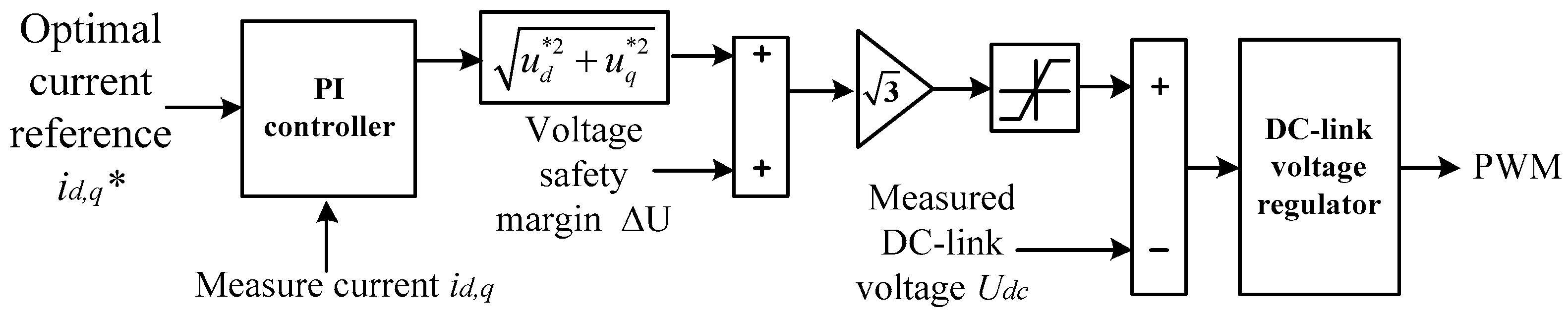
Figure 7.
The working principle of the DC-DC converter: (a) the equivalent circuit of DC-DC converter in mode 1.; (b) the equivalent circuit of DC-DC converter in mode 2&4; (c) the equivalent circuit of DC-DC converter in mode 3; (d) The main waveform of the circuit in the boost mode.
Figure 7.
The working principle of the DC-DC converter: (a) the equivalent circuit of DC-DC converter in mode 1.; (b) the equivalent circuit of DC-DC converter in mode 2&4; (c) the equivalent circuit of DC-DC converter in mode 3; (d) The main waveform of the circuit in the boost mode.
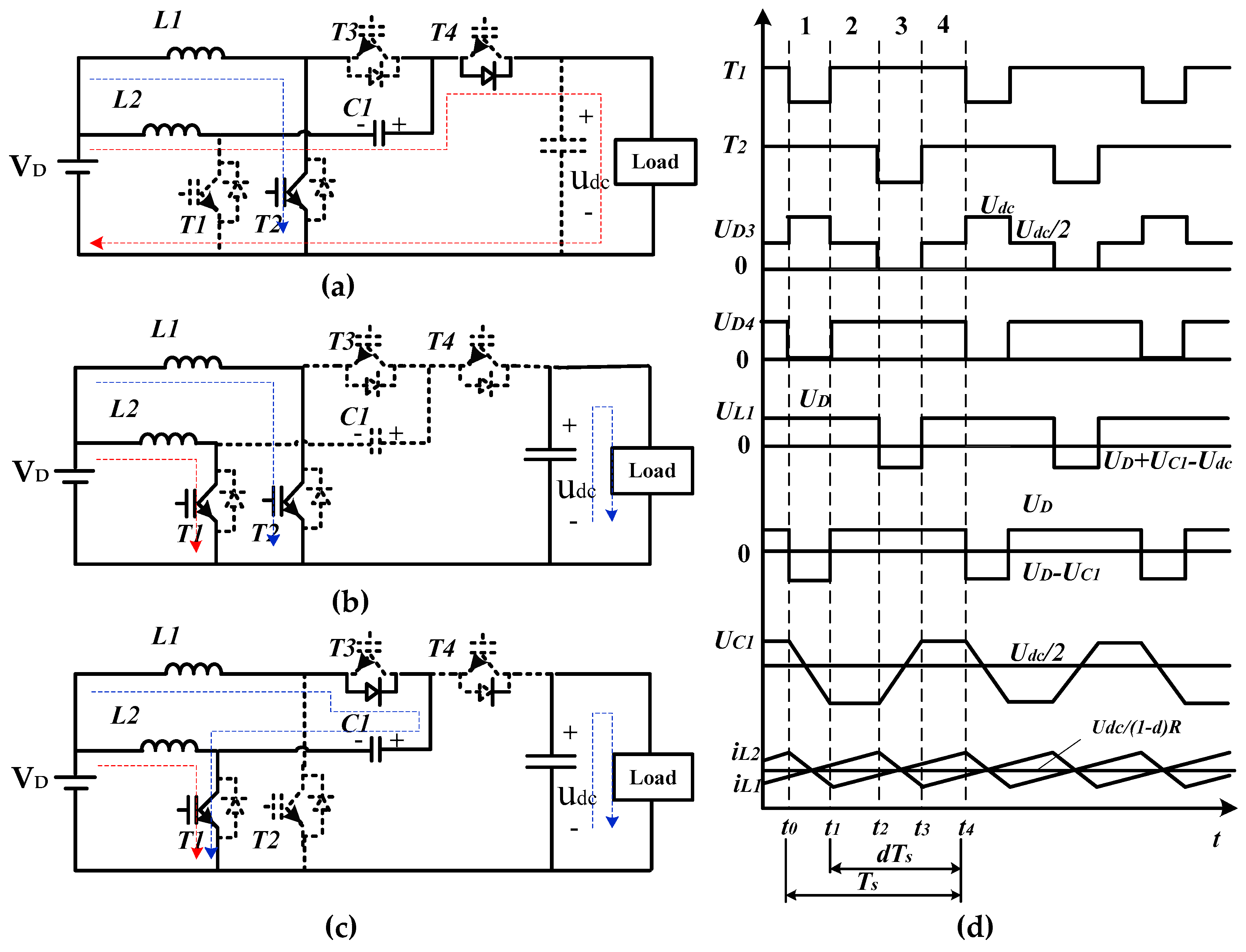
Figure 8.
Graphical illustration of the optimal current vector modification: (a) voltage incremental line in the outside of current circle; (b) The intersection of torque and voltage incremental line in the right hand side of terminal current vector.
Figure 8.
Graphical illustration of the optimal current vector modification: (a) voltage incremental line in the outside of current circle; (b) The intersection of torque and voltage incremental line in the right hand side of terminal current vector.

Figure 9.
Schematic overview of the proposed dynamic DC-link voltage control strategy.
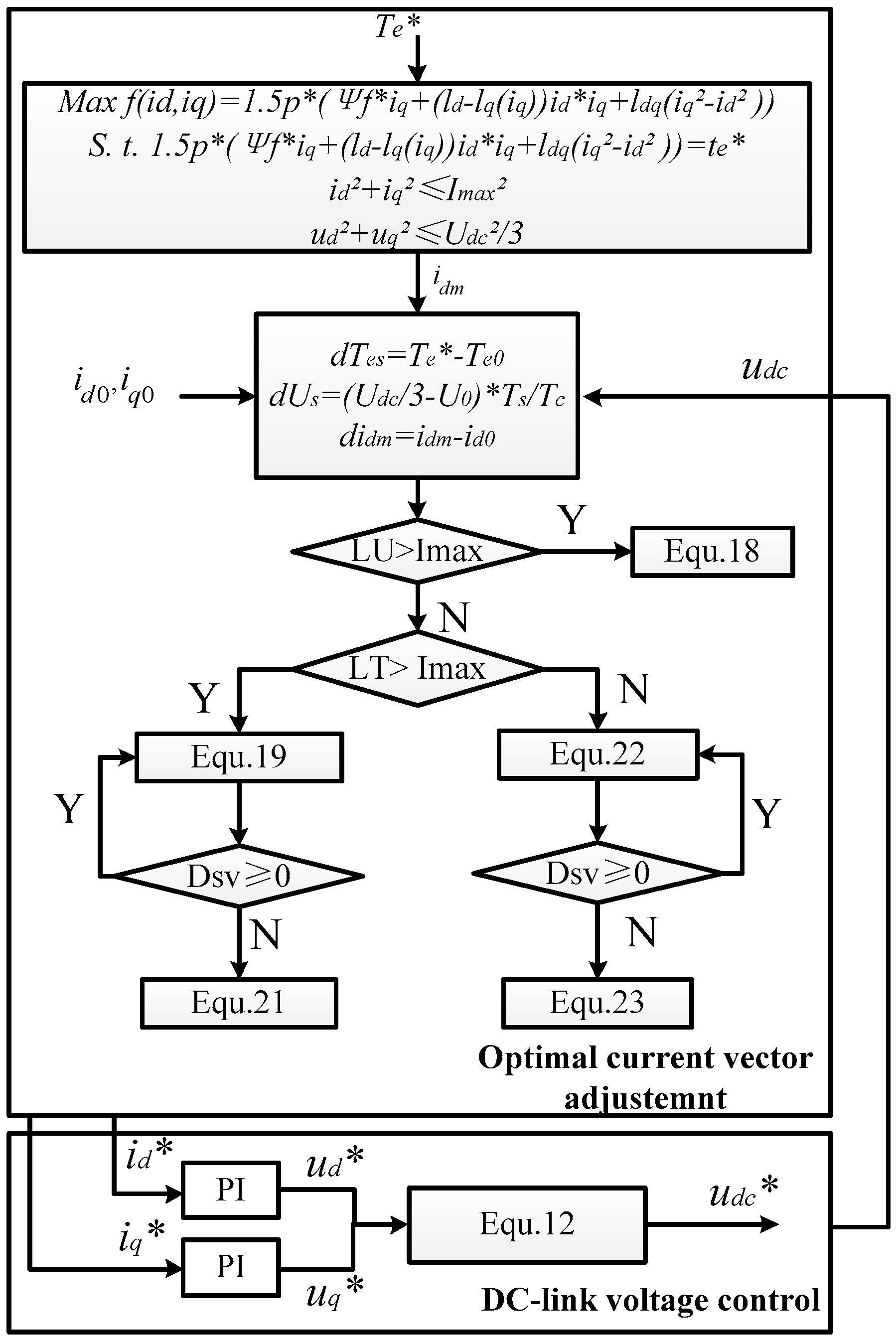
Figure 10.
The current trajectory when torque command is restricted at 90 Nm.

Figure 11.
Simulation results of the bus voltage when torque setpoint is 90 Nm.
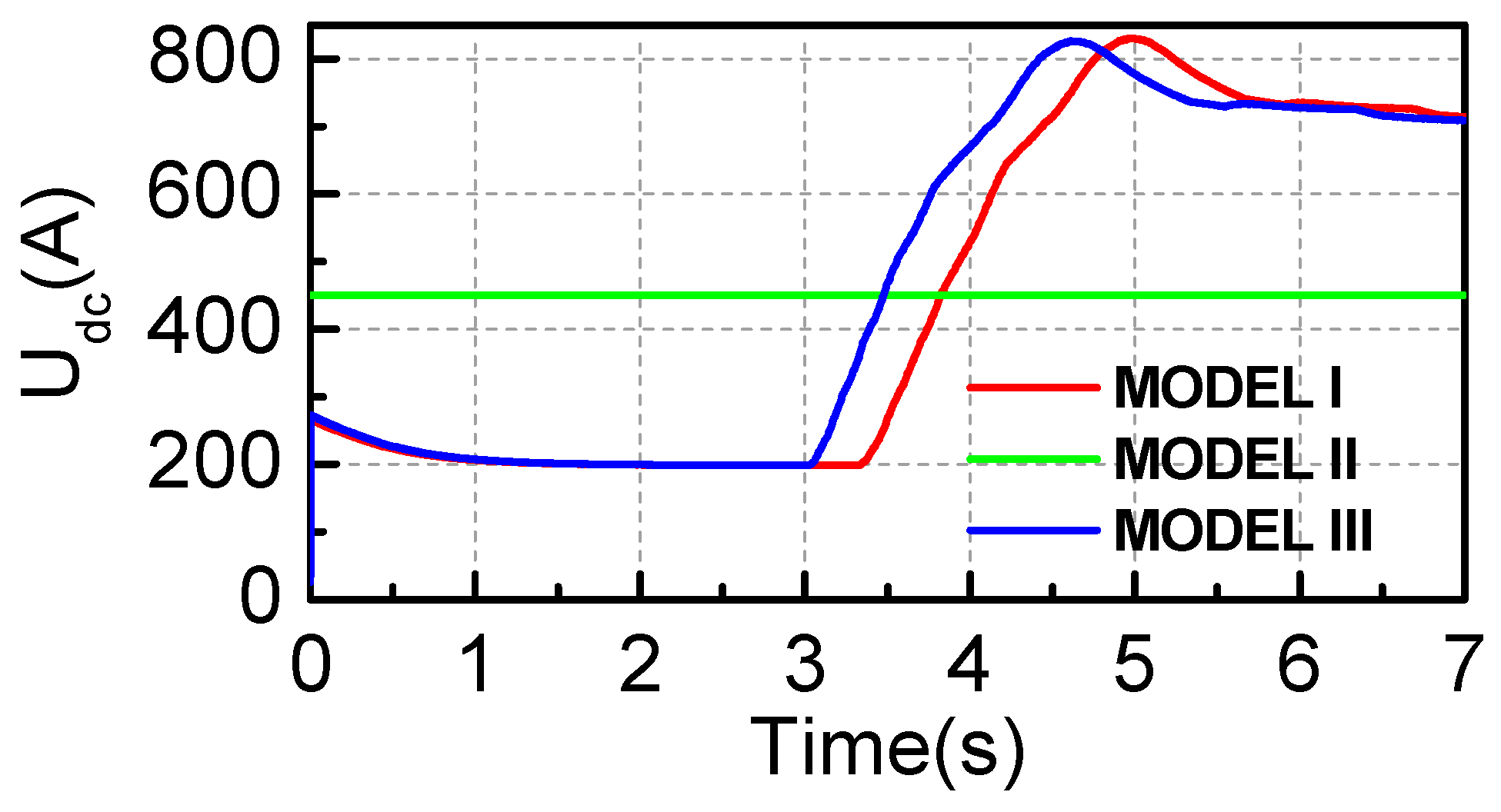
Figure 12.
Simulation results of (a) inverter loss and (b) electromagnetic torque when torque setpoint is 90 Nm.
Figure 12.
Simulation results of (a) inverter loss and (b) electromagnetic torque when torque setpoint is 90 Nm.

Figure 13.
The utilization rate of the dc bus voltage when torque setpoint is 90 Nm.

Figure 14.
The current trajectory when the torque setpoint is 190 Nm.
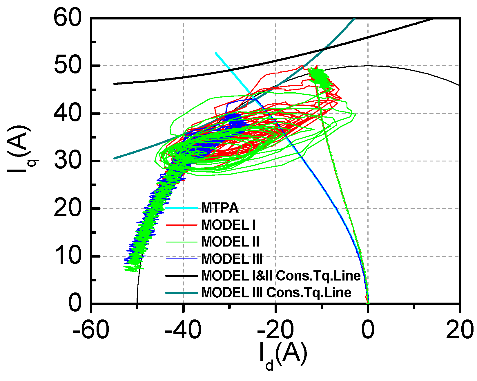
Figure 15.
Simulation result the bus voltage when torque command is limited at 190 Nm.
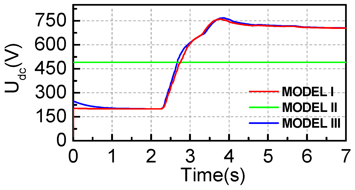
Figure 16.
Simulation result of the (a) inverter loss and (b) electromagnetic torque when torque the command is limited at 190 Nm.
Figure 16.
Simulation result of the (a) inverter loss and (b) electromagnetic torque when torque the command is limited at 190 Nm.
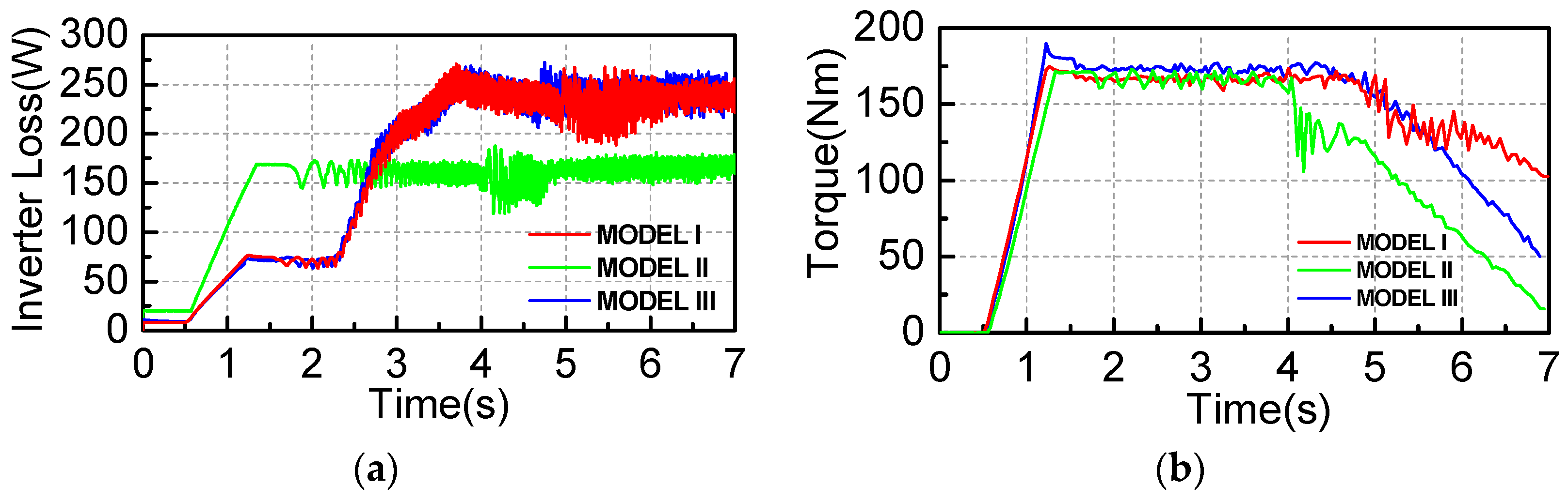
Figure 17.
The DC bus voltage utilization rate when torque the command is limited at 190 Nm.

Figure 18.
Laboratory prototype of current trajectory control with sampling frequency f = 5 kHz.

Figure 19.
Torque-speed characteristic in different models under Te* = 90 Nm.

Figure 20.
Torque-speed characteristic in different models under Te* = 190 Nm.

Figure 21.
The reference speed variation with the DC-link voltage control strategy when torque is limited at 90 Nm.
Figure 21.
The reference speed variation with the DC-link voltage control strategy when torque is limited at 90 Nm.

Figure 22.
Results of current and voltage under the step change of the reference speed when the torque setpoint is 90 Nm. (a) actual current and the current limit of Model I; (b) actual current and the current limit of Model II; (c) actual voltage and the voltage limit of Model I; (d) actual voltage and the voltage limit of Model II.

Figure 23.
The phase current and the bus voltage of two models under Te* = 90 Nm. (a) the phase current; (b)the bus voltage.
Figure 23.
The phase current and the bus voltage of two models under Te* = 90 Nm. (a) the phase current; (b)the bus voltage.

Figure 24.
The reference speed variation with the DC-link voltage control strategy when torque is limited at 190 Nm.
Figure 24.
The reference speed variation with the DC-link voltage control strategy when torque is limited at 190 Nm.
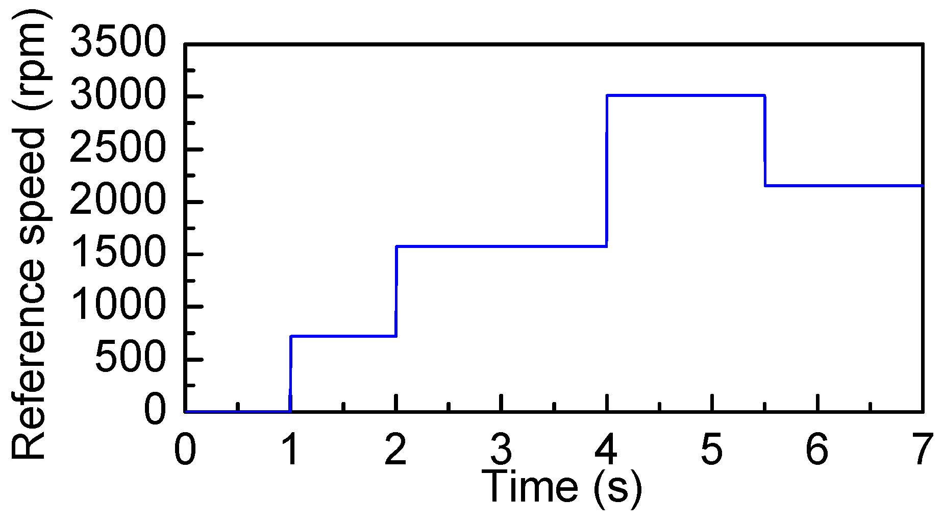
Figure 25.
Response of current and voltage amplitude to the speed reference step variation when torque command is 190 Nm. (a) actual current and the current limit of Model I; (b) actual current and the current limit of Model II; (c) actual voltage and the voltage limit of Model I; (d) actual voltage and the voltage limit of Model II.

Figure 26.
The phase current and the bus voltage value of two models under Te* = 190 Nm. (a) the phase current; (b) the bus voltage.
Figure 26.
The phase current and the bus voltage value of two models under Te* = 190 Nm. (a) the phase current; (b) the bus voltage.

Table 1.
Interior IPMSM specificaation.
| Parameter | Value |
|---|---|
| Rated Power | 10 kW |
| Rated Torque | 70 Nm |
| Rated Speed | 1500 rpm |
| Number of pole pairs | 3 |
| d-axis inductance Ld | 5.6419 mH |
| Mutual inductance Ldq = Lqd | 1.98 mH |
| Stator resistance Rs | 0.03165 Ω |
| Magnetic flux ψf | 0.6304 V·s |
© 2018 by the authors. Licensee MDPI, Basel, Switzerland. This article is an open access article distributed under the terms and conditions of the Creative Commons Attribution (CC BY) license (http://creativecommons.org/licenses/by/4.0/).
Share and Cite
MDPI and ACS Style
Li, H.; Huang, S.; Luo, D.; Gao, J.; Fan, P. Dynamic DC-link Voltage Adjustment for Electric Vehicles Considering the Cross Saturation Effects. Energies 2018, 11, 2046. https://doi.org/10.3390/en11082046
AMA Style
Li H, Huang S, Luo D, Gao J, Fan P. Dynamic DC-link Voltage Adjustment for Electric Vehicles Considering the Cross Saturation Effects. Energies. 2018; 11(8):2046. https://doi.org/10.3390/en11082046
Chicago/Turabian StyleLi, Huimin, Shoudao Huang, Derong Luo, Jian Gao, and Peng Fan. 2018. "Dynamic DC-link Voltage Adjustment for Electric Vehicles Considering the Cross Saturation Effects" Energies 11, no. 8: 2046. https://doi.org/10.3390/en11082046
Note that from the first issue of 2016, this journal uses article numbers instead of page numbers. See further details here.