Stability Analysis of Deadbeat-Direct Torque and Flux Control for Permanent Magnet Synchronous Motor Drives with Respect to Parameter Variations †

Department of electrical engineering, Chonbuk National University, Jeollabuk-do 54896, Korea
†
2013 15th European Conference on Power Electronics and Applications (EPE), Lille, France, 2–6 September 2013.
Energies 2018, 11(8), 2027; https://doi.org/10.3390/en11082027
Submission received: 11 July 2018
/
Revised: 30 July 2018
/
Accepted: 30 July 2018
/
Published: 4 August 2018
(This article belongs to the Special Issue Permanent Magnet Synchronous Machines)
Abstract
:This paper presents a stability analysis and dynamic characteristics investigation of deadbeat-direct torque and flux control (DB-DTFC) of interior permanent magnet synchronous motor (IPMSM) drives with respect to machine parameter variations. Since a DB-DTFC algorithm is developed based on a machine model and parameters, stability with respect to machine parameter variations should be evaluated. Among stability evaluation methods, an eigenvalue (EV) migration is used in this paper because both the stability and dynamic characteristics of a system can be investigated through EV migration. Since an IPMSM drive system is nonlinear, EV migration cannot be directly applied. Therefore, operating point models of DB-DTFC and CVC (current vector control) IPMSM drives are derived to obtain linearized models and to implement EV migration in this paper. Along with DB-DTFC, current vector control (CVC), one of the widely used control algorithms for motor drives, is applied and evaluated at the same operating conditions for performance comparison. For practical analysis, the US06 supplemental federal test procedure (SFTP), one of the dynamic automotive driving cycles, is transformed into torque and speed trajectories and the trajectories are used to investigate the EV migration of DB-DTFC and CVC IPMSM drives. In this paper, the stability and dynamic characteristics of DB-DTFC and CVC IPMSM drives are compared and evaluated through EV migrations with respect to machine parameter variations in simulation and experiment.
1. Introduction
Deadbeat direct torque and flux control (DB-DTFC) was developed by combining the features of deadbeat control and direct torque control (DTC) for induction motor drive systems [1,2]. DB-DTFC has been implemented for various types of electrical machine drives such as IPMSM (interior permanent magnet synchronous motor) drives [3], wound field synchronous machine drives [4], and synchronous reluctance machine drives [5]. Recently, DB-DTFC has been applied for implementation of self-sensing control [6,7] and fault-tolerant control [8]. In [2,3,4,5], it has been presented that DB-DTFC shows advantages over other motor control algorithms, for example, fast dynamic performance and less torque ripple. However, parameter sensitivity is one of the critical issues to be investigated because DB-DTFC algorithm is developed based on an inverse electrical machine model. The parameter sensitivity issue can be reduced by using online parameter identification methods but the methods are typically complicated to implement [9,10,11]. In [12,13], robustness evaluation of DB-DTFC is presented with respect to parameter variations for induction machine (IM) drives and IPMSM drives, respectively. While the torque error, command tracking performance of DB-DTFC for IM, and IPMSM drives have been analyzed, the stability of DB-DTFC with respect to machine parameter variations has not been investigated. In [14], disturbance to a system is estimated using a hybrid Kalman estimator and improvement of robustness is achieved. Not only robustness but also stable operation of motor drives is important, especially for transportation applications, for example, aircraft and electric vehicles.
Though DB-DTFC has shown higher dynamic performance and robustness from previous research, parameter sensitivity is still an important issue to investigate because DB-DTFC is an algorithm developed based on machine model and estimated parameters. In particular, the stability of DB-DTFC with respect to parameter variations should be investigated for practical applications and has not been investigated in other research. Therefore, investigating the stability of a DB-DTFC motor drive with respect to parameter variations is necessary. A few stability evaluation methods for motor drive systems have been presented. The Lyapunov stability theory is applied for stability evaluation of an induction machine drive in [15,16,17]. Using the Lyapunov stability theory, it can be determined if a nonlinear system is (1) Lyapunov stable, (2) asymptotically stable, or (3) exponentially stable. However, the dynamic characteristics of the system are disregarded. In [18], a load angle limiting method is applied to determine a stable region of motor drives. However, the load angle limiting method is torque limitation methods for stable operation of motor drives. A pole-zero migration method is used to investigate stability of motor drives in [19,20,21]. From the pole-zero migration, not only system stability can be investigated but also system dynamic properties, such as frequency of oscillation and rate of decay. Also, the pole-zero migration can be clearly shown in the s-domain and z-domain for analog and digital systems, respectively. Since DB-DTFC is developed based on discrete time model of electrical motors, eigenvalue migration at z-domain is presented in this paper. The eigenvalue migration can be implemented in a linear system while CVC (current vector control) and DB-DTFC IPMSM drives are nonlinear systems. Therefore, deriving linear system models of both IPMSM drives is required. A small signal model or an operating point model is a modeling method used to approximate the dynamics of systems, including nonlinear components, with a linear equation. Using a small signal model of a nonlinear system, the dynamic response and characteristics of the system can be investigated when a small perturbation is applied. Therefore, small signal modeling has been applied for stability analysis of motor control systems and power converters [22,23,24]. In this paper, small signal models of CVC and DB-DTFC IPMSM drives are derived for implementation of EV (eigenvalue) migration.
This paper begins with a brief introduction of a DB-DTFC algorithm and state observers for IPMSM drives. Using the DB-DTFC equation, an operating point model is derived. Then, the eigenvalue migration of DB-DTFC and CVC at z-domain is compared by applying the US06 supplemental federal test procedure (SFTP) driving cycle for practical verification in simulations and experiments.
2. DB-DTFC and State Observers for IPMSM Drives
A DB-DTFC algorithm for IPMSM drives is initially presented in [3]. As stated in Section 1, DB-DTFC shows faster transient dynamics and less torque ripple for various types of electrical machines comparing to other control algorithms but parameter sensitivity is one of the critical issues to be investigated. The DB-DTFC algorithm is briefly introduced in this section because an operating point model is derived based on the DB-DTFC algorithm. Also, state observers used for a DB-DTFC IPMSM drive are reviewed because state observers play an important role in a DB-DTFC system.
2.1. DB-DTFC for IPMSM Drives
Three-phase electrical motors such as PMSMs are typically modeled and analyzed at a rotor reference frame. By utilizing a rotor reference frame, the system complexity becomes simpler than a three-phase model and the direct current (DC)signal can be manipulated for analysis and control instead of alternating current (AC) signals. As shown in Equations (1) and (2), Clarke transformation is applied to transform a three-phase model (a-b-c model) to a stationary reference frame model and Park transformation is applied to transform a stationary reference frame model into a rotor reference frame model.
A graphical representation of the reference frame of a PMSM is shown in Figure 1.
In Equations (1) and (2), subscripts d and q represent the d and q axes and superscripts s and r represent a stationary reference frame and a rotor reference frame, respectively. In (2), θ is the rotor position of a PMSM, as shown in Figure 1. Applying the Clarke and Park transformation, an IPMSM model at a rotor reference frame can be derived. In Equations (3) and (4), differential equations of stator flux linkage, stator current and air-gap torque for IPMSM drives at a rotor reference frame are shown, where p indicates the time differential.
Assuming that the rate of change of torque is constant during the one pulse width modulation (PWM) period (that is, when high switching frequency is applied), the approximate torque difference equation in a discrete time domain is derived as Equation (8) by substituting Equations (3)–(6) into Equation (7). Equations (3)–(6) are presented as a function of stator flux linkages so that the torque equation in Equation (7) does not include stator current vectors when Equations (3)–(6) are substituted into Equation (7).
The Volt-sec solution that results in deadbeat control of IPMSM drives can be obtained as Equation (9) by rearranging Equation (8). It is called the “torque line.”
where, and
This torque line is used in every switching period to solve for the desired inverter volt-seconds that achieve the commanded torque and stator flux linkage [3].
2.2. State Observers for a DB-DTFC IPMSM Drive
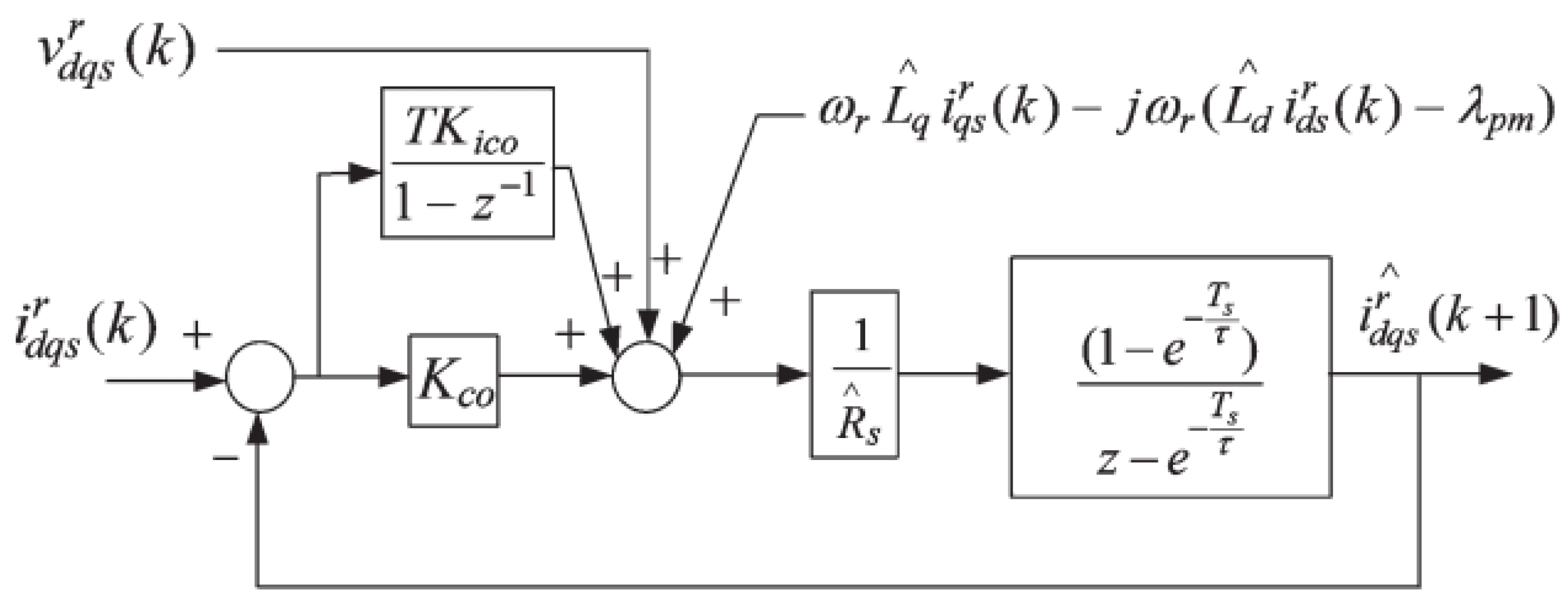
For the development and implementation of a DB-DTFC algorithm for IPMSM drives, a stator current observer and a stator flux linkage observer are required. As a part of the review, a stator current observer and a stator flux linkage observer used for DB-DTFC implementation are briefly introduced in this section. To implement deadbeat direct torque control algorithm, the next sample time instant stator current should be estimated. The estimated stator current is used to calculate the estimated torque and estimated stator flux linkage for the prediction of dynamics one sample time instant ahead [3]. The current at the next sample time instant can be estimated using a rotor reference frame-based stator current observer. The stator current observer is developed based on IPMSM state equations, and its block diagram in a discrete time domain is shown in Figure 2.
The stator current observer is implemented experimentally and its estimation accuracy characteristic with respect to q-axis inductance variation at a frequency domain is presented in [3], as shown in Figure 3.
During the experiment for estimation accuracy, estimated q-axis inductance is detuned ±50% from its correct estimation value to investigate the parameter sensitivity characteristic of a stator current observer of which the bandwidth is 300 Hz. From Figure 3, it is seen that zero steady state error can be achieved within a bandwidth of the stator current observer regardless of parameter variations. Also, the frequency response function shows leading property because the stator current observer estimates the next sample time stator current. A stator flux linkage observer used for DB-DTFC implementation is shown in Figure 4.
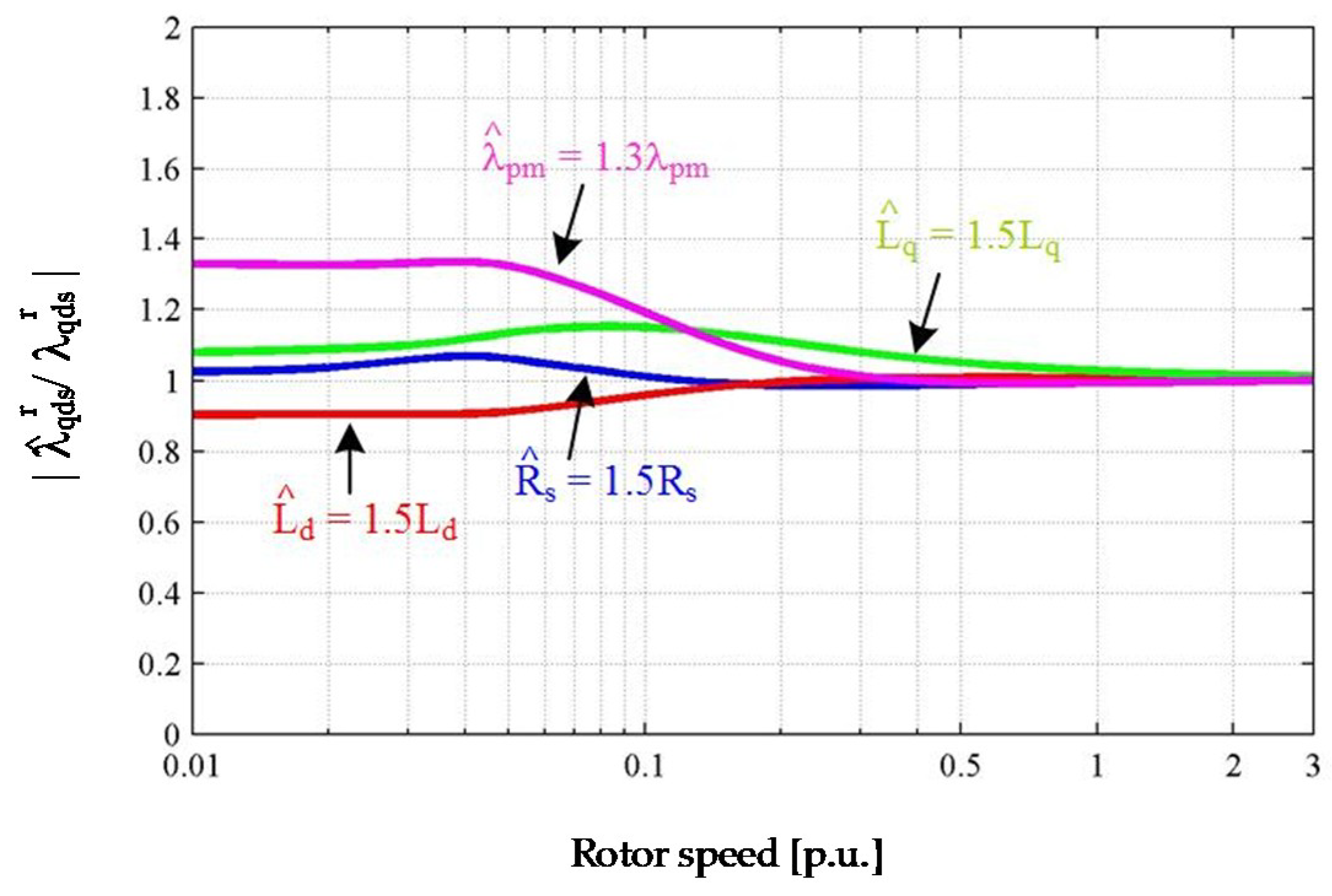
As shown in Figure 4, a current model and a voltage model are used for stator flux linkage estimation of a PMSM. Estimation of stator flux linkage using a current model is not affected by noise signals and dead time but is sensitive to parameter variation. Estimation of stator flux linkage using a voltage model is robust to parameter variations but is affected by voltage distortion such as noise and dead time, especially at low speeds. Therefore, a stator flux linkage is estimated from a current model at low speeds and is estimated from a voltage model at high speed. A cross-over frequency between the current model-based estimation and voltage model estimation is determined by a bandwidth of an observer controller located between a current model and a voltage model. Figure 5 shows the simulation results of a frequency response of the stator flux linkage observer with respect to parameter variations.
As shown in Figure 5, it is verified that accuracy of stator flux linkage estimation is affected by the parameter variations when the operating speed of a PMSM is below a bandwidth of a stator flux linkage observer. Then, stator flux linkage estimation becomes accurate and robust to parameter variation when the operating speed of a PMSM is beyond a crossover frequency of the stator flux linkage observer controller. Characteristics of state observers used in DB-DTFC are reviewed in this section because observers play an important role in a DB-DTFC system and understanding its features and limitation is necessary.
3. Derivation of Operating Point Model of CVC and DB-DTFC IPMSM Drives
3.1. Operating Point Model of IPMSMs
It is known that a nonlinear system behaves similarly to its linearized approximation around an equilibrium point [26]. Therefore, the nonlinear model can be linearized using an operating point model (small signal model). In addition, the stability of a system can be investigated using the operating point model. The operating point models of IPMSM drives can be described by the following equations from [20]:
In Equations (10) to (14), Δ indicates the perturbation of each state, p represents the derivatives of corresponding variables, and o denotes steady state values. The operating point model of IPMSM drives can be formed in a state-space representation. Based on the operating point models in continuous time, Equations (10) through (14), the operating point models in discrete time can be derived as in Equations (15) through (19).
The voltage and current operating point (small signal) model equations, Equations (15) and (16), can be formed in a matrix as in Equation (20):
where
The torque and stator flux linkage operating point (small signal) model equations, Equations (17) and (18), can be formed in a matrix as in Equation (21):
where .
Then, the operating point model between torque and voltage can be written as in Equation (22):
where .
The operating point model, Equation (22), only covers a physical system, i.e., an IPMSM, and its dynamics. Therefore, a controller of an IPMSM is not included in Equation (22). It should be noted that the derived operating point model is sensitive to machine parameter variations such as q-axis inductance saturation with respect to stator current magnitude and permanent magnet flux linkage with respect to temperature. For more accurate modeling, either of the following can be applied as parameters in the operating point model: (1) Look-up table-based parameters varying as a function of operating conditions, or (2) calculated parameters by online estimation method. In this paper, constant parameters are used for analysis. In the following section, operating point models including DB-DTFC and CVC are derived.
3.2. Operating Point Model of DB-DTFC IPMSM Drives
In Figure 6, a block diagram of a DB-DTFC IPMSM drive is shown.
As shown in Figure 6, torque and stator flux linkage commands, estimated torque and estimated stator flux linkage are input signals of the DB-DTFC algorithm block. For efficient operation of a DB-DTFC IPMSM drive, pre-calculated copper loss minimizing stator flux linkage is selected from a maximum torque per ampere (MTPA) look-up table as stator flux linkage command. For estimation of torque and stator flux linkage, a stator current observer and a stator flux linkage observer are used in a DB-DTFC IPMSM drive. Block diagrams of observers can be found in Figure 2 and Figure 4.
In this section, an operating point model (or a small signal model) of a DB-DTFC IPMSM drive is derived. Since DB-DTFC is a model inverse solution, a closed-loop system including DB-DTFC can be written as in Equation (23):
A transfer function of a closed loop DB-DTFC system can be derived as in Equation (24) by expanding Equation (23):
If the estimated machine parameters match the actual machine parameters, that is, A = , B = , C = , and D = , the transfer function becomes deadbeat as in Equation (25):
If estimated parameters do not match the actual machine parameters, the characteristic equation, the denominator of the transfer function of the closed loop DB-DTFC system becomes Equation (26):
The roots of the characteristic equations are the eigenvalues (EVs) of the closed loop DB-DTFC system. The EV migration on a z-plane shows properties of IPMSM dynamics, such as stability, response time, and oscillation.
3.3. Operating Point Model of CVC IPMSM Drives
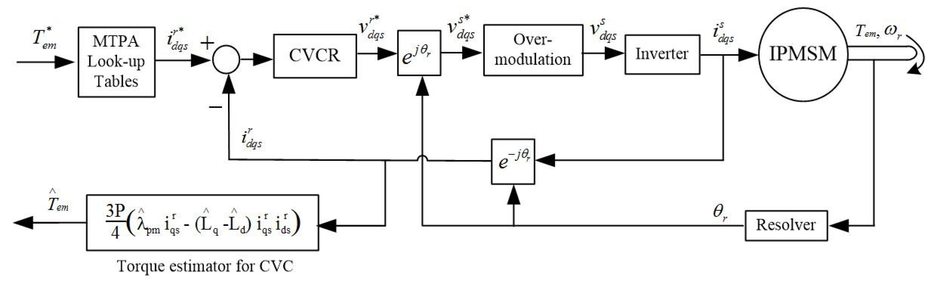
A block diagram of a current vector controlled (CVC) IPMSM drive is seen in Figure 7.
For CVC, a closed loop system including PI controllers can be derived as in Equations (27) and (28):
The operating point model equations of the closed loop CVC system can be written as in Equations (29) and (30):
By substituting Equation (19) into Equations (29) and (30), Equations (29) and (30) become functions of and , as shown in Equations (31) and (32):
Equations (31) and (32) can be written in a matrix form as in Equation (33):
where
The operating point (small signal) models for the DB-DTFC and CVC IPMSM drives are derived in Equations (26) and (33), respectively. Using the operating point (small signal) models, the EV migration of each motor drive is analyzed in simulations and experiments.
4. Simulation Results
Since most driving cycles cover a wide operating space of a motor drive, a driving cycle is chosen as the load and command trajectories for a stability evaluation of DB-DTFC and CVC IPMSM drives. Among automotive driving cycles, the US06 SFTP automotive driving cycle is selected as a stability test trajectory in this paper because it contains high acceleration conditions, which are more suitable for dynamic operation testing of a motor drive. Torque command trajectory for US06 SFTP is developed by multiplying traction force and wheel radius of a test vehicle as in Equation (34), where Ttr is the traction torque, Ftr is the fraction force, and Rwh is the wheel radius of a test vehicle:
Equation (35) is an equation to calculate traction force; Km is the rotational inertia, mv is the mass of a test vehicle in kg, av is the acceleration of a test vehicle, and Fdrag is the drag force. The drag force in Equation (35) can be calculated using Equation (36):
In Equation (36), Dair is air density and Cd is the aerodynamic parameter, which is typically 0.2~0.4. Af is the front area of a test vehicle and vx is the velocity of a test vehicle in meters per second. For more accurate torque trajectory development, additional forces such as rolling resistance force can be applied. Since the actual speed and torque trajectories of the US06 driving cycle cannot be applied directly, the trajectories are adjusted to fit to the rated capacity of the test IPMSM. Time range and scale are also changed so that the data size of the simulation results does not exceed the memory capacity of a computer.
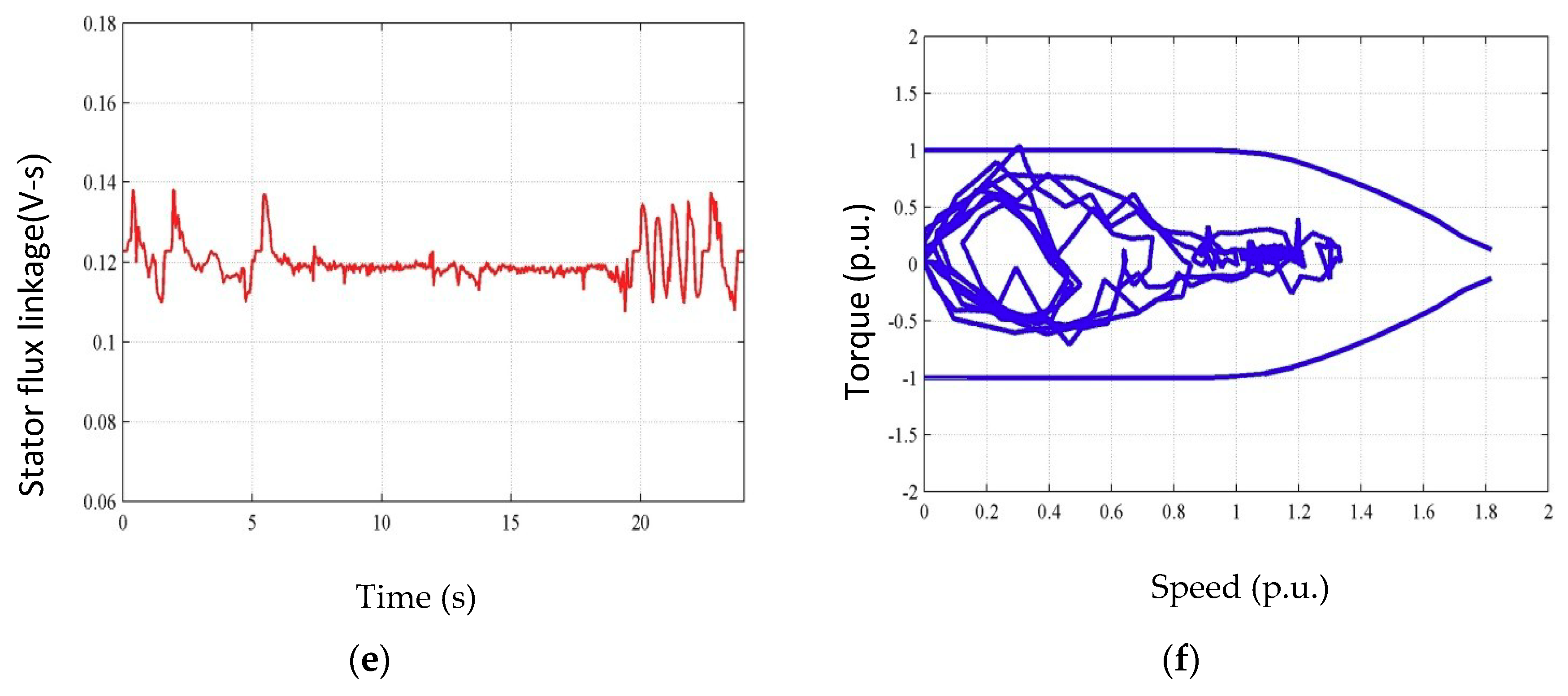
The simulation results for the US06 SFTP automotive driving cycle using DB-DTFC and CVC are shown in Figure 8. Since simulation results using both control algorithms are the same, the results are overlaid. As shown in the simulation results, the operating speed range is increased over the rated speed (Figure 8b), including flux weakening operation (Figure 8e,f), and the torque trajectory of the driving cycle covers up to the rated torque of the test IPMSM (Figure 8a). In addition to operation within a rated operating condition, operation at voltage and current limits (Figure 8c,d) is also investigated when the test IPMSM is driven along the US06 automotive driving cycle. Since the MTPA look-up tables applied for DB-DTFC and CVC shown in Figure 6 and Figure 7 are developed using identical parameters and conditions, the d and q axis current vectors are the same for both control methods. For implementation of DB-DTFC, stator flux linkage and stator current observers are required. Therefore, the complexity and computational effort are higher than in CVC. From the simulation results in Figure 8, the advantages of DB-DTFC over CVC are not directly shown. Though the US06 SFTP is one representative dynamic driving cycle, the corresponding speed and torque trajectories are relatively smooth to present the performance difference between the CVC and DB-DTFC algorithms. A comparison of the CVC and DB-DTFC algorithms based on the simulation results is given in Table 1.
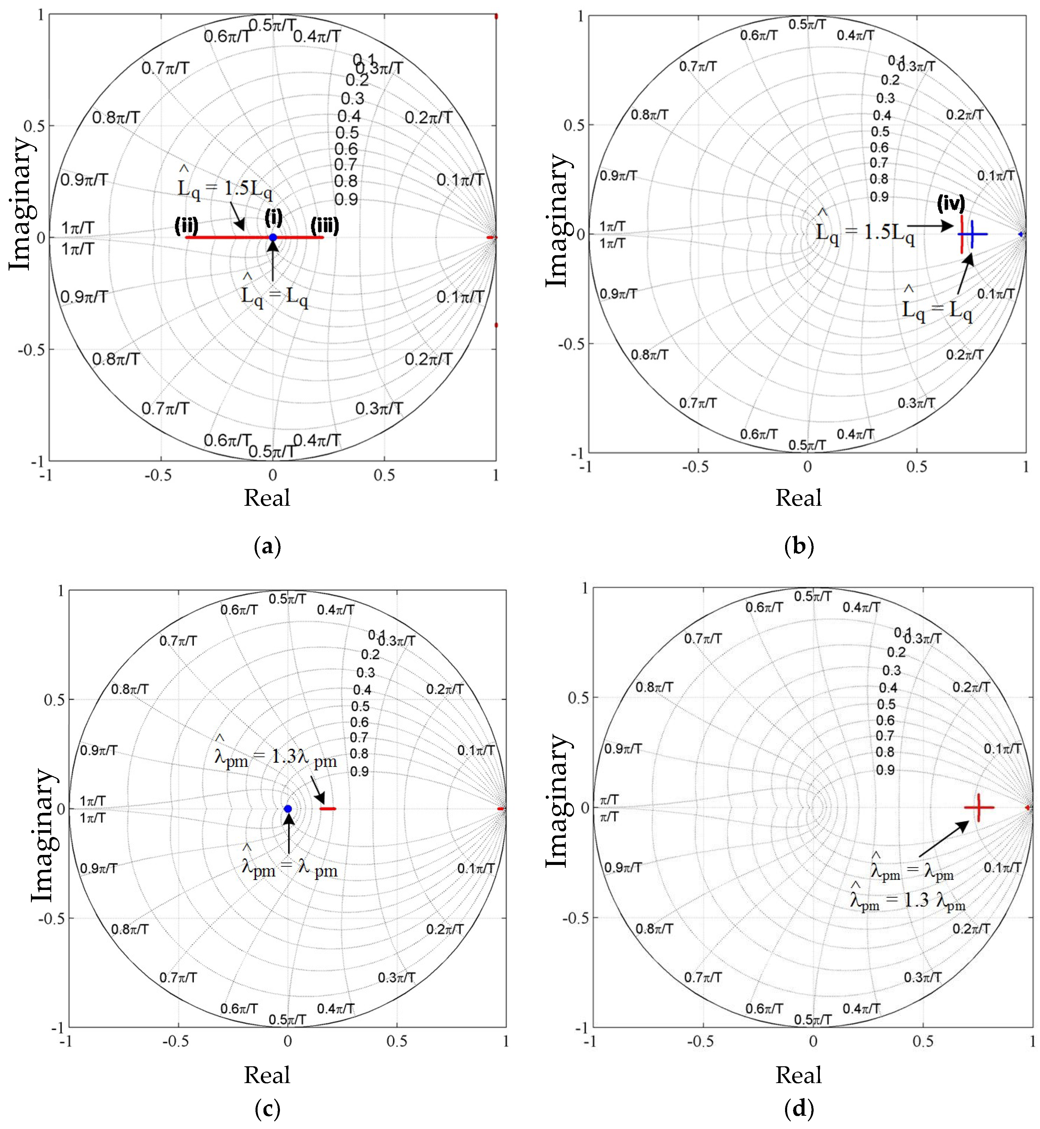
In addition to analyzing CVC and DB-DTFC using time domain simulation results, the EV migration of CVC and DB-DTFC is compared at different points. Utilizing data from the simulation results in Figure 8 and the derived operating point (small signal) models of DB-DTFC and CVC IPMSM drives, the EV migration of each system can be investigated as shown in Figure 9. To investigate the EV migration characteristics of the CVC and DB-DTFC IPMSM drive systems with respect to machine parameter variations, q-axis inductance is detuned by 50% of its actual value intentionally, as shown in Figure 9a,b, and permanent magnetic flux linkage is also detuned by 30% of its actual value, as shown in Figure 9c,d. In the case of a DB-DTFC IPMSM drive, poles are always located at the center of a z-plane, as seen in Figure 9a,c, if the estimated parameters used for the DB-DTFC algorithm exactly match the actual electrical machine parameters. This means that the deadbeat response is achieved along the torque and speed trajectories. If the parameters in the DB-DTFC and the machine parameters are different, the poles move away from a center of a z-plane, as seen in the red trajectories in Figure 9a,c. As a pole moves away from the center of a z-plane, the dynamic response becomes slower, which means that deadbeat response is not achieved any more. Though deadbeat response is not achieved when machine parameters do not match, faster dynamic response can still be achieved using DB-DTFC than CVC. In the case of a CVC IPMSM drive, poles are located and move around near the bandwidth of the current vector controller, as shown in Figure 9a,c. The location of poles is changed as shown in Figure 9b when detuned q-axis inductance is used because inductance is used for calculation of controller gains of a current vector controller.
Since 50% higher q-axis inductance is used for controller gain calculation, the bandwidth of the controller becomes higher and a faster dynamic response is achieved than the desired dynamic response shown in Figure 9b. Unlike q-axis inductance variation, a change in the permanent magnet flux linkage does not affect the dynamic characteristics, as shown in Figure 9d, because permanent magnet flux linkage is not used for controller gain tuning. As seen in the simulation results in Figure 9, eigenvalues are located within the unit circle in the z-plane for both the CVC and the DB-DTFC IPMSM drives. This means that the operation of both motor drive systems is stable along the US06 automotive driving cycle regardless of the machine parameter variations. Figure 10 shows corresponding impulse responses with respect to EV locations of the DB-DTFC and CVC IPMSM drives specified in Figure 9.
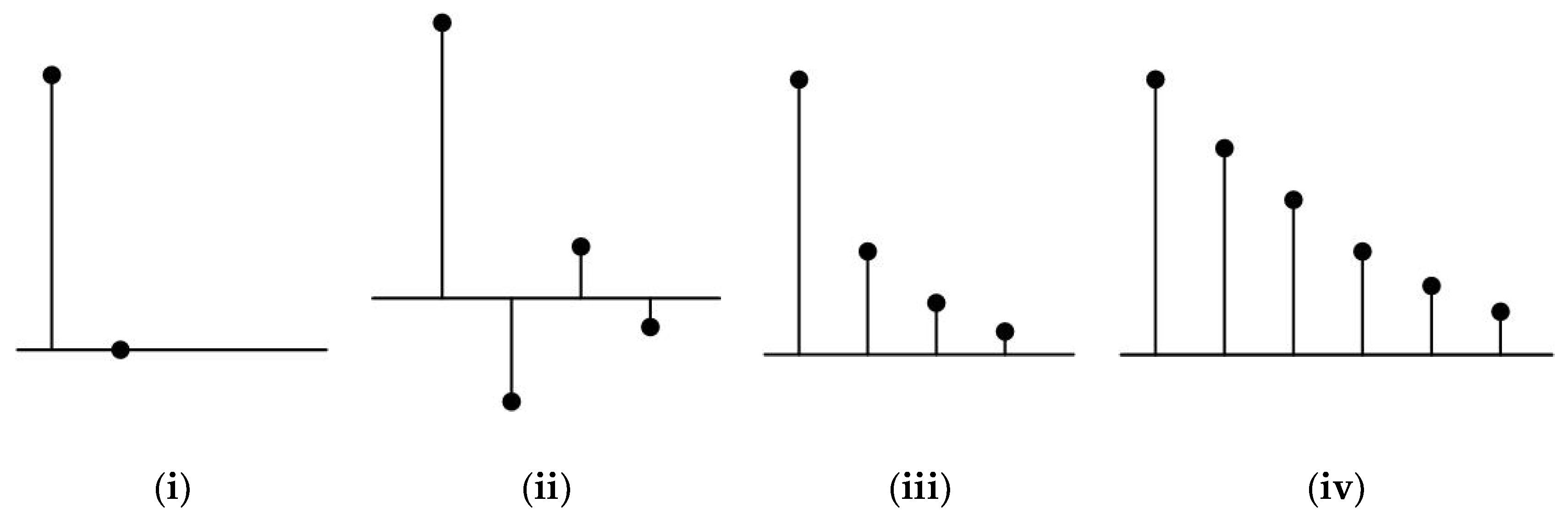
As shown in Figure 10a, deadbeat response can be achieved when an accurately estimated parameter is used for the implementation of DB-DTFC. However, DB-DTFC sometimes results in forced oscillations, as seen in Figure 10b, or a deadbeat response is not achieved, as seen in Figure 10c, when an inaccurate machine parameter is used for the implementation of DB-DTFC. Though forced oscillation occurs, the oscillation does not continue for a long time. This means that the dynamic performance of DB-DTFC is still faster than that of CVC, regardless of the forced oscillation.
5. Experimental Results
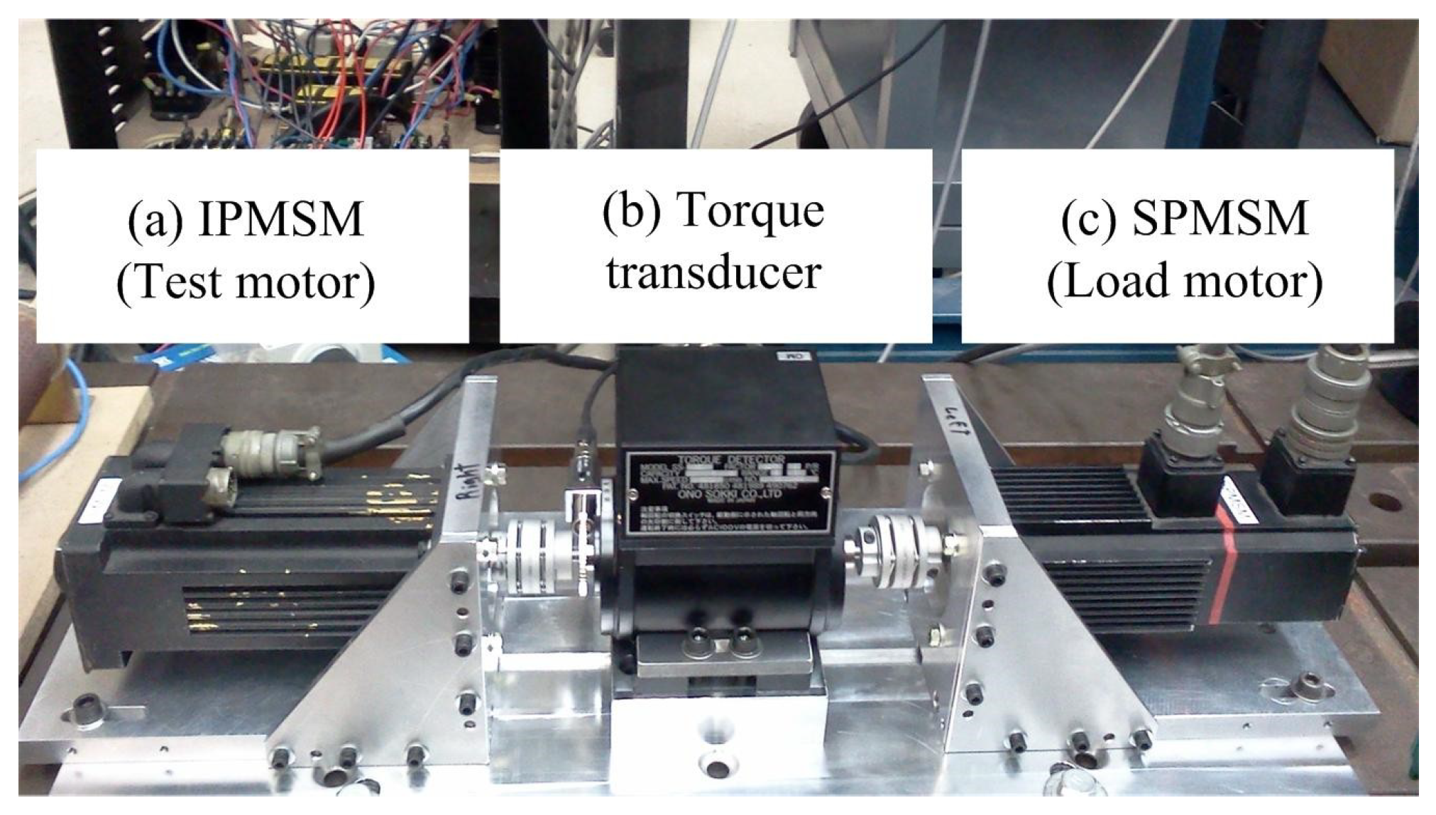
Following simulation, the eigenvalue migration of DB-DTFC and CVC IPMSM drives is implemented and verified experimentally. The experimental test set-up is shown in Figure 11 and the specifications of the test IPMSM are summarized in Table 2.
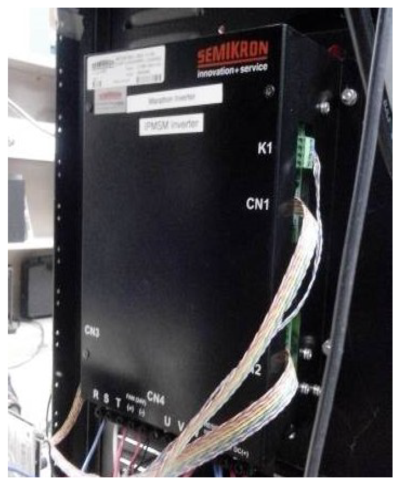
In Figure 11, the test IPMSM is controlled in a torque control mode and a load SPMSM is controlled in a speed control mode. Between the IPMSM and the SPMSM in Figure 11, a torque detector (SS-505, Ono Sokki, Yokohama, Japan) is mounted and a shaft torque of the IPMSM is measured; the torque measurement is displayed through a torque meter. During the experiment, an AIX DSP control development system (XCS2000, Analog Devices, Norwood, MA, United States) is used for controlling and sensing signals. Control algorithms are developed using C++ language and downloaded to a DSP. The line current of a motor is measured by a hall-type LEM LA 55-P current sensor and 10 kHz of PWM sampling frequency is applied during experiment. For an inverter drive, a Semikron power converter (Semitop Stack, Semikron, Nuremberg, Germany) rated for 350 Vdc and 26 A is used. Figure 12 shows the Semikron power converter used during the experiment.
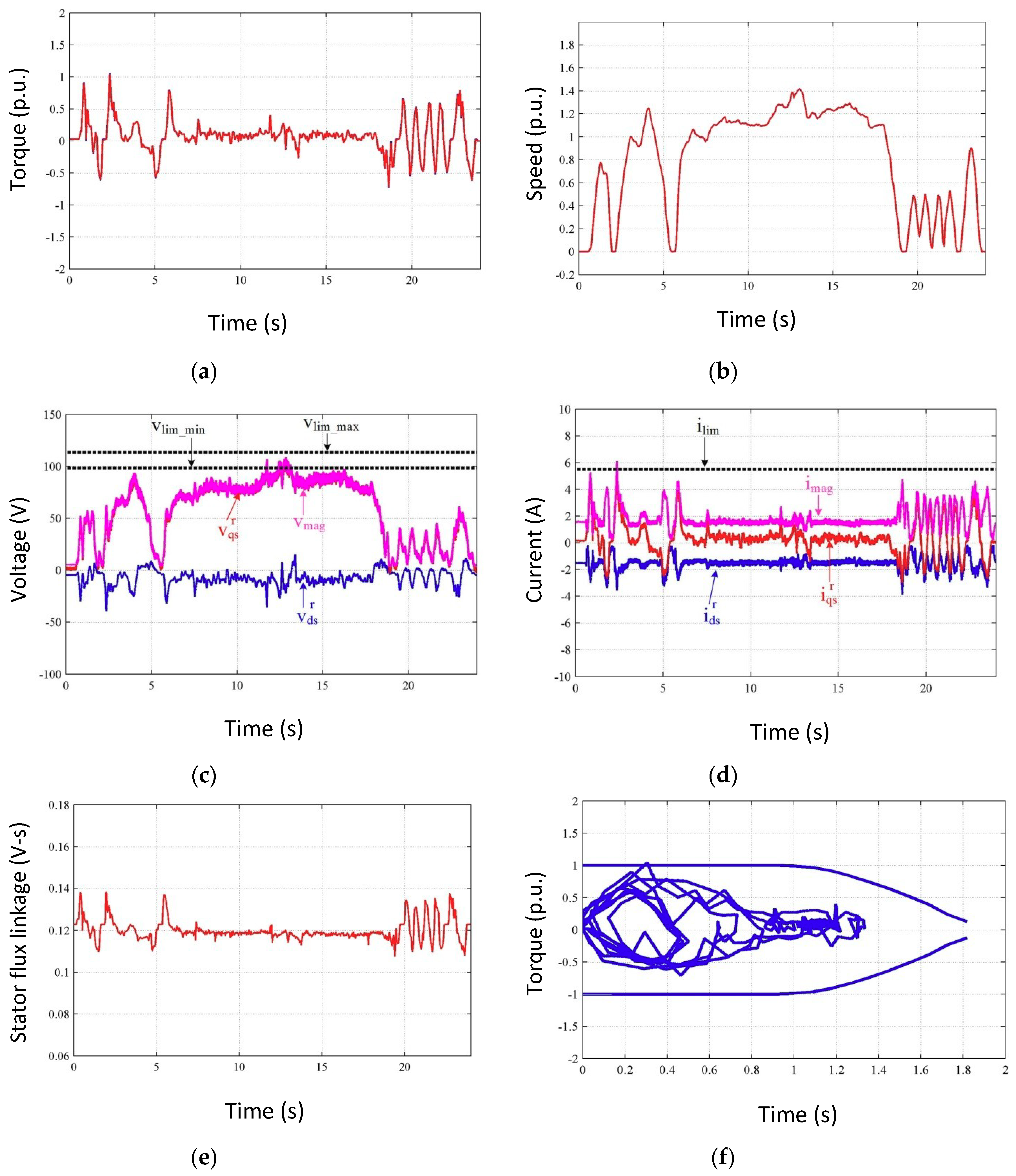
For stable operation of CVC and DB-DTFC motor drives, the US06 SFTP automotive driving cycle was applied. Rather than using actual torque and speed trajectories, the trajectories of the US06 driving cycle are scaled. During the experiment, a reduced DC link voltage is applied for safe operation of the test IPMSM drive, the load machine drive, and the torque sensor. The time range is also scaled down so that the saved data size does not exceed the memory capacity of a controller. The experimental results for the US06 SFTP automotive driving cycle using DB-DTFC are shown in Figure 13.
The torque trajectory increases up to the rated torque of the test IPMSM and the speed trajectory is increased beyond the rated speed of the test IPMSM as shown in Figure 13a,b,f. Also, the voltage and current limited operation can be observed in Figure 13c,d when the test motor drive is operated along the US06 automotive driving cycle. In Figure 13d, a rated current of the test IPMSM is marked as the current limit. A city driving cycle and a high driving cycle are combined in the US06 SFTP. Therefore, it is observed in Figure 13f that the test IPMSM operates at both low speeds and high torque conditions and at high speeds and low torque operating conditions, which correspond to a city driving cycle and a highway driving cycle, respectively.
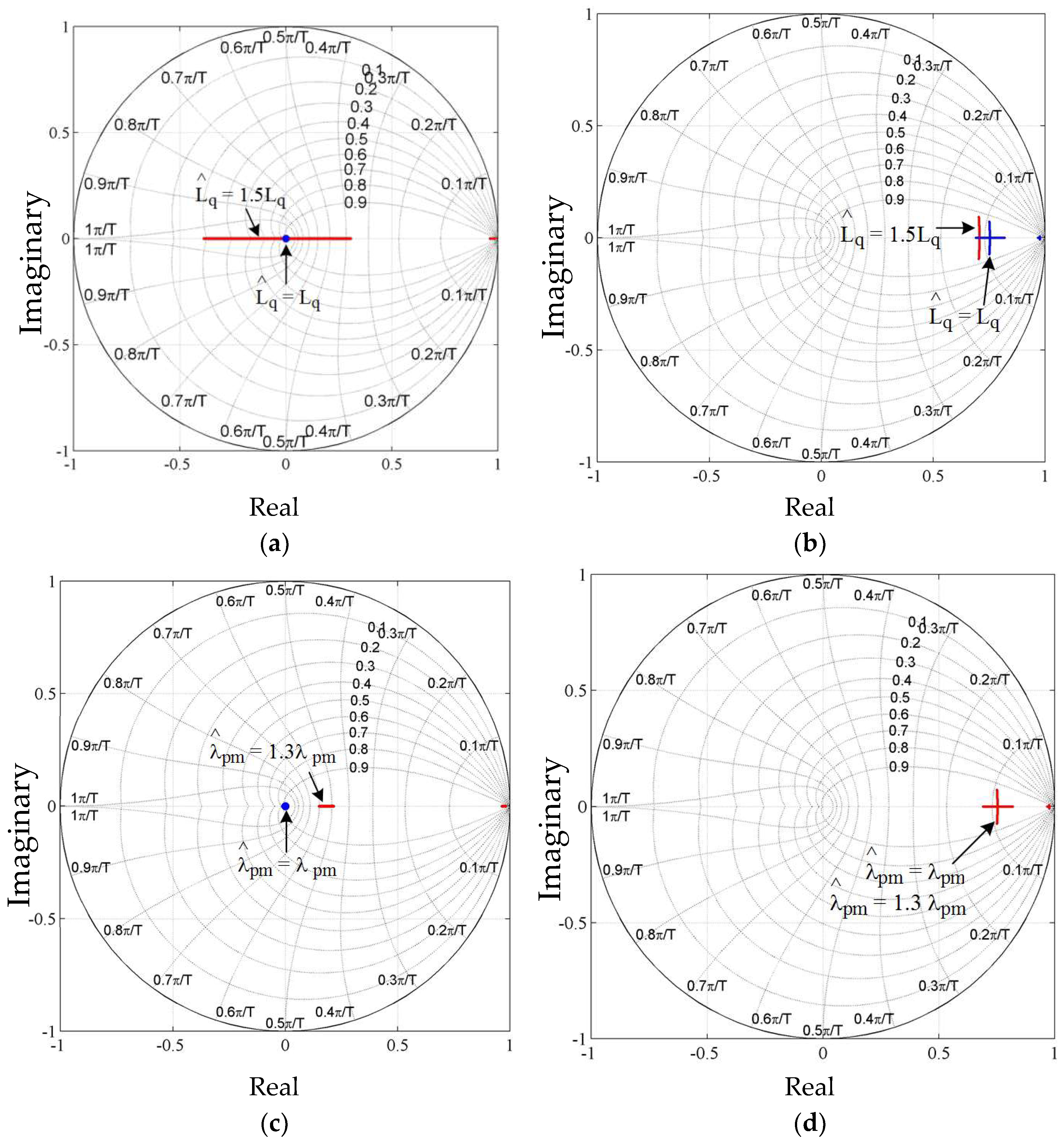
The operating point (small signal) models for the DB-DTFC and CVC IPMSM drives are derived in Equations (21) and (28), respectively. The EV migration of each motor drive is analyzed using the operating point (small signal) models derived for DB-DTFC and CVC IPMSM drives in Equations (21) and (28) and the experimental data shown in Figure 14. For evaluation of the parameter sensitivity of eigenvalue migration for each control algorithm, the q-axis inductance is detuned by 50% of its actual value and the permanent magnetic flux linkage is detuned by 30% of its actual value. The EV migration results of DB-DTFC and CVC IPMSM drives are shown in Figure 14.
Both the DB-DTFC and the CVC IPMSM drives are shown to be operating at a stable region when the torque and speed trajectories for the US06 automotive driving cycle are applied because the eigenvalues are located within the unit circle in the z-plain, as seen in Figure 14. As seen in Figure 14a,c, a deadbeat response can be achieved when the accurate estimated parameter is used. When the machine parameters, a permanent magnetic flux linkage and a q-axis inductance, are detuned, the DB-DTFC IPMSM drive still shows faster dynamic performance than the CVC IPMSM drive. However, a deadbeat response cannot be perfectly achieved, and a well-damped forced oscillation property is observed in the DB-DTFC IPMSM drive.
6. Conclusions
In this paper, the stability and dynamic characteristics of DB-DTFC and CVC IPMSM drives are analyzed with respect to machine parameter variations. Among the stability evaluation methods reviewed in Section 1, the EV migration method is applied to investigate both the stability and dynamic characteristics of each control algorithm along torque and speed trajectories of the US06 SFTP driving cycle. For eigenvalue migration of a nonlinear system, an operating point model is required. Since an IPMSM drive is a nonlinear system, the operating point models for IPMSM itself, DB-DTFC, and CVC IPMSM drive systems are derived in this paper. Using the operating point models and a driving cycle, eigenvalue migration of DB-DTFC and CVC IPMSM drives is investigated along the torque and speed trajectories of the US06 SFTP driving cycle in simulation and experiment. The simulation and experimental results show that both control systems operate within a stable region regardless of the parameter variation over the wide operating space of a motor drive system. From the simulation and experimental results of this paper, it can be concluded that the stability of a DB-DTFC IPMSM drive with respect to parameter variation is not a critical issue even though a DB-DTFC algorithm is developed for an IPMSM drive based on a machine model and parameters. When inaccurate estimated machine parameters are used for a DB-DTFC algorithm, EV migration in simulations and experiments shows that forced oscillation and well-damped responses are observed instead of a deadbeat response. However, the DB-DTFC IPMSM drive still shows faster dynamic performance than the CVC IPMSM drive, though the machine parameters, a q-axis inductance, and a permanent magnetic flux linkage are detuned within a stable operating region.
Funding
This research was funded by the Korea Electric Power Corporation [Grant number: R18XA04], the Base Science Research Program through the National Research Foundation of Korea (NRF) by the Ministry of Education (2017R1D1A1B03031979) and research funds for newly appointed professors of Chonbuk National University in 2017.
Acknowledgments
This research was supported by the Korea Electric Power Corporation [Grant number: R18XA04] and the Base Science Research Program through the National Research Foundation of Korea (NRF) by the Ministry of Education (2017R1D1A1B03031979). This research was also supported by research funds for newly appointed professors of Chonbuk National University in 2017.
Conflicts of Interest
The author declares no conflict of interest.
References
- Habetler, T.G.; Profumo, F.; Pastorelli, M.; Tolbert, L.M. Direct torque control of induction machines using space vector modulation. IEEE Trans. Ind. Appl. 1992, 28, 1045–1053. [Google Scholar] [CrossRef]
- Kenny, B.H.; Lorenz, R.D. Stator- and rotor-flux-based deadbeat direct torque control of induction machines. IEEE Trans. Ind. Appl. 2003, 39, 1093–1101. [Google Scholar] [CrossRef] [Green Version]
- Xu, W.; Lorenz, R.D. Low-sampling-frequency stator flux linkage observer for interior permanent-magnet synchronous machines. IEEE Trans. Ind. Appl. 2015, 51, 3932–3942. [Google Scholar] [CrossRef]
- Nie, Y.; Brown, I.P.; Ludois, D.C. Deadbeat-Direct Torque and Flux Control for Wound Field Synchronous Machines. IEEE Trans Ind. Electr. 2018, 65, 2069–2079. [Google Scholar] [CrossRef]
- Saur, M.; Ramos, F.; Perez, A.; Gerling, D.; Lorenz, R.D. Implementation of deadbeat-direct torque and flux control for synchronous reluctance machines to minimize loss each switching period. In Proceedings of the 2016 IEEE Applied Power Electronics Conference and Exposition (APEC), Long Beach, CA, USA, 20–24 March 2016. [Google Scholar]
- Wang, K.; Lorenz, R.D.; Baloch, N.A. Improvement of back-emf self-sensing for induction machines when using deadbeat-direct torque and flux control (db-dtfc). In Proceedings of the 2016 IEEE Energy Conversion Congress and Exposition (ECCE), Milwaukee, WI, USA, 18–22 September 2016. [Google Scholar]
- Wang, K.; Lorenz, R.D.; Baloch, N.A. Enhanced methodology for injection based real time parameter estimation to improve back-emf self-sensing in induction machine deadbeat direct torque and flux control drives. In Proceedings of the 2017 IEEE Energy Conversion Congress and Exposition (ECCE), Cincinnati, OH, USA, 1–5 October 2017. [Google Scholar]
- Pulvirenti, M.; Scarcella, G.; Scelba, G.; Lorenz, R.D. Fault tolerant capability of deadbeat—direct torque and flux control for three-phase pmsm drives. In Proceedings of the 2016 IEEE Energy Conversion Congress and Exposition (ECCE), Milwaukee, WI, USA, 18–22 September 2016. [Google Scholar]
- Kim, H.; Lorenz, R.D. Using on-line parameter estimation to improve efficiency of IPM machine drives. In Proceedings of the 2002 IEEE 33rd Annual IEEE Power Electronics Specialists Conference, Cairns, QLD, Australia, 23–27 June 2002. [Google Scholar]
- Alonge, F.; D’lppolito, F.; Feranta, G.; Ramondi, F.M. Parameter identification of induction motor model using genetic algorithms. IEE Proc. Control Theor. Appl. 1998, 145, 587–593. [Google Scholar] [CrossRef]
- Mercorelli, P. Parameters identification in a permanent magnet three-phase synchronous motor of a city-bus for an intelligent drive assistant. Int. J. Model. Identif. Control. 2014, 21, 352. [Google Scholar] [CrossRef]
- Heinbokel, B.; Lorenz, R.D. Robustness evaluation of deadbeat direct torque and flux control for induction machine driver. In Proceedings of the 2009 13th European Conference on Power Electronics and Applications, Barcelona, Spain, 8–10 September 2009. [Google Scholar]
- Lee, J.S.; Lorenz, R.D. Robustness analysis of deadbeat-direct torque and flux control for ipmsm drives. IEEE Trans. Ind. Electr. 2016, 63, 2775–2784. [Google Scholar] [CrossRef]
- Chen, L.; Mercorelli, P.; Liu, S. A Kalman estimator for detecting repetitive disturbance. In Proceedings of the 2005 American Control Conference, Portland, OR, USA, 8–10 June 2005. [Google Scholar]
- Liu, Z.; Wang, Q. Robust control of electrical machines with load uncertainty. J. Electr. Eng. 2005, 59, 760–765. [Google Scholar]
- Wai, R.J. Robust control for induction servo motor drive. IEE Proc. Electr. Power Appl. 2001, 148, 279–286. [Google Scholar] [CrossRef]
- Vaclavek, P.; Blaha, P. Lyapunov function based design of PMSM state observer for sensorless control. In Proceedings of the 2009 IEEE Symposium on Industrial Electronics & Applications, Kuala Lumpur, Malaysia, 4–6 October 2009. [Google Scholar]
- Qiang, S.; Xingming, Z.; Hongzhi, C. Limitation of the load angle for direct torque control of PMSM. In Proceedings of the 2014 IEEE Transportation Electrification Asis-Pacific (ITEC Asia-Pacific), Beijing, China, 31 August–3 September 2014. [Google Scholar]
- Luukko, J.; Pyrhonen, O.; Niemela, M.; Pyrhonen, J. Limitation of the load angle in a direct-torque-controlled synchronous machine drive. IEEE Trans. Ind. Electr. 2004, 51, 793–798. [Google Scholar] [CrossRef]
- Tsuji, M.; Kojima, K.; Mangindaan, G.M.C.; Akafuji, D.; Hamasaki, S. Stability study of a permanent magnet synchronous motor sensorless vector control system based on extended emf model. IEEJ J. Ind. Appl. 2012, 1, 148–154. [Google Scholar] [CrossRef]
- Tsuji, M.; Mizusaki, H.; Hamasaki, S. Stability comparison of ipmsm sensorless vector control systems using extended emf. In Proceedings of the 2014 International Power Electronics Conference (IPEC-Hiroshima 2014-ECCE ASIA), Hiroshima, Japan, 18–21 May 2014. [Google Scholar] [CrossRef]
- Guha, A.; Narayanan, G. Small-signal stability analysis of an open-loop induction motor drive including the effect of inverter deadtime. IEEE Trans. Ind. Appl. 2016, 52, 242–253. [Google Scholar] [CrossRef]
- Grdenić, G.; Delimar, M. Small-Signal Stability Analysis of Interaction Modes in VSC MTDC Systems with Voltage Margin Control. Energies 2017, 10, 873. [Google Scholar] [CrossRef]
- Zhang, B.; Yan, X.; Li, D.; Zhang, X.; Han, J.; Xiao, X. Stable Operation and Small-Signal Analysis of Multiple Parallel DG Inverters Based on a Virtual Synchronous Generator Scheme. Energies 2018, 11, 203. [Google Scholar] [CrossRef]
- Park, C.; Lee, J. A torque error compensation algorithm for surface mounted permanent magnet synchronous machines with respect to magnet temperature variations. Energies 2017, 10, 1365. [Google Scholar] [CrossRef]
- Slotine, J.; Li, W. Applied Nonlinear Control; Prentice Hall: Upper Saddle River, NJ, USA, 1991; p. 199. [Google Scholar]
- Lee, J.S.; Lorenz, R.D. Deadbeat-direct torque and flux control of ipmsm drives using a minimum time ramp trajectory method at voltage and current limits. In Proceedings of the 2013 IEEE Energy Conversion Congress and Exposition, Denver, CO, USA, 15–19 September 2013. [Google Scholar] [CrossRef]
Figure 1.
Stationary and rotor reference frame notation of a PMSM (permanent magnet synchronous motor).
Figure 1.
Stationary and rotor reference frame notation of a PMSM (permanent magnet synchronous motor).
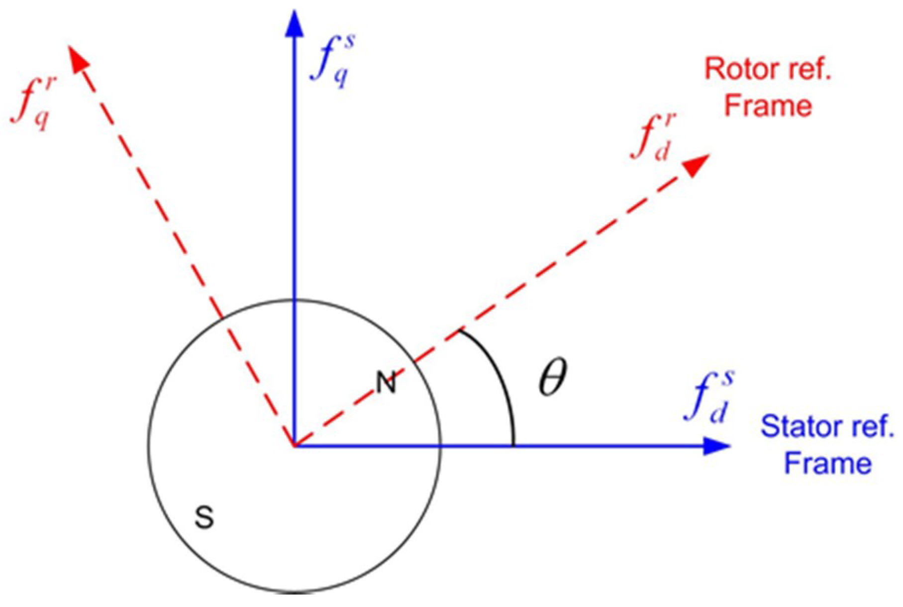
Figure 2.
A block diagram of a stator current observer in a discrete time domain.

Figure 3.
Estimation accuracy characteristic of a stator current observer with respect to q-axis inductance variation at a frequency domain [3]. (a) Magnitude of estimation accuracy; (b) Phase of estimation accuracy.
Figure 3.
Estimation accuracy characteristic of a stator current observer with respect to q-axis inductance variation at a frequency domain [3]. (a) Magnitude of estimation accuracy; (b) Phase of estimation accuracy.
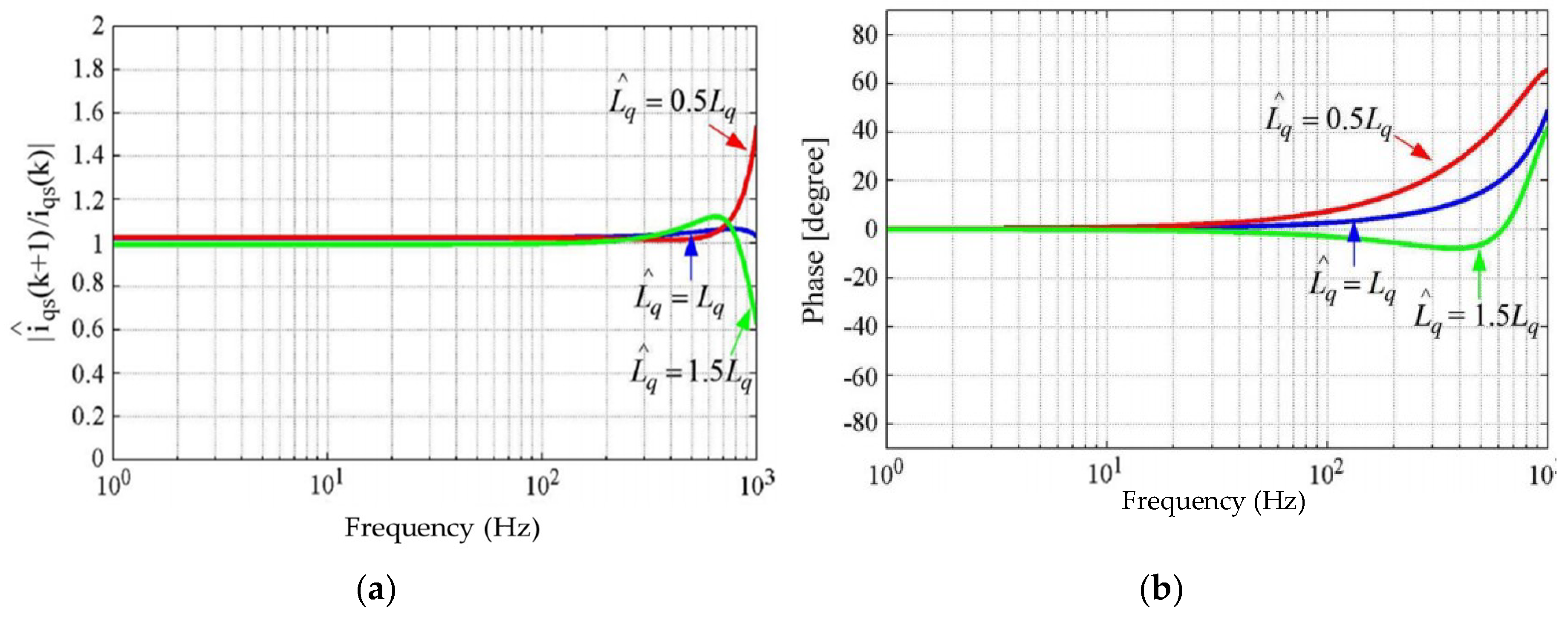
Figure 4.
A block diagram of a stator flux linkage observer used for DB-DTFC (deadbeat-direct torque and flux control) implementation [25].
Figure 4.
A block diagram of a stator flux linkage observer used for DB-DTFC (deadbeat-direct torque and flux control) implementation [25].
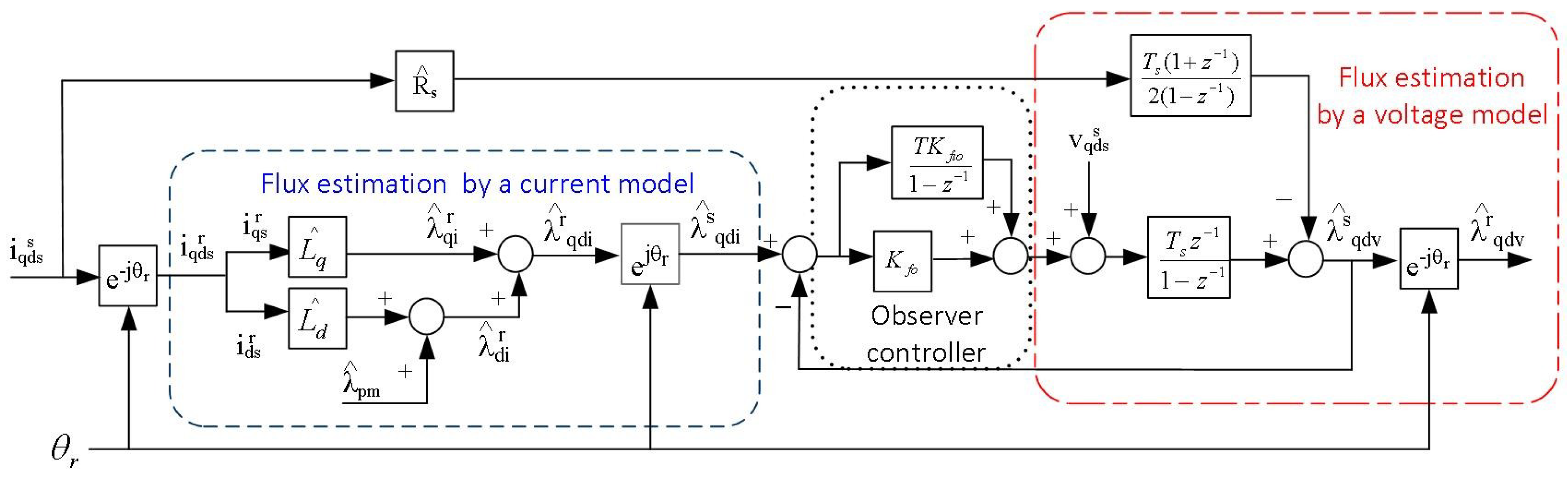
Figure 5.
Simulation results of a frequency response of the stator flux linkage observer with respect to motor parameter variations [25].
Figure 5.
Simulation results of a frequency response of the stator flux linkage observer with respect to motor parameter variations [25].

Figure 6.
A block diagram of a DB-DTFC IPMSM (interior permanent magnet synchronous motor) drive.
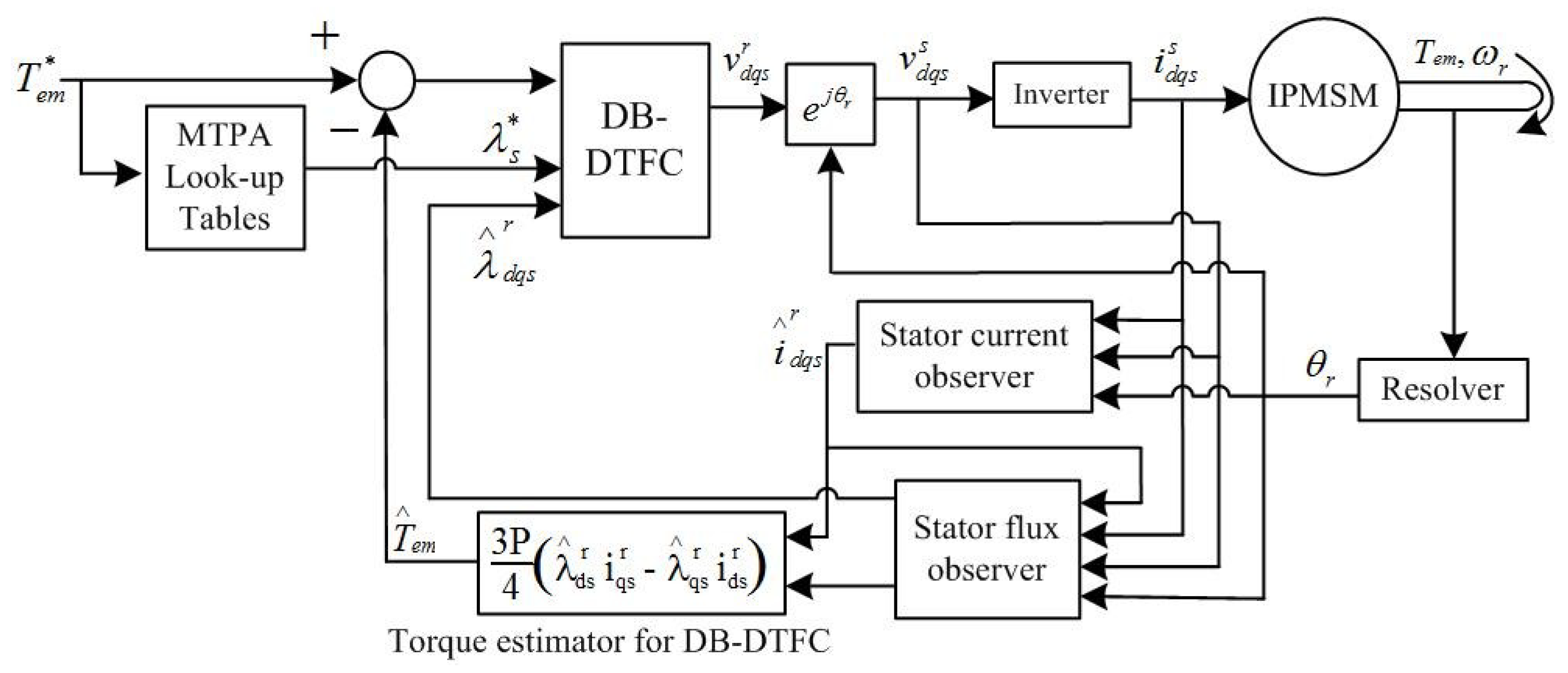
Figure 7.
A block diagram of an MTPA (maximum torque per ampere) based CVC IPMSM drive.

Figure 8.
Simulation results of motor dynamics along the US06 SFTP (supplemental federal test procedure) driving cycle. (a) Torque; (b) Speed; (c) Voltage; (d) Current; (e) Stator flux linkage; (f) Torque-speed.
Figure 8.
Simulation results of motor dynamics along the US06 SFTP (supplemental federal test procedure) driving cycle. (a) Torque; (b) Speed; (c) Voltage; (d) Current; (e) Stator flux linkage; (f) Torque-speed.
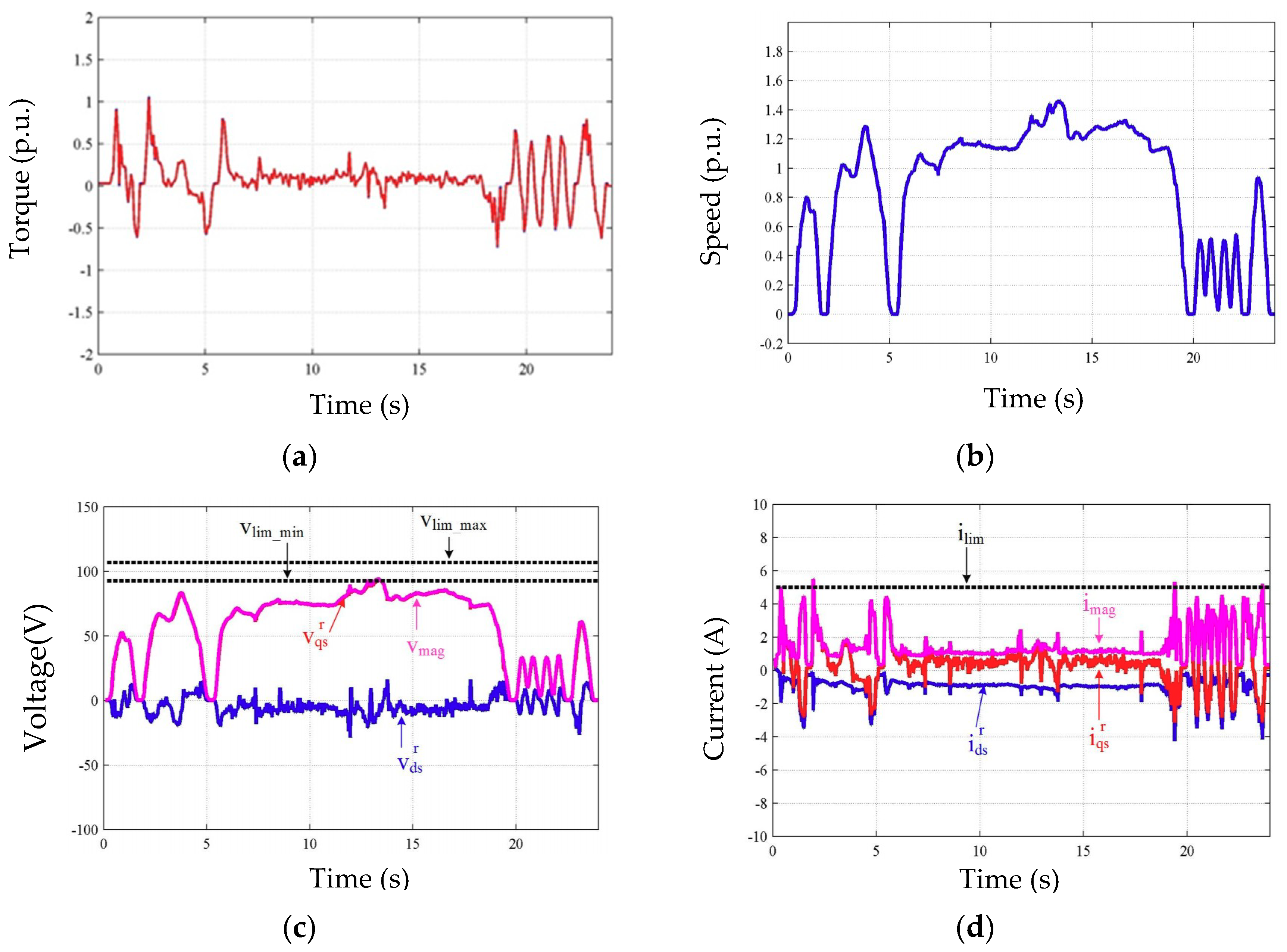

Figure 9.
Eigenvalue (EV) migration of DB-DTFC and CVC along the U.S.06 driving cycle when and are detuned by 50% and 30%, respectively. (a) When Lq is detuned in DB-DTFC; (b) When Lq is detuned in CVC; (c) When λpm is detuned in DB-DTFC; (d) When λpm is detuned in CVC.
Figure 9.
Eigenvalue (EV) migration of DB-DTFC and CVC along the U.S.06 driving cycle when and are detuned by 50% and 30%, respectively. (a) When Lq is detuned in DB-DTFC; (b) When Lq is detuned in CVC; (c) When λpm is detuned in DB-DTFC; (d) When λpm is detuned in CVC.

Figure 10.
Corresponding impulse responses with respect to EV locations specified in Figure 9a,b. (i) deadbeat response; (ii) forced oscillation; (iii) underdamped response of DB-DTFC; (iv) underdamped response of CVC.
Figure 10.
Corresponding impulse responses with respect to EV locations specified in Figure 9a,b. (i) deadbeat response; (ii) forced oscillation; (iii) underdamped response of DB-DTFC; (iv) underdamped response of CVC.

Figure 11.
Experimental test set-up.

Figure 12.
A Semikron power converter.

Figure 13.
Experimental results of dynamics of the DB-DTFC IPMSM drive along the US06 SFTP driving cycle. Operating conditions: = 10 (kHz) and = 170 (V). (a) Torque; (b) Speed; (c) Voltage; (d) Current; (e) Stator flux linkage; (f) Torque-speed.
Figure 13.
Experimental results of dynamics of the DB-DTFC IPMSM drive along the US06 SFTP driving cycle. Operating conditions: = 10 (kHz) and = 170 (V). (a) Torque; (b) Speed; (c) Voltage; (d) Current; (e) Stator flux linkage; (f) Torque-speed.

Figure 14.
Eigenvalue (EV) migration of DB-DTFC and CVC along the US06 driving cycle when and are detuned by 50% and 30%, respectively. (a) When Lq is detuned in DB-DTFC; (b) When Lq is detuned in CVC; (c) When λpm is detuned in DB-DTFC; (d) When λpm is detuned in CVC.
Figure 14.
Eigenvalue (EV) migration of DB-DTFC and CVC along the US06 driving cycle when and are detuned by 50% and 30%, respectively. (a) When Lq is detuned in DB-DTFC; (b) When Lq is detuned in CVC; (c) When λpm is detuned in DB-DTFC; (d) When λpm is detuned in CVC.

Table 1.
Comparison of CVC (current vector control) and DB-DTFC (deadbeat-direct torque and flux control) based on results in Figure 8.
Table 1.
Comparison of CVC (current vector control) and DB-DTFC (deadbeat-direct torque and flux control) based on results in Figure 8.
| Characteristic | CVC | DB-DTFC |
|---|---|---|
| Complexity | Medium | High |
| Computation time using a diginal signal processor (DSP) [27] | 31.4 (μs) | 34 (μs) |
| Command tracking | Satisfactory | Satisfactory |
| Efficient operation | Satisfactory | Satisfactory |
Table 2.
IPMSM (interior permanent magnet synchronous motor) specifications.
| Parameter | Value | Parameter | Value |
|---|---|---|---|
| 1.4 (Ω) | Rated Power | 1.5 (kW) | |
| 0.121 (Volt-s) | Rate Torque | 2.26 (N.m.) | |
| 8.5 (mH) | Rated Speed | 6200 (rpm) | |
| 20 (mH) | Rated current (Continuous) | 5.5 (A) | |
| Poles | 4 | Max. current (Instantaneous) | 17 (A) |
| 100 (μs) | 1.0 (kg⋅m2 × 10−4) |
© 2018 by the author. Licensee MDPI, Basel, Switzerland. This article is an open access article distributed under the terms and conditions of the Creative Commons Attribution (CC BY) license (http://creativecommons.org/licenses/by/4.0/).
Share and Cite
MDPI and ACS Style
Lee, J.S. Stability Analysis of Deadbeat-Direct Torque and Flux Control for Permanent Magnet Synchronous Motor Drives with Respect to Parameter Variations. Energies 2018, 11, 2027. https://doi.org/10.3390/en11082027
AMA Style
Lee JS. Stability Analysis of Deadbeat-Direct Torque and Flux Control for Permanent Magnet Synchronous Motor Drives with Respect to Parameter Variations. Energies. 2018; 11(8):2027. https://doi.org/10.3390/en11082027
Chicago/Turabian StyleLee, Jae Suk. 2018. "Stability Analysis of Deadbeat-Direct Torque and Flux Control for Permanent Magnet Synchronous Motor Drives with Respect to Parameter Variations" Energies 11, no. 8: 2027. https://doi.org/10.3390/en11082027
Note that from the first issue of 2016, this journal uses article numbers instead of page numbers. See further details here.