Assessing the Demand Side Management Potential and the Energy Flexibility of Heat Pumps in Buildings


1
Università eCampus, via Isimbardi 10, 22060 Novedrate (CO), Italy
2
Dipartimento di Ingegneria Industriale e Scienze Matematiche, Università Politecnica delle Marche, via brecce bianche 1, 60131 Ancona, Italy
*
Author to whom correspondence should be addressed.
Energies 2018, 11(7), 1846; https://doi.org/10.3390/en11071846
Submission received: 29 June 2018
/
Revised: 8 July 2018
/
Accepted: 13 July 2018
/
Published: 14 July 2018
(This article belongs to the Special Issue Refrigeration, Air Conditioning and Heat Pumps: Energy and Environmental Issues)
Abstract
:The energy demand in buildings represents a considerable share of the overall energy use. Given the significance and acknowledged flexibility of thermostatically controlled loads, they represent an interesting option for the implementation of demand side management (DSM) strategies. In this paper, an overview of the possible DSM applications in the field of air conditioning and heat pumps is provided. In particular, the focus is on the heat pump sector. Three case studies are analyzed in order to assess the energy flexibility provided by DSM technologies classified as energy efficient devices, energy storage systems, and demand response programs. The load shifting potential, in terms of power and time, is evaluated by varying the system configuration. Main findings show that energy efficient devices perform strategic conservation and peak shaving strategies, energy storage systems perform load shifting, while demand response programs perform peak shaving and valley filling strategies.
1. Introduction
Energy consumption in the residential sector represents about 40% of the total energy use both in Europe and in the US [1,2]. In particular, heating and cooling in buildings have a high share of the overall energy use. Air conditioners are responsible on average for around 5% of global electricity consumption, with a variable percentage country by country (e.g., 14% in the US and 40% in India) [3], and such share is expected to grow due to the increasing refrigeration demand also due to global warming. The relevance of heat pumps is also increasing; in 2015 about 800,000 units were sold in Europe and a growing trend in sales is estimated for the coming years [4]. Nevertheless, buildings are considered a resource in power systems thanks to the high energy flexibility they promise. Indeed, in buildings there are several deferrable loads (e.g., laundry machines and dish washers) and thermostatically controlled loads (TCL), such as heat pumps, refrigerators, and air conditioners. The latter technologies, especially, contain various forms of storage, which can be used to alter the electric load without affecting the quality of the energy service [5]. The energy flexibility provided by buildings is paramount to mitigate the upcoming challenges of future power systems, and its exact definition and quantification has a central role, as stated by the working group of Annex 67 about energy flexible buildings [6]. Furthermore, the EU’s Energy Performance of Buildings Directive [7] pushes towards new and more performing buildings—nearly zero energy buildings (nZEB)—where energy efficiency and energy flexibility are essential to achieve the required performance targets.
Given this premise, the sector of heating and cooling in buildings is promising for the application of demand side management (DSM) strategies aimed at modifying the final user’s electricity demand on the basis of electricity grid needs. The relevance of DSM is related to the growing share of renewable energy sources (RES) in the generation mix and consequently to the necessity of integrating them and of adapting the energy demand to their intermittent and unpredictable production. Besides this aspect, DSM can produce several other advantages in the electric power system, which can be summarized as [8]: reduced need for increasing the power generation capacity; higher operational efficiency in production, transmission, and distribution of electric power; and lower electricity costs. A DSM strategy can have different purposes, such as peak shaving, valley filling, load shifting, energy conservation, and strategic load growth [9].
DSM technologies can be used to activate the energy flexibility of buildings. They can be divided into three main categories: (i) energy-efficient end-use devices; (ii) additional equipment, systems, and controls to enable load shaping (e.g., energy storage); and (iii) communication systems between end-users and external parties, for example, demand response (DR) programs [9]. While the first point concerns energy conservation by means of devices using less energy, the other two points deal with systems aimed at shifting the final user’s demand: thermal energy storage systems can be used to store surplus energy to be released for later use, whereas demand response achieves changes in final users’ load by means of price signals from the grid.
The purpose of this paper is to highlight how DSM technologies for air conditioning and heat pumps can unlock the energy flexibility in buildings and to show, consequently, which kind of DSM strategy can be fulfilled through them. A state of the art review is presented to illustrate the existing trend in the implementation of the above mentioned DSM categories (Section 2), that is, (i) energy efficiency, (ii) energy storage systems, and (iii) demand response programs. In this way, a holistic overview of the potential for managing the energy demand related to cooling or heating loads is provided. Considering the relevance in terms of share on global energy use and units sold worldwide, and the increasing importance of electric energy among the final uses, a particular focus is on the heat pump sector. Three different case studies for each of the considered DSM categories are analyzed and the consequent energy flexibility is quantified by means of flexibility indicators available in the literature and illustrated in Section 3. Indeed, it is shown that several indicators for energy flexibility quantification have been introduced; here the main novelty lays in the application of the most meaningful to compare the flexibility potential of different DSM technologies. By means of these case studies, an in-depth analysis on more efficient devices, energy storage systems, and DR actions is performed and their effect in terms of modification of energy demand load shape is discussed (Section 4). Some conclusions about unlocking energy flexibility are drawn on the basis of the obtained results (Section 5).
2. State of the Art Review of DSM Technologies for Air Conditioning and Heat Pumps
In this section, the process of how demand side management can be realized in the HVAC (heating ventilation and air conditioning) sector is discussed. Chillers and heat pumps, as said, belong in the category of thermostatically controlled loads: they are aimed at keeping the operative temperature in a given range and they allow the shift of thermal loads produced by electricity conversion, thanks to inherent or external thermal energy storages. The results of the literature review are divided on the basis of the above-mentioned categorization of DSM technologies: energy efficiency, energy storage, and demand response. Main findings are summarized in Table 1 and are discussed in detail in the following sections.
2.1. Energy Efficiency
Energy efficiency in reverse cycle devices (i.e., heat pumps and chillers) can be achieved in several ways. It is possible to act on: (i) the choice of a proper and environmental friendly refrigerant; (ii) more efficient design of components (variable speed compressors, variable refrigerant flow, ejectors); (iii) application of not-in-kind technologies; and (iv) optimization of the overall HVAC system and control strategies.
In the literature there are several studies that deal with the above mentioned topics. In the following, some of them are reported:
- The use of natural refrigerants is gaining more and more interest. Harby [10] focuses, for example, on the problems (environmental impacts and energy use) associated with the use of halogenated refrigerants and the possibility to replace them with hydrocarbons (HC). The author provides a guide to understand the current status, replacement strategy of conventional refrigerants, and possible drawbacks in using HC. Bolaji and Huan [11] review existing natural refrigerants (HC, ammonia, CO2, water) and their areas of application in refrigeration and air-conditioning systems. They show the potential of natural refrigerants to replace halogenated refrigerants. Nawaz et al. [12] propose propane and isobutene as natural refrigerants for heat pump water heaters, while Zajacs et al. [13] analyze the possibility of using ammonia in a heat pump for space heating and domestic hot water production.
- Among the other technologies, variable capacity compressors are considered as an effective way to achieve energy efficiency for air-conditioning chillers and heat pumps. Krishnamoorthy et al. [14] present the cooling operation of a variable-capacity/variable-fan-speed heat pump and they show its potential to reduce residential energy use, highlighting also the importance of location and insulation level of the duct system. Park et al. [15] evaluate the performance of a variable refrigerant flow (VRF) air conditioning (AC), that is, an air-conditioning system able to control the amount of refrigerant flowing to the multiple evaporators (indoor units). They assess energy use and comfort of occupants for a Korean building and obtained results confirming the advantages of a VRF system. Aynur et al. [16] compare a VRF AC system with a variable air volume (VAV) AC and assess a potential energy saving between 27% and 58% depending on the system configuration, and indoor and outdoor conditions. Özahi et al. [17] show for a real case that variable refrigerant flow systems can produce a 44% cost saving compared to traditional HVAC systems. Among the ways of improving the performance of a vapor compression refrigeration cycle, using an ejector as an expansion device is one of the possibilities [18]. The ejector is a machine without movable organs that can be used as a compressor and as a pump to achieve a pressure rise of a given fluid through supply of another fluid with the same or different nature. Wang et al. [19] describe a hybrid ejector air-conditioning system and its optimization. The proposed system has the compressor installed between the outlet of evaporator and ejector secondary flow inlet. The optimization of such a system leads to a 7% energy use reduction. Boccardi et al. [20], instead, evaluate the performance improvement due to an ejector in a HVAC system working with CO2 as refrigerant. The optimal configuration of the system is determined.
- Not-in-kind technologies category includes the following technologies for domestic applications: thermoacoustic refrigeration, thermoelectric refrigeration, thermotunneling, magnetic refrigeration, Stirling cycle refrigeration, pulse tube refrigeration, Malone cycle refrigeration, absorption refrigeration, adsorption refrigeration, and compressor driven metal hydride heat pumps [21]. Among all the others, magnetic refrigeration shows fast developments in new materials and system architecture, and it is considered very promising as an alternative to some conventional cooling, refrigeration, and air-conditioning technologies [22].
- Energy recovery is of paramount importance to increase the efficiency of an HVAC and it can be performed, for example, by means of an enthalpy wheel or heat exchangers, whose performance can be enhanced by the inclusion of phase change material (PCM) [23]. Du et al. [24], instead, analyze different control strategies for achieving energy savings with a HVAC system in an airport. They make a comparison on the basis of an exergy based method. Ascione et al. [25] present a methodology for the optimization of a building-HVAC system by employing a model predictive control (MPC) strategy for heating and cooling. The authors show a primary energy saving around 35.4 kWh/m2 for a residential building in Southern Italy. Indeed, several studies have shown that by adding a supervisory MPC controller to HVAC systems could result in energy use and operating cost reductions from 7% to more than 50% [26,27,28].
2.2. Energy Storage
The relevance of coupling reverse cycle devices with thermal energy storage in order to modify the final user’s demand and match it with the power system production has been demonstrated in the literature [29].
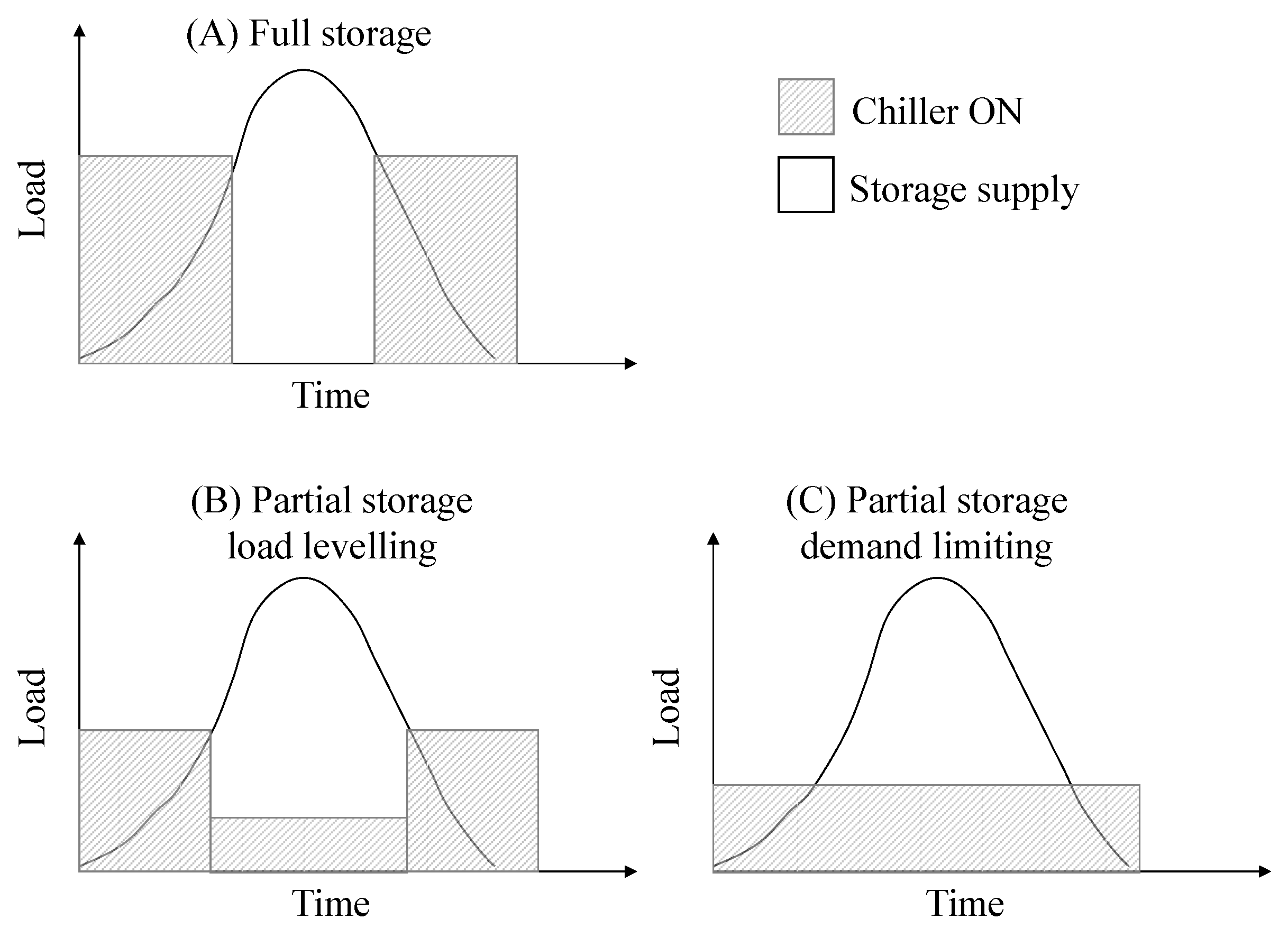
A cold thermal energy storage (CTES) can be coupled to a chiller for air conditioning. It can be a thermally stratified chilled water storage (sensible TES) or an ice storage (latent TES) [30]. A TES can convey several benefits: improving the refrigeration equipment efficiency, reducing the installed capacity, increasing the operational flexibility, and reducing energy costs, because cold is produced during off-peak periods and used during on-peak periods. Typical operational strategies of such systems are full storage and partial storage strategies, as shown in Figure 1 [31].
Partial storage is the most used configuration because of lower initial capital costs. It saves about 40–60% of peak cooling electricity demand. Full storage is interesting for short peak periods with very high costs for electricity production. The peak electricity demand can be reduced by up to 80–90% [32]. Similarly, thermal energy storage systems can be coupled with heat pumps for implementing demand side management strategies [33], such as peak shaving or night load shifting. These kinds of applications can lead to energy bill reductions, even if generally the energy use increases because of thermal losses in the storage systems.
Rather than the use of external storage tanks, also much more effective in buildings, there is the use of the building envelope—thermal mass as passive or active energy storage [34]. Floor heating or TABs (thermally activated buildings) are active thermal storage systems [35]: the floor is a large, low temperature radiating surface while the concrete acts like a thermal storage heated by air, water, or directly by electric resistances. The building envelope, instead, is passive thermal storage, easily exploited by means of variable inside temperature set-points, which can be adjusted in a certain range in order to maintain the internal comfort and, at the same time, provide useful flexibility to the power system [36]. Furthermore, PCM can be integrated within the building components and used passively, for pre-cooling or pre-heating and for reducing the thermal load request, or alternatively used actively, by charging and discharging their energy content on the basis of a given strategy.
2.3. Demand Response
Among the other devices, reversible heat pumps (for heating and cooling) are recognized as systems to be effectively used to implement demand response strategies in the smart grid. Demand response strategies are mainly aimed at three different purposes: (i) provision of ancillary services for the power grid, (ii) renewable energy sources integration, and (iii) energy bill reduction for the final user [37].
- Ancillary services consist of frequency and voltage control, congestion management, and provision of spinning and non-spinning reserve [37]. In voltage control applications, heat pump load is modified to maintain the distribution network voltage within the allowed limits: heat pump (HP) active power demand is decreased in times of local under-voltage and increased in times of over-voltage. The latter case can happen, for example, in presence of photovoltaic (PV) panels, feeding electricity in the grid. In a similar manner, frequency control can be realized to ensure that the grid frequency stays within a specific range of the nominal frequency. An existing example of application is the virtual energy storage network, named “tiko”, which connects more than 10,000 electric heating devices (i.e., heat pumps and water heaters) throughout Switzerland [38]. As far as congestion management in the distribution grid is concerned, optimized scheduling and power rating of heat pumps are paramount in order to avoid limitations in the transformer and line capacity [37,39]. Eventually heat pumps can serve as spinning and non-spinning reserves used by the transmission system operator (TSO) [37,40], that is, as reserve capacity that can be regulated downward or upward to match demand and supply. Different strategies can be implemented with these reserves, such as peak clipping or valley filling. In References [41,42,43], incentive based DR programs are considered to provide ancillary services to the power system by means of active demand and their influence on the real power markets is assessed.
- Another important role played by heat pumps and the flexibility they provide is related to the possibility to integrate renewable energy sources both at building level and at power system level. The main RES considered are wind and PV. Bruninx [40] shows the impact on wind utilization factor (WUF) produced by heat pumps adhering to a DR program: on average, the WUF increases from about 75% in the reference case to 84% when heat pumps are used as operational reserves. This increase of WUF is the result of shifting demand to periods of excess wind power generation and of increasing the indoor temperature in order to allow the DR adherent heating systems to provide upward reserves. Baetens et al. [44] demonstrate the positive role of heat pumps to reduce curtailment of electricity from PV panels. Arteconi et al. [45] show how heat pumps coupled with thermal storage can increase the self-consumption of PV electricity production in an industrial building. In this study, the tank operative conditions are analyzed in order to find the best configuration: up to 80% of PV electricity can be used to cover the thermal demand coming from the building.
- Regarding energy bill reduction, electricity price signals are used to influence the final user’s consumption pattern. Mainly, there are two types of tariff structures: Time of Use (TOU) tariffs, varying on the period of the day, and Real Time Pricing (RTP), changing with the electricity market price [46]. The heat pump demand can be shifted driven by the price with the intent of reducing electricity costs, improving the system performance, increasing RES integration, or improving power system benefits (i.e., reducing total operational costs). It is evident how the final users and power system interests are strictly related. However, it has been demonstrated that the benefit that a final user can achieve in taking part in a DR program depends also on the number of participants: the operational cost reduction per participant drops when increasing the penetration of DR programs because less flexibility is requested of each user. In more detail, the total cost savings have been assessed at most between about 400 € to 200 € per participant per year for a 5% and 100% DR penetration rate, respectively [47]. In Reference [48], price-controlled energy management of smart homes (SHs) is investigated and it is demonstrated that the benefit for both the generation scheduling problem and for the final users, is a decrease in operational costs. Even in Reference [49], demand response programs are modeled in the unit commitment (UC) problem in order to evaluate achievable operational costs savings.
3. Methods
In the following, three particular DSM technologies, among those above mentioned, were studied. They were chosen on the basis of their widespread and technological relevance. Variable capacity heat pumps were considered as energy efficient devices; thermally stratified water tanks as storage systems; and real time pricing as demand response programs. Firstly, the flexibility assessment procedures available in the literature are listed and the load shifting indicator used here is described in detail. Secondly, the three case studies selected are presented. Eventually, the behavior of the three systems in the presence of the DSM technology is analyzed, and results for the different cases are discussed and compared.
3.1. Flexibility Evaluation
The flexibility provided by heating and cooling systems in buildings is intended as the power consumption deviation of the heating or cooling device from its optimal value (or normal operation) to a new profile aimed at compensating power imbalances in the grid. Such new load patterns can be obtained by using heat buffers where heat or cold can be stored when a surplus of electricity is available and vice-versa. In this context, heat buffers are mainly represented by thermal energy storage and building thermal mass.
There are several studies in the literature that have proposed ways to quantify this flexibility as:
- number of hours the energy use can be delayed or anticipated [50];
- power increase or decrease and time duration of its variation within functional and comfort limits [51];
- energy cost, based on cost functions, which represent how much shifting the energy use costs [52];
- ratio between the maximum change in power to the additional energy use in a certain period (efficiency curves) [53];
- power demand versus priority to be supplied in order to satisfy the operational constraints (priority curves) [54];
- maximum heat that can be stored in the structural storage capacity of a building without violating the thermal comfort [55];
- hourly (h) load shed potential of a device with respect to its rated power consumption (Pbase) during a DR event (DRp), as shown in Equation (1) [36]:
It is evident that different energy flexibility indicators have been proposed and a unique definition does not exist [6]. The most used variables to characterize the flexibility are the amount of power change, duration of the change, rate of change, response time, shifted load and maximal hours of load shifted, and recovery time (which represents when the system is ready to be used again) [56]. The energy flexibility can be evaluated at the design stage, as an intrinsic value related to the building and its heating and cooling system features, or during its operational behavior. The first evaluation is important to have an overall idea of the maximum potential flexibility related to building energy systems, while the second one is useful to assess what happens during operation, especially in case of a specific event, such as a DR control signal sent to the building. In the latter case, the most relevant parameters to take into account during the evaluation are temporal flexibility, power capacity, and energy shifted [57].
In this study, not the normal operation of a system, but the effect of the substitution of a conventional system with another with a higher flexibility potential (i.e., a DSM technology) is considered. The operational behavior is analyzed to evaluate the impact of the DSM technology on the DSM strategy that can be implemented through it. The energy flexibility indicator chosen strictly depends on the purpose of its use. Among others, the number of hours the energy use can be shifted and the hourly load shed potential are indicators highly appropriate to assess the effects of a specific DSM technology. Indeed, from the electricity grid perspective, how the power demand can be modified and for how much time are the most important pieces of information. In the following sections, some case studies where DSM technologies are introduced, are analyzed. The flexibility indicators used are the time shifting and the load shifting potential. The time shifting (tS) can be assessed by comparing the energy cumulative curves in the case with and without DSM implementation (i.e., the horizontal distance between the curves). Whereas the load shifting potential for the DSM technology, useful when the dynamic operation is evaluated, is calculated similarly to DRp [36] as follows:
where LSDSM,t is the load shifting potential for the considered DSM technology at the time step t, PtDSM is the power consumption at the time step t when the DSM technology is in place, while PtnoDSM is the power consumption at the time step t without any DSM technology. LSDSM,t is positive when the introduction of the DSM technology increases the power load at the considered time step (when PtnoDSM is zero, then LSDSM,t is 100%); it is negative when the DSM technology reduces the power consumption.
3.2. Case Studies
Three different case studies were considered to evaluate the energy flexibility available when a DSM technology was implemented in comparison with reference cases without DSM. In particular, given the relevance of the energy use in the building sector [7] and the increasing market penetration of heat pumps as heating and cooling devices [4], the presented case studies analyzed the implementation of different configurations of heat pump systems in residential buildings. Indeed, it is highly recognized also in Italy the potential of heat pumps as electric heating systems to perform primary energy savings [58]. The energy flexibility is provided by:
- a HP energy efficient design (variable capacity HP),
- a thermally stratified water tank,
- a DR program based on dynamic pricing
and is quantified by means of the above mentioned flexibility indicators. Different types of buildings, heating and cooling systems, and distribution systems were considered in order to make broader the evaluation of the energy flexibility associated with heat pump operation. In particular, the building specifications and generation and distribution characteristics have been chosen to be congruent among them, and with the DSM technology implemented. The buildings were assumed located in a town of central Italy (Ancona). The purpose of the analysis being a qualitative evaluation of the kind of flexibility provided by different DSM technologies, results are shown for a representative winter’s day. The inside temperature set-point was set at 20 °C (±0.5 °C) to be maintained 24 h per day. It was assumed about 30 m2 per person, which provided an internal gain of 120 W each. A 0.5 ACH (air changes per hour) was modelled. The heat pump performance was obtained from manufacturer’s data [59], where the heat pump compressor power consumption was given by varying the evaporator and condenser temperature in relation to the indoor and ambient temperatures. TRNSYS [60] was the tool used for the dynamic simulations. It is widely used for building simulation and it has been thoroughly tested, thus its results can be considered reliable in respect to the issue of model validation, which has a paramount relevance as highlighted in Reference [61]. The simulations time step was 6 min. The case studies are discussed in detail in the following sections. In Table 2 the building properties for each case study are reported; buildings have been represented with a regular shape (parallelepiped). In Table 3 the design parameters of the heating systems are summarized.
3.2.1. Case A: Energy Efficiency
Case A assessed the flexibility due to an efficient design of the heat pump, that is, a variable capacity heat pump was used. A multi-apartment residential building with a ground coupled heat pump (GCHP) as a heating production system was considered (Figure 2a). It had been modelled in TRNSYS by means of Type 56 for buildings with active layers, while Type 927 for water-to-water heat pumps has been used, acting on the scale factor to simulate the variable capacity, which was coupled to Type 557 for the borefield. Given the novelty of this kind of building in Italy, a new building highly insulated [63] was assumed (see Table 2), having a total floor area of 1000 m2. Underfloor space heating was used. A 1000 L thermal energy storage was installed to decouple energy production and consumption and to guarantee that space heating was supplied with warm water within a given temperature range (20–40 °C). The heat pump design heating capacity has been assessed at 8 kW, as 70% of the design thermal power (evaluated at the design outside temperature of −1 °C and inside temperature of 20 °C). Indeed, it is common practice in heat pump generation systems with underfloor heating systems to size the heating capacity a bit lower than the design value, given the low occurrence of the design outdoor temperature. In this way, the heat pump is not too oversized for the average operating conditions and a back-up generator can be included for peak power demand. In this exercise, the flexibility provided by the energy efficient design of the heat pump was evaluated: the performance of a variable capacity heat pump, which can reduce its load up to 30% of the design value, was compared to an ON-OFF heat pump. The control logic switches on the heat pump when the ambient temperature is lower than 15 °C and the tank temperature goes lower than the upper bound. In presence of the variable capacity heat pump, the capacity was assessed on the basis of the actual building’s heat demand. The pump supplying hot water to the distribution system was activated by the indoor temperature set-points.
3.2.2. Case B: Energy Storage System
This case study was used to assess the energy flexibility potential of a storage system. A single dwelling of 100 m2 with an air source heat pump (ASHP, represented by Type 941 in TRNSYS) and radiators (Type 1231) was considered (Figure 2b). Given the low thermal inertia of radiators, the energy storage system was necessary to guarantee a more stable operation of the HP without too many cycles. A thermally stratified water tank was used as an energy storage system (Type 4 has been implemented), which consisted of 20 fully-mixed equal volume segments where the model assumes an energy balance for each volume. The tank volume varied from a small buffer tank of 20 L up to 300 L. The building followed the existing Italian standards [63] for overall heat capacity of walls, roof, and windows, as reported in Table 2. Modern low temperature radiators, which can be supplied with hot water at temperatures varying between 40 °C and 50 °C on the basis of a compensation curve [33], were installed. The design heat pump capacity has been assessed at 3 kW, evaluated at the design outside temperature of −1 °C and inside temperature of 20 °C. The heat pump was controlled by the external ambient (<15 °C), the tank temperature, and the radiators’ surface temperature. Furthermore, an interval of at least 6 min between each switching operation, on or off, has to be guaranteed to avoid any excessively rapid cycling of the heat pump. The indoor temperature activates the pump supplying hot water to the radiators.
3.2.3. Case C: Demand Response
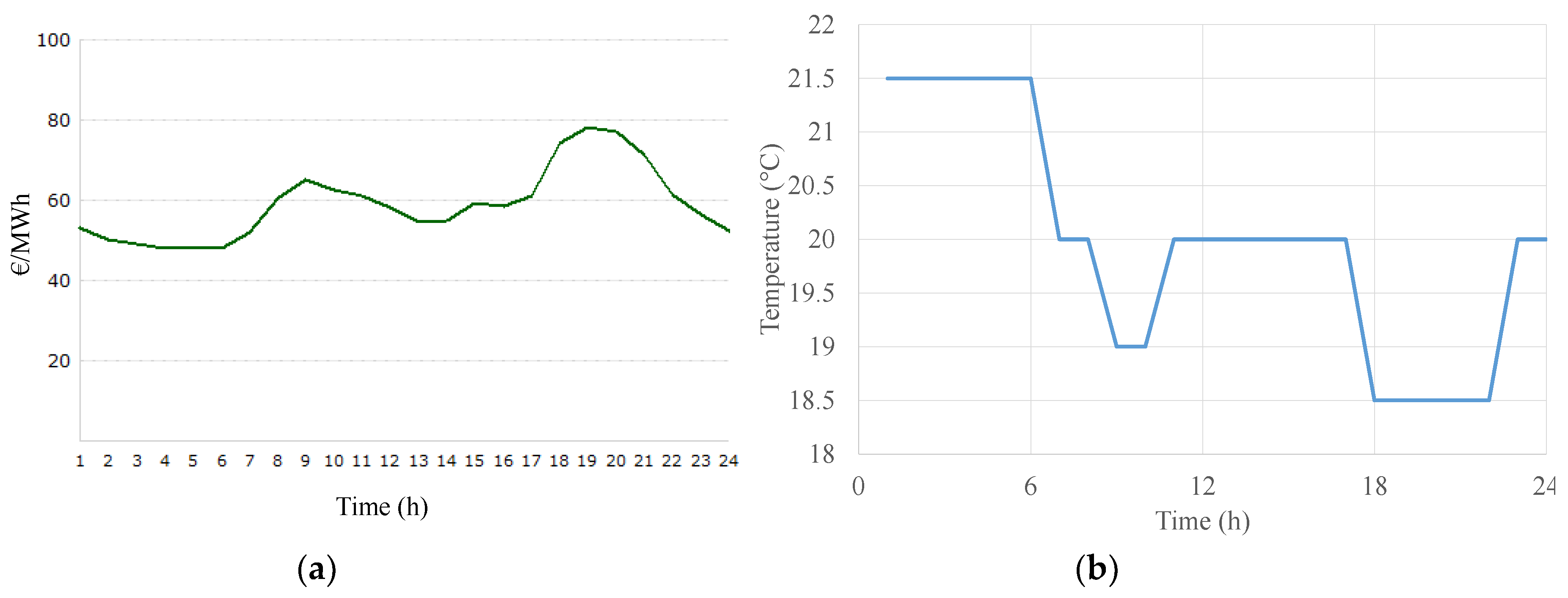
This case study considered a single dwelling of 100 m2 with an air source heat pump and underfloor heating system (Figure 2c). The heat pump capacity has been assessed at 2 kW, evaluated as 70% of the design value at the design outside temperature of −1 °C and inside temperature of 20 °C, similar to the case in Section 3.2.1. Given the thermal inertia of the chosen emission system, a storage tank is not necessary in this configuration [33]. The heat pump was controlled by the external ambient temperature (<15 °C), the indoor air temperature, and the slab surface temperature, while a minimum time of 6 min was guaranteed between any on-off cycle. The analysis aimed at showing the influence of the price signal on the HP load profile and consequently on the energy bill for the final user. When the DR strategy is applied, the final user is subject to a variable price and the system is allowed to extend the comfort band of ±2 °C. On the basis of the electricity market price on a typical winter’s day in Italy (2 January 2017 [64]), the temperature set-point was varied according to Figure 3: when the electricity market price was lower the temperature set-point was increased, when the electricity market price was higher the set-point was decreased, so to force pre-heating when the electricity is cheaper. The temperature set-point profile is a step curve which drives a rule based control (considering the thermal inertia of the considered system and the real implementation constraints for stable operation, a continuous variability of the set-point has been considered not useful).
4. Results and Discussion
4.1. Case A
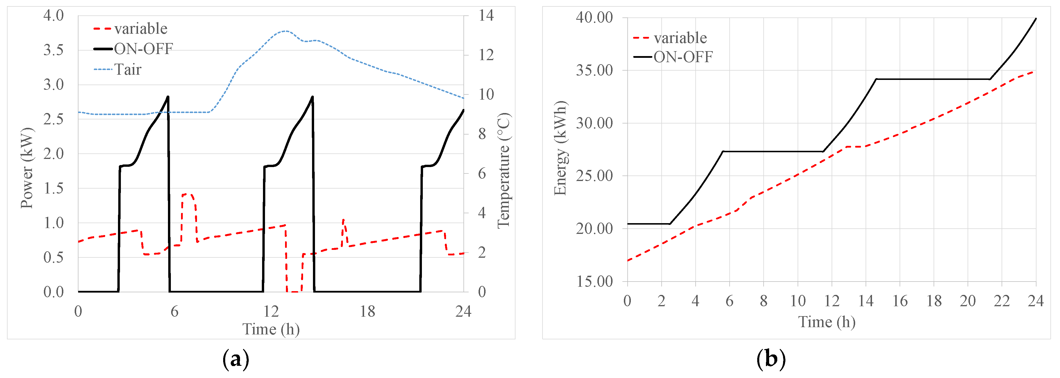
In Figure 4, the heat pump electric power consumption in case of ON-OFF operation and variable capacity is shown. It is possible to see that in the ON-OFF configuration the HP power demand is higher and the device has to cycle several times. In the variable capacity configuration, the heating load can be adjusted on the basis of the real building heat demand that varies with the external ambient temperature. During the 24 h of operation represented in Figure 4a, indeed, the ambient temperature is always higher than the design value, then the HP modulates the thermal power provided. The variable capacity heat pump allows energy savings because the energy is produced following the real demand, then reducing the need to store it and the consequent thermal losses. For instance, in the month of January, an energy use reduction of about 15% is obtained for the considered case simulated in TRNSYS. It is worth noticing that such energy saving is guaranteed even if in the variable capacity heat pump system, the auxiliaries (e.g., circulation pumps) run for longer periods.
Figure 4b, instead, represents the cumulative energy use of the heat pump in the two configurations. In case of an ON-OFF regulation, the heat pump tends to concentrate the heating of the building in given amounts of time (i.e., pre-heating) and this confirms the higher energy thermal losses. The horizontal distance between the two curves of the cumulative energy represents the time shift of the energy use, which can also reach 8 h in the case represented in Figure 4b.
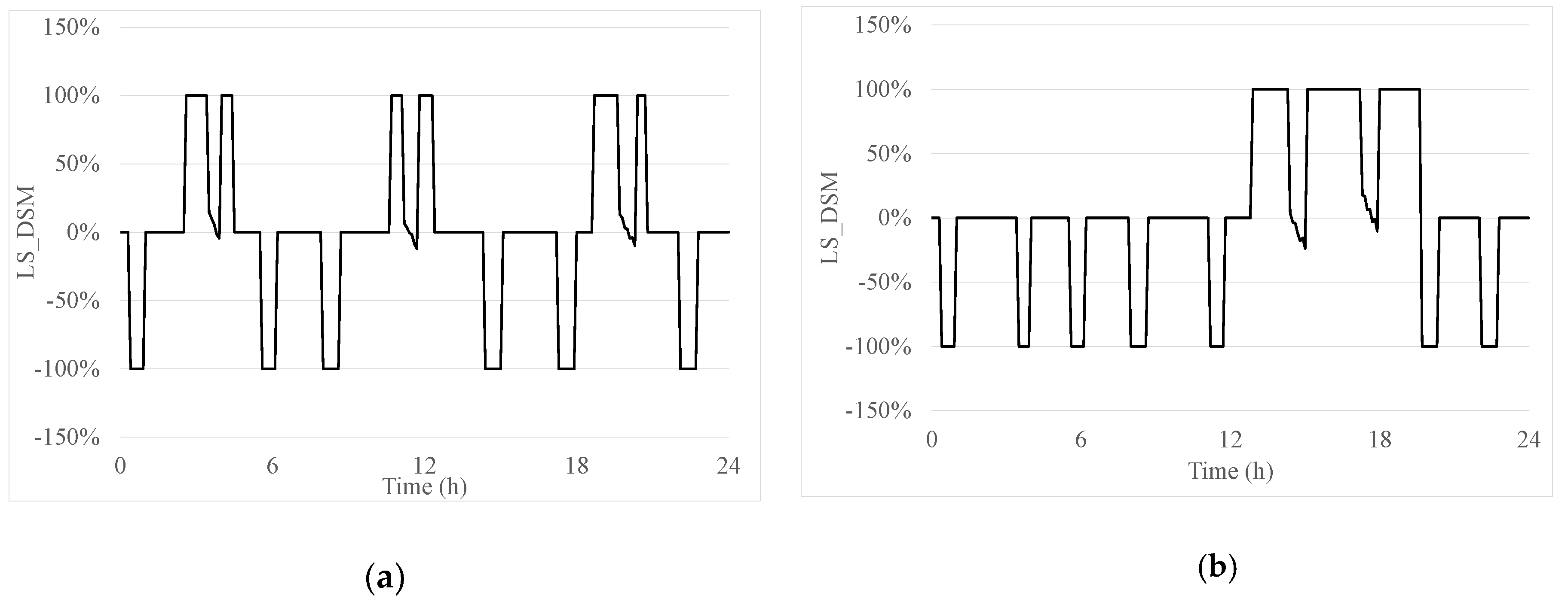
The load shifting indicator (LSDSM,t) comparing the two configurations has been calculated. It is illustrated in Figure 5. As previously explained, the variable capacity HP stays on for a longer period of time with a lower power demand. This is shown also by the load shifting indicator: it is positive when the power is higher in the variable capacity configuration and negative when it is higher in the ON-OFF configuration. It has been calculated by means of Equation (2) and set at +100% when the variable capacity HP is on, while the ON-OFF HP is off. The electric power profile modification obtained with this energy efficient action is useful, for example, for peak shaving DSM strategies: the load can be reduced to 50% or even more. Moreover, in general, energy efficient solutions help energy conservation DSM strategies.
4.2. Case B
In Figure 6a the power consumption of the heat pump, by varying the TES size, is shown. The volume varies from a small buffer tank of 20 L up to 300 L. It is apparent that by decreasing the size of the water tank, the heat pump has to switch ON/OFF several times in order to satisfy the thermal energy demand of the building. A bigger tank indeed provides more energy autonomy, and then flexibility. Figure 6a highlights also that for proper operation of the heat pump system, a minimum tank volume of 100 L is preferable, then it is considered as a reference design configuration (i.e., without DSM). Figure 6b shows the cumulative energy curves of the heat pump in the reference configuration with a tank volume of 100 L and in the “DSM configuration” with a bigger storage tank of 300 L. It is evident that the system with a higher volume tends to pre-heat more and provides energy to the house for a longer period before the heat pump needs to be switched on again. Indeed, a 100 L and 300 L can provide, respectively, 1 kWh and 3 kWh of energy stored. The time shift between the two is about 2–4 h. Regarding the total energy use, there is not a consistent difference between the two selected tank volumes. However, the energy use tends to increase with the tank size because of more energy losses during the energy storage period.
In Figure 7a the load shifting indicator is drawn when the tank size is increased from 100 L up to 300 L for 24 h of operation. Using a bigger tank, the heat pump switches on a few times for longer periods with a similar power demand in the two configurations. This solution is good for concentrating the heat pump working period in a given moment during the day, or for avoiding the operation in certain hours, for example, for night load shifting. In the latter case a bigger volume than those analyzed is needed. This is confirmed by Figure 7b which shows the load shifting indicator for a 1000 L tank compared to a 100 L tank. The HP can indeed be OFF for a long time period.
4.3. Case C
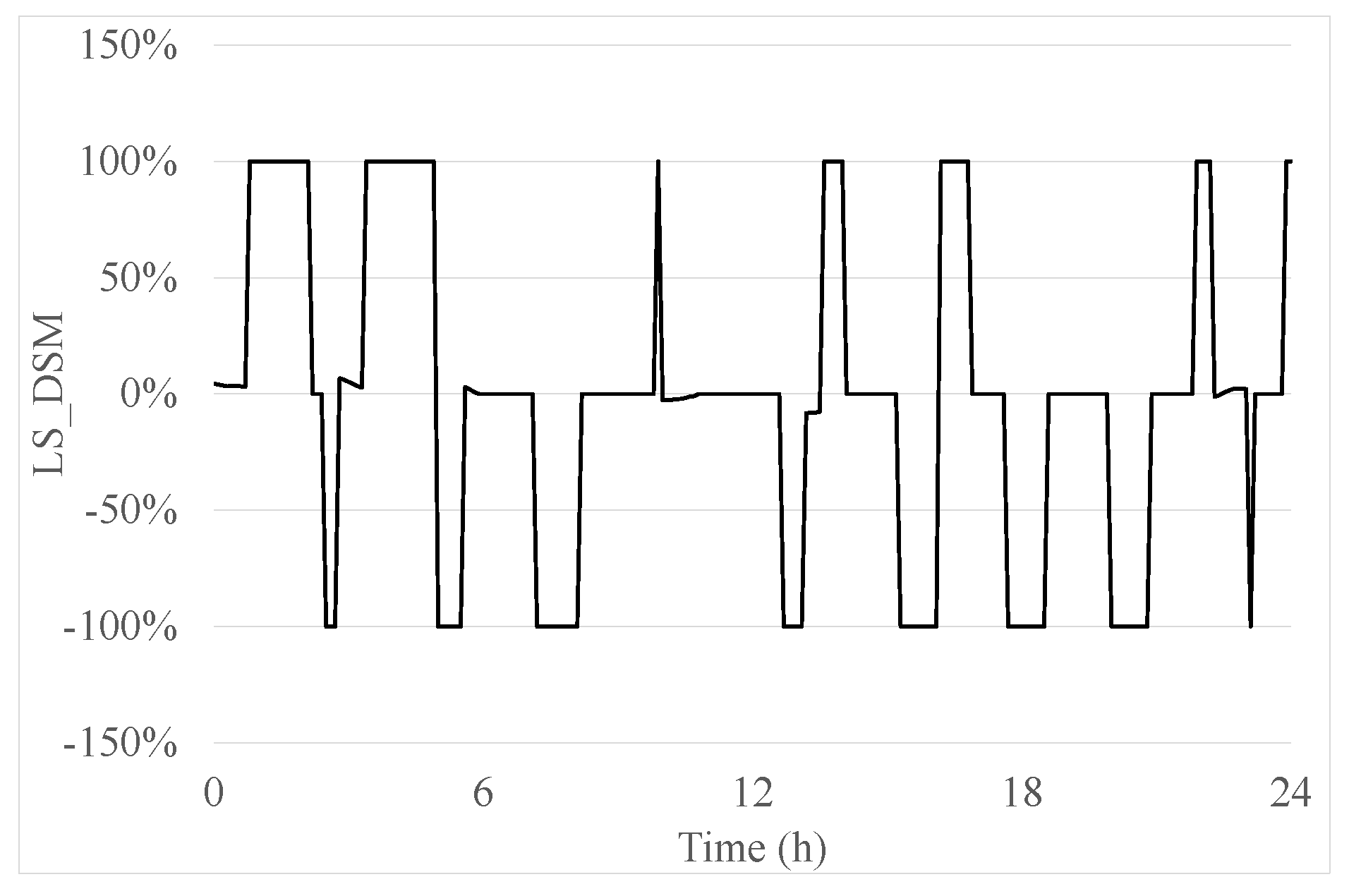
In Figure 8a the power consumption trend of the heat pump is shown for the case without DR and for the case with DR activated. It is clear that when there is a variable temperature set-point, the heat pump switches on when the latter has higher values, that is, especially during the period 0–6 h. Instead, when the temperature set-point is decreased, the heat pump tends to work for shorter periods of time. The cumulative energy curve (Figure 8b) shows that during demand response programs, the heat pump pre-heats the house and for this reason more energy is used (about 2% for the month of January). The time shift allowed can reach up to 10 h and it represents energy use in advance rather than the reference case.
Figure 9 shows the load shifting indicator when the DR program is on or off during 24 h of operation on a winter’s day. Comparing the load shifting trend with the internal temperature set-point, it is evident that the load is shifted to the hours when the set-point is higher, that is, the hours with cheaper electricity prices. Therefore, this DSM technology increases the load during off-peak hours, while decreasing it during on-peak hours.
4.4. Discussion
The presented case studies were intended to show the flexibility introduced by specific DSM technologies, namely:
- energy efficient devices, represented by a more efficient variable capacity heat pump,
- thermal storage, where different tank volumes are coupled with HP and radiators,
- demand response, implemented by means of a variable internal temperature set-point which reflects a variable electricity price.
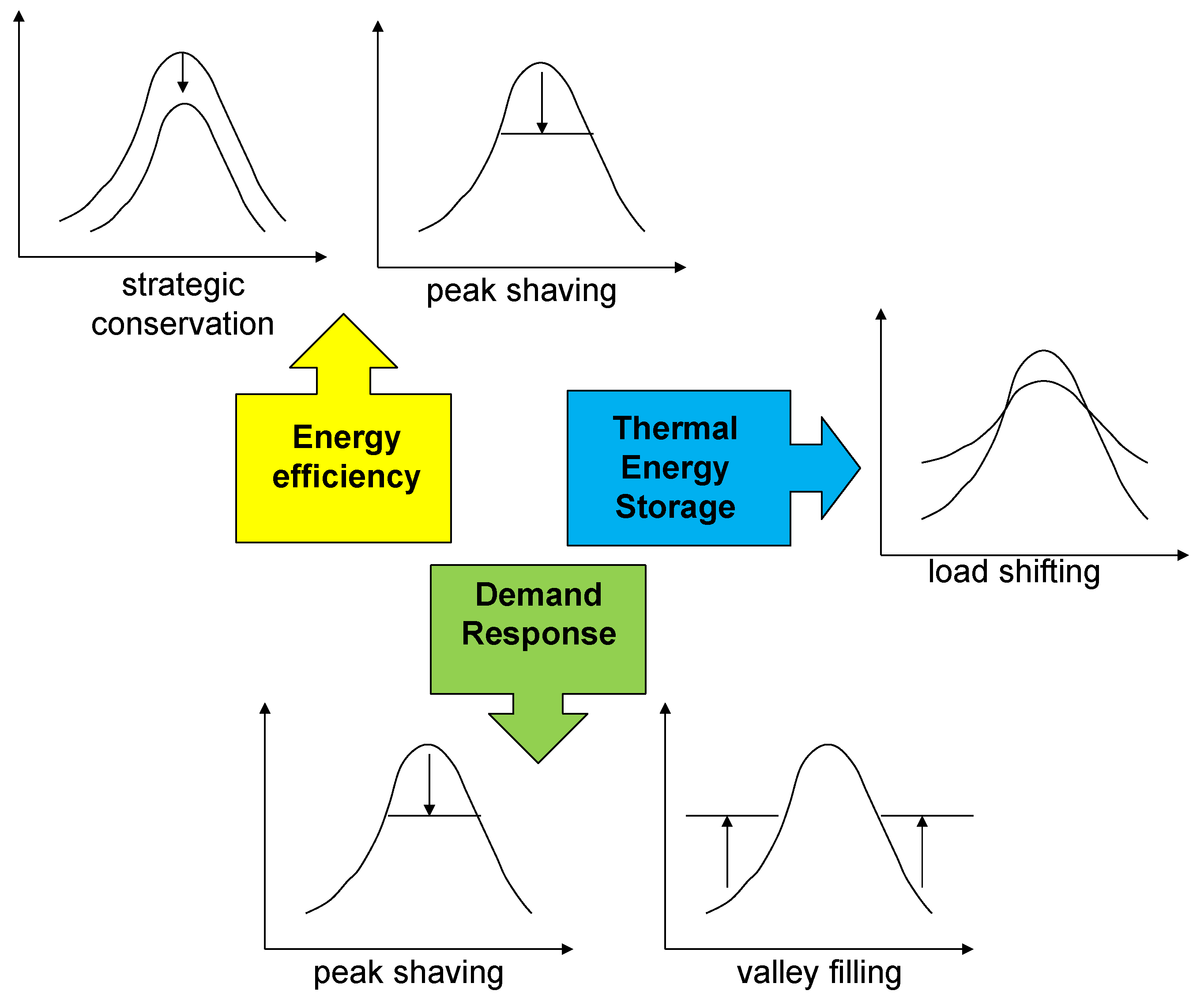
It is evident that each of these systems produces a modification of the electric power demand of the HP and provides flexibility. In more detail, looking at the HP power profile and at the LSDSM indicator, the following conclusions can be drawn (see Figure 10):
- Energy efficient DSM technologies allow energy conservation (reduction of the overall load) and, as a consequence, peak shaving (reduction of the maximum load). Indeed, the variable capacity HP is ON for longer periods but with a lower load.
- Energy storage systems achieve load shifting, and the time shifting depends on the amount of energy that can be stored. Without any other external constraints, the storage volume affects the operation of the system and the time to which the load is shifted.
- Eventually DR programs, based on real time pricing, use the price signal to induce the user to shift their load to hours with a lower electricity price. With DR programs, load shifting to off-peak hours (valley filling, i.e., building off-peak loads) and consequently peak shaving of the overall power system can be operated.
The results also clarify the role of the thermal inertia available in the considered systems. The design and configuration of the analyzed cases have a huge impact on the final results. In particular, the thermal inertia provided by the building and emission system play a major role. When an underfloor heating system is used, and without any additional energy storage tanks, the time shifting in energy use is consistent. In Case A it can reach 8 h and represents a postponed use of energy, while in Case C it goes up to 10 h of energy used in advance, rather than the reference case. Looking at the load shifting indicator, in Case A the HP load is almost always present, even if with lower values (50% of the case without DSM technology or even lower). Whereas, by comparing Case B and C, in both cases the HP is ON less times for longer periods without reduction of the peak load. The difference between the two configurations is that in Case C, the periods when the HP works are actively controlled by the electricity price (the energy use occurs more during off-peak periods), while in Case B, unless in presence of external constraints, the load shifting depends only on the size of the tank and can occur at any time, depending on the operation of the system. For the configurations analyzed, for example, with the 300 L storage tank, the heat pump switches on three times in a day for 6 h in total, instead of four times for 4 h. Furthermore, even if the configuration with radiators and TES provides a shorter time shifting potential rather than the other systems, the relative power that can be actually shifted is big (always 100%). Eventually only Case A shows a potential energy use reduction, mainly due to the fact that when energy demand is shifted in time (i.e., Case B and Case C), it needs to be stored somehow thus increasing the energy losses.
In conclusion, the LSDSM indicator provides knowledge about the dynamic behavior of a system where a considered DSM technology has been introduced. Its trends suggest the purpose of the DSM strategy (i.e., peak shaving, valley filling) and the time shifting indicator gives an idea about how much time is possible to deviate from the normal operation. The results discussed here are useful to understand the flexibility that can be expected by heat pumps in buildings and how it can be activated. These results are case specific and are related to the operation of the analyzed system: the flexibility available varies with time and is affected by what happened in the previous periods. Having similar indicators for a wide spread of technologies would allow quantifying the total flexibility that a given sector (e.g., TCL sector) can guarantee to the grid. However, in order to really understand how the flexibility can be exploited, it is necessary to model the dynamics of the overall power system with both the electricity demand side and production side. Only in this way is it possible to account for the interaction between the demand and the supply of electricity [65]. Such interaction is, for example, responsible for the payback load effect that could cause a new peak demand after a DR event or for the fact that the actual flexibility asked of every user is generally much lower than the total flexibility that the user could provide [47]. Indeed, the desynchronization and wide share of DSM events is paramount for an effective outcome for these technologies.
5. Conclusions
In this work, an overview of the demand side management strategies that can be implemented in the field of air conditioning and heat pumps is presented. The different DSM available technologies have been categorized into three groups: energy efficient devices, energy storage, and DR. In particular in this work, DSM strategies applied to heating systems using heat pumps are studied in detail in order to provide a qualitative quantification of the available flexibility and the expected behavior of such systems. Possible ways to assess the energy flexibility provided by heat pumps adhering to DSM strategies are discussed by means of three representative case studies. The flexibility is evaluated in terms of load shifting potential and time shifting of the energy use. The case studies consider the flexibility provided by: a heat pump efficient design (variable capacity HP), a thermal energy storage (thermally stratified water tank), and a DR program to drive the electricity consumptions towards off-peak hours. All the analyzed DSM technologies are effective, but they produce different effects on the basis of the system configuration. The main conclusions that can be drawn on the basis of the presented results are:
- Energy efficiency actions can produce mainly peak shaving and energy conservation. When such action is represented by a variable capacity heat pump, the load is always present but with lower values (50% or even less). In case of distribution systems with a high thermal inertia, such as underfloor heating, the energy use can be postponed for several hours (8 h in the analyzed case).
- Energy storage systems allow load shifting. The amount of energy that can be shifted depends on the storage size and, unless in presence of external constraints, the time to which the load is moved cannot be actively controlled. The time shifting in cases of low thermal inertia distribution systems, that is, radiators, is limited but the relative power that can be postponed is high (100% of the nominal value).
- DR operates an active load shifting to off-peak hours (valley filling) and peak shaving. In this case, energy is used in advance in comparison with the reference case. The time shifting is long in the presence of underfloor heating systems (for a 100 m2 apartment it can be anticipated at 4 h). This kind of strategy tends to increase the overall energy consumption but allows a better operation of the power system avoiding high peak demand.
Author Contributions
Conceptualization and Writing-Original Draft Preparation, A.A.; Writing-Review & Editing, F.P.
Funding
This research was funded by MIUR of Italy in the framework of PRIN2015 project: “Clean heating and cooling technologies for an energy efficient smart grid”, Prot. 2015M8S2PA.
Acknowledgments
The authors wish to thank the MIUR of Italy for supporting this study in the framework of PRIN2015 project: “Clean heating and cooling technologies for an energy efficient smart grid”, Prot. 2015M8S2PA
Conflicts of Interest
The authors declare no conflict of interest. The funders had no role in the design of the study; in the collection, analyses, or interpretation of data; in the writing of the manuscript, or in the decision to publish the results.
References and Note
- EIA (Energy Information Administration). How Much Energy is Consumed in Residential and Commercial Buildings in the United States? Available online: http://www.eia.gov/tools/faqs/faq.cfm?id=86&t=1 (accessed on 13 July 2018).
- EU (European Union). Energy Efficiency-Buildings. Available online: https://ec.europa.eu/energy/en/topics/energy-efficiency/buildings (accessed on 13 July 2018).
- Coulomb, D.; Dupont, J.L.; Pichard, A. The Role of Refrigeration Industry in the Global Economy; Report No. 29th Informatory Note on Refrigeration Technology; International Institute of Refrigeration: Paris, France, November, 2015. [Google Scholar]
- Thomas, N.; Pascal, W. European Heat Pump Market and Statistics Report 2015; Technical Report for The European Heat Pump Association AISBL (EHPA): Brussels, Belgium, 2015. [Google Scholar]
- Callaway, D.S.; Hiskens, I.A. Achieving controllability of electric loads. Proc. IEEE 2011, 99, 184–199. [Google Scholar] [CrossRef]
- Jensen, S.Ø.; Marszal-Pomianowska, A.; Lollini, R.; Pasut, W.; Knotzer, A.; Engelmann, P.; Stafford, A.; Reynders, G. IEA EBC Annex 67 Energy Flexible Buildings. Energy Build. 2017, 155, 25–34. [Google Scholar] [CrossRef] [Green Version]
- EU (European Union). Directive 2010/31/EU of the European Parliament and of the Council of 19 May 2010 on the Energy Performance of Buildings, 2010. Available online: https://eur-lex.europa.eu/legal-content/EN/TXT/PDF/?uri=CELEX:32010L0031&from=en (accessed on 13 July 2018).
- Strbac, G. Demand side management: Benefits and challenges. Energy Policy 2008, 36, 4419–4426. [Google Scholar] [CrossRef]
- Gellings, C.W. The smart grid. In Enabling Energy Efficiency and Demand Response; The Fairmont Press: Lilburn, GA, USA, 2009. [Google Scholar]
- Harby, K. Hydrocarbons and their mixtures as alternatives to environmental unfriendly halogenated refrigerants: An updated overview. Renew. Sustain. Energy Rev. 2017, 73, 1247–1264. [Google Scholar] [CrossRef]
- Bolajian, B.O.; Huan, Z. Ozone depletion and global warming: Case for the use of natural refrigerant—A review. Renew. Sustain. Energy Rev. 2013, 18, 49–54. [Google Scholar] [CrossRef]
- Nawaz, K.; Shen, B.; Elatar, A.; Baxter, V.; Abdelaziz, O. R290 (propane) and R600a (isobutane) as natural refrigerants for residential heat pump water heaters. Appl. Therm. Eng. 2017, 127, 870–883. [Google Scholar] [CrossRef]
- Zajacs, A.; Lalovs, A.; Borodinecs, A.; Bogdanovics, R. Small ammonia heat pumps for space and hot tap water heating. Energy Procedia 2017, 122, 74–79. [Google Scholar] [CrossRef]
- Krishnamoorthy, S.; Modera, M.; Harrington, C. Efficiency optimization of a variable-capacity/variable-blower-speed residential heat-pump system with ductwork. Energy Build. 2017, 150, 294–306. [Google Scholar] [CrossRef]
- Park, D.Y.; Yun, G.; Kim, K.S. Experimental evaluation and simulation of a variable refrigerant-flow (VRF) air-conditioning system with outdoor air processing unit. Energy Build. 2017, 146, 122–140. [Google Scholar] [CrossRef]
- Aynur, T.N.; Hwang, Y.; Radermacher, R. Simulation comparison of VAV and VRF air conditioning systems in an existing building for the cooling season. Energy Build. 2009, 41, 1143–1150. [Google Scholar] [CrossRef]
- Özahi, E.; Abusoglu, A.; Kutlar, A.I.; Dagcı, O. A comparative thermodynamic and economic analysis and assessment of a conventional HVAC and a VRF system in a social and cultural center building. Energy Build. 2017, 140, 196–209. [Google Scholar] [CrossRef]
- Sumeru, K.; Nasution, H.; Ani, F.N. A Review on two-phase ejector as an expansion device in vapor compression refrigeration cycle. Renew. Sustain. Energy Rev. 2012, 16, 4927–4937. [Google Scholar] [CrossRef]
- Wang, H.; Cai, W.; Wang, Y. Optimization of a hybrid ejector air conditioning system with PSOGA. Appl. Therm. Eng. 2017, 112, 1474–1486. [Google Scholar] [CrossRef]
- Boccardi, G.; Botticella, F.; Lillo, G.; Mastrullo, R.; Mauro, A.W.; Trinchieri, R. Experimental investigation on the performance of a transcritical CO2 heat pump with multiejector expansion system. Int. J. Refrig. 2017, 82, 389–400. [Google Scholar] [CrossRef]
- Bansal, P.; Vineyard, E.; Abdelaziz, O. Status of not-in-kind refrigeration technologies for household space conditioning, water heating and food refrigeration. Int. J. Sustain. Built Environ. 2012, 1, 85–101. [Google Scholar] [CrossRef]
- Kitanovski, A.; Egolf, P.W. Application of magnetic refrigeration and its assessment. J. Magn. Magn. Mater. 2009, 321, 777–781. [Google Scholar] [CrossRef]
- Promoppatum, P.; Yao, S.-C.; Hultz, T.; Agee, D. Experimental and numerical investigation of the cross-flow PCM heat exchanger for the energy saving of building HVAC. Energy Build. 2017, 138, 468–478. [Google Scholar] [CrossRef]
- Du, Z.; Jin, X.; Fang, X.; Fan, B. A dual-benchmark based energy analysis method to evaluate control strategies for building HVAC systems. Appl. Energy 2016, 183, 700–714. [Google Scholar] [CrossRef]
- Ascione, F.; Bianco, N.; De Stasio, C.; Mauro, G.M.; Vanoli, G.P. A new comprehensive approach for cost-optimal building design integrated with the multi-objective model predictive control of HVAC systems. Sustain. Cities Soc. 2017, 31, 136–150. [Google Scholar] [CrossRef]
- Kusiak, A.; Li, M.; Tang, F. Modeling and optimization of HVAC energy consumption. Appl. Energy 2010, 87, 3092–3102. [Google Scholar]
- Kusiak, A.; Tang, F.; Xu, G. Multi-objective optimization of HVAC system with an evolutionary computation algorithm. Energy 2011, 36, 2440–2449. [Google Scholar] [CrossRef]
- Garnier, A.; Eynard, J.; Caussanel, M.; Grieu, S. Predictive control of multizone heating, ventilation and air-conditioning systems in non-residential buildings. Appl. Soft Comput. 2015, 37, 847–862. [Google Scholar] [CrossRef] [Green Version]
- Arteconi, A.; Hewitt, N.J.; Polonara, F. State of the art of thermal storage for demand side management. Appl. Energy 2012, 93, 371–389. [Google Scholar] [CrossRef]
- Arteconi, A.; Polonara, F. Demand side management in refrigeration applications. Int. J. Heat Technol. 2017, 35, S58–S63. [Google Scholar] [CrossRef]
- Dincer, I.; Rosen, M.A. Thermal Energy Storage. Systems and Applications, 2nd ed.; Wiley: Chichester, UK, 2011. [Google Scholar]
- Hasnain, S.M. Review on sustainable thermal energy storage technologies, Part 2: Cool thermal storage. Energy Convers. Manag. 1998, 39, 1139–1153. [Google Scholar] [CrossRef]
- Arteconi, A.; Hewitt, N.J.; Polonara, F. Domestic Demand-Side Management (DSM): Role of Heat Pumps and Thermal Energy Storage (TES) systems. Appl. Therm. Eng. 2013, 51, 155–165. [Google Scholar] [CrossRef]
- Zhang, Y.; Zhou, G.; Lin, K.; Zhang, Q.; Di, H. Application of latent heat thermal energy storage in buildings: State-of-the-art and outlook. Build. Environ. 2007, 42, 2197–2209. [Google Scholar] [CrossRef]
- Arteconi, A.; Costola, D.; Hoes, P.; Hensen, J.L.M. Analysis of control strategies for thermally activated building systems under demand side management mechanisms. Energy Build. 2014, 80, 384–393. [Google Scholar] [CrossRef] [Green Version]
- Yin, R.; Kara, E.C.; Li, Y.; DeForest, N.; Wang, K.; Yong, T.; Stadler, M. Quantifying flexibility of commercial and residential loads for demand response using setpoint changes. Appl. Energy 2016, 177, 149–164. [Google Scholar] [CrossRef] [Green Version]
- Fischer, D.; Madani, H. On heat pumps in smart grids: A review. Renew. Sustain. Energy Rev. 2017, 70, 342–357. [Google Scholar] [CrossRef]
- Geidl, M.; Arnoux, B.; Plaisted, T.; Dufour, S. A fully operational virtual energy storage network providing flexibility for the power system. In Proceedings of the 12th IEA Heat Pump Conference, Rotterdam, The Netherlands, 15–18 May 2017. [Google Scholar]
- Schwalbea, R.; Häuslerb, M.; Stiftera, M.; Esterl, T. Market driven vs. grid supporting heat pump operation in low voltage distribution grids with high heat pump penetration—An Austrian case study. In Proceedings of the 12th IEA Heat Pump Conference, Rotterdam, The Netherlands, 15–18 May 2017. [Google Scholar]
- Bruninx, K. Improved Modeling of Unit Commitment Decisions under Uncertainty. Ph.D. Thesis, KU Leuven, Leuven, Belgium, 2016. [Google Scholar]
- Rahmani-Andebili, M. Modeling nonlinear incentive-based and price-based demand response programs and implementing on real power markets. Electr. Power Syst. Res. 2016, 132, 115–124. [Google Scholar] [CrossRef]
- Rahmani-andebili, M.; Shen, H. Energy Management of End Users Modeling their Reaction from a GENCO’s Point of View. In Proceedings of the International Conference on Computing, Networking and Communications (ICNC), Silicon Valley, San Francisco, CA, USA, 26–29 January 2017. [Google Scholar]
- Rahmani-andebili, M. Investigating Effect of Responsive Loads Models on Unit Commitment Collaborated with Demand Side Resources. IET Gener. Transm. Distrib. J. 2013, 7, 420–430. [Google Scholar] [CrossRef]
- Baetens, R.; De Coninck, R.; Van Roy, J.; Verbruggen, B.; Driesen, J.; Helsen, L.; Saelens, D. Assessing electrical bottlenecks at feeder level for residential net zero-energy buildings by integrated system simulation. Appl. Energy 2012, 96, 74–83. [Google Scholar] [CrossRef]
- Arteconi, A.; Ciarrocchi, E.; Pan, Q.; Carducci, F.; Comodi, G.; Polonara, F.; Wang, R. Thermal energy storage coupled with PV panels for demand side management of industrial building cooling loads. Appl. Energy 2016, 185, 1984–1993. [Google Scholar] [CrossRef]
- Shen, B.; Ghatikar, G.; Lei, Z.; Li, J.; Wikler, G.; Martin, P. The role of regulatory reforms, market changes, and technology development to make demand response a viable resource in meeting energy challenges. Appl. Energy 2014, 130, 814–823. [Google Scholar] [CrossRef]
- Arteconi, A.; Patteeuw, D.; Bruninx, K.; Delarue, E.; D’haeseleer, W.; Helsen, L. Active demand response with electric heating systems: Impact of market penetration. Appl. Energy 2016, 177, 636–648. [Google Scholar] [CrossRef]
- Rahmani-andebili, M. Nonlinear demand response programs for residential customers with nonlinear behavioral models. Energy Build. 2016, 119, 352–362. [Google Scholar] [CrossRef]
- Rahmani-andebili, M.; Shen, H. Price-Controlled Energy Management of Smart Homes for Maximizing Profit of a GENCO. IEEE Trans. Syst. Man Cybern. Syst. 2017. [Google Scholar] [CrossRef]
- Nuytten, T.; Claessens, B.; Paredis, K.; Van Bael, J.; Six, D. Flexibility of a combined heat and power system with thermal energy storage for district heating. Appl. Energy 2013, 104, 583–591. [Google Scholar] [CrossRef]
- D’hulst, R.; Labeeuw, W.; Beusen, B.; Claessens, S.; Deconinck, G.; Vanthournout, K. Demand response flexibility and flexibility potential of residential smart appliances: Experiences from large pilot test in Belgium. Appl. Energy 2015, 155, 79–90. [Google Scholar] [CrossRef]
- De Coninck, R.; Helsen, L. Quantification of flexibility in buildings by cost curves—Methodology and application. Appl. Energy 2016, 162, 653–665. [Google Scholar] [CrossRef]
- Oldewurtel, F.; Sturzenegger, D.; Andersson, G.; Morari, M.; Smith, R.S. Towards a standardized building assessment for demand response. In Proceedings of the IEEE Conference on Decision and Control, Firenze, Italy, 10–13 December 2013; pp. 7083–7088. [Google Scholar]
- Vanhoudt, D.; Geysen, D.; Claessens, B.; Leemans, F.; Jespers, L.; Van Bael, J. An actively controlled residential heat pump: Potential on peak shaving and maximization of self-consumption of renewable energy. Renew. Energy 2014, 63, 531–543. [Google Scholar] [CrossRef]
- Reynders, G.; Diriken, J.; Saelens, D. Generic characterization method for energy flexibility: Applied to structural thermal storage in residential buildings. Appl. Energy 2017, 198, 192–202. [Google Scholar] [CrossRef]
- Fischer, D.; Wolf, T.; Wapler, J.; Hollinger, R.; Madani, H. Model-based flexibility assessment of a residential heat pump pool. Energy 2017, 118, 853–864. [Google Scholar] [CrossRef]
- Stinner, S.; Huchtemann, K.; Müller, D. Quantifying the operational flexibility of building energy systems with thermal energy storages. Appl. Energy 2016, 181, 140–154. [Google Scholar] [CrossRef]
- Bianco, V.; Scarpa, F.; Tagliafico, L.A. Estimation of primary energy savings by using heat pumps for heating purposes in the residential sector. App. Therm. Eng. 2017, 114, 938–947. [Google Scholar] [CrossRef]
- Select Software 7, Emerson Climate Technologies. Available online: http://www.emersonclimate.com/europe/en-eu/Resources/Software_Tools/Pages/Download_Full_Instructions.aspx (accessed on 13 July 2018).
- Klein, S.A.; Beckman, W.A.; Mitchel, J.W.; Duffie, J.A.; Duffie, N.A.; Freeman, T.L. TRNSYS Manual; University of Wisconsin-Madison: Madison, WI, USA, 2009. [Google Scholar]
- Salvala, G.; Pfafferott, J.; Jacob, D. Validation of a low-energy whole building simulation model. Proc. SimBuild 2010, 4, 32–39. [Google Scholar]
- Ballarini, I.; Corgnati, S.P.; Corrado, V. Use of reference buildings to assess the energy saving potentials of the residential building stock: The experience of TABULA project. Energy Policy 2014, 68, 273–284. [Google Scholar] [CrossRef]
- Italian Legislative Decree 311/2006. Disposizioni Correttive ed Integrative al Decreto Legislativo 19 Agosto 2005, n. 192, Recante Attuazione Della Direttiva 2002/91/CE, Relativa al Rendimento Energetico Nell’edilizia; Gazzetta Ufficiale Serie Generale n.26 del 01-02-2007 - Suppl. Ordinario n. 26, Roma, Italy, 2007.
- Gestore del Mercato Elettrico. Available online: http://www.mercatoelettrico.org/it/ (accessed on 13 July 2018).
- Patteeuw, D.; Bruninx, K.; Arteconi, A.; Delarue, E.; D’haeseleer, W.; Helsen, L. Integrated modeling of active demand response with electric heating systems coupled to thermal energy storage systems. Appl. Energy 2015, 151, 306–319. [Google Scholar] [CrossRef] [Green Version]
Figure 1.
Cold thermal energy storage (CTES) operational strategies [29,30]. (A) A full storage strategy shifts the entire peak cooling load to off-peak hours. In a partial storage strategy, the load is partially supplied by the thermal storage and partially by the refrigeration unit. The chiller can be designed to operate as (B) load levelling or (C) demand limiting.

Figure 2.
Schematics of the three case studies: (a) Case A: energy efficiency, (b) Case B: thermal storage, (c) Case C: demand response. TES = thermal energy storage; DR = demand response.
Figure 2.
Schematics of the three case studies: (a) Case A: energy efficiency, (b) Case B: thermal storage, (c) Case C: demand response. TES = thermal energy storage; DR = demand response.
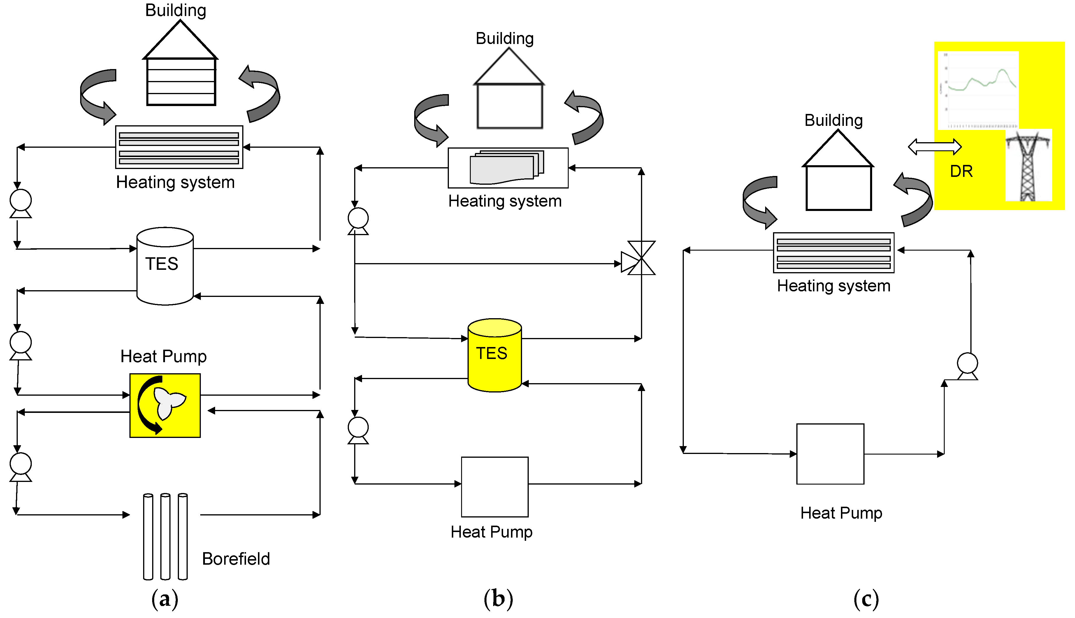
Figure 3.
(a) Electricity market price on a winter’s day (2 January 2017) and (b) daily internal temperature set-point profile.
Figure 3.
(a) Electricity market price on a winter’s day (2 January 2017) and (b) daily internal temperature set-point profile.

Figure 4.
(a) Electric power profile and (b) cumulative energy curve of the heat pump (HP) in ON-OFF configuration and variable capacity configuration.
Figure 4.
(a) Electric power profile and (b) cumulative energy curve of the heat pump (HP) in ON-OFF configuration and variable capacity configuration.

Figure 5.
Load shifting indicator (LSDSM,t) for a typical winter’s day: comparison between the two configurations with (variable capacity HP) and without demand side management (DSM) (ON-OFF HP).
Figure 5.
Load shifting indicator (LSDSM,t) for a typical winter’s day: comparison between the two configurations with (variable capacity HP) and without demand side management (DSM) (ON-OFF HP).
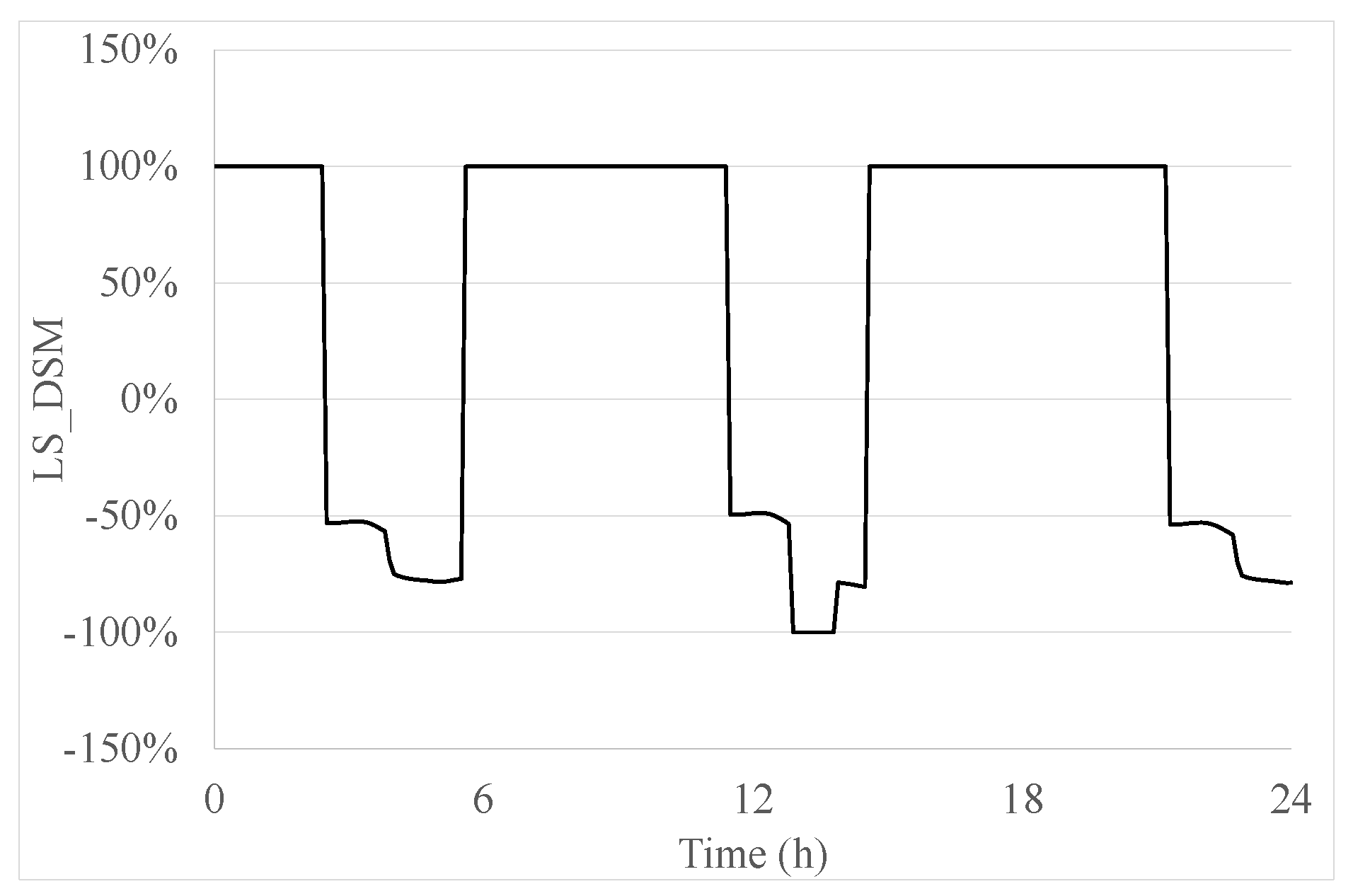
Figure 6.
(a) Electric power profile and (b) cumulative energy curve of the HP for different tank sizes.
Figure 6.
(a) Electric power profile and (b) cumulative energy curve of the HP for different tank sizes.
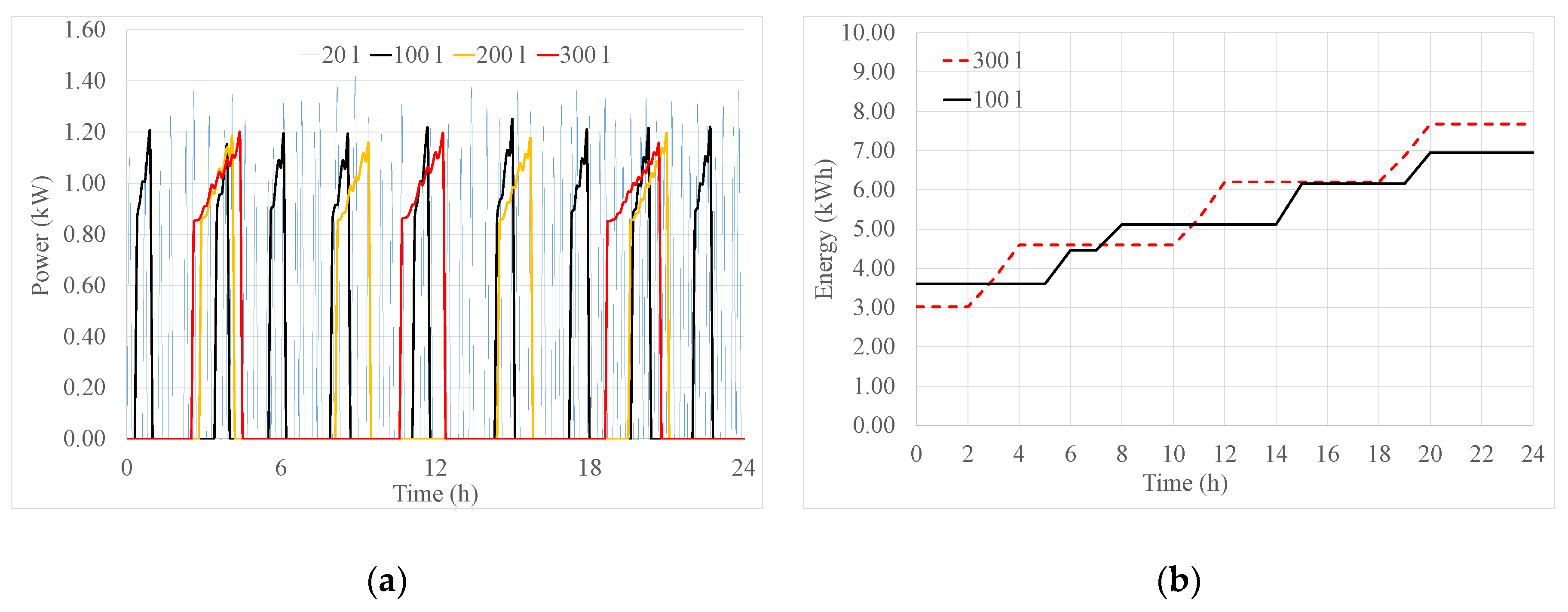
Figure 7.
Load shifting indicator (LSDSM,t).for the comparison between (a) a system with a 300 L vs. 100 L TES and (b) a system with 1000 L vs. 100 L TES.
Figure 7.
Load shifting indicator (LSDSM,t).for the comparison between (a) a system with a 300 L vs. 100 L TES and (b) a system with 1000 L vs. 100 L TES.

Figure 8.
(a) Electric power profile and (b) cumulative energy curve of the HP with and without the DR program.
Figure 8.
(a) Electric power profile and (b) cumulative energy curve of the HP with and without the DR program.
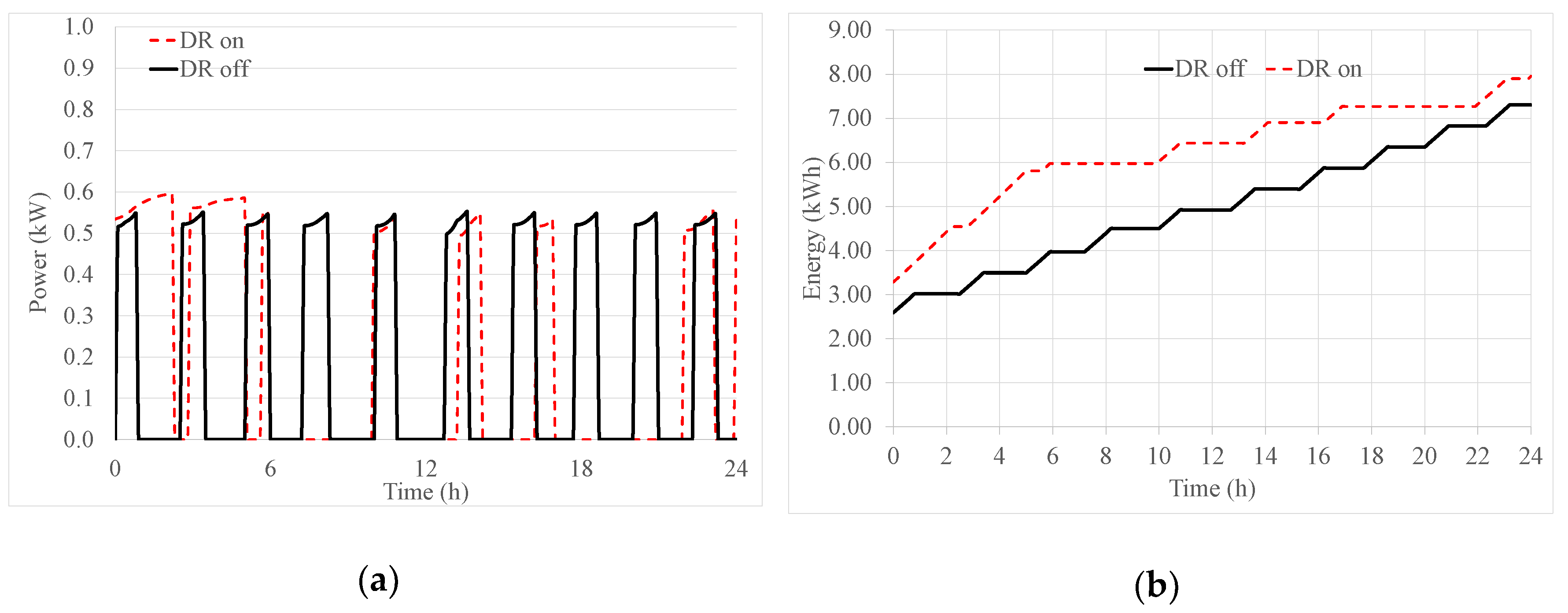
Figure 9.
Load shifting indicator (LSDSM,t) for the comparison between the system with or without the DR program.
Figure 9.
Load shifting indicator (LSDSM,t) for the comparison between the system with or without the DR program.

Figure 10.
DSM technologies and the DSM strategies that they can help to implement.


Table 1.
Summary of the demand side management (DSM) technologies implemented in the heating ventilation and air conditioning (HVAC) sector.
Table 1.
Summary of the demand side management (DSM) technologies implemented in the heating ventilation and air conditioning (HVAC) sector.
| Category | Technology |
|---|---|
| Energy efficiency | Natural refrigerants Optimal design Not-in-kind technologies Optimal control strategies |
| Storage | Cold Thermal Energy Storage/Thermal Energy Storage Thermally Activated Buildings Phase Change Material |
| Demand Response | Ancillary services (frequency and voltage control, congestion management, spinning and non-spinning reserves) Renewable Energy Sources integration Cost reduction |
| Case | Area m2 | S/V | Windows Area % | U_Wall W/m2K | U_Roof W/m2K | U_Windows W/m2K |
|---|---|---|---|---|---|---|
| A | 1000 | 0.37 | 10 | 0.30 | 0.23 | 1.4 |
| B | 100 | 0.37 | 10 | 0.36 | 0.28 | 2.10 |
| C | 100 | 0.37 | 10 | 0.36 | 0.28 | 2.10 |
Table 3.
Design parameters of the heating system.
| Specification | Case A | Case B | Case C |
|---|---|---|---|
| Heating system | GCHP | ASHP | ASHP |
| Distribution system | floor | radiators | floor |
| Heating system supply temperature | 20–40 °C | 40–50 °C | 20–40 °C |
| HP design capacity | 8 kW | 3 kW | 2 kW |
| COPdesign | 4 | 2.5 | 3 |
| Tank volume | 1000 L | 20 L, 100 L, 200 L, 300 L, 1000 L | -- |
© 2018 by the authors. Licensee MDPI, Basel, Switzerland. This article is an open access article distributed under the terms and conditions of the Creative Commons Attribution (CC BY) license (http://creativecommons.org/licenses/by/4.0/).
Share and Cite
MDPI and ACS Style
Arteconi, A.; Polonara, F. Assessing the Demand Side Management Potential and the Energy Flexibility of Heat Pumps in Buildings. Energies 2018, 11, 1846. https://doi.org/10.3390/en11071846
AMA Style
Arteconi A, Polonara F. Assessing the Demand Side Management Potential and the Energy Flexibility of Heat Pumps in Buildings. Energies. 2018; 11(7):1846. https://doi.org/10.3390/en11071846
Chicago/Turabian StyleArteconi, Alessia, and Fabio Polonara. 2018. "Assessing the Demand Side Management Potential and the Energy Flexibility of Heat Pumps in Buildings" Energies 11, no. 7: 1846. https://doi.org/10.3390/en11071846
Note that from the first issue of 2016, this journal uses article numbers instead of page numbers. See further details here.