Six-Phase Space Vector PWM under Stator One-Phase Open-Circuit Fault Condition


College of Electrical and Information Engineering, Hunan University, Changsha 410082, China
*
Author to whom correspondence should be addressed.
Energies 2018, 11(7), 1796; https://doi.org/10.3390/en11071796
Submission received: 9 June 2018
/
Revised: 2 July 2018
/
Accepted: 4 July 2018
/
Published: 9 July 2018
Abstract
:The torque pulsation and speed pulsation of a six-phase induction machine with double Y-connected windings displaced by 30° increase after one phase of the stator winding is open-circuited. To reduce the pulsations, a method of six-phase space vector pulse width modulation (PWM) with fault-tolerance is proposed. The star point of the open-circuit winding group is connected to the centre point of the converter DC voltage. The 32 column matrices, which represent 32 stator winding voltages, are mapped to the d-q and z1-z2 planes using a new five-dimensional orthogonal matrix; then, 32 basic vectors are obtained. By using an optimal model, six auxiliary vectors and an equivalent null vector are constructed, the magnitudes of which are all zero in the z1-z2 plane. By using the auxiliary vectors and equivalent null vector, the reference vector is synthesized, the zero magnitude of which in the z1-z2 plane can suppress the harmonic voltages, and the circular trajectory of which in the d-q plane can make the torque smooth. The simulation and experimental results show that the torque pulsation range and speed pulsation range of the proposed method with fault-tolerance are 30% and 25% of those of the classical method without fault-tolerance, respectively. Thus, the phase-deficient operation performance of the system is improved.
1. Introduction
The six-phase induction machine with double Y-connected windings displaced by 30° has received considerable attention in the fields related to power drive, servo control, and new energy power generation, as well as other fields [1,2,3,4]. The stator of the machine has an asymmetric six-phase winding, where the second three-phase winding (hereafter termed BDF-winding group) is phase-advanced by 30° electrical angle with respect to the first three-phase winding (hereafter termed ACE-winding group), as shown in Figure 1a. The rotor may be a squirrel rotor or a wound-rotor. One advantage of the motor over the conventional three-phase machine is that the lower-order harmonic components of the magnetic motive force can be eliminated by using the asymmetric six-phase winding. Another advantage is that the higher power can be transmitted in the same voltage or current level condition because of the increase in number of the winding phase. The third advantage is that the machine can continuously run under phase-deficient conditions [5,6,7].
In the system composed of the machine and a six-phase two-level converter, under normal conditions, both star point m of the ACE-winding group and star point n of the BDF-winding group are electrically isolated, as shown in Figure 1a, to cut off the third and its multiple harmonic currents. With this circuit configuration, a six-phase space vector pulse width modulation (SVPWM) method is proposed in [8], which can simultaneously control the volt-second balance in three decoupling planes using the space vector decoupling theory. Therefore, the stator flux trajectory is circular, and the motor has good torque and speed.
In complex and changeable working conditions, a fault with stator one-phase open-circuit may occur in the system. Some other faults in the system can eventually be equivalent to this fault [9,10]. In this case, if the proposed method of a previous paper [8] (hereafter called the non-fault-tolerant SVPWM) is used, the stator winding voltages are out of balance, and the stator flux trajectory is no longer circular. Although the machine can run continuously, it performs poorly, e.g. the torque pulsation and speed pulsation would increase [11,12,13].
For the fault, a previous paper [14] presents an SVPWM method where two star points are interconnected; then, a five-dimensional matrix is constructed according to the equivalent principle of equal magnetic motive force and equal power before and after the coordinate transformation. Using the five-dimensional matrix, they obtain the basic voltage vectors. However, the order of the differential equation of the machine is not reduced after the transformation, and the harmonic currents are not cut off because the two star points are interconnected. Thus, the complexity and instability of the control increase. The method introduced in a previous paper [15] gives up the faulty three-phase winding group and implements the three-phase SVPWM for the healthy three-phase winding group. Although it can achieve good operation performance, it does not fully use the faulty three-phase winding group, so the capacity of the machine decreases. In addition, in a conventional or symmetric six-phase machine, the three-phase winding groups are displaced by 60°. Previous papers [16,17] investigate the SVPWM under the phase failure of this machine, and the basic characteristics are similar to those in a previous paper [14]. For the open-circuit fault of multiphase machines, current follow PWM methods are proposed in previous papers [18,19,20] to maintain the circular trajectory of the stator flux. These methods have the advantages of convenient control and fast transient response, but a disadvantage of non-constant switching frequency of the converters.
In this paper, by taking the system composed of the six-phase induction motor with double Y-connected windings displaced by 30° and the six-phase two-level inverter as study object, a method of SVPWM with fault-tolerance (hereafter termed fault-tolerant SVPWM) is proposed in order to reduce the torque pulsation and speed pulsation under stator one-phase open-circuit fault condition. Then, the correctness and effectiveness of the proposed method are verified through simulations and experiments.
2. Fault-Tolerant SVPWM
2.1. Overall Design
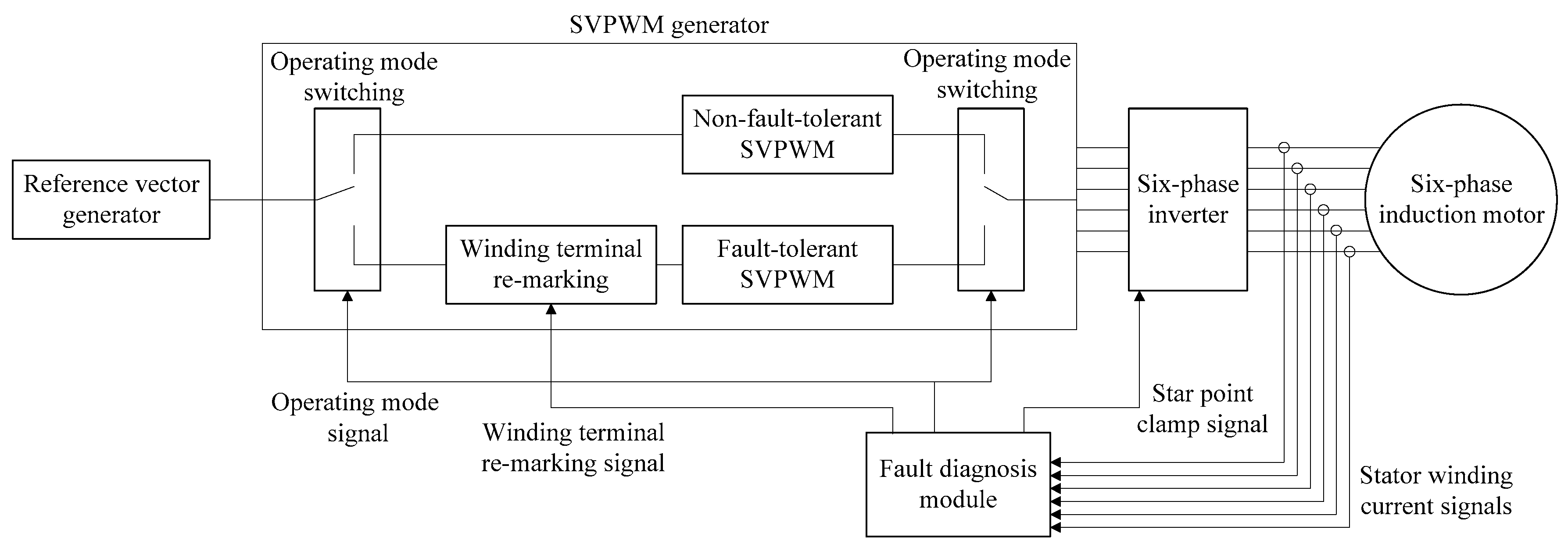
The schematic diagram of control structure is shown in Figure 2, where there are three main modules: a reference vector generator, an SVPWM generator, and a fault diagnosis module. The SVPWM generator has four function frames: the operating mode switching, the non-fault-tolerant SVPWM, the winding terminal re-marking, and the fault-tolerant SVPWM.
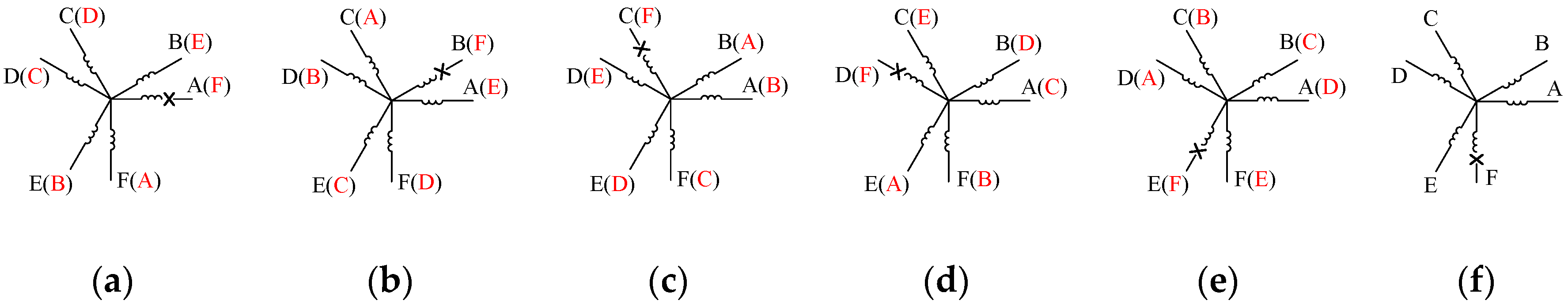
The fault diagnosis module can determine whether the six current signals of the stator winding are zero, and output three control signals: an operating mode signal, a winding terminal re-marking signal, and a star point clamp signal. The operating mode signal can control the switching of two operating modes. In this paper, simulation 1 and experiment 1 use the non-fault-tolerant SVPWM under both the normal condition and fault condition, while simulation 2 and experiment 2 use the non-fault-tolerant SVPWM under the normal condition, and use the fault-tolerant SVPWM under the fault condition. Before running the fault-tolerant SVPWM, it is necessary to remark the winding terminals, that is, to renumber the physical quantities of six windings. As shown in Figure 3, the letters in parentheses are the winding number after failures. It is known from Figure 3 that no matter which phase winding is open-circuited, it can be equivalent to the F-phase failure.
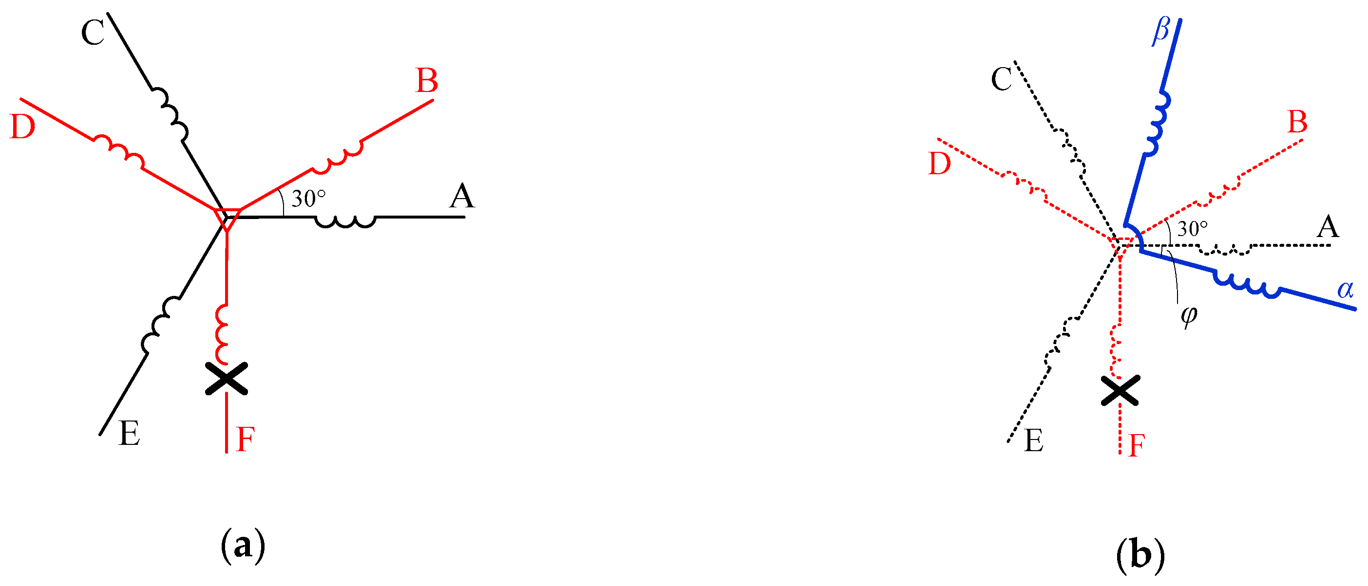
Without loss of generality and assuming that the F-phase winding is open-circuited, the current through the F-phase winding becomes zero, whereas the voltage across the F-phase winding is not zero because the induced voltage remains, which cannot be directly controlled. To control the B-phase and D-phase winding voltages, while fully using the B-phase and D-phase windings, the voltage clamp for star point n is made. As shown in Figure 1b, a triode AC switch (TRIAC) is connected between star pint n and centre point g of the inverter DC voltage, which is switched on by the star point clamp signal from the fault diagnosis module. When the F-phase winding becomes open-circuited, the TRIAC is switched on, star point n is connected to centre point g, and the potential of star point n is clamped.
2.2. Coordinate Transformation Matrix
After the F-phase winding becomes open-circuited, the stator winding can be considered an asymmetric five-phase winding, the physical model of which is shown in Figure 5a. On the basis of the dynamic mathematical model of the six-phase motor, the physical quantities related to the F-phase winding are deleted, and the F-phase-deficient dynamic mathematical model of the six- phase motor is obtained. The model requires a five-dimensional matrix to perform the coordinate transformation. The matrix should follow the equivalent principle of equal magnetic motive force and equal power before and after the transformation. The matrix that satisfies the principle is not unique; therefore, the equivalent models of the motor obtained using different matrices are identical.
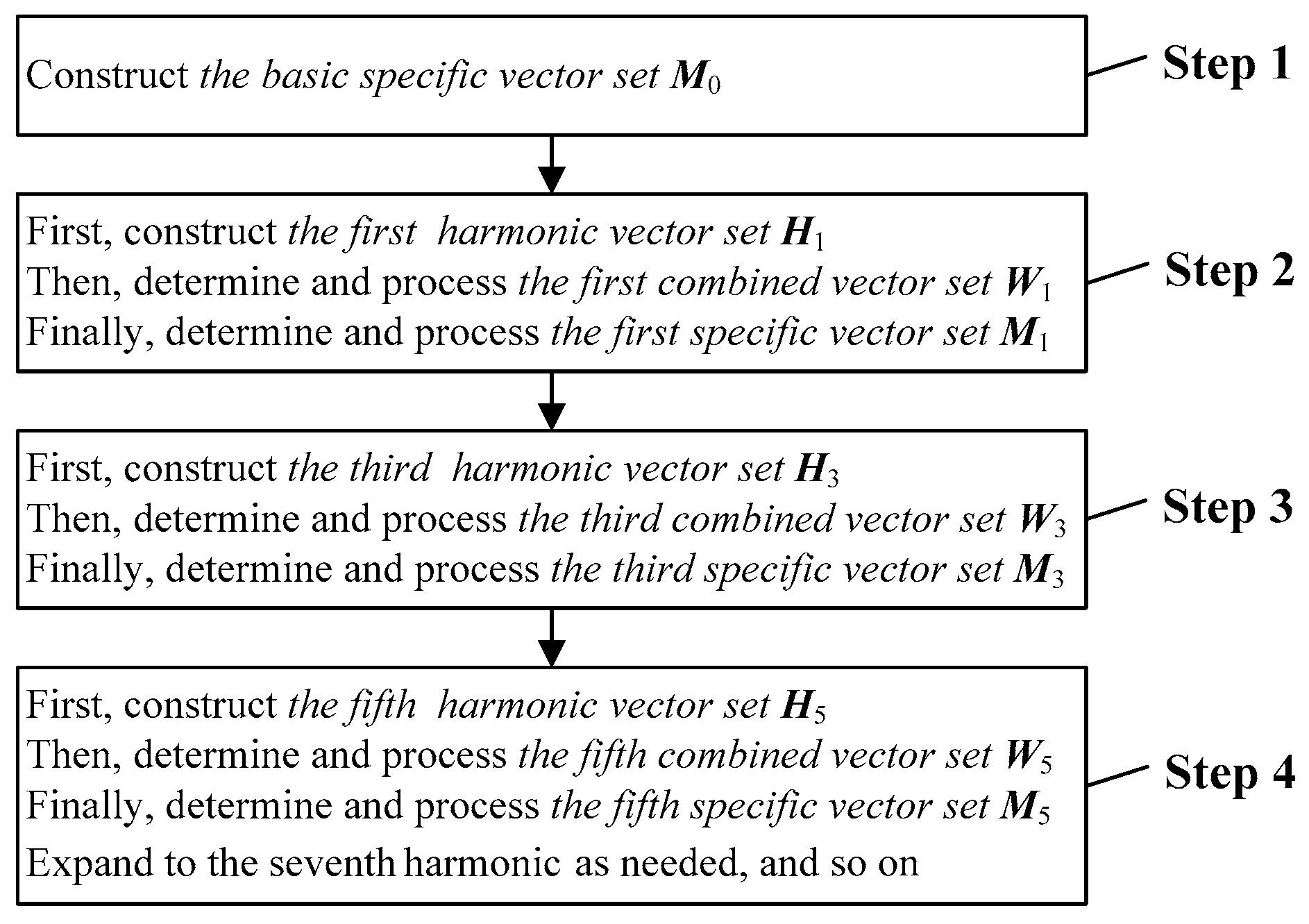
In this paper, a scheme of matrix construction is proposed, where the current constraint condition of the remaining healthy phase windings is considered in addition to the equivalent principle above. Therefore, the scheme can reduce the order of the differential equation of the motor, and be extended to arbitrary-phases open-circuit fault of multiphase machines. The detailed steps are performed according to the flow chart in Figure 6.
Step 1: Construct the basic specific vector set M0: m01, m02, … according to the current constraint condition of the remaining healthy phase windings. The number of vectors in M0 is equal to the number of current constraint conditions. Because the current constraint conditions are independent of one another, M0 is linearly independent. With the circuit configuration in Figure 1b, there is one current constraint condition: iA + iC + iE = 0; thus, one vector m01 is obtained.
m01T = [1 0 1 0 1]
Step 2: First, construct the first harmonic vector set H1: h11, h12 according to the equivalent principle of equal first magnetic motive forces before and after the transformation. H1 has two vectors: h11 and h12. For the circuit configuration in Figure 1b, establish the two-phase station reference frame (α-β) on the physical model diagram of the stator windings; the angle between the α-axis and the A-axis is ϕ, as shown in Figure 5b, and there is
Vectors h11 and h12 must satisfy h11Th12 = 0; thus, ϕ = 0 can be determined. Substituting ϕ = 0 into (2) gives
Then, combining the basic specific vector set M0 and first harmonic vector set H1 yields the first combined vector set W1. Furthermore, determine whether W1 is linearly independent. If yes, the first specific vector set M1 is obtained, which is equal to W1; if no, any one vector in M0 can be deleted from W1; then, determine whether the processed W1 is linearly independent. Here, W1 is linearly independent, so M1 = W1.
Finally, determine whether the rank of the first specific vector set M1 is equal to the number of remaining healthy phase windings. If yes, transforming M1 into an orthonormal vector set by Gram-Schmidt orthogonalization gives the desired coordinate transformation matrix; if no, proceed to the next step. Here, the rank of M1 is 3, whereas the number of remaining healthy phase windings is 5, so we proceed to the next step.
Step 3: First, construct the third harmonic vector set H3: h31, h32 according to the equivalent principle of equal third magnetic motive forces before and after the transformation. H3 has two vectors: h31, h32.
Substituting ϕ = 0 into (4) gives
Then, combining the first specific vector set M1 and third harmonic vector set H3 yields the third combined vector set W3. Furthermore, determine whether W3 is linearly independent. If yes, the third specific vector set M3 is obtained, which is equal to W3; if no, any one vector in H3 can be deleted from W3; then, determine whether the processed W3 is linearly independent. Here, W3 is not linearly independent because h31 = m01. We delete h31 from W3 to make the processed W3 become linearly independent. Thus, M3 is equal to the processed W3, which contains m01, h11, h12, and h32.
Finally, determine whether the rank of the third specific vector set M3 is equal to the number of remaining healthy phase windings. If yes, transforming M3 into an orthonormal vector set yields the desired coordinate transformation matrix; if no, proceed to the next step. Here, the rank of M3 is 4, whereas the number of remaining healthy phase windings is 5, so we proceed to the next step.
Step 4: Similar to Step 3, first construct the fifth harmonic vector set, then determine and process the fifth combined vector set, finally determine and process the fifth specific vector set. If the rank of the fifth specific vector set remains unequal to the number of remaining healthy phase windings, we continue to expand to the seventh harmonic, and so on.
Here, the extension to the fifth harmonic is performed, and the specific process is no longer detailed. The fifth specific vector set M5 contains m01, h11, h12, h32, and h51. The rank of M5 is 5, which is equal to the number of remaining health phase windings. Therefore, transforming M5 into an orthonormal vector set by Gram-Schmidt orthogonalization gives the desired coordinate transformation matrix T5×5 as follows.
where dT, qT, z1T, z2T, and z3T correspond to h11T, h12T, h32T, h51T, and m01T, respectively. For convenience, the two-dimensional space generated by dT and qT is the d-q plane, the two-dimensional space generated by z1T and z2T is the z1-z2 plane, and the one-dimensional space generated by z3T is the z3 axis.
Using (6), we perform a coordinate transformation to the F-phase-deficient dynamic mathematical model of the six-phase motor, and the stator voltage equation is as follows
where usd, usq, usz1, usz2, and usz3 are the equivalent voltages of the remaining healthy stator phase winding voltages uA, uB, uC, uD, and uE after the coordinate transformation. Similarly, isd, isq, isz1, isz2, and isz3 are the stator equivalent currents; ird and irq are the rotor equivalent currents; Lsd, Lsq, Lmd, and Lmq are the equivalent inductance. In addition, Rs is the stator resistance, Lls is the stator leakage inductance, and p is the differential operator.
Equation (7) implies that the stator variables in the d-q plane are related to the rotor variables, while the stator variables in the z1-z2 plane and z3 axis are not. Therefore, from the electromechanical energy conversion perspective, the electromechanical energy conversion occurs only in the d-q plane and does not occur in the z1-z2 plane and z3 axis. The harmonics and losses can occur in the z1-z2 plane. The dimension of the vector space can be reduced from 5 to 4 because both voltage and current in the z3 axis are zero.
The above analysis shows that the SVPWM technique can be used if the circuit configuration in Figure 1b and coordinate transformation matrix (6) are used under stator one-phase open-circuit fault condition. The reference voltage vector Vref in the d-q plane is synthesized; in the z1-z2 plane, a smaller magnitude of Vref is better and a zero magnitude of Vref is the best to suppress the harmonic voltages of the stator.
2.3. Construction of Auxiliary Vectors
To improve the DCbus voltage utilization, the on-off states of the upper and lower switches in an inverter leg are complementary. Thus, there are 26 = 64 switching states in the six-phase two-level inverter. The 64 switching states correspond to 64 winding phase voltages, which can be represented by 64 column matrices. In the non-fault-tolerant SVPWM, the 64 column matrices are mapped to three decoupling planes by using a six-dimensional orthogonal matrix, and 64 basic voltage vectors are obtained as V0–V63. Here the subscripts 0–63 are decimal numbers, and the binary numbers corresponding to these decimal numbers represent the switching states of the inverter.
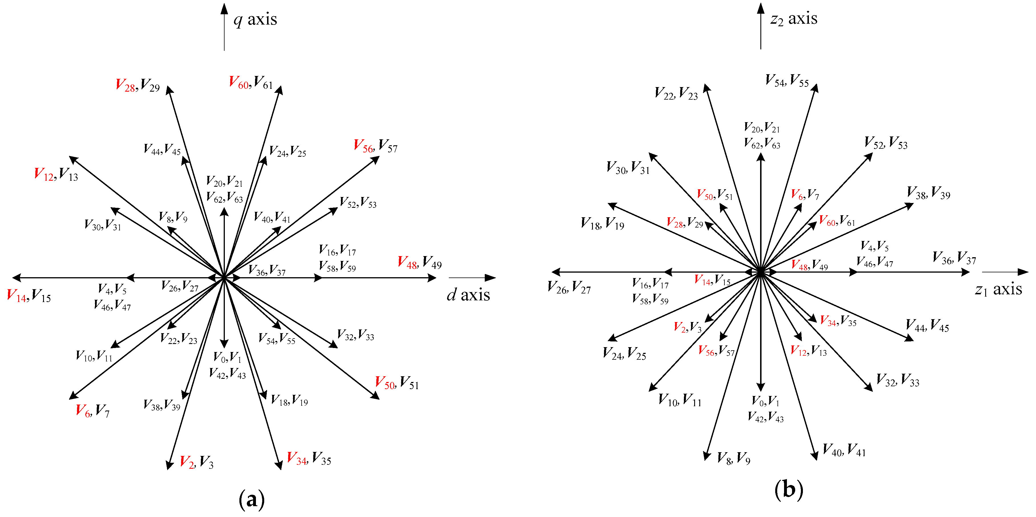
After the F-phase winding becomes open-circuited, the F-phase leg become inoperative to the motor, and the 64 switching states reduce to 25 = 32. In this case, the winding voltages uA, uC, and uE can take five values: −2Ud/3 (Ud is the DC bus voltage), Ud/3, 0, Ud/3, and 2Ud/3; the winding voltages uB and uD can take two values: −Ud/2 and Ud/2. The 32 winding voltage column matrices corresponding to 32 switching states postmultiply (6); then, 32 basic voltage vectors in the d-q plane and z1-z2 plane are obtained, as shown in Figure 7. For the comparison with the non-fault-tolerant SVPWM, in this paper, these vectors are written as V0–V63. Thus, each even number in the subscripts 0–63 and its neighboring odd number represent one basic vector. Hereafter, the even numbers are used.
To suppress the stator harmonic voltages, in this paper, by using the basic vectors, some auxiliary vectors are constructed, the magnitudes of which should be as large as possible in the d-q plane but all zero in the z1-z2 plane. Then, the reference vector Vref in the d-q plane is synthesized from these auxiliary vectors. Based on this idea, the auxiliary vectors are constructed with the following optimal model
where Vh is the h-th basic vector from 32 basic vectors; Th is the activation duration of the h-th basic vector, which is an optimal variable; is the magnitude of the synthesis result of the 32 basic vectors; is the sum of 32 activation durations; T′ is a time interval that is smaller than the switching period.
The objective function of (3) shows that a larger in the d-q plane is better to improve the dc bus voltage utilization. The constraint conditions of (3) as follows: the activation duration of each basic vector is a nonnegative value; the sum of the 32 activation durations is equal to a smaller time interval than the switching period; and in the z1-z2 plane is equal to zero in order to suppress the stator harmonic voltages.
By applying the interior point algorithm to solve (8), the following two solutions are obtained.
By applying the sequence quadratic programming algorithm to solve (8), the following four solutions are obtained.
According to (9)–(14), the following six auxiliary vectors V1′ to V6′ can be constructed.
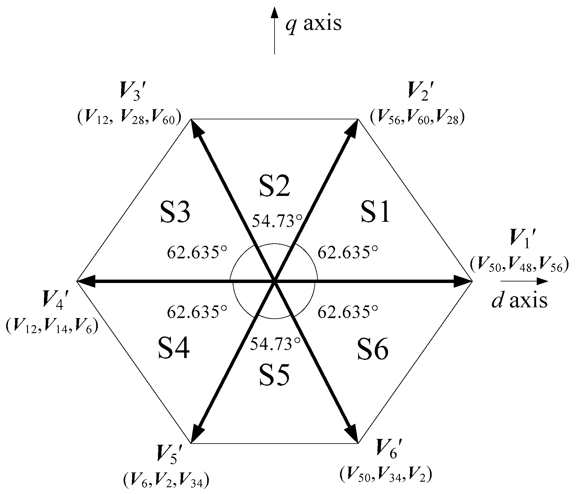
All magnitudes of the six auxiliary vectors in the z1-z2 plane are zero. The six auxiliary vectors in the d-q plane are shown in Figure 8, where the magnitudes of V1′ and V4′ are equal to Ud, and others are equal to 0.9194 Ud. By taking the auxiliary vectors as the boundary, the d-q plane can be divided into six sectors, which are labelled S1 to S6 in Figure 8. The central angles of sectors S2 and S5 are 54.73°, and others are 62.635°. Thus, the six auxiliary vectors form a nonregular hexagon.
2.4. Synthesis of Reference Vector
In each of the six sectors, the reference vector Vref is synthesized by using the auxiliary vectors at the initial side of and terminal side of the sector. In the synthesis process, in addition to the two auxiliary vectors, the null vectors in the d-q plane are required. Because the 32 basic vectors have nonzero magnitude in the d-q plane, no null vector is available in the d-q plane. It is necessary to construct some equivalent null vectors, the magnitudes of which are zero in the d-q plane but should be as small as possible in the z1-z2 plane to suppress the stator harmonic voltages. Based on this idea, the equivalent null vectors are constructed by using the following optimal model
where the meanings of the parameters except T0′ are similar to those in (8). T0′ is an activation duration of an equivalent null vector, which is smaller than the switching period.
By applying the interior point algorithm and sequence quadratic programming algorithm to solve (16), a unique solution is obtained as follows.
According to (17), an equivalent null vector V0′ can be constructed.
In sector S1, reference vector Vref is synthesized with V1′, V2′, and V0′. Let T1′, T2′, and T0′ be the activation durations of V1′, V2′, and V0′ during switching period Tc, respectively. Then, the following volt-second balancing equation is obtained.
Solving (19), we have
where Vref is the magnitude of the reference vector, θ is the angle between the reference vector and the auxiliary vector at the terminal side of the sector.
By combining (20) with (9), (11), (17), we obtain the activation durations of the six basic vectors V50, V48, V56, V60, V28, and V14 during the switching period. The synthesis in other sectors is similar to that in sector S1, and the specific process is no longer described.
The trajectory of the reference vector is circular in the nonregular hexagon, so the trajectory of the stator flux is also circular, which can make the torque smooth.
2.5. Sequence of Basic Vectors
The above analysis shows that there are six basic vectors, which are activated during each switching period in each sector. The number of activation sequences of six basic vectors is 6! = 720. According to different performance requirements, one can select the required sequence from the 720 sequences. In this paper, to reduce the switching loss as much as possible, the sequences with the fewest switching operations are selected. To find the desired sequences, if the number of switching operations of the 720 sequences is individually examined, the workload would be too large. Thus, we propose a sorting approach according to the principle of optimality.
Step 1: Construct set G = {Gj|j = 1, 2, 3, …, 6} with 6 elements, i.e., the 6 basic vectors that are activated during a switching period.
Step 2: Randomly select an element from set G as the starting vector. Remove the starting vector from set G, which now has 5 elements.
Step 3: Arrange the starting vector with each element in set G to obtain 5 permutations, from which l permutations with the fewest switching operations are selected. Remove l vectors from set G, which now has (5 − l) elements.
Step 4: Arrange these l permutations with each element in set G to obtain l·(5 − l) permutations, from which w permutations with the fewest switching operations are selected. Remove w vectors from set G, which now has (5 − l − w) elements.
Step 5: Repeat Step 4 until set G is empty and the sorting ends.
The workload of the proposed sorting approach is small. The required sequence can be quickly obtained by programming.
To make the SVPWM waveform symmetrical, the positive sequence is used in the first half period of each switching period, while the reverse sequence is used in the latter half period. For example, in sector S1, the positive sequence is V50–V48–V56–V60–V28–V14, while the reverse sequence is V14–V28–V60–V56–V48–V50, and 12 switching operations occur during one switching period. The situation in other sectors is similar to that in sector S1, as shown in Table 1.
3. Simulations and Experiments
To verify the correctness and effectiveness of the proposed method (i.e., the fault-tolerant SVPWM), we perform simulations and experiments using the non-fault-tolerant SVPWM and fault-tolerant SVPWM and compare their results.
3.1. Simulation Results
The simulation model of the system, which is composed of a six-phase induction motor and a two-level inverter, is created in MATLAB/Simulink (R2013b, The MathWorks, Inc., Natick, MA, USA) The simulation parameters are shown in Table 2.
The simulation process is as follows: the motor is started under no-load at 0 s; a 30 N·m load torque is applied at 0.4 s; the F-phase winding becomes open-circuit at 0.6 s; the simulation stops at 0.9 s. Two simulations are performed: in simulation 1, the non-fault-tolerant SVPWM is used before and after the opening; in simulation 2, the non-fault-tolerant SVPWM is used before the opening, and the fault-tolerant SVPWM is used after the opening. The simulation results are shown in Figure 9, Figure 10, Figure 11 and Figure 12, where the two simulations have identical waveforms before the opening but different waveforms after the opening.
Figure 9 shows the stator winding voltages in simulations 1 and 2. For the convenience of analysis, a low-pass filtering is made. The comparison between Figure 9a,b shows that before the opening the waveforms of the three-phase ACE-winding group are sine waves with amplitude 121 V, frequency 50 Hz, and phase difference 120°, which are phase-advanced by 30° with respect to the waveforms of the three-phase BDF-winding group. Therefore, the six voltages are balanced before the opening but unbalanced after the opening. After the opening, uF is no longer displayed because uF is uncertain and uncontrollable.
Figure 9c,d show the ACE-winding voltages by low-pass filtering in simulations 1 and 2, respectively. After opening, the waveforms in simulation 1 are unaffected, whereas the waveforms in simulation 2 change. Although the frequency and phase difference of the waveforms in simulation 2 are unchanged, the amplitudes increase. Figure 9e,f show the BDF-winding voltages by low-pass filtering in simulations 1 and 2, respectively. After opening, the frequency and phase difference of the waveforms in the two simulations are unchanged, but both amplitudes change. In simulation 1, the amplitude of uB decreases, while that of uD increases. In simulation 2, the amplitudes of uB and uD increase. Figure 9 indicates that after opening, the frequency and phase difference of the remaining healthy phase winding voltages in the two simulations are unchanged, but both amplitudes change, and simulation 2 has larger amplitudes than simulation 1.
Figure 10 shows the decoupling plane voltages by low-pass filtering in the two simulations. Figure 10a,b show the d-q axis voltages in simulations 1 and 2, respectively. Before opening, the waveforms are sine waves with amplitude 210 V, frequency 50 Hz and phase difference 90°, which illustrates that the two-phase equivalent system is symmetric. After opening, in simulation 1, the ud waveform is unchanged, but the amplitude of uq decreases; in simulation 2, the waveforms of ud and uq are unchanged. Thus, the two-phase equivalent system is asymmetric in simulation 1 but symmetric in simulation 2.
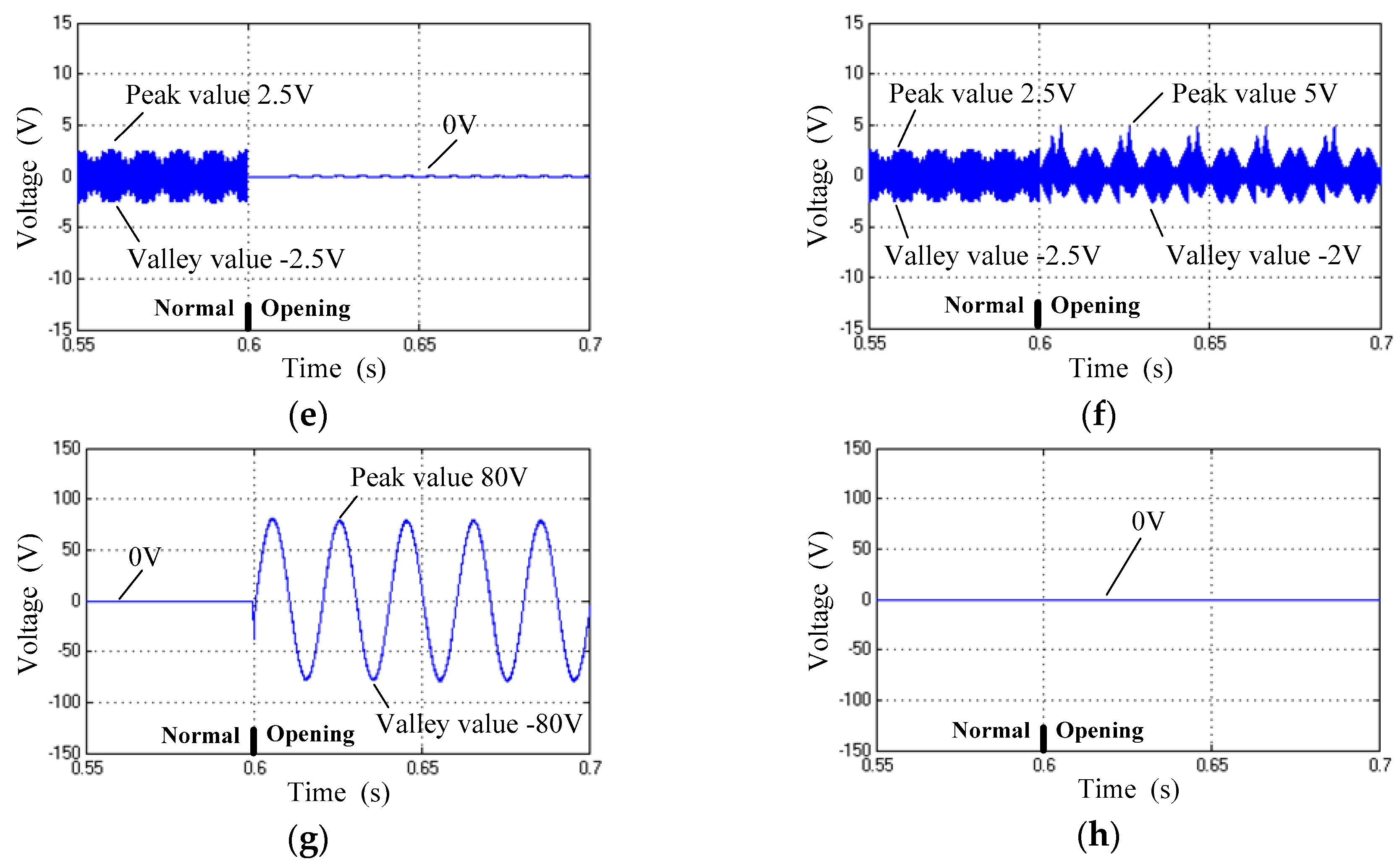
Figure 10c–h show the z1 axis, z2 axis and z3 axis voltages. For the z1 axis voltage, before the opening, the peak value is 2.5 V and the valley value is −2.5 V, so the peak-to-valley value is 5 V. After the opening, the voltages in simulation 1 remain unchanged, while in simulation 2, the peak value is 2 V and the valley value is −4 V, so the peak-to-valley value is 6 V. For the z2 axis voltage, before opening the peak-to-valley value is 5 V. After the opening, the peak-to-valley value in simulation 1 becomes zero, while in simulation 2, the peak value is 5 V and the valley value is −2 V, so the peak-to-valley value is 7 V. For the z3 axis voltage, before opening, the value is 0V. After opening, the voltage in simulation 1 becomes a sine wave with maximum amplitude of 80 V and frequency 50 Hz, while the value in simulation 2 remains 0 V. Figure 10c–h indicate that after opening, simulation 2 has lower harmonic voltages than simulation 1.
Figure 11 shows the stator winding currents in the two simulations. The comparison of Figure 11a,b shows that before opening, the waveforms of the three-phase ACE-winding group are sine waves with amplitude 10 A, frequency 50 Hz, and phase difference 120°, which are phase-advanced by 30° with respect to the waveforms of the three-phase BDF-winding group. Therefore, the six currents are balanced before the opening but unbalanced after opening. After opening, iF is 0 A.
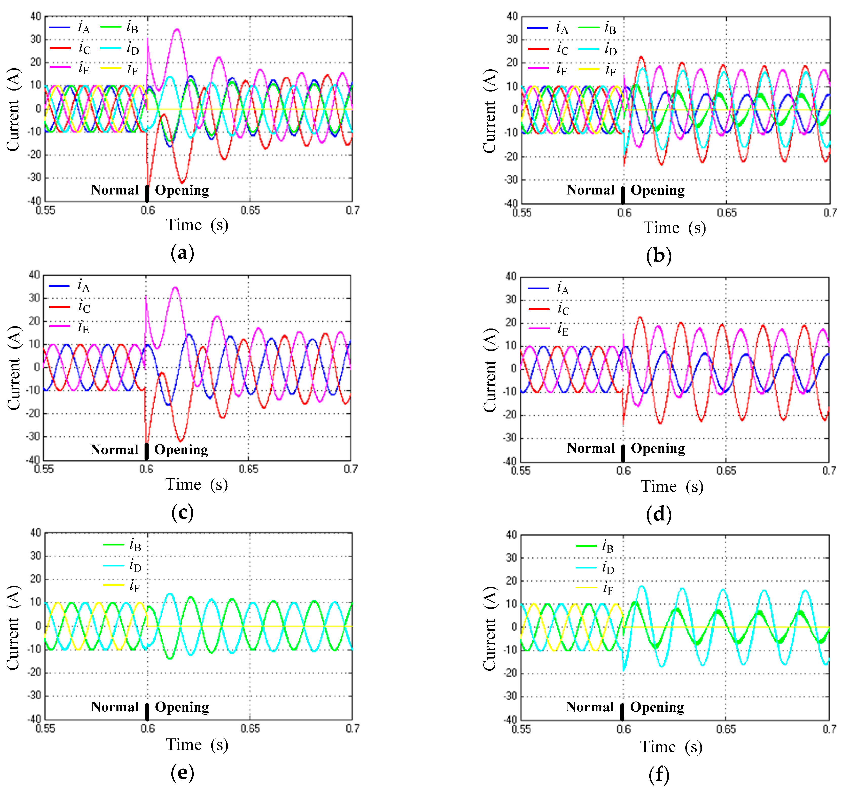
Figure 11c,d show the ACE-winding currents in simulations 1 and 2, respectively. After opening, the steady-state amplitudes in simulation 1 are 12 A, 15 A and 15 A, and the phase difference is 120°. Those in simulation 2 are 8 A, 20.35 A and 13.75 A, the DCoffset values are −1.5 A, −1.5 A and 3.25 A, and the phase difference is no longer 120°. Figure 11e,f show the BDF-winding currents in simulations 1 and 2, respectively. After opening, in the steady state, iB = −iD in simulation 1, and the amplitude is 11.2 A, while iB ≠ iD in simulation 2, the iB amplitude is 6.2 A, and the iD amplitude is 16 A. Figure 8 shows the following characteristic of the current waveforms in simulation 1: the frequency does not change, the phase difference changes, and the amplitudes change, but there is no DCbias. In comparison, in simulation 2, the frequency does not change, the phase difference change, the amplitudes change and there is a DCbias. The characteristic of the waveforms in simulation 2 maintain the circular trajectory of the stator flux.
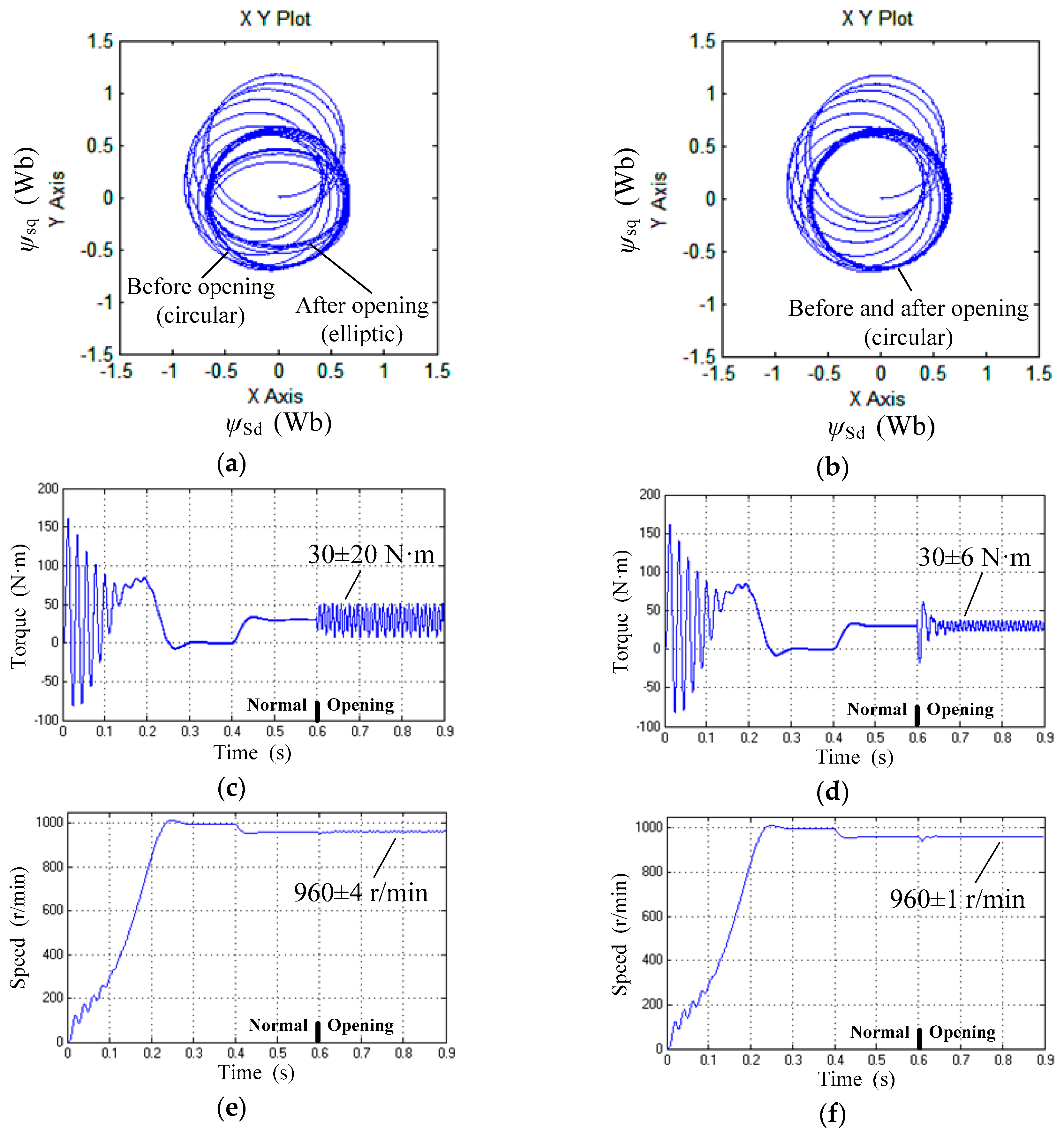
Figure 12a,b show the stator flux trajectories in simulations 1 and 2, respectively. Before opening, both steady-state flux trajectories are circular, and the amplitudes are 0.65 Wb. After opening, the steady-state flux trajectory in simulation 1 becomes elliptic, the maximum amplitude is 0.65 Wb, and the minimum amplitude is 0.4 Wb. In comparison, the flux trajectory in simulation 2 remains unchanged.
Figure 12c,d show the electromagnetic torques in simulations 1 and 2, respectively. The steady-state torques after the opening are 30 ± 20 N·m and 30 ± 6 N·m, i.e., the torque pulsation range in simulation 2 is 30% that in simulation 1.
Figure 12e,f show the rotor speeds in simulations 1 and 2, respectively. In the steady state, the no-load speeds are 1000 r/min and the load speeds are 960 r/min. There is speed drop because this is an open loop simulation, which can be reduced or even eliminated by speed feedback control. The steady-state speeds after the opening are 960 ± 4 r/min and 960 ± 1 r/min, showing that the speed pulsation range in simulation 2 is 25% that in simulation 1.
The simulation results show that under the F-Phase open-circuit fault condition and under the excitation of two types of voltage waves of the non-fault-tolerant SVPWM and fault-tolerant SVPWM, the two-phase equivalent systems are asymmetric and symmetric, and the stator flux trajectories are elliptic and circular, respectively. The latter has smaller harmonic voltages than the former; the torque pulsation range and speed pulsation range of the latter are 30% and 25% that of the former, respectively.
3.2. Experimental Results
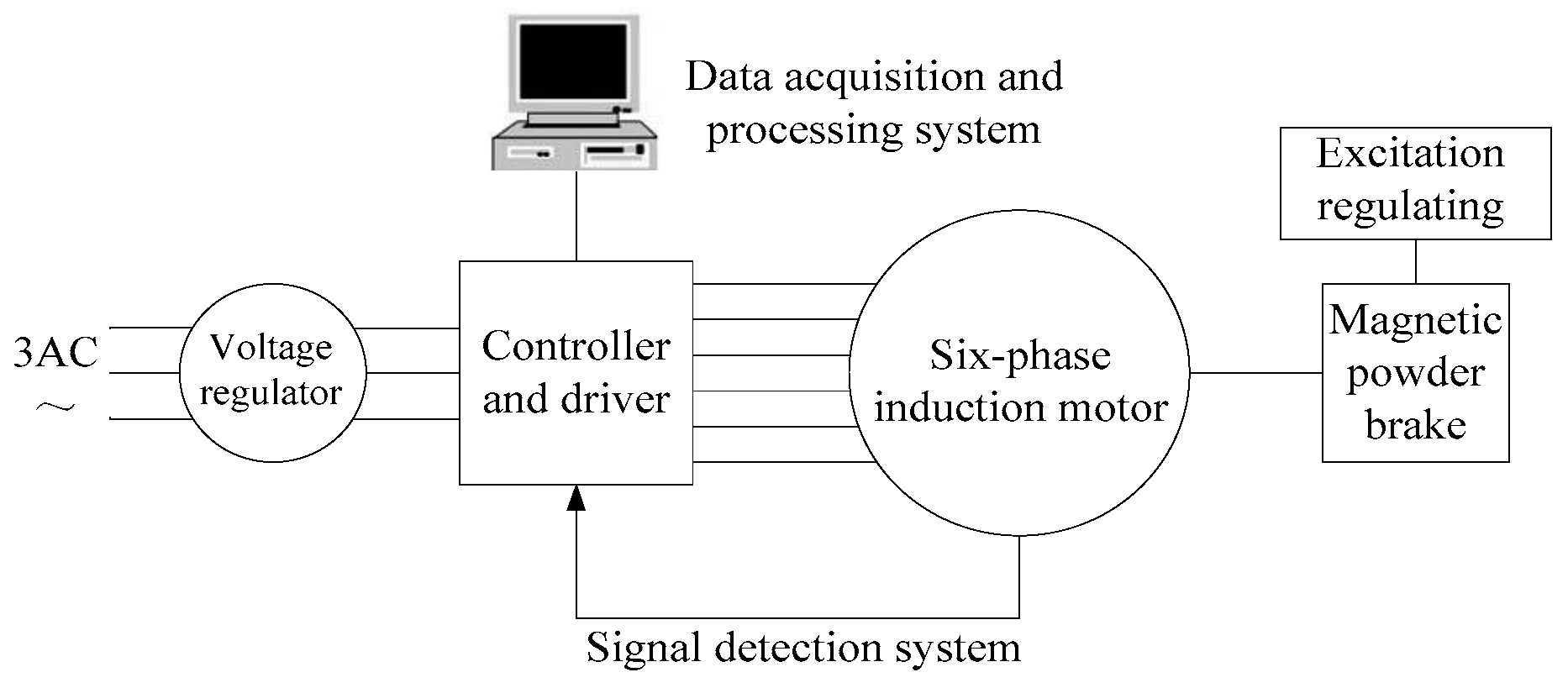
The experimental platform consists of a voltage regulator, a controller and driver, a six-phase induction motor, a magnetic powder brake, a signal (voltages and currents, torques and speeds) detection system, and a data acquisition and processing system, as shown in Figure 13.
The controller and driver (Changsha Point Rain Information Technology Ltd., Changsha, China) consists of a three-phase uncontrolled rectifier (Changsha Point Rain Information Technology Ltd., Changsha, China), a voltage stabilizing circuit (Changsha Point Rain Information Technology Ltd., Changsha, China), a six-phase inverter (Changsha Point Rain Information Technology Ltd., Changsha, China) and a digital signal processing (DSP) board (Changsha Point Rain Information Technology Ltd., Changsha, China). Three-phase 380 V/50 HZ AC is converted to 260 V DC by the voltage regulator, the three-phase uncontrollable rectifier and voltage stabilizing circuit. The six-phase inverter consists of two three-phase intelligent power modules (IPMs), and the DSP chip is TMS320F28335. The SVPWM signals from the DSP board are sent to the IPMs after an isolation circuit to drive the six-phase inverter. The magnetic powder brake is a loading device, which adjusts the load torque by regulating the excitation current. The signal detection system detects the DC bus voltage, the stator phase currents and the rotor speed, which are sent to the DSP board. The DC bus voltage is measured by a Hall voltage sensor, the stator phase currents are measured by six Hall current sensors, and the rotor speed is measured by a photoelectric encoder. The DSP board calculates the stator phase voltages by the DC bus voltage, and calculates the electromagnetic torque by the phase voltages and currents. The data acquisition and processing system uses a personal computer, which communicates with the DSP board by the bus to read the detection and calculation results. The experimental device is shown in Figure 14.
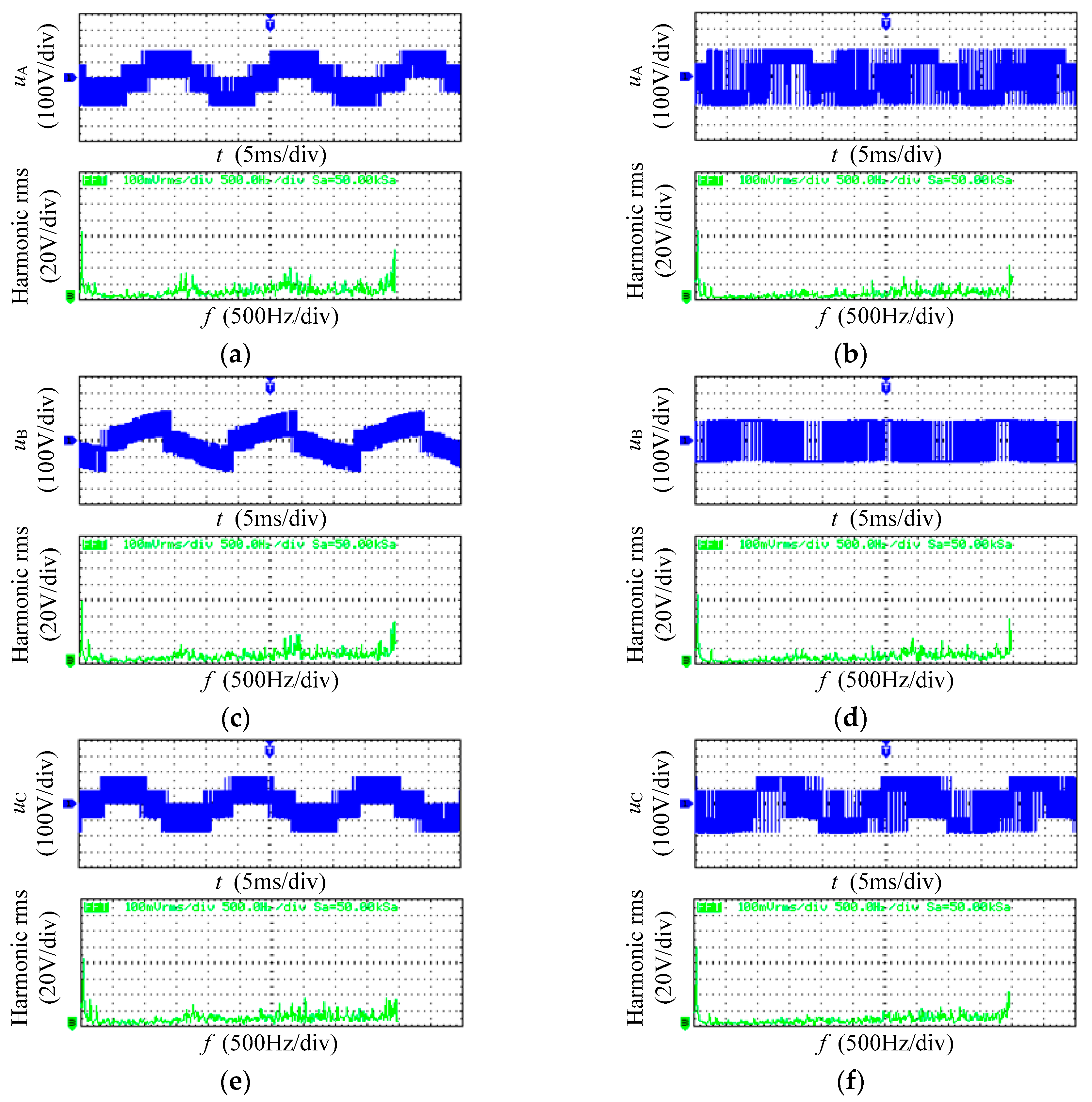
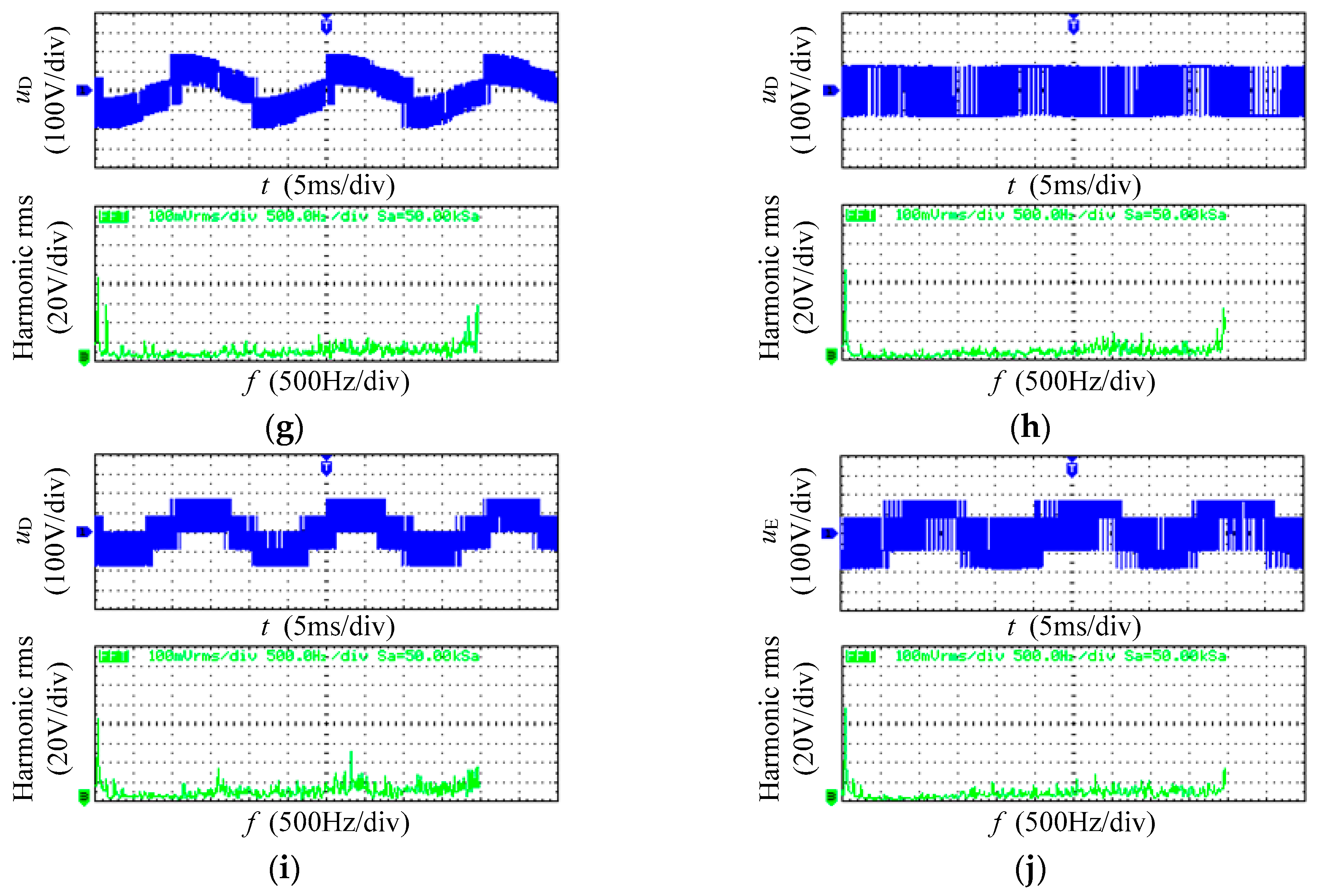
The experiment parameters are identical to the simulation parameters, as shown in Table 2.The experimental process is similar to the simulation process: the motor is started under no-load at 0 s; a 30 N·m load torque is applied at 40 s; the F-phase winding becomes open-circuit at 60 s; the experiment stops at 90 s. Two experiments are performed: in experiment 1, the non-fault-tolerant SVPWM is used before and after the opening; in experiment 2, the non-fault-tolerant SVPWM is used before opening, and the fault-tolerant SVPWM is used after opening. The experimental results are shown in Figure 15, Figure 16 and Figure 17. A fast Fourier transform (FFT) analysis of the steady-state voltages of the remaining healthy stator phase winding is performed in the data acquisition and processing system and the related results are shown in Table 3.
Figure 15 shows the waveforms of the steady-state voltages of the remaining healthy phase windings and their FFT analysis after opening in experiments 1 and 2. These figures show that the root-mean-square (rms for short in Figure 15) values of the fundamental waves in experiment 2 are larger than those in experiment 1, which is also observed in Table 3. In Table 3, the amplitudes of the fundamental waves in experiment 2 are larger than those in experiment 1. In addition, Table 3 shows experiment 2 has a smaller total harmonic distortion (THD) rate than experiment 1, which indicates that experiment 2 has smaller harmonic voltages than experiment 1.
Figure 16 shows the waveforms of the steady-state currents of iA and iC, iB, and iD after opening in experiments 1 and 2. The difference in current amplitudes of the four windings is not large in experiment 1, but large in experiment 2. The waveform characteristic of the latter can facilitate the maintenance of the circular trajectory of the stator flux.
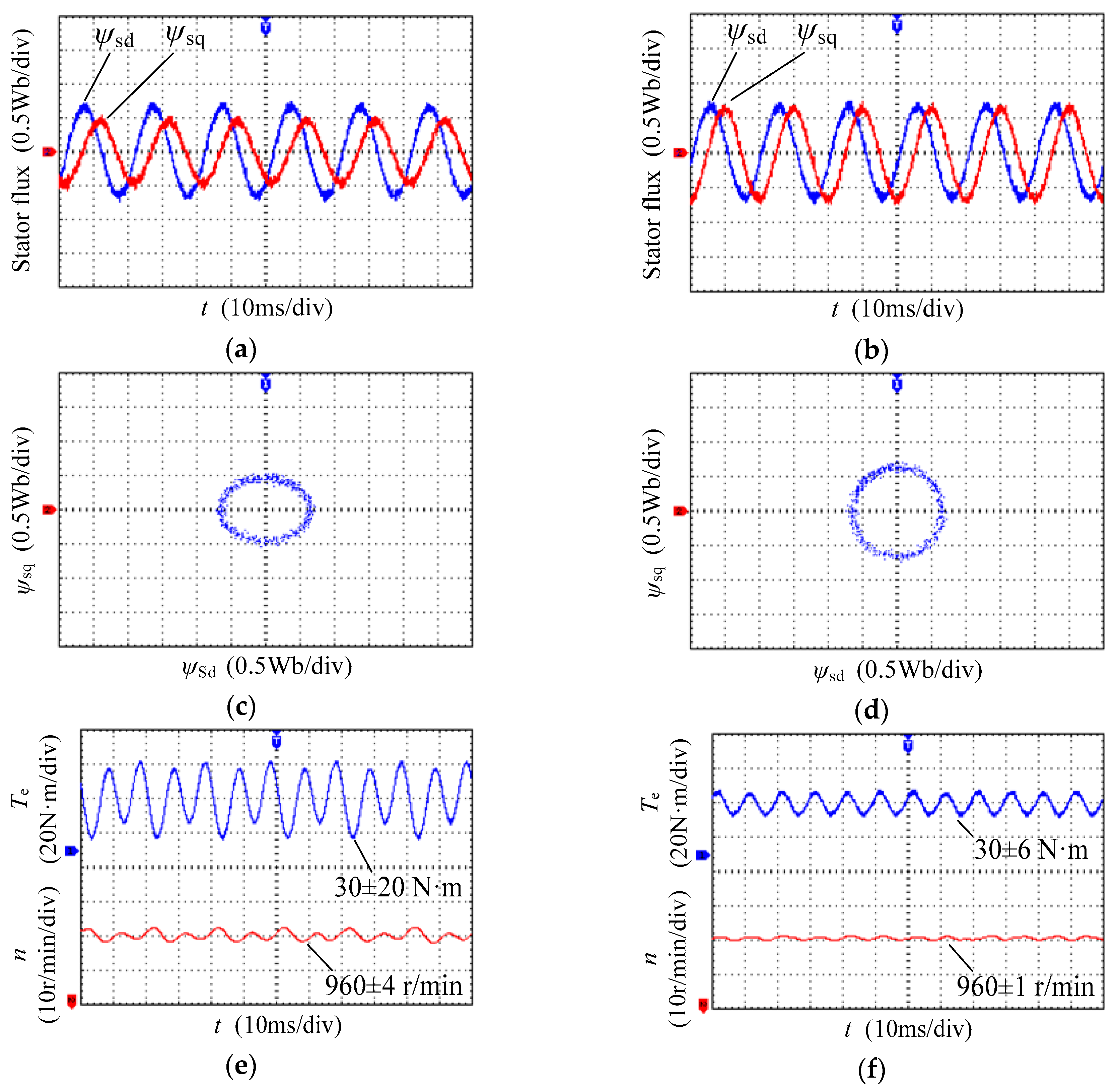
Figure 17a,b show the d-q axis steady-state stator fluxes after opening in experiments 1 and 2, respectively. These waveforms show that both phase differences between d-axis flux ψsd and q-axis flux ψsd are 90°. In experiment 1, the amplitude of ψsq is smaller than that of ψsd, whereas in experiment 2, ψsq and ψsd have equal amplitudes. Thus, the two-phase equivalent system of non-fault-tolerant SVPWM is asymmetric, while that of fault-tolerant SVPWM is symmetric.
Figure 17c,d show the steady-state stator flux trajectories after opening in experiments 1 and 2, respectively. The trajectory in experiment 1 is elliptic, while the trajectory in experiment 2 is circular.
Figure 17e,f show the steady-state torques and speeds after the opening in experiments 1 and 2, respectively. The pulsation frequency of the torque and speed in experiment 1 is identical to that in experiment 2, which is three times the power frequency 50 Hz. The range of the torque pulsation in experiment 1 is 30 ± 20 N·m, and the pulsation amplitude strongly fluctuates. In comparison, that in experiment 2 is only 30 ± 6 N·m, and the pulsation amplitude is relatively constant. Similarly, the range of the speed pulsation in experiment 1 is 960 ± 4 r/min, and the pulsation amplitude fluctuates, whereas that in experiment 2 is only 960 ± 1 r/min, and the pulsation amplitude is relatively constant. These experimental results show that the fault-tolerant SVPWM can effectively improve the phase-deficient operation performance of the system.
4. Conclusions
In the system of the six-phase motor and two-level inverter, when the stator one-phase open-circuit fault occurs, the star point of the open-circuit winding group is connected to the centre point of the inverter dc voltage; then, the SVPWM technology can be used. It is unnecessary to connect the star point of the healthy winding group to the centre point of the inverter dc voltage.
When the stator one-phase open-circuit fault occurs, the five-dimensional orthogonal matrix can be constructed. The matrix can follow the equivalent principle of equal magnetic motive force and equal power before and after transformation, while satisfying the current constraint condition of the remaining healthy phase windings. Thus, the order of the original differential equation of the motor can be reduced using the matrix.
By using the matrix, the 32 winding voltage column matrices that correspond to the 32 switching states are mapped to the electromechanical energy conversion plane (the d-q plane) and non-electromechanical energy conversion plane (the z1-z2 plane), and 32 basic vectors are obtained. By using the optimal model, six auxiliary vectors and one equivalent null vector can be constructed, the magnitudes of which are all zero in the z1-z2 plane. By using the auxiliary vectors and equivalent null vector, the reference vector is synthesized, the zero magnitude of which in the z1-z2 plane can suppress the harmonic voltages, and the circular trajectory of which in the d-q plane can make the torque smooth.
The simulation and experimental results show that the proposed method has smaller harmonic voltages than the classical method; the stator flux trajectory of the proposed method is circular while that of the classical method is elliptic. The torque pulsation range and speed pulsation range of the proposed method are 30% and 25% of those of the classical method, respectively. Therefore, the phase-deficient operation performance of the system is improved. The proposed method can be further extended to arbitrary-phases open-circuit fault of multiphase machines.
Author Contributions
All the contributions in this paper are equally shared among the authors.
Funding
This research was funded by National Natural Science Foundation of China under Project 51737004 and National Key Research and Development Program of China under Project 2016YFF0203400.
Conflicts of Interest
The authors declare no conflicts of interest.
References
- Barrero, F.; Duran, M.J. Recent advances in the design, modeling, and control of multiphase machines—Part I. IEEE Trans. Ind. Electron. 2016, 63, 449–458. [Google Scholar] [CrossRef]
- Barrero, F.; Duran, M.J. Recent advances in the design, modeling, and control of multiphase machines—Part II. IEEE Trans. Ind. Electron. 2016, 63, 459–468. [Google Scholar] [CrossRef]
- Che, H.S.; Levi, E.; Jones, M.; Duran, M.J.; Hew, W.; Rahim, N.A. Operation of a six-phase induction machine using series-connected machine-side converters. IEEE Trans. Ind. Electron. 2014, 61, 164–176. [Google Scholar] [CrossRef]
- Tir, Z.; Malik, O.P.; Eltamaly, A.M. Fuzzy logic based speed control of indirect field oriented controlled Double Star Induction Motors connected in parallel to a single six-phase inverter supply. Electr. Power Syst. Res. 2016, 134, 126–133. [Google Scholar] [CrossRef]
- Levi, E. Advances in converter control and innovative exploitation of additional degrees of freedom for multiphase machines. IEEE Trans. Ind. Electron. 2016, 63, 433–448. [Google Scholar] [CrossRef]
- Xu, P.; Feng, J.H.; Guo, S.Y.; Feng, S.; Chu, W.; Ren, Y.; Zhu, Z.Q. Analysis of dual three-phase permanent-magnet synchronous machines with different angle displacements. IEEE Trans. Ind. Electron. 2018, 65, 1941–1954. [Google Scholar] [CrossRef]
- Zheng, P.; Wu, F.; Lei, Y.; Sui, Y.; Yu, B. Investigation of a novel 24-slot/14-pole six-phase fault-tolerant modular permanent-magnet in-wheel motor for electric vehicles. Energies 2013, 6, 164–176. [Google Scholar] [CrossRef]
- Zhao, Y.; Lipo, T.A. Space vector PWM control of dual three-phase induction machine using vector space decomposition. IEEE Trans. Ind. Appl. 1995, 31, 1100–1108. [Google Scholar] [CrossRef]
- Alberti, L.; Bianchi, N. Experimental tests of dual three-phase induction motor under faulty operating condition. IEEE Trans. Ind. Electron. 2012, 59, 2041–2048. [Google Scholar] [CrossRef]
- Duran, M.J.; Gonzalez-Prieto, I.; Rios-Garcia, M.; Barrero, F. A simple, fast, and robust open-phase fault detection technique for six-phase induction motor drives. IEEE Trans. Power Electron. 2018, 33, 547–557. [Google Scholar] [CrossRef]
- Che, H.S.; Duran, M.J.; Levi, E.; Jones, M.; Hew, W.; Rahim, N.A. Postfault operation of an asymmetrical six-phase induction machine with single and two isolated neutral points. IEEE Trans. Power Electron. 2014, 29, 5406–5416. [Google Scholar] [CrossRef]
- Munim, W.N.W.A.; Duran, M.J.; Che, H.S.; Bermudez, M.; Gonzalez-Prieto, I.; Rahim, N.A. A unified analysis of the fault tolerance capability in six-phase induction motor drives. IEEE Trans. Power Electron. 2017, 32, 7824–7836. [Google Scholar] [CrossRef]
- Kong, W.; Kang, M.; Li, D.; Qu, R.; Jiang, D.; Gan, C. Investigation of spatial harmonic magnetic field coupling effect on torque ripple for multiphase induction motor under open fault condition. IEEE Trans. Power Electron. 2018, 33, 6060–6071. [Google Scholar] [CrossRef]
- Zhao, Y.; Lipo, T.A. Modeling and control of a multi-phase induction machine with structural unbalance. IEEE Trans. Energy Convers. 1996, 11, 570–577. [Google Scholar] [CrossRef]
- Geng, Y.W.; Bao, Y.; Wang, H.; Ma, H. Direct torque and fault tolerant control for six-phase induction motor. Proc. CSEE 2016, 36, 5947–5956. [Google Scholar]
- Pantea, A.; Yazidi, A.; Betin, F.; Taherzadeh, M.; Carrière, S.; Henao, H.; Capolino, G. Six-phase induction machine model for electrical fault simulation using the circuit-oriented method. IEEE Trans. Ind. Electron. 2016, 63, 494–503. [Google Scholar] [CrossRef]
- Zhou, Y.; Lin, X.; Cheng, M. A fault-tolerant direct torque control for six-phase permanent magnet synchronous motor with arbitrary two opened phases based on modified variables. IEEE Trans. Energy Convers. 2016, 31, 549–556. [Google Scholar] [CrossRef]
- Tani, A.; Mengoni, M.; Zarri, L.; Serra, G.; Casadei, D. Control of multiphase induction motors with an odd number of phases under open-circuit phase faults. IEEE Trans. Power Electron. 2012, 27, 565–577. [Google Scholar] [CrossRef]
- Hu, Y.; Zhu, Z.Q.; Liu, K. Current control for dual three-phase PM synchronous motors accounting for current unbalance and harmonics. IEEE J. Emerg. Sel. Top. Power Electron. 2016, 2, 272–284. [Google Scholar]
- Baneira, F.; Doval-Gandoy, J.; Yepes, A.G.; López, O.; Perez-Estevez, D. Control strategy for multiphase drives with minimum losses in the full torque operation range under single open-phase fault. IEEE Trans. Power Electron. 2017, 32, 6275–6285. [Google Scholar] [CrossRef]
Figure 1.
System composed of the converter and six-phase machine with double Y-connected windings displaced by 30°. (a) Circuit configuration under normal condition; (b) Circuit configuration under F-phase open-circuit fault condition.
Figure 1.
System composed of the converter and six-phase machine with double Y-connected windings displaced by 30°. (a) Circuit configuration under normal condition; (b) Circuit configuration under F-phase open-circuit fault condition.
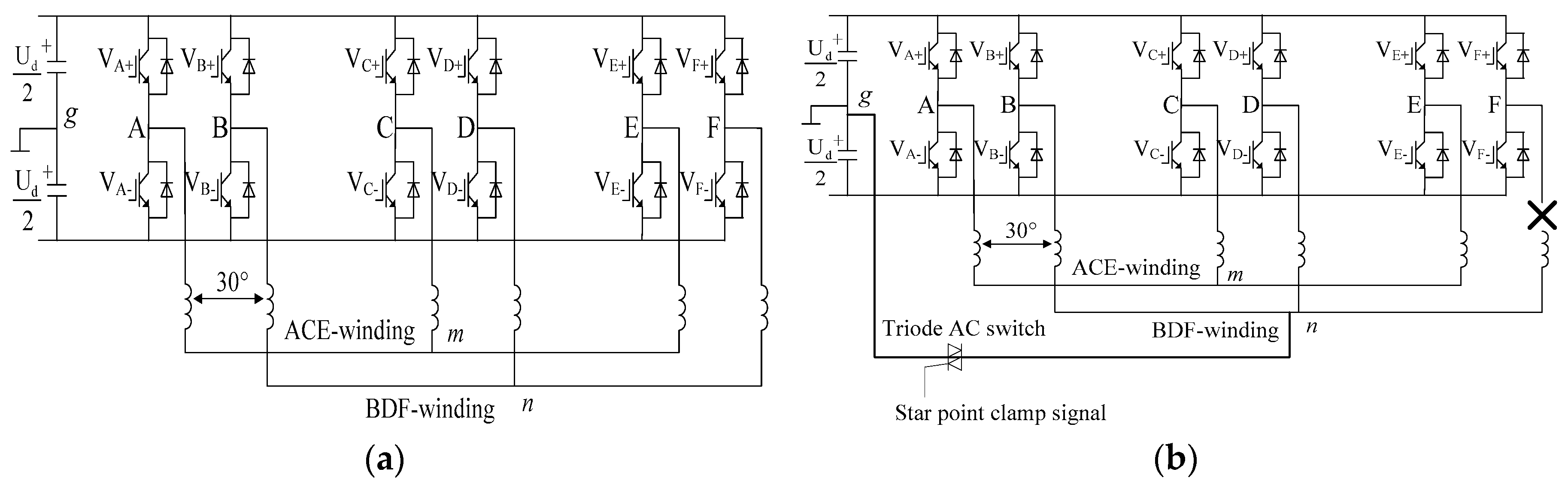
Figure 2.
Schematic diagram of SVPWM control structure.

Figure 3.
Winding terminal remarking. (a) A-phase failure; (b) B-phase failure; (c) C-phase failure; (d) D-phase failure; (e) E-phase failure; (f) F-phase failure.
Figure 3.
Winding terminal remarking. (a) A-phase failure; (b) B-phase failure; (c) C-phase failure; (d) D-phase failure; (e) E-phase failure; (f) F-phase failure.

Figure 4.
Research route of Fault-tolerant SVPWM.
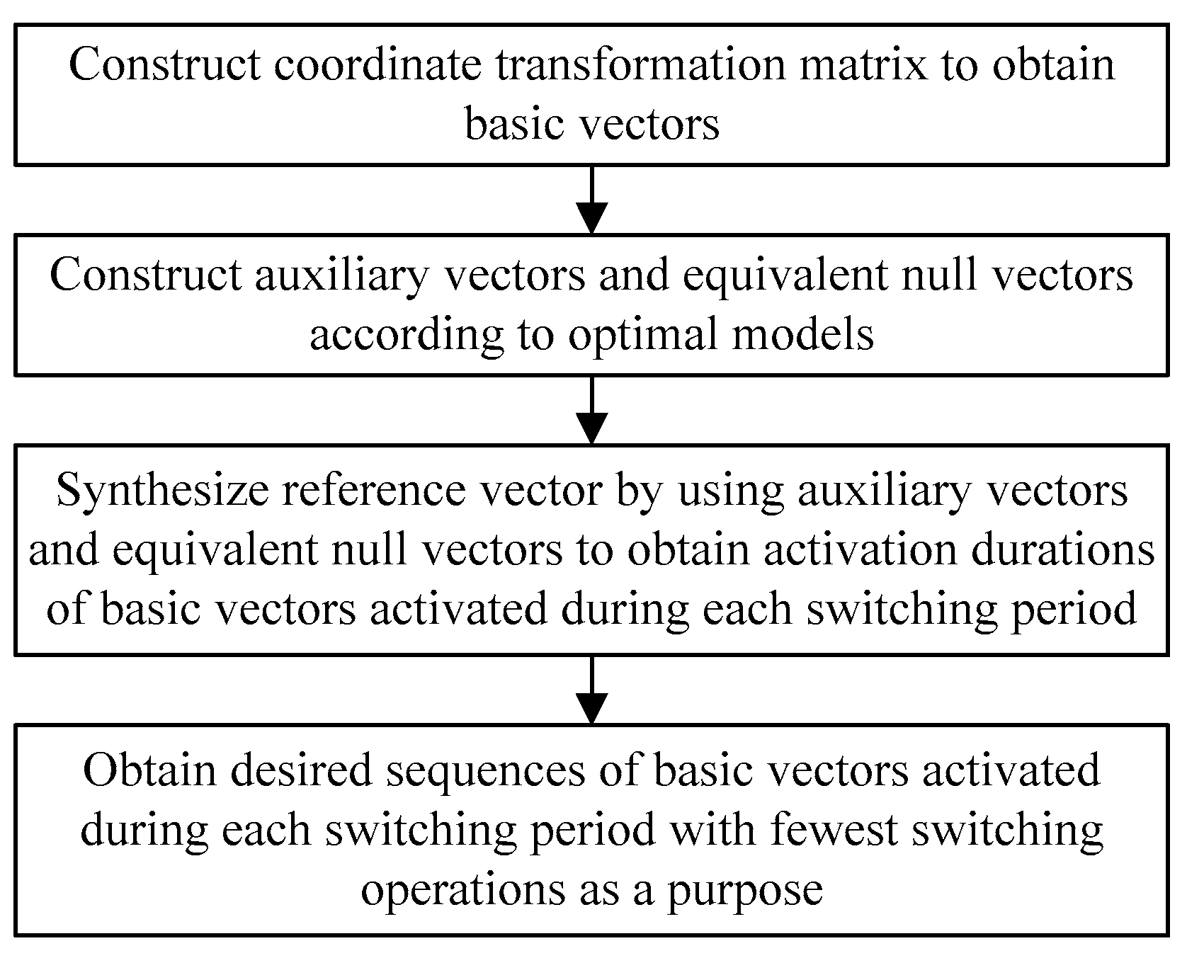
Figure 5.
Physical model of stator winding. (a) Asymmetric five-phase winding; (b) Equivalent two-phase winding.
Figure 5.
Physical model of stator winding. (a) Asymmetric five-phase winding; (b) Equivalent two-phase winding.

Figure 6.
Flow chart of constructing the coordinate transformation matrix.

Figure 7.
32 basic vectors in the d-q and z1-z2 planes. (a) 32 basic vectors in the d-q plane; (b) 32 basic vectors in the z1-z2 plane.
Figure 7.
32 basic vectors in the d-q and z1-z2 planes. (a) 32 basic vectors in the d-q plane; (b) 32 basic vectors in the z1-z2 plane.

Figure 8.
Six auxiliary vectors, six sectors, and a nonregular hexagon in the d-q plane.

Figure 9.
Stator winding voltages by low-pass filtering in simulations 1 and 2. (a) Stator winding voltages in simulation 1; (b) Stator winding voltages in simulation 2; (c) ACE-winding voltages in simulation 1; (d) ACE-winding voltages in simulation 2; (e) BDF-winding voltages in simulation 1; (f) BDF-winding voltages in simulation 2.
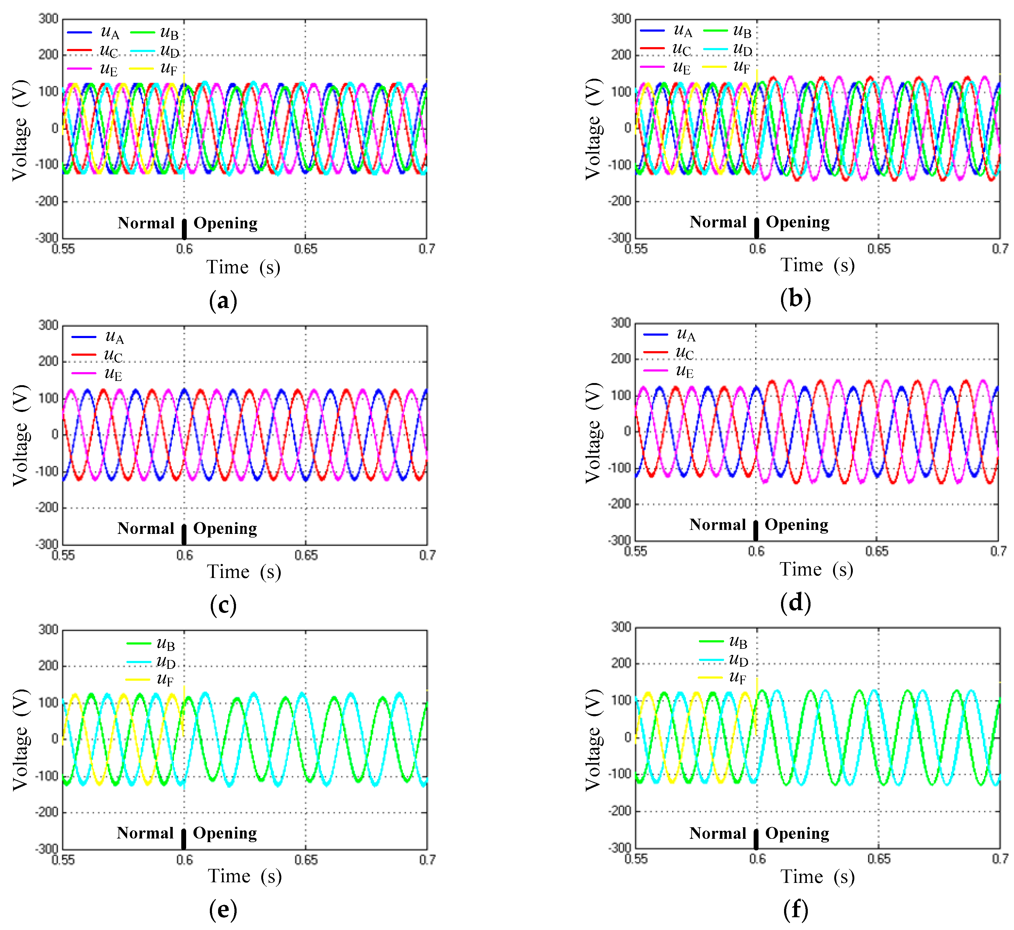
Figure 10.
Decoupling plane voltages by low-pass filtering in simulations 1 and 2. (a) d-q axis voltages in simulation 1; (b) d-q axis voltages in simulation 2; (c) z1 axis voltage in simulation 1; (d) z1 axis voltage in simulation 2; (e) z2 axis voltage in simulation 1; (f) z2 axis voltage in simulation 2; (g) z3 axis voltage in simulation 1; (h) z3 axis voltage in simulation 2.
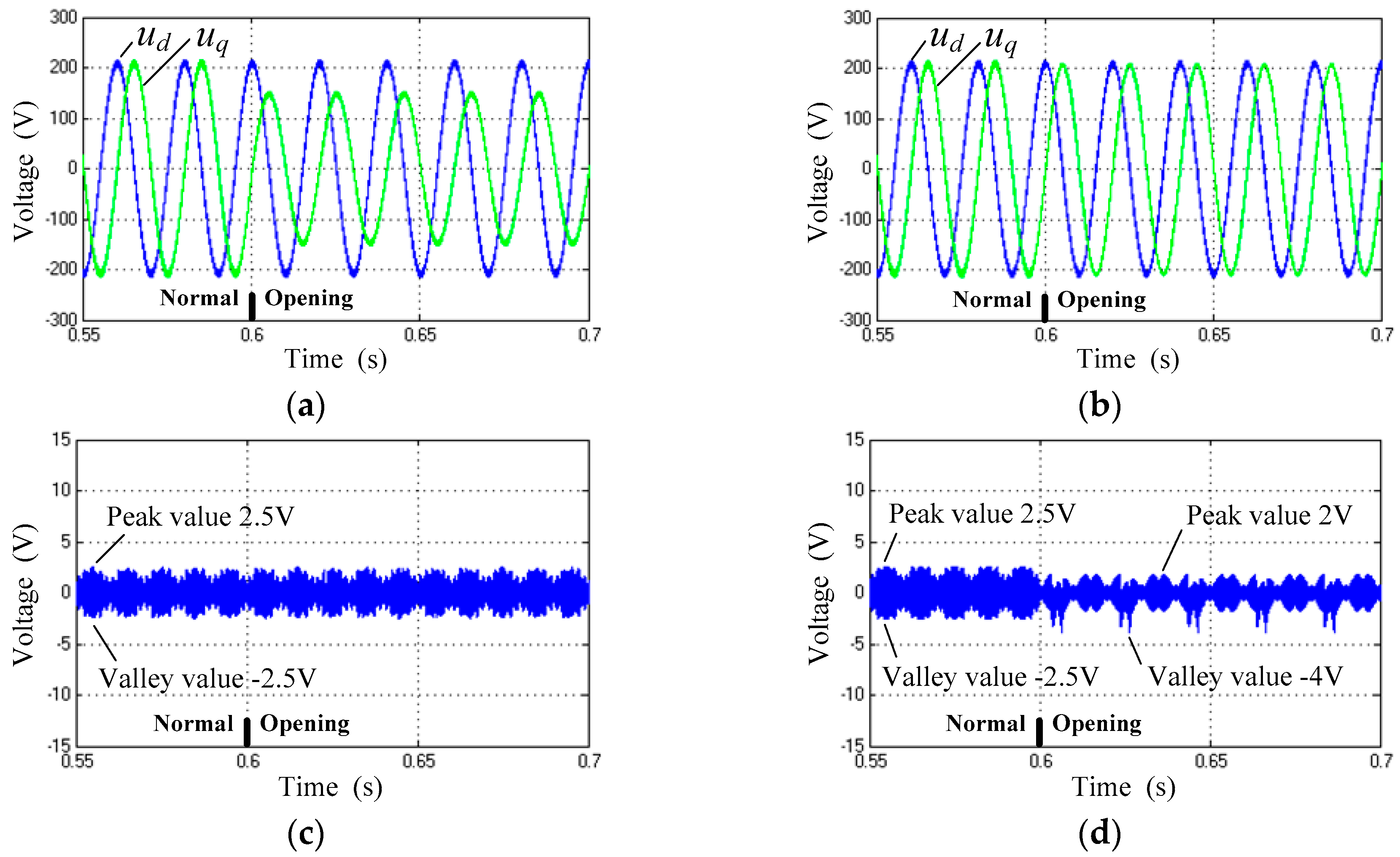

Figure 11.
Stator winding currents in simulations 1 and 2. (a) Stator winding currents in simulation 1; (b) Stator winding currents in simulation 2; (c) ACE-winding currents in simulation 1; (d) ACE-winding currents in simulation 2; (e) BDF-winding currents in simulation 1; (f) BDF-winding currents in simulation 2.

Figure 12.
Fluxes, torques, and speeds in Simulations 1 and 2. (a) Stator flux trajectory in simulation 1; (b) Stator flux trajectory in simulation 2; (c) Electromagnetic torque in simulation 1; (d) Electromagnetic torque in simulation 2; (e) Rotor speed in simulation 1; (f) Rotor speed in simulation 2.

Figure 13.
Block diagram of the experimental platform.

Figure 14.
Experimental device.
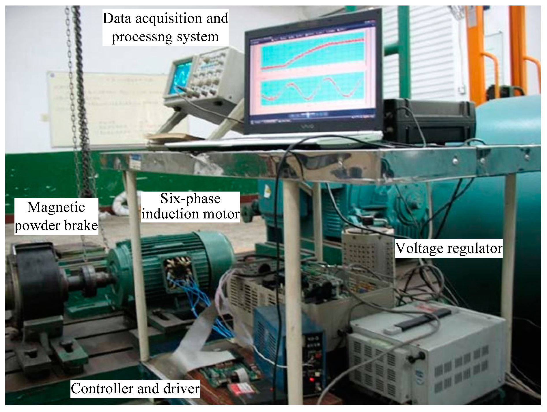
Figure 15.
Stator winding voltages and their FFT analysis in experiments 1 and 2. (a) A-phase voltage and its FFT in experiment 1; (b) A-phase voltage and its FFT in experiment 2; (c) B-phase voltage and its FFT in experiment 1; (d) B-phase voltage and its FFT in experiment 2; (e) C-phase voltage and its FFT in experiment 1; (f) C-phase voltage and its FFT in experiment 2; (g) D-phase voltage and its FFT in experiment 1; (h) D-phase voltage and its FFT in experiment 2; (i) E-phase voltage and its FFT in experiment 1; (j) E-phase voltage and its FFT in experiment 2.


Figure 16.
Stator winding currents in experiments 1 and 2. (a) AC-winding currents in experiment 1; (b) AC-winding currents in experiment 2; (c) BD-winding currents in experiment 1; (d) BD-winding currents in experiment 2.
Figure 16.
Stator winding currents in experiments 1 and 2. (a) AC-winding currents in experiment 1; (b) AC-winding currents in experiment 2; (c) BD-winding currents in experiment 1; (d) BD-winding currents in experiment 2.
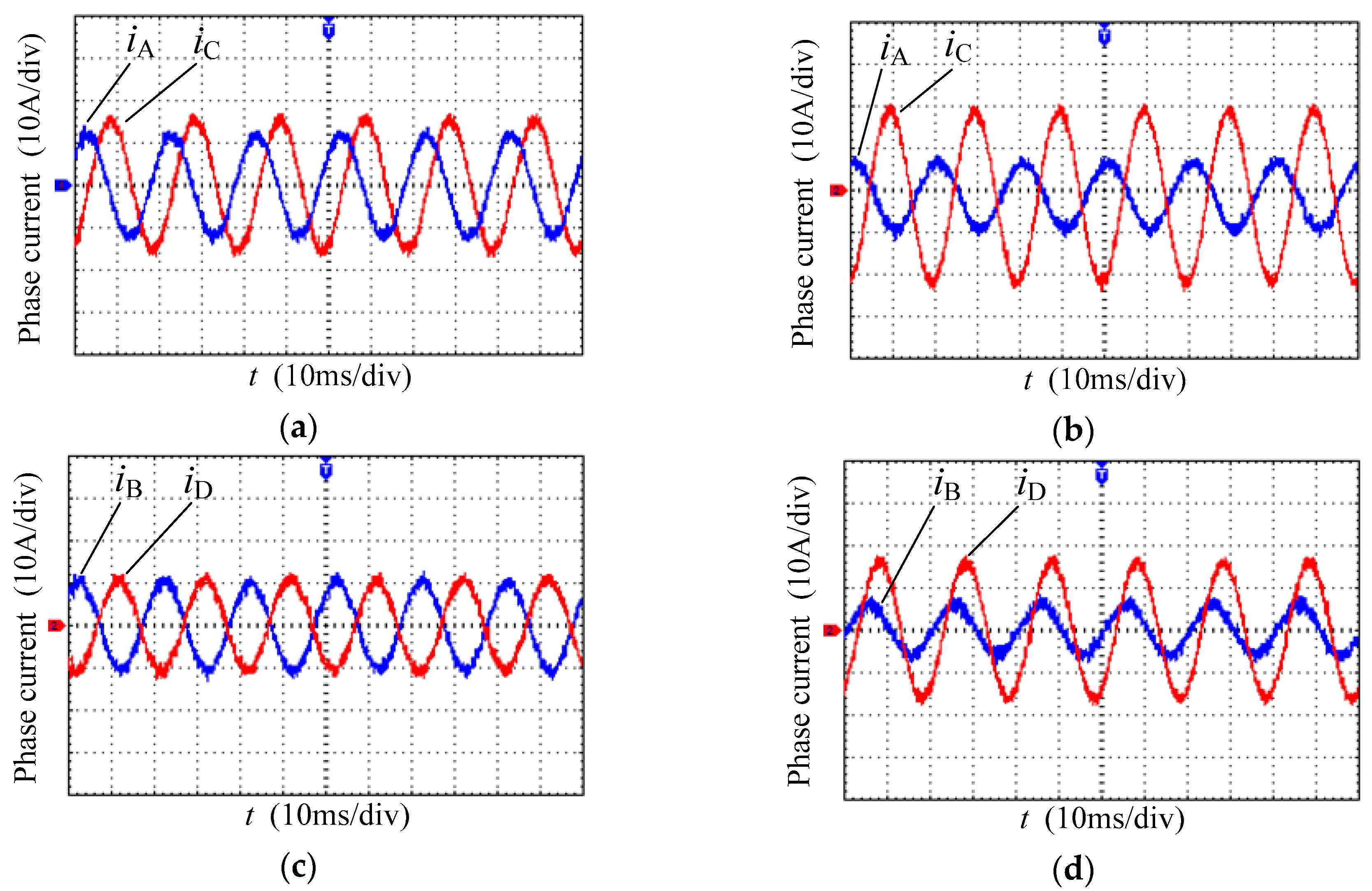
Figure 17.
Fluxes, torques, and speeds in experiments 1 and 2. (a) d-q axis stator fluxes in experiment 1; (b) d-q axis stator fluxes in experiment 2; (c) Stator flux trajectory in experiment 1; (d) Stator flux trajectory in experiment 2; (e) Torque and speed in experiment 1; (f) Torque and speed in experiment 2.

Table 1.
Sequence of basic vectors and on-off times.
| Sectors | Sequence of Basic Vectors | On-Off Times |
|---|---|---|
| S1 | V50–V48–V56–V60–V28–V14–V14–V28–V60–V56–V48–V50 | 12 |
| S2 | V48–V56–V60–V28–V12–V14–V14–V12–V28–V60–V56–V48 | 10 |
| S3 | V48–V60–V28–V12–V14–V6–V6–V14–V12–V28–V60–V48 | 12 |
| S4 | V12–V14–V6–V2–V34–V48–V48–V34–V2–V6–V14–V12 | 12 |
| S5 | V14–V6–V2–V34–V50–V48–V48–V50–V34–V2–V6–V14 | 10 |
| S6 | V14–V2–V34–V50–V48–V56–V56–V48–V50–V34–V2–V14 | 12 |
Table 2.
Simulation and experiment parameters.
| Parameters | Values | Parameters | Values |
|---|---|---|---|
| Three-phase ac voltage | 380 V/50 Hz | Moment of inertia | 0.116 kg·m2 |
| DC bus voltage | 260 V | Stator resistance | 0.22 Ω |
| Switching period | 0.0001 s | Rotor resistance | 0.47 Ω |
| Reference vector | 210 V/50 Hz | Stator inductance | 0.0395 H |
| Motor rated power | 5.5 kW | Rotor inductance | 0.0395 H |
| Motor rated voltage | 150 V/50 Hz | Mutual inductance | 0.0364 H |
| Number of pole pairs | 3 |
Table 3.
FFT analysis results of steady-state voltages of remaining healthy stator phase winding.
| Voltages | Non-Fault-Tolerant SVPWM | Fault-Tolerant SVPWM | ||
|---|---|---|---|---|
| Fundamental (50 Hz) | THD (0–5 KHz) | Fundamental (50 Hz) | THD (0–5 KHz) | |
| uA | 121.4 V | 9.97% | 125.7 V | 8.98% |
| uB | 113.4 V | 9.86% | 125.0 V | 8.73% |
| uC | 121.4 V | 9.79% | 143.3 V | 8.23% |
| uD | 124.5 V | 9.12% | 133.2 V | 8.58% |
| uE | 121.5 V | 9.82% | 138.0 V | 8.12% |
© 2018 by the authors. Licensee MDPI, Basel, Switzerland. This article is an open access article distributed under the terms and conditions of the Creative Commons Attribution (CC BY) license (http://creativecommons.org/licenses/by/4.0/).
Share and Cite
MDPI and ACS Style
Zheng, J.; Huang, S.; Rong, F.; Lye, M. Six-Phase Space Vector PWM under Stator One-Phase Open-Circuit Fault Condition. Energies 2018, 11, 1796. https://doi.org/10.3390/en11071796
AMA Style
Zheng J, Huang S, Rong F, Lye M. Six-Phase Space Vector PWM under Stator One-Phase Open-Circuit Fault Condition. Energies. 2018; 11(7):1796. https://doi.org/10.3390/en11071796
Chicago/Turabian StyleZheng, Jian, Shoudao Huang, Fei Rong, and Mingcheng Lye. 2018. "Six-Phase Space Vector PWM under Stator One-Phase Open-Circuit Fault Condition" Energies 11, no. 7: 1796. https://doi.org/10.3390/en11071796
Note that from the first issue of 2016, this journal uses article numbers instead of page numbers. See further details here.