Multi Objective Optimization in Charge Management of Micro Grid Based Multistory Carpark

1
Centre ENET at VŠB-TU Ostrava, 708 00 Ostrava, Czech Republic
2
Department of Electric Power Engineering at Faculty of Electrical Engineering and Computer Science, VŠB-TU Ostrava, 708 00 Ostrava, Czech Republic
3
Department of Computer Science at Faculty of Electrical Engineering and Computer Science, VŠB-TU Ostrava, 708 00 Ostrava, Czech Republic
*
Authors to whom correspondence should be addressed.
Energies 2018, 11(7), 1791; https://doi.org/10.3390/en11071791
Submission received: 31 May 2018
/
Revised: 26 June 2018
/
Accepted: 5 July 2018
/
Published: 8 July 2018
(This article belongs to the Special Issue Advanced Control Techniques for Power Converters)
Abstract
:Distributed power supply with the use of renewable energy sources and intelligent energy flow management has undoubtedly become one of the pressing trends in modern power engineering, which also inspired researchers from other fields to contribute to the topic. There are several kinds of micro grid platforms, each facing its own challenges and thus making the problem purely multi objective. In this paper, an evolutionary driven algorithm is applied and evaluated on a real platform represented by a private multistory carpark equipped with photovoltaic solar panels and several battery packs. The algorithm works as a core of an adaptive charge management system based on predicted conditions represented by estimated electric load and production in the future hours. The outcome of the paper is a comparison of the optimized and unoptimized charge management on three different battery setups proving that optimization may often outperform a battery setup with larger capacity in several criteria.
1. Introduction
The 20/20/20 targets defined as ’European climate and energy goals’ mean a 20% increase in the use of renewable energy sources (RES) combined with a 20% energy efficiency improvement by 2020. The European Commission sets the energy goals and benchmarks at the levels of individual buildings. A recent European Directive (2010/31/EU) targets a high deployment of RES and energy efficiency in the built environment by requiring that all new buildings need to be nearly zero energy buildings (nZEB) by 2020 [1]. Emerging trends of the electric vehicle (EV) deployments, on the other hand, call for innovations in these areas to achieve these goals. Based on [2], EV charged at home may double the household electricity consumption, which implies one of the largest deviations from the given plans. Charging outside households, for example at work, may be a part of the solution. However, this still poses challenges for the operation of power systems and the charging infrastructure, such as voltage variation, transformer lifespan reduction, and congestion-related problems [3,4].
The term Smart-Grid has been frequently used in the current decade due to a high number of proposals and applications extending the current concepts of centralized (On-Grid) and decentralized (Off-Grid) energy supplies. These are the two main scenarios making use of the new sophisticated solutions based on data science, predictive analysis, unconventional modeling and mathematical optimization. The smart grid platforms rather focus on grid operator problems, such as the minimization of distribution system losses [3] and the maximization of a valley-filling effect [5] or cost-effective issues for EV users [6,7] or for the entire grid operation costs [8,9,10]. On the other hand, the Off-Grid architecture, often powered by RES, deals with power quality issues [11] due to low short-circuit power and stochasticity of its energy sources. EV charging schedule may be adaptable on the progress of these sources, which is the opportunity to increase the system stability and energy efficiency [12,13].
As for distribution, there are two kinds of charge schedule management: the centralized approach [3,8,14,15] and the decentralized approach [16,17]. In centralized schedule control, the decision making is done synchronously and the managing entity contains all information about the current state of the grid as well as the information about all cars, their current state of charge (SOC) and desired SOC. In a decentralized manner, the decisions about EV charge schedule is made by the EV itself regarding the given protocol and shared information, where some communication with the hub or center for coordination is necessary.
Mentioning trends of EV charging managements, it is worthy to summarize algorithmic techniques used to model, optimize and evaluate the proposed scenarios. Extensively used traditional mathematical programming approaches, such as linear and nonlinear programming [18,19], mixed-integer programming [8], and dynamic programming [20] are accompanied in thematically related studies using meta-heuristic algorithms including genetic algorithms [21], particle swarm optimization [22], Multi-objective optimization [23] (MOO), etc. Detailed reviews of applied algorithms and results have been brought in [24,25].
This paper describes an experiment in a multistory carpark working as an Off-Grid platform able to store and charge electric vehicles [26]. This platform, having 36 EV chargers, two photovoltaic power plants, an energy storage system, a self-driven parking system and multiple controlling mechanisms, represents the most modern working application in this area, called Automated Parking System (APS). Our experiment aims to design and evaluate an adaptive charge management reflecting the current conditions and needs of the system at the given time. Supported by data from various sources (real measurements and simulations), we were able to evaluate the model’s ability
- to adaptively handle the stochastic nature of RES and multistory carpark occupancy.
- to perform an energy effective planning with maximal usage of RES.
- while keeping the sustainable operational state for any emergent circumstances.
Simulations with energy efficiency estimation were calculated during a year period and are described in the second half of this paper.
Comparing this paper to studies reviewed in [25,27], the application of MOO is not very common even if the problem is purely multi objective. Similarly, the processing of RES stochasticity in order to maximize its use is very important yet not faced in most of the studies. On the other hand, our real physical deployment as well as real weather conditions, tree designed objective functions, the simulation during a year period and MOO with decomposition making use of differential evolution with a very high computational performance makes this proposal very unique.
2. Description of the Multistory Carpark
The described automatic system of independent parking [28] is a building facility by KOMA Industry s.r.o. equipped with an automated parking system (APS). This automated carpark has four floors with a total of 37 car parking slots. The overall capacity is for 36 vehicles as one parking pallet was removed from the parking system to make space for the APS off-grid technology [29].
The parking slots in APS are equipped with a charging [27,30,31] system that enables charging electric cars on demand, or as required by the charge control system. The building is also equipped with photovoltaic power cells placed on the roof with total 10 kW peak (see Figure 1).
The whole process starts with a driver of an electric car entering the hand-over area, he switches off the engine, brakes the car, engages a gear, and connects the electric car to the charging station. Having left the hand-over area, the car placed on a pallet is moved to a pre-defined slot, the station is connected to the grid and charging starts. During its stay in the parking slot, the electric car is fully charged (usually for eight hours, i.e. the length of a working day). At the end of the working day, the car owner uses their RFID card to unpark their car. As a result, the pallet with the charging system and the car are disconnected from the grid, and moved to the car hand-over area. The driver disconnects the car from the charging system, gets in and leaves. The parking of combustion engine cars is analogous, without connecting the car to the parking pallet and its charging.
The movement of a pallet with a car is managed by skips (horizontal movement along the floor) and using a lift in the corner of the APS (vertical movement from floor to floor).
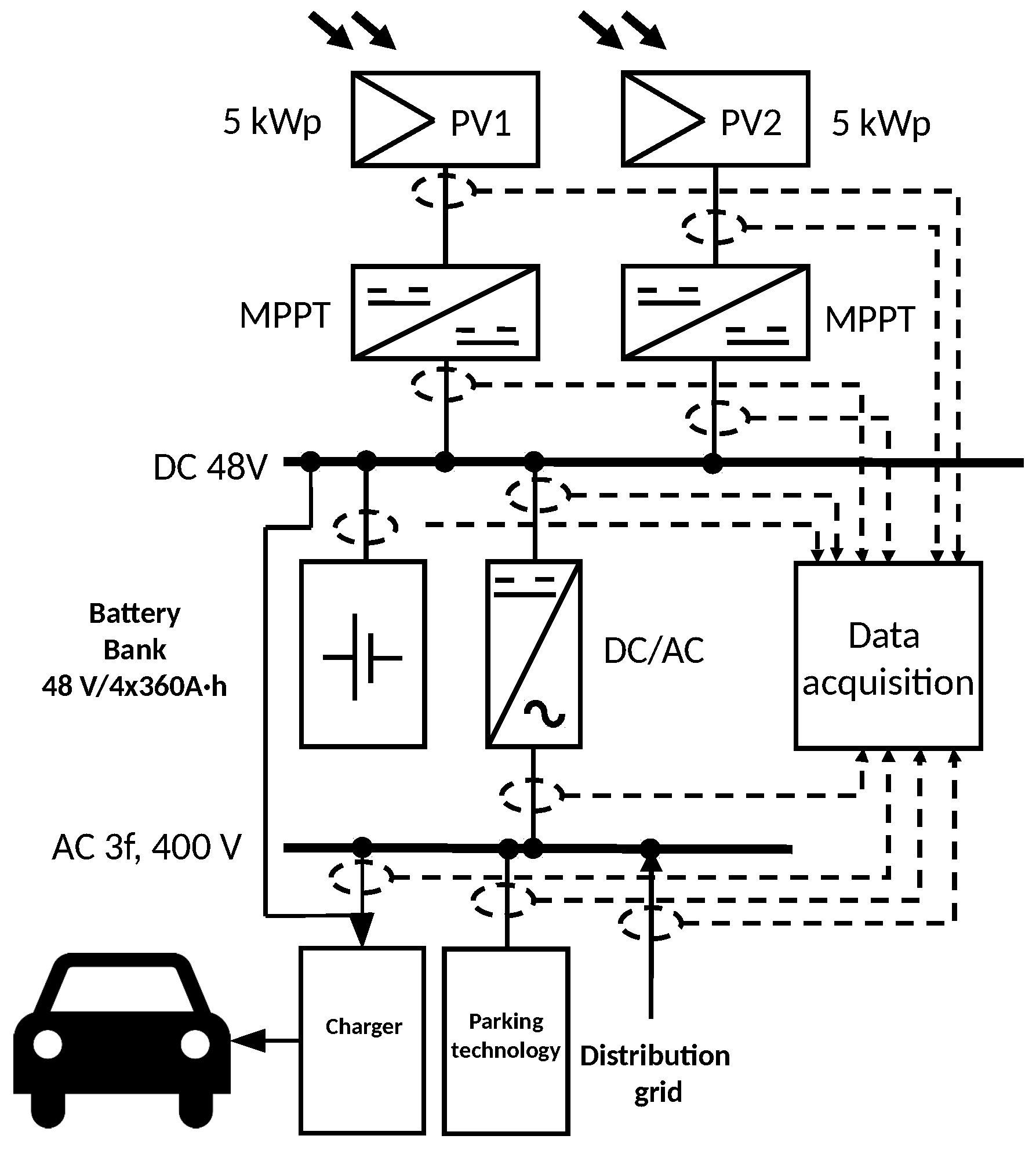
APSs are usually supplied from the low-voltage distribution network and to ensure a reliable operation, they are complemented with a backup power source, a diesel generator in the majority of cases. With regard to the trends in decentralised power generation, it is possible to use hybrid charging systems with DC coupling topology exploiting renewable energy resources and energy accumulation systems, thus eliminating the stochastic character of renewable energy supplies. APS presented herein is charged from a system complying with the characteristics mentioned above. The conceptual scheme of energy supply is shown in Figure 2.
3. Charge Schedule Optimization
The designed intelligent system managing the charge schedule in the automated multistory carpark contains several data-mining and machine learning techniques serving as supportive tools for the final decision making. The three layered structure is depicted in Figure 3.
The data managing part contains several kinds of sensors collecting information about moving cars, states of the system and current weather conditions. These data are grouped together with the historical data measured in the past and stored in a system’s database with additional user defined settings and system definitions. Based on statistical relevance for the given task, they are loaded, transformed and applied for the further step of performing the feature extraction.
The features relevant for the future plan optimization must at least represent a close approximation of a future progress of the described variable. The solar irradiation, closely related to the produced amount of energy by photovoltaic panels, is one of such variables. Its requirement is underlined by motivation to maximize the usage of energy gathered from renewable energy source.
The correct management of the charging plans needs the knowledge about future electric load and state of the car batteries. The energy demand estimation module takes care of this part, making use of the data definitions from database with real time sensor data.
The power quality, due to heavy loads of charges accompanied by the system’s low short-circuit power, may be volatile, which could negatively impact the quality of the charging process causing potential harm to the batteries. The power quality parameters predictions have been already addressed by our previous studies [11,32], but a different hardware setup with different loads requires new modeling of this aspect. PQP was not involved in this paper due to its preliminary character.
For each module, its inputs and outputs are described in further sections with the final charge schedule optimization performed by evolutionary based on MOO.
3.1. Solar Irradiation Forecasting
The module responsible for the forecasting of produced energy was based on statistical data preprocessing and regression based on an extreme learning machine algorithm [33,34]. This approach was already published and applied in our different research projects, therefore this section serves as a brief reminder in the context of this experiment.
The statistical preprocessing compounds the normalized weather data obtained from our measurements and also from weather forecasts, normalizes them into the common scale and calculates their relevance using mutual information estimation with Kraskov’s algorithm [35]. This approach confirmed that the highest relevance is possessed by variables describing the cloudiness on all levels. The normalized input values accompanied by their past values regarding their autocorrelation served as input values for the Extreme learning machine based regression. The details about the data, model and their adjustments may by found in [32,36]. The predictive accuracy was measured by Rooted Normalized Mean Square Error (RNMSE) where the average error of the forecast of the following 24 hours was approximately 28.57%.
The experiment proposed in this paper was performed on energy production data covering one year (four seasons) to include most weather variations in the region. The table describing the data according to the given month may be seen in Table 1.
3.2. Carpark Occupancy Monitoring
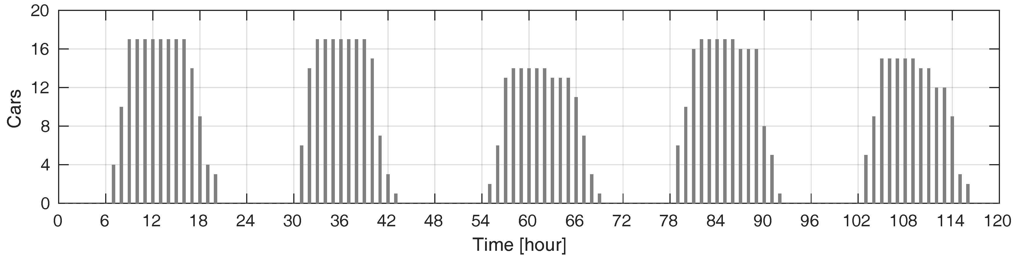
The multistory carpark occupancy data come from the survey of 20 employees from our institute. Their arrival and departure times were collected during a one month period with the information about travel distance to their homes. This was used to estimate the amount of required energy to be charged by the system when their cars are plugged in.
The occupancy data were transformed into time series, where each sample represented a number of cars that parked during a given 15 min period (see Figure 4). From these historical data, we were able to estimate the expected arrival and departure times for the following. The regular arrivals began from 5:45 a.m. to 11:45 a.m., with an average standard deviation of a car equaling to 32 min. The departures occurred in the interval from 12:30 p.m. to 9:45 p.m. with an average standard deviation of a car equaling to 75 min.
From these observations, we set that charging is not allowed 75 min before an estimated car departure and the batteries have to contain the defined amount of energy. In the case of a car being disconnected sooner by its owner, the car may not contain enough energy to sustain the entire trip home, but this is the user’s responsibility. We also defined the minimal waiting time for the charging after the car was plugged in after its parking. This time was set to 30 min to make the charging of the already connected cars more stable.
3.3. Electric Load Scenarios
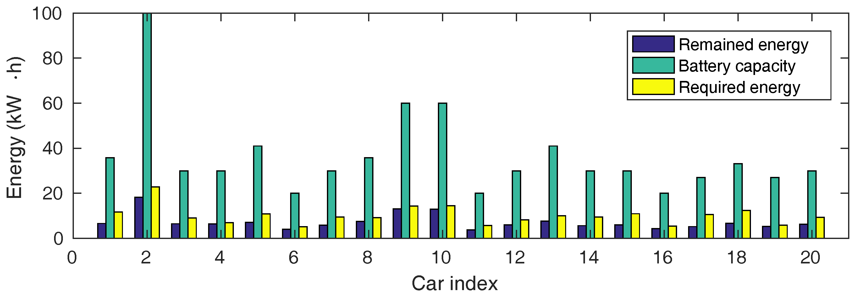
The electric load is defined by charging the cars parked inside and by consumption of the building itself. In this experiment, 20 EV were simulated with distribution based on available data describing sales of EV in Europe in 2017 [37] (see Table 2).
The amount of remaining energy of incoming car batteries was adjusted randomly with 20% mean and 15% standard deviation. The mandatory minimum to be charged was defined as the distance to driver’s home increased by an additional 25 km for any unexpected needs. The final amount was increased by an additional 50% to be prepared for worse weather conditions or other energy consuming circumstances. These constants for remained energy simulation were chosen with pessimism. The levels of batteries of each car may be seen in Figure 5, where the maximum capacity is accompanied by the current amount of energy as well as the desired energy to be charged. The final desired amount of energy was computed in two scenarios—the amount of energy with and without respect to the current battery level (final SoC was equal to the required SoC () or to the final SoC was decreased by current SoC ()).
To simulate the total demand and its progress, it is necessary to define a set of parameters describing the system. T is the number of time periods of the optimized day, where each period has an equal length of 15 min. N is the number of charging stations, represents the set of energy demands on all chargers at time t and states a set of produced energy at each time period. is the boolean matrix having true and false states for occupied and unoccupied parking slots respectively. The variable describes the current amount of energy in batteries limited by adjusted capacity .
Among the system parameters, the minimum electric load used for lightning and basic system maintenance per hour was adjusted to 800 W·h and the lift moving cars during their arrival or departure took 1.5 kW·h per car. The maximum energy supported by the system’s hardware is 21 kW·h. To compute the current demand d at the given time period t, the equation is defined as follows
where is the adjusted load of the i-th charger at time t and is calculated as the summation of arriving and leaving cars during time t multiplied by (1.5 kW·h). The maximum available energy for charging at time t is divided by four because t represents the 15 min time window.
Based on the number of cars, their arrival times and required levels of energy to charge, this model will produce different load vectors L, which will imply changes in total demand D altering the behavior of the entire system.
There were defined two different charge management algorithms to compare in this experiment. It is the simple come’n charge approach, where cars are consuming a maximum available amount of energy immediately after they are connected. This approach only checks the interconnection between car and grid and whether the battery is not already charged to the desired level. In this case, the load l of i-th charger at time t is defined as follows
where represents the charge demand of i-th car at time t. These demands may be estimated from previous iteration simply as
To drive the system’s demand towards our goals, we need to extend the model by additional parameters with ability to be optimized. They are the set of delayed starting charge times , which captures the index of time period when n-th car starts its charging and amount of energy that is used for the car during all its charging periods. The estimation of the load vector L is therefore extended from the Equation (2) into as follows
3.4. Optimized Charging
Previously involved adjustable parameter vectors A and B are evolutionary tuned to optimize the system during each given day. Three objective functions were defined to evaluate the feasibility of optimized solution and they are the minimum remaining amount of energy to be charged before the cars are going to leave (Equation (5)), the maximum usage of RES during the day period (Equation (6)) and the minimum amount of RES energy stored in the systems battery (Equation (7)). While the first two objectives may seems obvious, the minimization of is to minimize system’s inefficiency caused by 8% energy loss during each system’s battery charge.
Based on the given A and B, is simply computed as the sum of car demands at the final time period. The optimal solution will have equal to zero, meaning that all cars were charged to the desired level.
Objective functions and require simulating the energy flows between RES, system’s batteries and the charged cars. Therefore, we define the variable stating the amount of energy provided by RES and the vector representing the energy stored in the system batteries during each time period. This energy may serve for car charging in times when RES are insufficient. The algorithm simulating these flows may be seen in Algorithm 1. The main loop iterates through all time periods, where during each of them the produced energy is processed first. In lines 7–13, the algorithm tries to cover the energy demand by RES, while the rest of it is stored in the system’s battery. In cases when the production is insufficient, the demand is simply decreased by the amount of available RES energy (lines 15–16). The second part of the algorithm simulates covering the rest of demand by energy from the system’s batteries (lines 18–26). Maximum energy gain from these batteries is 95% of their capacity, which is also included in the algorithm. Variable also represents the necessary outcome of the procedure because the battery state from the previous day is carried into the following one to continue with the simulation.
| Algorithm 1: Pseudo-code of a function estimating the usage of RES and the total energy charged in the system’s battery |
 |
After Algorithm 1 is executed and variables and are computed, the and values were calculated as follows.
The optimal solution having equal to 0 represents the system that has worked only on RES—its maintenance was supported by system’s battery during the night and charging of the cars was mostly supported by RES. In case of , the ideal solution means the minimum energy flowed through the system’s batteries, therefore the system performed a minimum loss.
The problem based on three different objective functions required the application of the Multi-objective optimization approach. On the other hand, our objective functions were not equally important, which was further reflected by a modified candidate selection from the final Pareto front set.
3.5. Multi Objective Optimization
In general, the multi objective problem (MOP) is posed as an optimization problem of several (mostly conflicting) objective functions [38]. According to the defined equality and inequality constraints, the input value vector X defines the search space (often called a feasible design space) for solutions. MOO is mostly based on search-engine optimization, but there is one major difference from single-objective optimization. It is the number of solutions, which in the case of MOO is defined as a set of feasible solutions (called a Pareto Front). Each of its candidates is called Pareto Optimal, and together they form the so-called trade-off curve in a chart of objective values. The Pareto optimal solutions are randomly distributed on this curve reflecting their performance towards the defined objectives. The most suitable solution for the given application may be chosen by the fuzzy decision making process. User’s preferences towards a particular objective may be reflected by the adjustable weights used in this process.
3.5.1. Multi Objective Evolutionary Algorithm with Decomposition
(MOEA/D) [39] has become a vital member of MOO approaches over a longer period due to its successful applications and several derivatives. The main idea focuses on the decomposition of the MOP into the number of single objective optimization problems (SOP) to face them separately. Each SOP, so called a subproblem, is a (non)linear aggregation of defined objectives. The aggregations are also reflected in definition of neighborhoods among the subproblems solutions. The evolutionary algorithm may optimize the SOP, while for its inner operations it will use the closest neighbor’s solutions. This simplification allowed the application of other single optimization techniques to extend this approach in order to increase its performance. In several studies, this approach combined with Differential evolution [40] was able to outperform its ancestor, the NSGA-II [41]. This fact was also confirmed during our experiments, which is the main reason for using MOEA/D-DE for the optimization.
3.5.2. Differential Evolution
(DE) was developed by R. Storn and K. Price [42] and it possesses the features of a self-organizing search as well as an evolutionary based optimization. In general, DE is a heuristic mechanism driving the representative solutions, so called candidates through searched space to perform their optimization. DE offers several strategies driving the computation of new positions for its candidates. One of them takes three random candidates to calculate an intermediate candidate which creates a new position by binary crossover with an optimized candidate . It takes this new position only if it is better than the current one.
The mutation is handled by a selection of three random candidates (p, q, r) from the population and the so-called donor vector is calculated.
where is an adjustable hyper-parameter entitled as differential weight. From these statements, we can point out that minimal population size is .
The second hyper-parameter drives the crossover operation, which is performed between the computed donor vector and our evolving candidate.
The following fitness value calculation decides whether the new synthesized candidate will be kept instead of its ancestor or not.
3.5.3. Fuzzy Decision Making
The result of MOO forms the Pareto front set where the single feasible solution needs to be found. The selection of the most suitable candidate is frequently ensured by a fuzzy decision making process having calculated the linear membership function for all members of the Pareto Front. In [11,43], the objective function to be minimized, the membership function follows below:
Accordingly, the objective function to be maximized, the definition is given below:
where and are the minimal and maximal value of objective function from the payoff table (), is the value of ith objective function of rth Pareto Front member and is its membership value for ith objective function. During calculation of the total membership value of the rth Pareto Front member, we are able to apply membership weights for each of the objective function as it is defined below:
which enables us to control the importance of the membership values for each of the objective functions separately.
The payoff table is a squared matrix containing the normalized values of objective functions when each of them was optimized separately by some single objective approach. The best objective function values represent the position of U, the so called utopia point—the best possible solution and the worst objective function values represent N—nadir point, or the worst possible solution. The best trade-off solution is placed the nearest to the U. In some cases, the single objective optimizations obtaining payoff table does not have to be involved. In order to reduce the computational complexity, the utopia and nadir points are estimated as the best and worst obtained values from the normalized objective function values of Pareto front.
According to the adjusted preferences, the final solution may be selected for further application. In our case, the fuzzy decision process was engaged only on Pareto front members having zero amount of energy to be charged (). Fulfillment of this condition was considered as necessary.
4. Simulations and Results
Based on previous definitions, the optimization of the charging mechanism towards the defined criteria (Equations (5)–(7)) was achieved by evolutionary tuning of the parameter vectors A and B. The candidate of MOEA/D-DE population was simply the vector of real numbers in range [0–1] having length of these parameter vectors combined. While the A parameters were directly applied in the model, B values were multiplied by T and floored to correctly represent the time periods.
The final adjustment of MOO followed the similar manners as its previous applications [11] and it was also performed experimentally to obtain some optimal convergence. The number of candidates was adjusted according to the dimension of the optimized problem, while the number of evaluations was kept reasonably high to perform a valid search. Table 3 describes the parameters of the optimization process and their values. The implementation of the entire experiment was in the MATLAB environment making use the PLATEMO package [44] with some additional data processing, evaluation and visualization techniques.
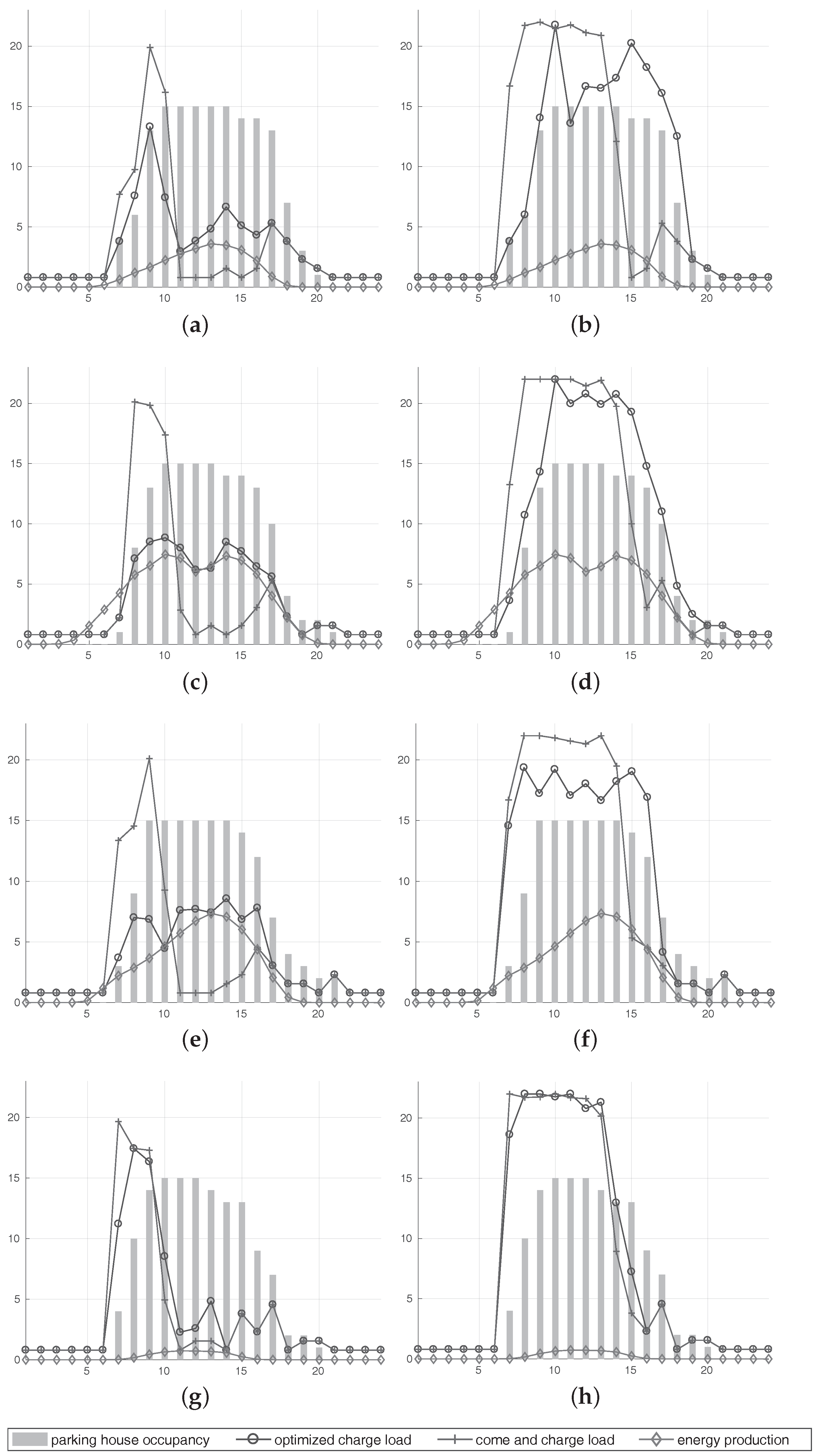
This algorithm simply took current battery state (), the 24-h ahead forecasting of energy production (P) and occupancy data (C) tested on the given date and performed the energy consumption optimization to fit the given goals. This new consumption plan was evaluated and the new battery state was derived for the following day, when optimization was repeated. The examples on four different days may be seen in Figure 6. In cases of higher RES production and lower energy demand defined by scenario, the optimization was able to cover the most of the demand by RES, which minimized the energy loss and maximized the RES use. In other cases, the higher desire of RES use only shifted the charging process a few time periods further. In cases when RES was very low, the optimization performed almost no change.
Table 4 and Table 5 contain the evaluations of simulated optimizations on the given data. The usage of RES and the percentage of energy load covered by RES were compared on different battery setups, where each of them ran in an optimized and unoptimized mode. Table 4 reflects the results using the scenario with a higher load (), while Table 5 describes charging cars regarding their current battery state (). In cases when RES produced a significant amount of energy, the optimization was able to outperform the unoptimized setup with a larger battery set. In other cases, RES production was always fully consumed and further optimization was not logically able to improve it. Comparing the amounts of saved energy among Table 4 and Table 5, we can see that the increasing by a higher recharging level also increases the necessity of higher load from the grid. The cost efficiency is compared in the following tables.
The system’s behavior also significantly differs based on the two load scenarios. While in , the differences in energy efficiency clearly appeared, in did not. This is caused by a lower energy production that is not able to fully support , therefore it will never be able to cover a major part of its consumption.
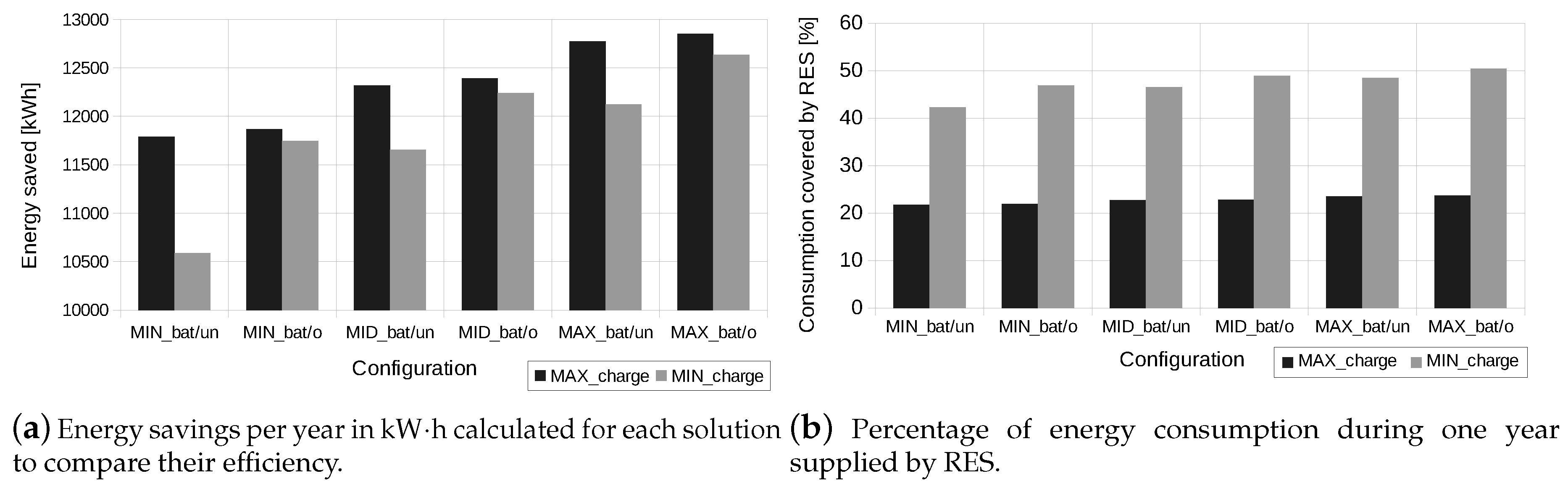
Table 6 and Table 7, and Figure 7a summarize the total amount of energy saved in both load scenarios and all simulated configurations during the year. As we can see, the differences in energy savings between load scenarios are rather minimal. It implies that scenario is able to perform more than double energy efficiency compared to (see Figure 7b).
As we can see, the higher energy demand in scenario did not significantly increase the usage of RES due to limited and variable supply from this source. On the other hand, this higher demand was necessary to cover for On-Grid supply, which increased the operational costs of the solution. The difference in energy savings among the battery setups in this scenario was rather minimal. It was caused by the mentioned high energy demand consuming the entire RES supply almost equally.
In case of scenario, the energy from RES covered more than 50% of the total consumption in most cases. Our optimization was able to increase the RES usage by 5–10% depending on the given month, which is considered a valid result. Some differences among the battery setups appeared, such as that those a with higher capacity were able to be re-charged during the weekend when multistory carpark was unoccupied and thus served as additional RES. One of the most interesting outcomes is the fact that energy efficiency obtained by any bigger battery setup was always outperformed by smaller battery setup extended by our optimization. This fact may serve as valuable information when a low-cost solution is being developed.
The best results in general were obtained during summer months, when the solar irradiation achieved its peak. The optimization performed almost no improvement during winter months, when RES supply represented less than 10% of the total energy consumption.
5. Conclusions
Adaptive charge management supported by MOO was proposed and evaluated in this paper. Three different battery setups and two charging scenarios were examined over a one-year period to maximize the completeness of experiment. The main outcome of this paper is the shape of the trade-off curve among the conflicting criteria that may be given to the similar system. They may be the purchase price, operational costs, energy efficiency and user comfort. As it was described, the higher user comfort ( and ) may double the operational costs due to a 300% increase in the purchase price, while the total amount of RES use remains almost similar to the significantly cheaper solution. As a reward, the cars are charged on a much higher SoC level. This information may help during the design of a new solution reflecting the current financial abilities and user’s preferences. Due to the sufficient results, our future work aims to decrease the computational time, which is necessary for timely reactions of the system. This solution was able to synthesize a new charge scenario in 2–3 min, which may be decreased using parallel computing or evolutionary optimization enhanced with memory [45].
Author Contributions
Conceptualization, L.P.; Data curation, T.V.; Funding acquisition, L.P.; Methodology, T.V.; Project administration, L.P. and S.M.; Resources, S.M.; Software, T.V.; Supervision, L.P. and S.M.; Validation, T.V.; Visualization, T.V.; Writing—original draft, L.P. and T.V.; Writing—review & editing, S.M.
Acknowledgments
This paper was supported by the following projects: LO1404: Sustainable development of ENET Centre; CZ.1.05/2.1.00/19.0389 Development of the ENET Centre research infrastructure; SP2018/58 Students Grant Competition and TACR TH01020426, Czech Republic and the Project LTI17023 "Energy Research and Development Information Centre of the Czech Republic" funded by Ministry of Education, Youth and Sports of the Czech Republic, program INTER-EXCELLENCE, subprogram INTER-INFORM.
Conflicts of Interest
The authors declare no conflict of interest.
References
- Recast, E. Directive 2010/31/EU of the European Parliament and of the Council of 19 May 2010 on the energy performance of buildings (recast). Off. J. Eur. Union 2010, 18, 2010. [Google Scholar]
- Van Roy, J.; Leemput, N.; De Breucker, S.; Geth, F.; Tant, P.; Driesen, J. An availability analysis and energy consumption model for a flemish fleet of electric vehicles. In Proceedings of the European Electric Vehicle Congress (EEVC), Brussels, Belgium, 26–28 October 2011. [Google Scholar]
- Sortomme, E.; Hindi, M.M.; MacPherson, S.J.; Venkata, S. Coordinated charging of plug-in hybrid electric vehicles to minimize distribution system losses. IEEE Trans. Smart Grid 2011, 2, 198–205. [Google Scholar] [CrossRef]
- Clement-Nyns, K.; Haesen, E.; Driesen, J. The impact of charging plug-in hybrid electric vehicles on a residential distribution grid. IEEE Trans. Power Syst. 2010, 25, 371–380. [Google Scholar] [CrossRef] [Green Version]
- Zhang, K.; Xu, L.; Ouyang, M.; Wang, H.; Lu, L.; Li, J.; Li, Z. Optimal decentralized valley-filling charging strategy for electric vehicles. Energy Conv. Manag. 2014, 78, 537–550. [Google Scholar] [CrossRef]
- Cao, Y.; Tang, S.; Li, C.; Zhang, P.; Tan, Y.; Zhang, Z.; Li, J. An optimized EV charging model considering TOU price and SOC curve. IEEE Trans. Smart Grid 2012, 3, 388–393. [Google Scholar] [CrossRef]
- Korolko, N.; Sahinoglu, Z. Robust optimization of EV charging schedules in unregulated electricity markets. IEEE Trans. Smart Grid 2017, 8, 149–157. [Google Scholar] [CrossRef]
- Jin, C.; Tang, J.; Ghosh, P. Optimizing electric vehicle charging with energy storage in the electricity market. IEEE Trans. Smart Grid 2013, 4, 311–320. [Google Scholar] [CrossRef]
- Vayá, M.G.; Andersson, G. Optimal bidding strategy of a plug-in electric vehicle aggregator in day-ahead electricity markets under uncertainty. IEEE Trans. Power Syst. 2015, 30, 2375–2385. [Google Scholar] [CrossRef]
- Slanina, Z.; Dedek, J.; Golembiovsky, M. Low Cost Battery Management System. J. Telecommun. Electron. Comput. Eng. 2017, 9, 87–90. [Google Scholar]
- Vantuch, T.; Mišák, S.; Ježowicz, T.; Buriánek, T.; Snášel, V. The power quality forecasting model for off-grid system supported by multiobjective optimization. IEEE Trans. Ind. Electron. 2017, 64, 9507–9516. [Google Scholar] [CrossRef]
- Allard, S.; See, P.C.; Molinas, M.; Fosso, O.B.; Foosnas, J.A. Electric vehicles charging in a smart microgrid supplied with wind energy. In Proceedings of the 2013 IEEE Grenoble Conference, Grenoble, France, 16–20 June 2013; pp. 1–5. [Google Scholar]
- Huang, Q.; Jia, Q.S.; Qiu, Z.; Guan, X.; Deconinck, G. Matching EV charging load with uncertain wind: A simulation-based policy improvement approach. IEEE Trans. Smart Grid 2015, 6, 1425–1433. [Google Scholar] [CrossRef]
- Wu, D.; Aliprantis, D.C.; Ying, L. Load scheduling and dispatch for aggregators of plug-in electric vehicles. IEEE Trans. Smart Grid 2012, 3, 368–376. [Google Scholar] [CrossRef]
- Slanina, Z.; Docekal, T. Energy monitoring and managing for electromobility purposes. In Proceedings of the Photonics Applications in Astronomy, Communications, Industry, and High-Energy Physics Experiments 2016, Wilga, Poland, 28 September 2016; Volume 10031, p. 100311P. [Google Scholar]
- You, P.; Yang, Z.; Chow, M.Y.; Sun, Y. Optimal cooperative charging strategy for a smart charging station of electric vehicles. IEEE Trans. Power Syst. 2016, 31, 2946–2956. [Google Scholar] [CrossRef]
- Vayá, M.G.; Andersson, G.; Boyd, S. Decentralized control of plug-in electric vehicles under driving uncertainty. In Proceedings of the 2014 IEEE PES Innovative Smart Grid Technologies Conference Europe (ISGT-Europe), Istanbul, Turkey, 12–15 October 2014; pp. 1–6. [Google Scholar]
- He, Y.; Venkatesh, B.; Guan, L. Optimal scheduling for charging and discharging of electric vehicles. IEEE Trans. Smart Grid 2012, 3, 1095–1105. [Google Scholar] [CrossRef]
- Rivera, J.; Goebel, C.; Jacobsen, H.A. Distributed convex optimization for electric vehicle aggregators. IEEE Trans. Smart Grid 2017, 8, 1852–1863. [Google Scholar] [CrossRef]
- Rotering, N.; Ilic, M. Optimal charge control of plug-in hybrid electric vehicles in deregulated electricity markets. IEEE Trans. Power Syst. 2011, 26, 1021–1029. [Google Scholar] [CrossRef]
- Shaaban, M.F.; Atwa, Y.M.; El-Saadany, E.F. PEVs modeling and impacts mitigation in distribution networks. IEEE Trans. Power Syst. 2013, 28, 1122–1131. [Google Scholar] [CrossRef]
- Valentine, K.; Temple, W.G.; Zhang, K.M. Intelligent electric vehicle charging: Rethinking the valley-fill. J. Power Sources 2011, 196, 10717–10726. [Google Scholar] [CrossRef]
- El-Zonkoly, A.; dos Santos Coelho, L. Optimal allocation, sizing of PHEV parking lots in distribution system. Int. J. Electr. Power Energy Syst. 2015, 67, 472–477. [Google Scholar] [CrossRef]
- Yang, Z.; Li, K.; Foley, A. Computational scheduling methods for integrating plug-in electric vehicles with power systems: A review. Renew. Sustain. Energy Rev. 2015, 51, 396–416. [Google Scholar] [CrossRef]
- Mukherjee, J.C.; Gupta, A. A review of charge scheduling of electric vehicles in smart grid. IEEE Syst. J. 2015, 9, 1541–1553. [Google Scholar] [CrossRef]
- Prokop, L.; Vantuch, T.; Misak, S. Automated Parking System Supplied by Off-Grid Power System with an Intelligent Control System. In Proceedings of the 9th International Scientific Symposium on Electrical Power Engineering, ELEKTROENERGETIKA 2017, Stara Lesna, Slovakia, 12–14 September 2017; pp. 489–493. [Google Scholar]
- Yilmaz, M.; Krein, P.T. Review of the impact of vehicle-to-grid technologies on distribution systems and utility interfaces. IEEE Trans. Power Electron. 2013, 28, 5673–5689. [Google Scholar] [CrossRef]
- KOMA TOWER—KOMA Parking. Available online: http://www.komaparking.cz/koma-tower-en/ (accessed on 25 May 2018).
- Bauer, P.; Weldemariam, L.E.; Raijen, E. Stand-alone microgrids. In Proceedings of the 2011 IEEE 33rd International Telecommunications Energy Conference (INTELEC), Amsterdam, The Netherlands, 9–13 October 2011; pp. 1–10. [Google Scholar]
- Ustun, T.S.; Ozansoy, C.R.; Zayegh, A. Implementing vehicle-to-grid (V2G) technology with IEC 61850-7-420. IEEE Trans. Smart Grid 2013, 4, 1180–1187. [Google Scholar] [CrossRef]
- Quílez, M.G.; Abdel-Monem, M.; Baghdadi, M.E.; Yang, Y.; Van Mierlo, J.; Hegazy, O. Modelling, Analysis and Performance Evaluation of Power Conversion Unit in G2V/V2G Application—A Review. Energies 2018, 11, 1082. [Google Scholar] [CrossRef]
- Misak, S.; Stuchly, J.; Vantuch, T.; Burianek, T.; Seidl, D.; Prokop, L. A holistic approach to power quality parameter optimization in AC coupling Off-Grid systems. Electr. Power Syst. Res. 2017, 147, 165–173. [Google Scholar] [CrossRef]
- Huang, G.B.; Zhu, Q.Y.; Siew, C.K. Extreme learning machine: Theory and applications. Neurocomputing 2006, 70, 489–501. [Google Scholar] [CrossRef] [Green Version]
- Huang, G.B. What are Extreme Learning Machines? Filling the Gap Between Frank Rosenblatt’s Dream and John von Neumann’s Puzzle. Cogn. Comput. 2015, 7, 263–278. [Google Scholar] [CrossRef]
- Kraskov, A.; Stögbauer, H.; Grassberger, P. Estimating mutual information. Phys. Rev. E 2004, 69, 066138. [Google Scholar] [CrossRef] [PubMed]
- Burianek, T.; Misak, S. Solar irradiance forecasting model based on extreme learning machine. In Proceedings of the 2016 IEEE 16th International Conference on Environment and Electrical Engineering (EEEIC), Florence, Italy, 7–10 June 2016; pp. 1–5. [Google Scholar]
- EVObsession: 2017 Electric Car Sales—US, China, and Europe. Available online: https://evobsession.com/2017-electric-car-sales-us-china-europe-month-month/ (accessed on 25 May 2018).
- Deb, K. Multi-Objective Optimization Using Evolutionary Algorithms; John Wiley & Sons: New York, NY, USA, 2001; Volume 16. [Google Scholar]
- Zhang, Q.; Li, H. MOEA/D: A multiobjective evolutionary algorithm based on decomposition. IEEE Trans. Evol. Comput. 2007, 11, 712–731. [Google Scholar] [CrossRef]
- Li, H.; Zhang, Q. Multiobjective optimization problems with complicated Pareto sets, MOEA/D and NSGA-II. IEEE Trans. Evol. Comput. 2009, 13, 284–302. [Google Scholar] [CrossRef]
- Deb, K.; Pratap, A.; Agarwal, S.; Meyarivan, T. A fast and elitist multiobjective genetic algorithm: NSGA-II. IEEE Trans. Evol. Comput. 2002, 6, 182–197. [Google Scholar] [CrossRef] [Green Version]
- Storn, R.; Price, K. Differential evolution–a simple and efficient heuristic for global optimization over continuous spaces. J. Glob. Optim. 1997, 11, 341–359. [Google Scholar] [CrossRef]
- Aghaei, J.; Amjady, N.; Shayanfar, H.A. Multi-objective electricity market clearing considering dynamic security by lexicographic optimization and augmented epsilon constraint method. Appl. Soft Comput. 2011, 11, 3846–3858. [Google Scholar] [CrossRef]
- Tian, Y.; Cheng, R.; Zhang, X.; Jin, Y. PlatEMO: A MATLAB Platform for Evolutionary Multi-Objective Optimization [Educational Forum]. IEEE Comput. Intell. Mag. 2017, 12, 73–87. [Google Scholar] [CrossRef]
- Wang, Y.; Li, B. Investigation of memory-based multi-objective optimization evolutionary algorithm in dynamic environment. In Proceedings of the 2009 IEEE Congress on Evolutionary Computation, Trondheim, Norway, 18–21 May 2009; pp. 630–637. [Google Scholar]
Figure 1.
A view of APS; APS skeleton.

Figure 2.
Scheme of the automated parking system.

Figure 3.
A UML diagram of an intelligent decision making system controlling the charge schedule in automated multistory carpark.
Figure 3.
A UML diagram of an intelligent decision making system controlling the charge schedule in automated multistory carpark.
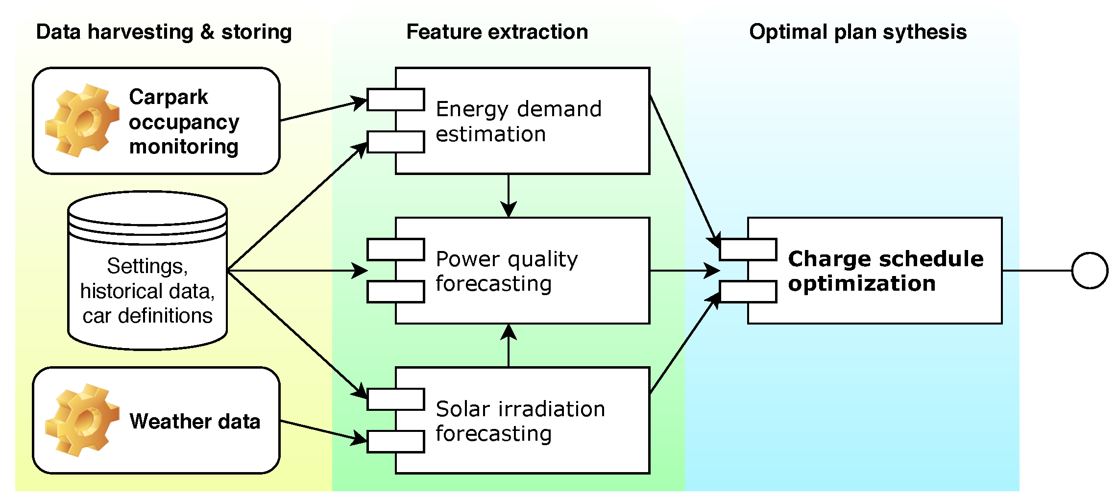
Figure 4.
Multistory carpark occupancy on a week scale.

Figure 5.
Distribution of energy remained and required per car given for the charge optimization.

Figure 6.
The comparisons of optimized loads vs. come’n charge loads on four different months ((a,b) March, (c,d) June, (e,f) September and (g,h) December) and both consumption modes ((a,c,e,f) reflect consumption lowered by the current battery state while (b,d,f,h) are not taking this into account). In all figures, the horizontal axis represents time in hours (1 day) and vertical axis means the absolute values of depicted measures (number of cars and kW·h).

Figure 7.
Comparison of different battery setups and charging scenarios on a year-long simulation.


Table 1.
Statistical features of predicted energy production during selected months.
| Month | Min-Max kW·h at 12’ | Max/Day [kW·h] | Min/Day [kW·h] | Std/ Day [kW·h] | Total [kW·h] |
|---|---|---|---|---|---|
| February | 0.94–3.36 | 21.30 | 5.70 | 4.44 | 369.91 |
| April | 1.84–7.51 | 67.17 | 16.77 | 13.85 | 1351.59 |
| July | 4.86–9.56 | 90.71 | 41.78 | 15.66 | 2224.11 |
| October | 1.28–3.88 | 27.87 | 9.58 | 3.44 | 469.25 |
Table 2.
Electric vehicles used in this experiment with approximated probabilities according to their selling distribution in Europe during 2017 [37].
Table 2.
Electric vehicles used in this experiment with approximated probabilities according to their selling distribution in Europe during 2017 [37].
| Car | Driving Distance [km] | Battery Capacity [kW·h] | Probability |
|---|---|---|---|
| Nissan LEAF | 200 | 30 | 0.17 |
| Volkswagen Golf | 300 | 35.8 | 0.12 |
| Volkswagen e-up! | 160 | 20 | 0.03 |
| BMW i3 | 200 | 33.2 | 0.19 |
| Tesla X | 565 | 100 | 0.12 |
| Opel Ampera | 520 | 60 | 0.03 |
| Renault ZOE | 400 | 41 | 0.30 |
| Kia Soul EV | 250 | 27 | 0.05 |
Table 3.
Settings for MOEA/D-DE algorithm.
| Parameter | Value |
|---|---|
| applied algorithm | MOEA-DDE |
| size of population | 80 |
| number of iterations | 20,000 |
| —probability of choosing parents locally | 0.9 |
| —number of solutions replaced by each offspring | 2 |
| —crossover probability | 1 |
| F—differential weight | 0.5 |
| —expected number of bits doing mutation | 1 |
| —distribution index of polynomial mutation | 20 |
Table 4.
Energy savings acquired for different system configurations having optimized and unoptimized simulations. Shortcut ’ru’ means percentage of renewable energy used and ’cl’ means the percentage of covered load by RES. Outcomes in this table were computed on lower charging scenario—not taking the current battery balance in car.
| Mon. | Total FVE Production [kW] | Total Consumption [kW/Month] | MIN BAT [23.04 kW·h] | MID BAT [46.08 kW·h] | MAX BAT [69.12 kW·h] | |||||||||
|---|---|---|---|---|---|---|---|---|---|---|---|---|---|---|
| Unoptimized | Optimized | Unoptimized | Optimized | Unoptimized | Optimized | |||||||||
| ru | cl | ru | cl | ru | cl | ru | cl | ru | cl | ru | cl | |||
| Jan. | 265.91 | 4701.30 | 99.18 | 5.61 | 99.29 | 5.62 | 99.18 | 5.61 | 99.29 | 5.62 | 99.18 | 5.61 | 99.29 | 5.62 |
| Feb. | 369.91 | 4112.83 | 98.66 | 8.87 | 98.88 | 8.89 | 98.66 | 8.87 | 98.88 | 8.89 | 98.66 | 8.87 | 98.88 | 8.89 |
| Mar. | 800.41 | 4481.71 | 95.65 | 17.08 | 95.94 | 17.13 | 98.24 | 17.54 | 98.53 | 17.60 | 99.11 | 17.70 | 99.40 | 17.75 |
| Apr. | 1351.59 | 4494.72 | 87.90 | 26.43 | 88.21 | 26.53 | 93.21 | 28.03 | 93.52 | 28.12 | 97.81 | 29.41 | 98.12 | 29.51 |
| May | 2079.81 | 4757.97 | 85.08 | 37.19 | 85.85 | 37.53 | 89.29 | 39.03 | 90.06 | 39.37 | 93.43 | 40.84 | 94.20 | 41.18 |
| Jun. | 2452.42 | 4328.86 | 77.03 | 43.64 | 77.91 | 44.19 | 80.60 | 45.66 | 81.48 | 46.22 | 84.17 | 47.69 | 85.04 | 48.24 |
| Jul. | 2224.05 | 4537.53 | 81.66 | 40.03 | 82.32 | 40.35 | 86.58 | 42.44 | 87.24 | 42.76 | 90.96 | 44.58 | 91.61 | 44.90 |
| Aug. | 1965.37 | 4703.49 | 85.03 | 35.53 | 85.51 | 35.73 | 89.48 | 37.39 | 89.96 | 37.59 | 93.81 | 39.20 | 94.29 | 39.40 |
| Sep. | 1277.16 | 4517.54 | 89.69 | 25.36 | 90.05 | 25.46 | 94.54 | 26.73 | 94.91 | 26.83 | 97.01 | 27.43 | 97.38 | 27.53 |
| Oct. | 467.60 | 4520.50 | 98.81 | 10.22 | 98.33 | 10.21 | 98.81 | 10.22 | 98.33 | 10.21 | 98.81 | 10.22 | 98.33 | 10.21 |
| Nov. | 266.78 | 4328.86 | 99.26 | 6.12 | 99.23 | 6.12 | 99.26 | 6.12 | 99.23 | 6.12 | 99.26 | 6.12 | 99.23 | 6.12 |
| Dec. | 189.70 | 4681.86 | 99.66 | 4.04 | 99.68 | 4.04 | 99.66 | 4.04 | 99.68 | 4.04 | 99.66 | 4.04 | 99.68 | 4.04 |
Table 5.
Energy savings acquired for different system configurations having optimized and unoptimized simulations. Shortcut ’ru’ means percentage of renewable energy used and ’cl’ means the percentage of covered load by RES. Outcomes in this table were computed on lower charging scenario—taking the current battery balance in car.
| Mon. | total FVE Production [kW] | Total Consumption [kW/month] | MIN BAT [23.04 kW·h] | MID BAT [46.08 kW·h] | MAX BAT [69.12 kW·h] | |||||||||
|---|---|---|---|---|---|---|---|---|---|---|---|---|---|---|
| Unoptimized | Optimized | Unoptimized | Optimized | Unoptimized | Optimized | |||||||||
| ru | cl | ru | cl | ru | cl | ru | cl | ru | cl | ru | cl | |||
| Jan. | 265.91 | 2166.49 | 97.85 | 12.01 | 99.29 | 12.19 | 97.85 | 12.01 | 99.29 | 12.19 | 97.85 | 12.01 | 99.29 | 12.19 |
| Feb. | 369.91 | 1904.68 | 96.97 | 18.83 | 98.88 | 19.20 | 96.97 | 18.83 | 98.88 | 19.20 | 96.97 | 18.83 | 98.88 | 19.20 |
| Mar. | 800.41 | 2070.50 | 91.35 | 35.31 | 95.89 | 37.07 | 93.94 | 36.31 | 98.50 | 38.08 | 95.48 | 36.91 | 99.38 | 38.42 |
| Apr. | 1351.59 | 2075.92 | 82.78 | 53.89 | 87.97 | 57.28 | 89.41 | 58.21 | 93.35 | 60.78 | 94.26 | 61.37 | 97.90 | 63.74 |
| May | 2079.81 | 2185.61 | 74.80 | 71.18 | 85.21 | 81.10 | 84.89 | 80.78 | 89.45 | 85.13 | 89.10 | 84.78 | 93.49 | 88.98 |
| Jun. | 2452.42 | 2010.37 | 64.82 | 79.07 | 75.74 | 92.51 | 74.17 | 90.48 | 78.75 | 96.18 | 77.49 | 94.53 | 80.86 | 98.76 |
| Jul. | 2224.05 | 2099.77 | 68.17 | 72.21 | 80.71 | 85.48 | 79.50 | 84.21 | 83.78 | 88.75 | 82.69 | 87.58 | 86.19 | 91.30 |
| Aug. | 1965.37 | 2162.35 | 74.96 | 68.13 | 84.97 | 77.23 | 84.00 | 76.35 | 90.43 | 82.19 | 89.54 | 81.38 | 95.64 | 86.93 |
| Sep. | 1277.16 | 2076.15 | 84.67 | 52.08 | 89.86 | 55.28 | 91.57 | 56.33 | 94.77 | 58.30 | 94.93 | 58.39 | 97.58 | 60.02 |
| Oct. | 467.60 | 2097.75 | 96.90 | 21.60 | 98.33 | 21.99 | 96.90 | 21.60 | 98.33 | 21.99 | 96.90 | 21.60 | 98.32 | 21.99 |
| Nov. | 266.78 | 2010.37 | 97.75 | 12.97 | 99.23 | 13.17 | 97.75 | 12.97 | 99.23 | 13.17 | 97.75 | 12.97 | 99.23 | 13.17 |
| Dec. | 189.70 | 2156.95 | 98.94 | 8.70 | 99.68 | 8.77 | 98.94 | 8.70 | 99.68 | 8.77 | 98.94 | 8.70 | 99.68 | 8.77 |
Table 6.
Monthly energy savings in kWh calculated for each solution to compare their efficiency applying scenario. SUM represents the total saving of the given solution during the year.
Table 6.
Monthly energy savings in kWh calculated for each solution to compare their efficiency applying scenario. SUM represents the total saving of the given solution during the year.
| Mon. | MIN BAT [23.04 kW·h] | MID BAT [46.08 kW·h] | MAX BAT [69.12 kW·h] | |||
|---|---|---|---|---|---|---|
| Unoptimized | Optimized | Unoptimized | Optimized | Unoptimized | Optimized | |
| Jan. | 260.20 | 264.10 | 260.20 | 264.10 | 260.20 | 264.10 |
| Feb. | 358.65 | 365.70 | 358.65 | 365.70 | 358.65 | 365.70 |
| Mar. | 731.09 | 767.53 | 751.80 | 788.45 | 764.22 | 795.49 |
| Apr. | 1118.71 | 1189.09 | 1208.39 | 1261.74 | 1273.99 | 1323.19 |
| May | 1555.72 | 1772.53 | 1765.54 | 1860.61 | 1852.96 | 1944.76 |
| Jun. | 1589.60 | 1859.79 | 1818.98 | 1933.57 | 1900.40 | 1985.44 |
| Jul. | 1516.24 | 1794.88 | 1768.22 | 1863.55 | 1838.98 | 1917.09 |
| Aug. | 1473.21 | 1669.98 | 1650.95 | 1777.24 | 1759.72 | 1879.73 |
| Sep. | 1081.26 | 1147.70 | 1169.50 | 1210.40 | 1212.26 | 1246.11 |
| Oct. | 453.11 | 461.30 | 453.11 | 461.30 | 453.11 | 461.30 |
| Nov. | 260.74 | 264.77 | 260.74 | 264.77 | 260.74 | 264.77 |
| Dec. | 187.65 | 189.16 | 187.65 | 189.16 | 187.65 | 189.16 |
| SUM | 10,586.20 | 11,746.53 | 11,653.74 | 12,240.57 | 12,122.90 | 12,636.82 |
| DIFF | = | 1160.33 | 1067.54 | 1654.37 | 1536.70 | 2050.62 |
Table 7.
Monthly energy savings in kWh calculated for each solution to compare their efficiency applying scenario. SUM represents the total savings of the given solution during the year.
Table 7.
Monthly energy savings in kWh calculated for each solution to compare their efficiency applying scenario. SUM represents the total savings of the given solution during the year.
| Mon. | MIN BAT [23.04 kW·h] | MID BAT [46.08 kW·h] | MAX BAT [69.12 kW·h] | |||
|---|---|---|---|---|---|---|
| Unoptimized | Optimized | Unoptimized | Optimized | Unoptimized | Optimized | |
| Jan. | 263.74 | 264.21 | 263.74 | 264.21 | 263.74 | 264.21 |
| Feb. | 364.81 | 365.63 | 364.81 | 365.63 | 364.81 | 365.63 |
| Mar. | 765.48 | 767.72 | 786.09 | 788.78 | 793.26 | 795.50 |
| Apr. | 1187.95 | 1192.45 | 1259.87 | 1263.92 | 1321.90 | 1326.39 |
| May | 1769.49 | 1785.67 | 1857.04 | 1873.21 | 1943.15 | 1959.33 |
| Jun. | 1889.11 | 1912.92 | 1976.56 | 2000.80 | 2064.43 | 2088.24 |
| Jul. | 1816.37 | 1830.89 | 1925.73 | 1940.25 | 2022.83 | 2037.35 |
| Aug. | 1671.15 | 1680.56 | 1758.63 | 1768.04 | 1843.77 | 1853.18 |
| Sep. | 1145.65 | 1150.17 | 1207.54 | 1212.06 | 1239.16 | 1243.68 |
| Oct. | 462.00 | 461.54 | 462.00 | 461.54 | 462.00 | 461.54 |
| Nov. | 264.93 | 264.93 | 264.93 | 264.93 | 264.93 | 264.93 |
| Dec. | 189.15 | 189.15 | 189.15 | 189.15 | 189.15 | 189.15 |
| SUM | 11,789.82 | 11,865.83 | 12,316.08 | 12,392.51 | 12,773.13 | 12,849.13 |
| DIFF | = | 76.00 | 526.25 | 602.68 | 983.30 | 1059.30 |
© 2018 by the authors. Licensee MDPI, Basel, Switzerland. This article is an open access article distributed under the terms and conditions of the Creative Commons Attribution (CC BY) license (http://creativecommons.org/licenses/by/4.0/).
Share and Cite
MDPI and ACS Style
Prokop, L.; Vantuch, T.; Mišák, S. Multi Objective Optimization in Charge Management of Micro Grid Based Multistory Carpark. Energies 2018, 11, 1791. https://doi.org/10.3390/en11071791
AMA Style
Prokop L, Vantuch T, Mišák S. Multi Objective Optimization in Charge Management of Micro Grid Based Multistory Carpark. Energies. 2018; 11(7):1791. https://doi.org/10.3390/en11071791
Chicago/Turabian StyleProkop, Lukáš, Tomáš Vantuch, and Stanislav Mišák. 2018. "Multi Objective Optimization in Charge Management of Micro Grid Based Multistory Carpark" Energies 11, no. 7: 1791. https://doi.org/10.3390/en11071791
Note that from the first issue of 2016, this journal uses article numbers instead of page numbers. See further details here.