The Effect of Fractional Orders on the Transmission Power and Efficiency of Fractional-Order Wireless Power Transmission System

School of Electric Power Engineering, South China University of Technology, Guangzhou 510641, China
*
Author to whom correspondence should be addressed.
Energies 2018, 11(7), 1774; https://doi.org/10.3390/en11071774
Submission received: 26 May 2018
/
Revised: 20 June 2018
/
Accepted: 2 July 2018
/
Published: 6 July 2018
(This article belongs to the Special Issue Wireless Power Transfer 2018)
Abstract
:To avoid the problems of integer-order magnetic resonant wireless power transmission (WPT) systems, such as low output power and transmission efficiency, high resonant frequency, frequency splitting, and parameter coupling, a novel WPT system based on the fractional-order calculus theory is proposed; the resonant frequency and coupling coefficient can be regulated by the fractional order, so that this system has completely different transmission characteristics from the integer-order WPT system. Therefore, in this paper, the circuit model based on the phasor method of fractional-order WPT system is established, and the output power and transmission efficiency of the system are analyzed. In addition, the comparative analysis of output power and transmission efficiency under different fractional orders are performed to estimate the optimal combination of fractional orders, which is beneficial to produce better characteristics of output power and transmission efficiency and provides a theoretical basis for the design and implementation of an experimental system.
1. Introduction
Fractional calculus appeared at the same time as traditional integer-order calculus: its history can be traced back to the letter Leibniz wrote to L’Hospital in 1695 [1]. In the letter, Leibniz proposed the question of extending the differential order from integer to non-integer, which is regarded as the birth of fractional calculus. However, fractional calculus did not developed as quickly as traditional calculus due to its complex analysis and lack of application. In the 19th century, the logic definitions of fractional calculus were proposed by Liouville in 1834, Riemann in 1847, Grünwald in 1867, and Caputo in 1967 [2,3,4,5], and the theoretical system of fractional calculus was gradually perfected. In recent years, fractional calculus has been widely investigated and applied to the modeling of many real phenomenon or actual systems, such as super capacitor [6], skin effect of the inductor [7], and fractal structures [8]. Besides, the concept of fractional order has been used in many areas such as physics, environmental hydraulics, biomedical applications, automatic control theory, electromagnetics, electrical circuits, and chaotic systems, etc. In the analysis of the fractional-order electrical circuits, Radwan generalized the fundamentals of the conventional RL, RC, and RLC (R is the circuit symbol for resistor, L is the circuit symbol for inductor, C is the circuit symbol for capacitor) circuits in a fractional-order sense [9,10], and introduced the generalized concept of the mutual inductance in the fractional-order domain [11].
Recently, Caputo’s definition has been widely used. The detailed Caputo’s definition of the fractional-order derivative of order α can be written as [3,4].
where c and t are the initial time and required time of calculation, n is an integer, Γ(z) is a gamma function, which is defined as .
The Laplace transform of Equation (1) with zero initial conditions is
The concept of wireless power transmission (WPT) was proposed by Nikola Tesla more than a hundred years ago, but the breakthrough in this technology occurred in 2007 when Marin Soljačić proposed the concept of WPT via strongly coupled magnetic resonances, which transfers 60 watts with 40% efficiency over distances in excess of 2 m [12]. Since then, this technology has been widely studied by more scholars.
While the existing theoretical analysis of the WPT system is based on the integral-order calculus theory, many practical problems such as the skin effect of inductance and the distribution of capacitance potential cannot be explained by the integral-order circuit theory. In addition, the integral-order magnetic resonant WPT system has some problems, including low output power, low efficiency, high resonant frequency, coupling of parameters, frequency splitting, and electromagnetic radiation. In order to avoid these problems effectively, a novel WPT system based on the fractional-order calculus theory was proposed, whose resonant frequency and coupling coefficient can be adjusted by the fractional order to improve the transmission performance of the system. Therefore, in this paper, the effect of the fractional orders on the output power and transmission efficiency of the WPT system is analyzed. Firstly, the circuit model of the fractional-order WPT system is established, then, the modified expressions of output power and transmission efficiency are derived. Finally, the influence of the fractional orders (α1, α2, β) on output power and transmission efficiency are analyzed in detail.
2. System Structure and Modeling
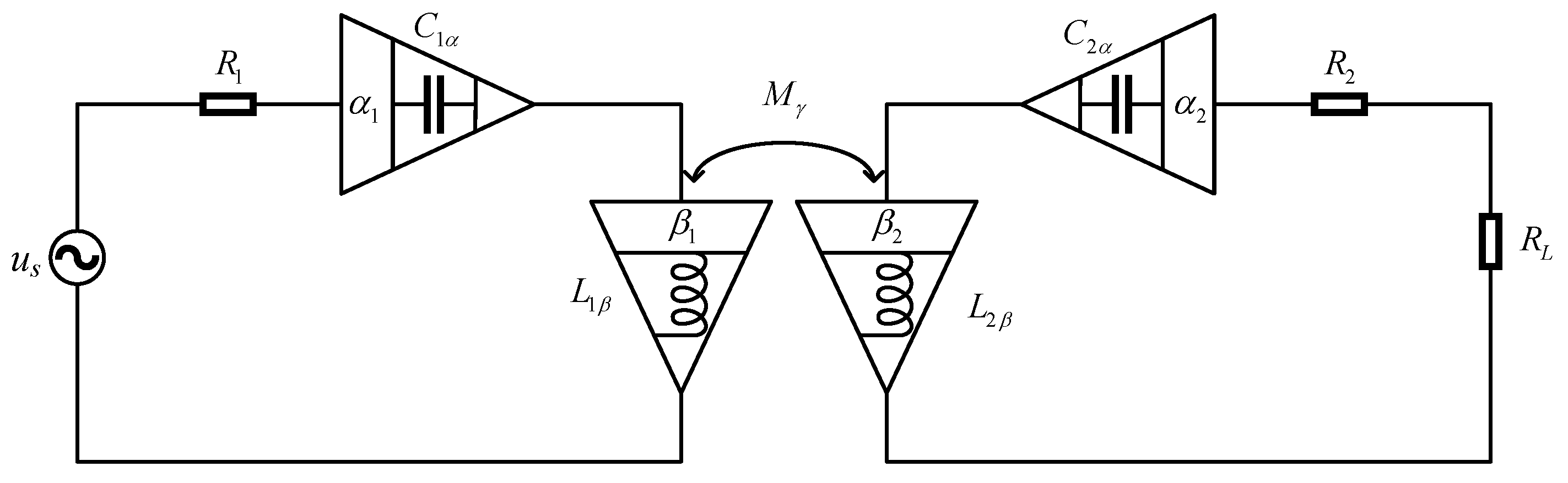
Generally, a fractional-order WPT system consists mainly of a source, transmitter, receiver, and load. The source us is usually achieved by an inverter, such as half-bridge, full-bridge, and others, which serves as power supply for the whole system. The transmitter contains an inductance L1β with fractional-order characteristics, a capacitance C1α with fractional-order characteristics, and an internal resistance R1 of the transmitting circuit. The receiver also comprises a fractional-order inductance L2β, a fractional-order capacitance C2α, an internal resistance R2 of the receiving circuit, and a load RL. The circuit coupling is realized through the mutual inductance Mγ between the transmitting and receiving coil. The simplified schematic diagram is shown in Figure 1, in which L1β and L2β are pseudo-inductance values of the fractional-order inductance of the transmitter and receiver, respectively, C1α and C2α are pseudo-capacitance values of the fractional-order capacitance of the transmitter and receiver, respectively, β1 and β2 are the fractional orders of the fractional-order inductance of the transmitter and receiver, respectively, α1 and α2 are the fractional orders of the fractional-order capacitance of the transmitter and receiver, respectively, and Mγ and γ are pseudo-inductance value and the fractional order of fractional-order mutual inductance, respectively.
The dynamics of this fractional-order WPT system can be fully described by the differential equations as follows
where i1 and i2 are currents flowing through the fractional-order inductances, uC1 and uC2 are voltages across the fractional-order capacitances, and us is the output voltage of power supply.
To simplify the analysis, give the phasor forms of Equation (3) and simplify it as
Here, Z1 is the equivalent impedance of the transmitter, Z2 is the equivalent impedance of the receiver, and ZM is the equivalent mutual impedance, which are defined as follows
where RL1 and RC1 are equivalent resistances of fractional-order inductance and fractional-order capacitance of the transmitter, respectively, XL1 and XC1 are equivalent reactances of fractional-order inductance and fractional-order capacitance of the transmitter, respectively, RL2 and RC2 are equivalent resistances of fractional-order inductance and fractional-order capacitance of the receiver, respectively, XL2 and XC2 are equivalent reactances of fractional-order inductance and fractional-order capacitance of the receiver, respectively, and RM and XM are equivalent resistance and equivalent reactance of fractional-order mutual inductance, respectively, which are described as follows
From Equations (4) and (5), the currents flowing through the fractional-order inductances of the transmitter and receiver can be derived as
Considering that the fractional-order elements have a negative resistance property, the input power Pin of the system is modified as
where sgn(x) is defined as .
The power delivered to the load Po can be expressed as
Therefore, the transmission efficiency η can be described as
When the whole system meets the condition of resonance, the angular frequencies of transmitter and receiver are equal to the angular frequency of power supply, as shown in the following
Substituting Equations (6) and (11) into Equations (8)–(10), the input power, output power, and transmission efficiency at the resonance of system are
Obviously, when the values of all fractional orders are unity, the expressions of input power, output power, and transmission efficiency are the same as those of the integer-order WPT system.
3. Analysis of Transmission Power and Efficiency
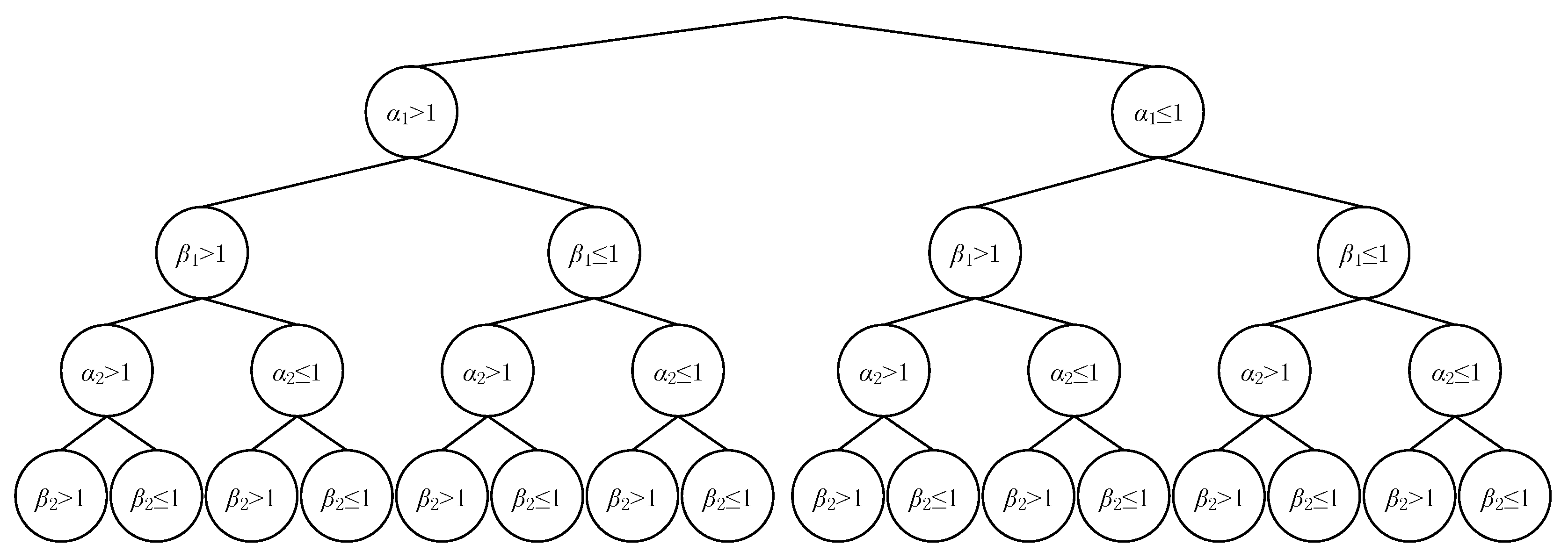
For a fractional-order element, it has a negative-resistance component when its fractional order is greater than 1. Without loss of generality, assuming the fractional order of mutual inductance is unity, that is γ = 1, for a WPT system with four fractional-order elements, there are 16 kinds of combinations of fractional orders as shown in Figure 2.
Combining the analysis of Figure 2 and Equations (8) and (10), it can be seen that the system’s input power and transmission efficiency have different expressions under different fractional orders. At present, the mechanism and manufacturing schemes of fractional-order inductors with 1 < β < 2 are still in the research stage, which is a valuable but difficult research topic; there are no articles of relevant studies. However, the fractional-order capacitors with 1 < α < 2 have been implemented in the electric power electronic devices [13]. Thus, this paper will only discuss the output power and transmission efficiency of the system with 0 < β1,2 ≤ 1 and 0 < α1,2 < 2. To intuitively show the transmission characteristics of the fractional-order WPT system, the parameters used for analysis are: the effective value of power supply Us = 20 V, internal resistances of the transmitting and receiving circuit are R1 = R2 = 0.5 Ω, pseudo-inductances values of the transmitting and receiving circuit are L1β = L2β = 100 µH, the load resistance is RL = 12 Ω, the pseudo-inductances value of mutual inductance is Mγ = 10 µH, and the resonant frequency is f0 = 300 kHz. Here, to simplify the analysis, it is assumed that the fractional-order inductances of the transmitter and receiver are identical, that is β1 = β2 = β (0 < β ≤ 1).
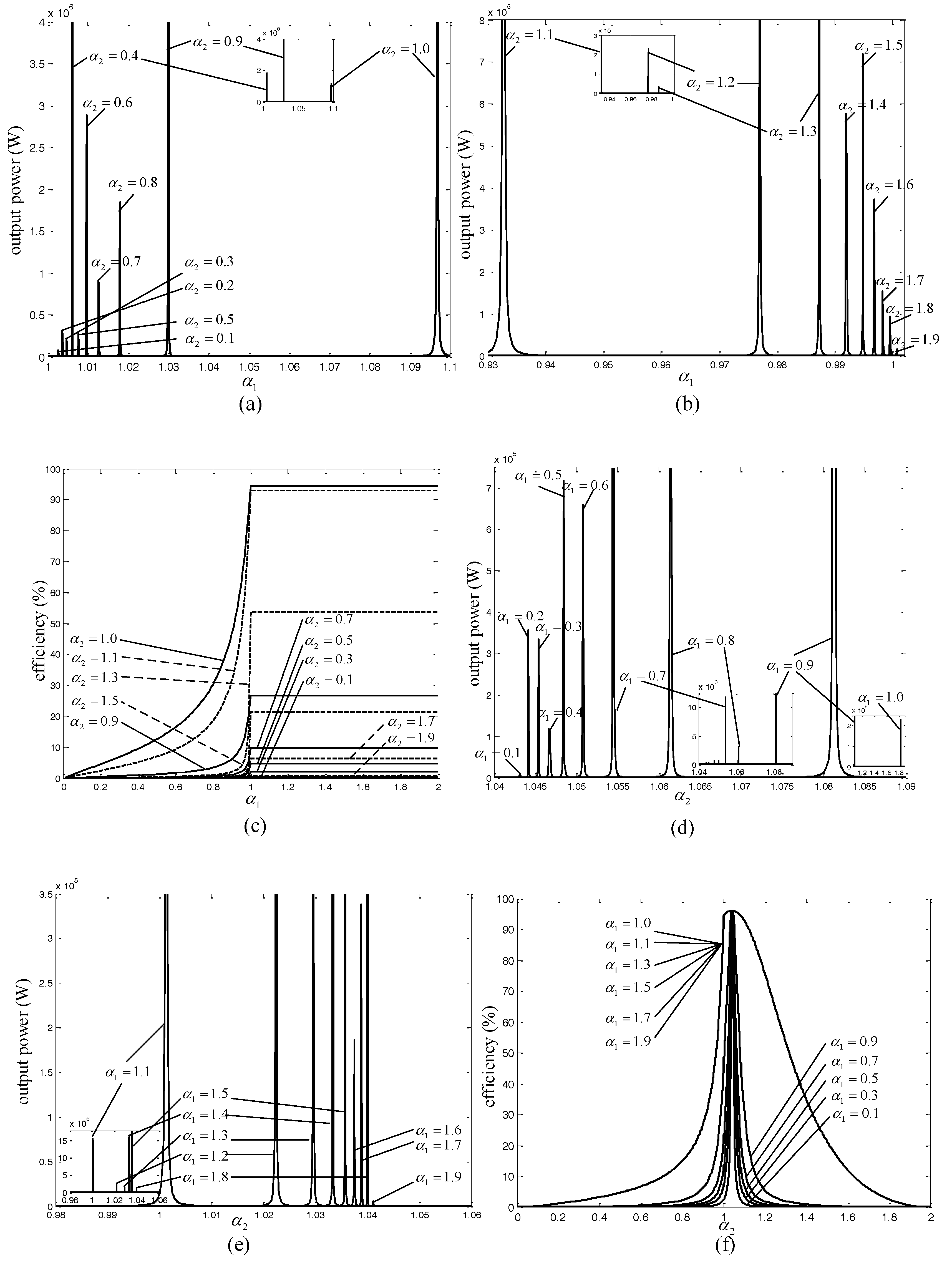
Substituting the above parameters into Equations (12)–(14), and considering the fractional order of inductance is an integer (β = 1), the curves of output power and transmission efficiency at the resonance state as a function of fractional orders (α1, α2) are very complicated, as shown in Figure 3 and Figure 4.
From Figure 3 and Figure 4, it can be seen that the variation of transmission efficiency with α1 is completely different from that with α2, but the variation of output power with α1 is very similar to that with α2. When the system is in resonance, the fractional order of the inductances is β = 1, and when the fractional order of the receiver’s resonant capacitor α2 is a fixed value, the transmission efficiency increases with the increase of α1 in the case of 0 < α1 ≤ 1, and the transmission efficiency remains constant in the case of 1 < α1 < 2. The output power has a maximum as α1 increases in the range of 0 < α1 < 2, the corresponding values of α1 are different under different fixed values of α2, but they are all close to 1 when β = 1. However, when the fractional order of the transmitter’s resonant capacitor α1 is a fixed value, the transmission efficiency increases first and then decreases with the increase of α2, which has a maximum value, and the corresponding value of α2 is close to 1. The output power also has a maximum value as α2 increases in the range of 0 < α2 < 2, the corresponding values of α2 are different under different fixed values of α1. From the above analysis, it can be seen that the system with β = 1 has better characteristics of output power and transmission efficiency when the fractional orders of transmitter’s and receiver’s resonant capacitor satisfy the conditions that 1 ≤ α1 < 2 and 0.8 < α2 < 1.2.
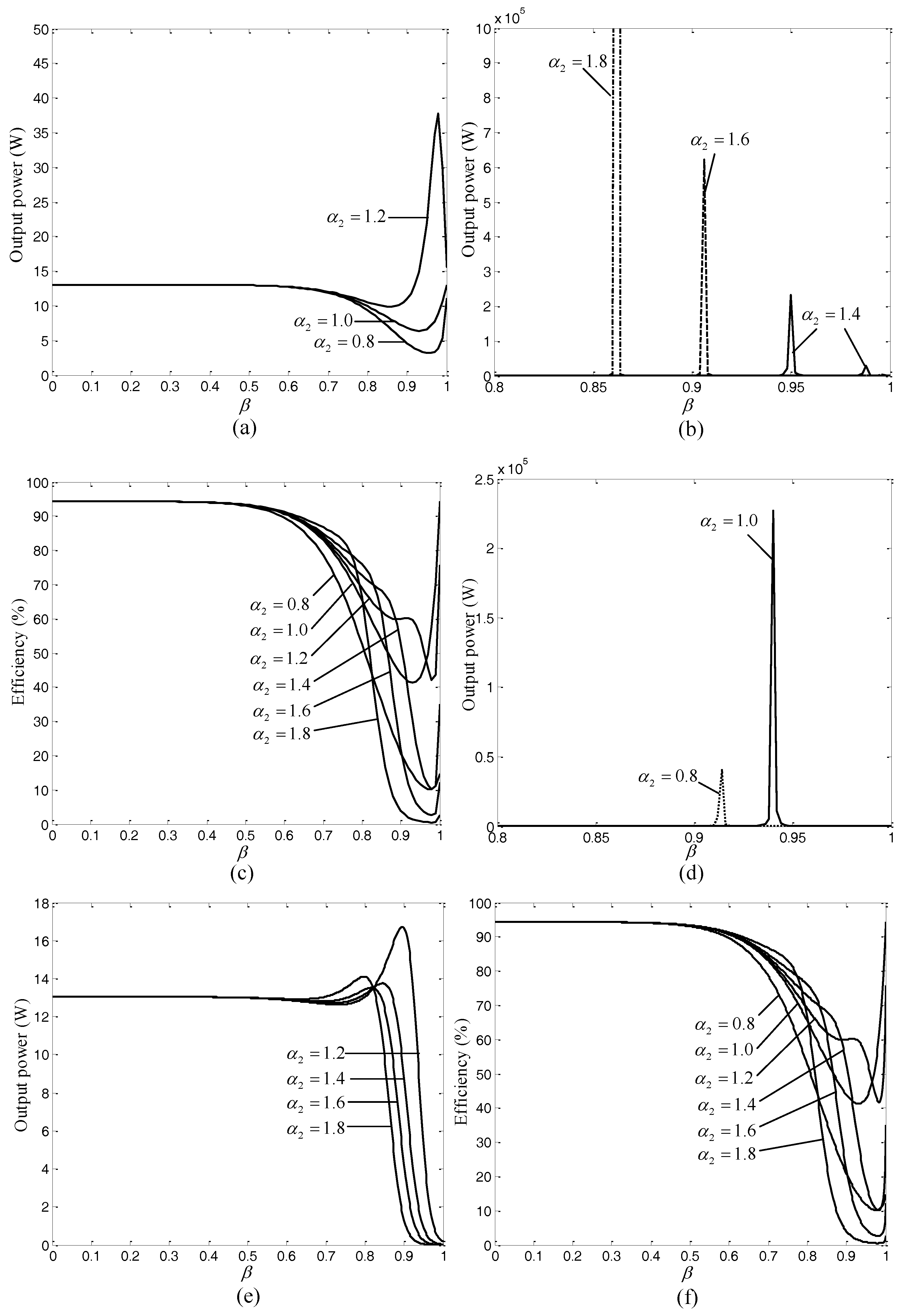
To understand the change law of output power and transmission efficiency with β, the variation of output power and transmission efficiency with β under different α1 and α2 is shown in Figure 5. As illustrated in Figure 5, the output power decreases first, then increases and then decreases with the increase of β. Whereas, the transmission efficiency decreases first and then increases with the increase of β. In addition, the law of output power varying with β is similar when α1 ≥ 1.0, and the law of transmission efficiency varying with β is not affected by the variation of α1 (1 ≤ α1 < 2), thus, only two sets of curves are given here.
4. Conclusions
This paper establishes the circuit model of the fractional-order WPT system via the phasor method, derives the modified expressions of output power and transmission efficiency, and analyzes the influence of the fractional order (α1, α2, β) on output power and transmission efficiency in detail by numerical simulation. From the theoretical analysis, it can be seen that each fractional order (α1, α2 or β) has different effects on the transmission efficiency, the transmission efficiency increases as α1 increases in the case of 0 < α1 ≤ 1, but it remains constant in the case of 1 < α1 < 2, the transmission efficiency has a maximum value with the increase of α2, and the transmission efficiency decreases first and then increases with the increase of β. Nevertheless, the effect of fractional orders (α1, α2, β) on output power is similar and the output power has a maximum value as the fractional orders (α1, α2 or β) increase. Therefore, the optimal range of fractional orders (α1, α2, β) can be determined by the above theoretical analysis, which is beneficial to obtain better characteristics of output power and transmission efficiency.
Author Contributions
X.S. established the model, analyzed the characteristics of the proposed model, implemented the simulation, and wrote this article. The project was conceived, planned and supervised by B.Z.
Acknowledgments
This project was supported by the Key Program of National Natural Science Foundation of China (Grant No. 51437005).
Conflicts of Interest
The authors declare no conflict of interest.
References
- Monje, C.A.; Chen, Y.Q.; Vinagre, B.M.; Xue, D.; Feliu, V. Fractional-Order Systems and Controls: Fundamentals and Applications; Springer: London, UK, 2010; ISBN 9781849963350. [Google Scholar]
- Miller, K.S.; Ross, B. An Introduction to the Fractional Calculus and Fractional Differential Equations; Wiley: New York, NY, USA, 1993; ISBN 9780471588849. [Google Scholar]
- Oldham, K.B.; Spanier, J. The Fractional Calculus; Academic Press: New York, NY, USA, 1974; ISBN 9780125255509. [Google Scholar]
- Podlubny, I. Fractional Differential Equations; Academic Press: New York, NY, USA, 1999; ISBN 0125588402. [Google Scholar]
- Caputo, M. Elasticità e Dissipazione; Zanichelli: Bologna, Italy, 1969. [Google Scholar]
- Lewandowski, M.; Orzyłowski, M. Fractional-order models: The case study of the supercapacitors capacitance measurement. Bull. Pol. Acad. Sci. Tech. Sci. 2017, 65, 449–457. [Google Scholar] [CrossRef]
- Machado, M.A.T.; Galhano, A.M.S.F. Fractional order inductive phenomena based on the skin effect. Nonlinear Dyn. 2012, 68, 107–115. [Google Scholar] [CrossRef]
- Cisse, H.T.; Ablart, G.; Camps, T.; Olivie, F. Influence of the electrical parameters on the input impedence of a fractal structure realised on silicon. Chaos Solitons Fractals 2005, 24, 479–490. [Google Scholar] [CrossRef]
- Radwan, A.G. Stability analysis of the fractional-order RLβCα circuit. J. Fract. Calculus Appl. 2012, 3, 1–15. [Google Scholar]
- Radwan, A.G.; Salama, K.N. Fractional-order RC and RL circuits. Circuits Syst. Signal Process. 2012, 31, 1901–1915. [Google Scholar] [CrossRef]
- Soltan, A.; Radwan, A.G.; Soliman, A.M. Fractional-order mutual inductance: Analysis and design. Int. J. Circuit Theory Appl. 2016, 44, 85–97. [Google Scholar] [CrossRef]
- Kurs, A.; Karalis, A.; Moffatt, R.; Joannopolos, J.D.; Fisher, P.; Soljačić, M. Wireless power transfer via strongly coupled magnetic resonances. Science 2007, 317, 83–86. [Google Scholar] [CrossRef] [PubMed]
- Jiang, Y.; Zhang, B. High-power fractional-order capacitor with 1 < α < 2 based on power converter. IEEE Trans. Ind. Electron. 2018, 65, 3157–3164. [Google Scholar] [CrossRef]
Figure 1.
Simplified schematic of the fractional-order wireless power transmission (WPT) system.

Figure 2.
Tree diagram of combinations of fractional orders.

Figure 3.
Theoretical curves of output power and transmission efficiency as a function of fractional order (α1, α2) when β = 1: (a) Output power versus α1 when 0 < α2 ≤ 1 and β = 1; (b) Output power versus α1 when 1 < α2 < 2 and β = 1; (c) Transmission efficiency versus α1 when 0 < α2 < 2 and β = 1; (d) Output power versus α2 when 0 < α1 ≤ 1 and β = 1; (e) Output power versus α2 when 1 < α1 < 2 and β = 1; (f) Transmission efficiency versus α2 when 0 < α1 < 2 and β = 1.

Figure 4.
Three-dimensional (3-D) demonstration of input power, output power, and transmission efficiency versus fractional order (α1, α2) when β = 1: (a) Input power versus α1 and α2 when β = 1; (b) Output power versus α1 and α2 when β = 1; (c) Transmission efficiency versus α1 and α2 when β = 1.
Figure 4.
Three-dimensional (3-D) demonstration of input power, output power, and transmission efficiency versus fractional order (α1, α2) when β = 1: (a) Input power versus α1 and α2 when β = 1; (b) Output power versus α1 and α2 when β = 1; (c) Transmission efficiency versus α1 and α2 when β = 1.
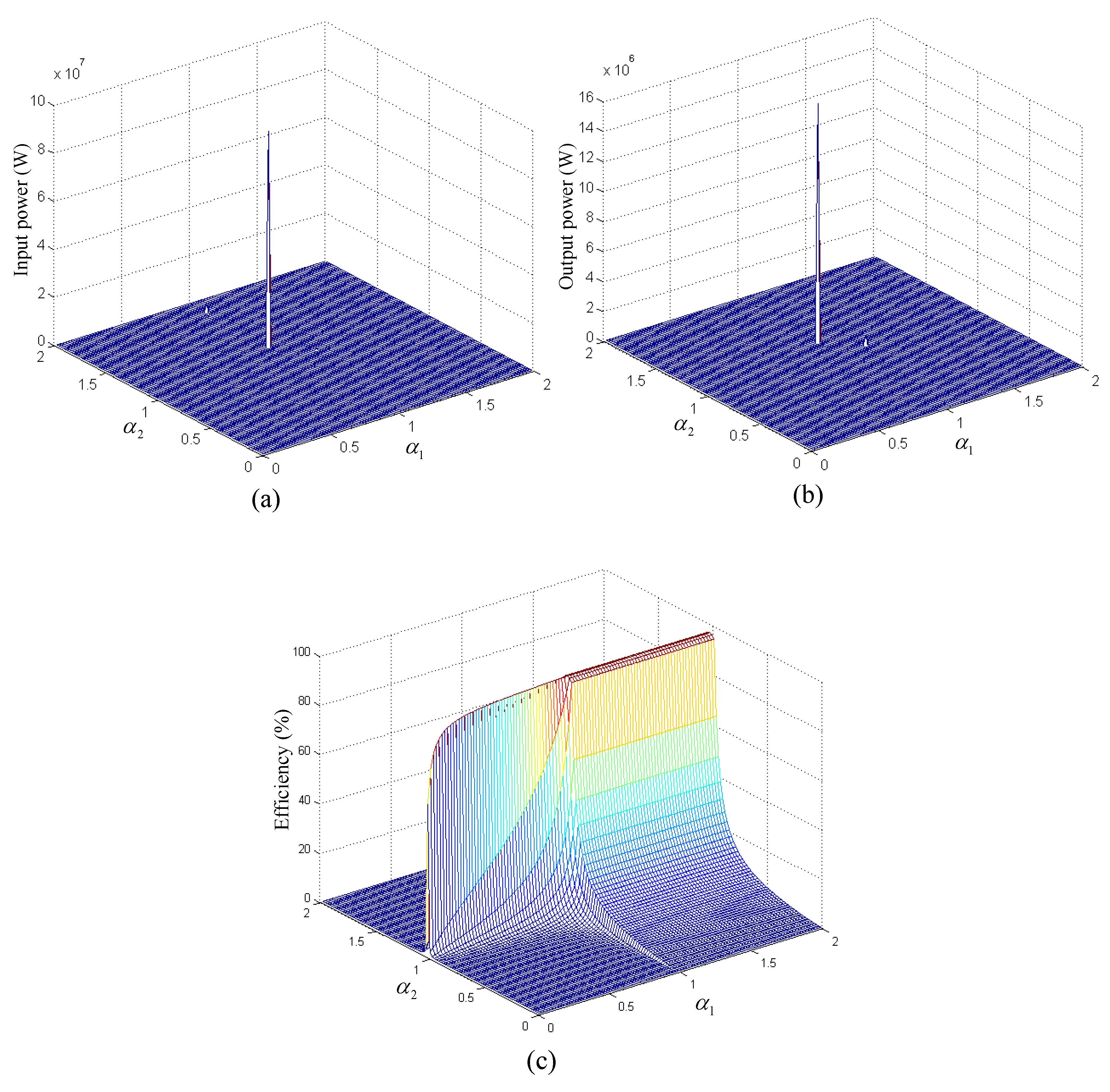
Figure 5.
Theoretical curves of output power and transmission efficiency as a function of fractional order β when 1 ≤ α1 < 2 and 0.8 ≤ α2 < 2: (a) Output power versus β when α1 = 1.0 and 0.8 ≤ α2 ≤ 1.2; (b) Output power versus β when α1 = 1.0 and 1.4 ≤ α2 < 2; (c) Transmission efficiency versus β when α1 = 1.0 and 0.8 ≤ α2 < 2; (d) Output power versus β when α1 = 1.2 and 0.8 ≤ α2 ≤ 1.2; (e) Output power versus β when α1 = 1.2 and 1.2 ≤ α2 < 2; (f) Transmission efficiency versus β when α1 = 1.2 and 0.8 ≤ α2 < 2.

© 2018 by the authors. Licensee MDPI, Basel, Switzerland. This article is an open access article distributed under the terms and conditions of the Creative Commons Attribution (CC BY) license (http://creativecommons.org/licenses/by/4.0/).
Share and Cite
MDPI and ACS Style
Shu, X.; Zhang, B. The Effect of Fractional Orders on the Transmission Power and Efficiency of Fractional-Order Wireless Power Transmission System. Energies 2018, 11, 1774. https://doi.org/10.3390/en11071774
AMA Style
Shu X, Zhang B. The Effect of Fractional Orders on the Transmission Power and Efficiency of Fractional-Order Wireless Power Transmission System. Energies. 2018; 11(7):1774. https://doi.org/10.3390/en11071774
Chicago/Turabian StyleShu, Xujian, and Bo Zhang. 2018. "The Effect of Fractional Orders on the Transmission Power and Efficiency of Fractional-Order Wireless Power Transmission System" Energies 11, no. 7: 1774. https://doi.org/10.3390/en11071774
Note that from the first issue of 2016, this journal uses article numbers instead of page numbers. See further details here.