Analysis, Design and Implementation of Droop-Controlled Parallel-Inverters Using Dynamic Phasor Model and SOGI-FLL in Microgrid Applications

Abstract

The droop control strategy is widely used in islanded microgrids to control power flows according to the load condition, with the absence of a critical communication line, interfacing distributed energy sources to provide for the active and reactive power demand of loads. In this case, the system modeling for both steady-state and transient time is one of the key issues of a droop-controlled system for an inverter-based microgrid (MG). With the rapid development of microgrids, it is essential to identify the system stability and optimize the control parameters, taking into account the network and control dynamics caused by multiple tasks such as electric signal filtering, network synchronization, and so on. Therefore, in order to improve model accuracy and determine control coefficients, this paper analyzes and extends a dynamic phasor-based model to the droop-controlled parallel-inverters, considering network and control dynamics such as a low-pass filter, a second-order generalized integrator frequency-locked-loop (SOGI-FLL), and a system operating sequence. Moreover, discussed in this paper are both the design approaches for and the implementation of a droop-controlled parallel-inverter, which enables the system to be stable and reliable. To demonstrate the effectiveness and validity of this paper, PSIM simulation was performed and two parallel-inverters were combined as the proposed design procedure for the 4-kVA prototypes.

1. Introduction

Recently, the energy crisis and environmental pollution have become increasingly serious. Distributed generation (DG) has come into the spotlight in meeting future energy demands [1]. A cluster of DG units such as a photovoltaic system, wind turbines, an energy storage system, and local loads constitute a microgrid, which can be operated in either grid-connected or islanded modes. The operation of a microgrid is defined in the IEEE std. 1547.4-2011, and this paper is mainly focused on the islanded mode operation.

The interfaces between the DG and the microgrid are generally based on power electronic devices acting as voltage sources, especially a voltage-source-inverter (VSI) in a microgrid [2,3]. In the case of microgrids, these power electronic devices are connected in parallel to the microgrid.

In order to control the power flow in an inverter-based islanded microgrid without any communication lines, the droop control scheme has been widely used [2]. Conventionally, the coefficients of a droop curve are designed considering the maximum power rating and maximum possible error of voltage amplitude and frequency [4,5]. However, using the designed coefficients according to the conventional droop control, the power sharing and control performance between modules are not excellent because there are inherent limitations with a conventional droop control scheme where parallel-inverters should have same per-unit impedance in which share the load power accurately [6]. The conventional droop control presents other drawbacks, and much research has been performed to improve the performance of the conventional droop control. One of the most significant contributions of these studies is the virtual impedance to match output impedances of each inverter equally to improve power sharing [7,8]. Using virtual impedance, power sharing can be achieved uniformly, but the voltage and frequency drop increases if the secondary control is not applied in the droop control, and other research has been performed to solve this problem [9,10,11].

Meanwhile, the dynamic stability of an inverter-based microgrid has been highlighted for many years. For AC microgrids, single-phase inverters not only inject micro-sources generated from DGs into the grid, but also perform additional operations such as power conditioning and grid synchronization [12]. As these power systems become enlarged, it is essential to identify the system stability and optimize the control parameters. Compared to the conventional power system, a microgrid is more inclined to unbalanced and harmonic operating conditions due to intermittent energy sources and the penetrations of power electronic devices. In this case, dealing with stability issues, it is significant to model microgrids with DGs such as wind and Photovoltaic (PV) with power electronic converters [13].

In modeling microgrids, transforming the system models to a synchronous rotating (d-q) frame is the universal technique. One of the advantages in analyzing the inverter system in a synchronous rotating frame is that steady-state operator quantities have constant values under balanced conditions [14]. However, if there are unbalanced conditions such as the system or other harmonics, the three-phase current becomes unbalanced and contains all three sequence components. From the viewpoint of simulation performance, it implies that the step size of the simulation should be small enough to capture the oscillations with maximum frequency, which makes the simulation inefficient during unbalanced conditions [15].

Thus, a modeling technique using dynamic phasors has been used to model and simulate a switch-mode power conversion system [16,17,18]. Hence, the dynamic phasor-based model, for both a steady and transient state, is introduced to provide robust dynamical simulation in order to support the design of coordinated protection schemes and operational control algorithms [12]. In Reference [12], a model of a dynamic, phasors-based, single-phase inverter is analyzed and modeled through three sections: a boost stage, a DC-to-AC inverter stage, and a filtering stage. The study demonstrates the simulation of dynamic phasor models, considering harmonics are faster than a detailed model of the inverter, but it does not include the control structure such as the droop control. In Reference [19], dynamic phasor-based modeling and stability analysis of a droop-controlled inverter were performed to predict the stability margins of the system. As a result, the design of control and power stage parameters were realized based on a dynamic phasor model, but it is limited to a droop control structure, such as droop coefficients and a low pass filter, which is used for power calculation.

In this paper, a design method of droop-controlled single-phase parallel-inverters is discussed based on a dynamic phasor approach in microgrid applications. The droop control structure is analyzed and modeled using a dynamic phasor, and it is utilized for the determination of the dynamic stability of the power controller. In order to determine the control parameters, the inverter modeling and voltage/current controller design are performed based on a synchronous rotating frame, as usual. In addition, a second-order generalized integrator frequency-locked-loop (SOGI-FLL) is applied to minimize the inherent tradeoff in inverter-based droop-controlled islanded microgrid applications, and it is considered for the implementation of droop-controlled parallel-inverters in this paper. Furthermore, a control sequence of operation is also presented to implement the actual operation of the droop control-based parallel operation of single-phase inverters. As a result, this paper contributes to the design of droop-controlled parallel-inverters by considering the design factors required for the implementation of parallel-inverters, such as stability analysis, digital filtering, the control sequence for network synchronization, and so on. To demonstrate the validity of this paper, PSIM simulation was performed, and two parallel-inverters are implemented in accordance with the proposed design procedure for the 4-kVA prototypes.

2. Dynamics of Power Delivery in Parallel-Inverters

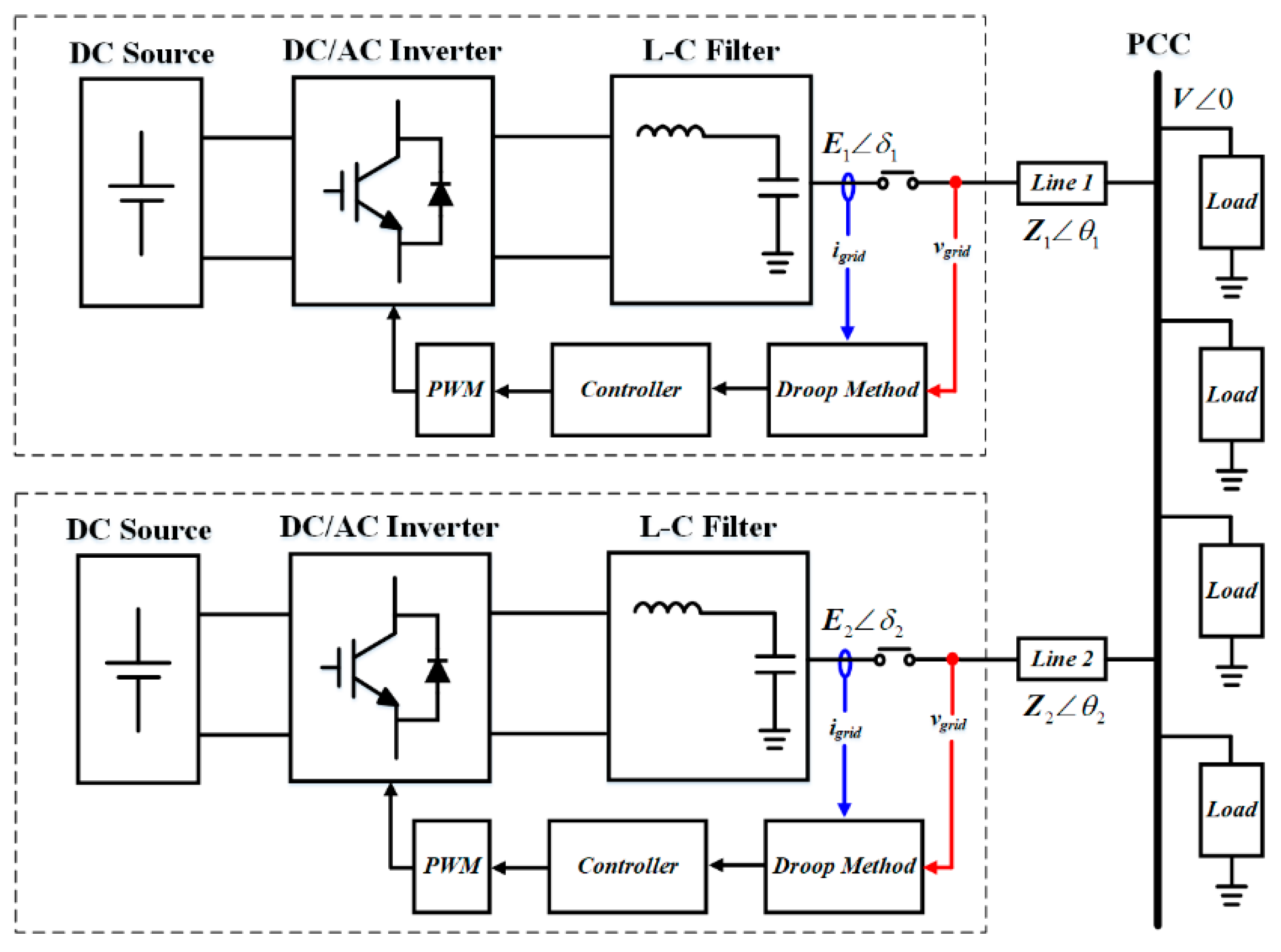
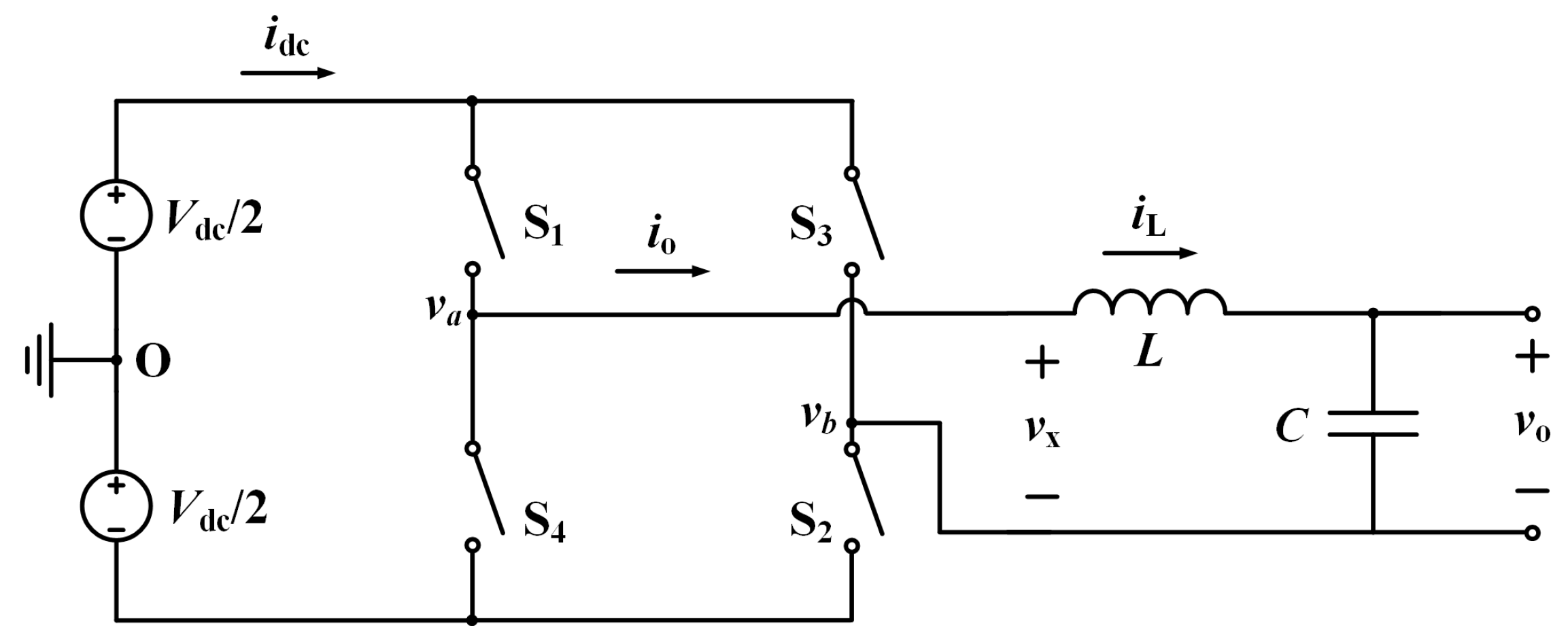
2.1. System Configuration

Figure 1 shows the schematic diagram of droop-controlled parallel inverters for MG applications, which includes the DC power source, L-C filter, and DC/AC inverters. DC/AC inverters supply for local loads by regulating the voltage/frequency of its output, and this enables the parallel-inverters to achieve proportional load sharing. In Figure 1, E_i and δ_i are peak voltage and the power angle difference of i-th inverter output, respectively, Z_i and θ_i are magnitude and phase of the i-th line impedance, respectively, and V is the AC bus voltage.

2.2. Dynamics of Power Delivery

Generally, the droop control is a method of controlling active and reactive power using the phase and magnitude of the voltage output from the inverter. Therefore, the droop equations can be derived by the following procedure.

First of all, by using the complex power equation, the inverter output active and reactive power, based on the AC bus voltage, can be expressed according to Figure 1 as follows in Equation (1).

$$S=V\cdot I^{*}=V\angle 0\cdot {\left(\frac{E\angle \delta -V\angle 0}{Z\angle \theta }\right)}^{*}$$

(1)

Thus, the active and reactive power can be simplified as follows in Equation (2). R and X are the resistive and inductive components of the line impedance.

$$\left[\begin{array}{l}P\\ Q\end{array}\right]=\frac{V}{R^2+X^2}\left[\begin{array}{ccc}\begin{array}{l}ER\\ EX\end{array}& \begin{array}{l}EX\\ -ER\end{array}& \begin{array}{l}-RV\\ -VX\end{array}\end{array}\right]\left[\begin{array}{c}\cos \delta \\ \sin \delta \\ 1\end{array}\right]$$

(2)

To obtain the characteristic between P, Q, and E, δ, partial differentiation is used for the sensitivity analysis as follows:

$$\left[\begin{array}{l}\frac{\partial P}{\partial \delta }\\ \frac{\partial Q}{\partial \delta }\end{array}\right]=-\frac{EV}{R^2+X^2}\left[\begin{array}{cc}R& -X\\ X& R\end{array}\right]\left[\begin{array}{c}\sin \delta \\ \cos \delta \end{array}\right]$$

(3)

$$\left[\begin{array}{l}\frac{\partial P}{\partial E}\\ \frac{\partial Q}{\partial E}\end{array}\right]=\frac{V}{R^2+X^2}\left[\begin{array}{cc}R& X\\ X& -R\end{array}\right]\left[\begin{array}{c}\cos \delta \\ \sin \delta \end{array}\right]$$

(4)

Usually, droop control is based on the important assumption that when the inverter output and the ac bus are well synchronized, the phase difference will be very small ($\delta \approx 0$). Additionally, the inverter will output the same magnitude of voltage as the AC bus. Thus, the following assumption can be obtained:

$$\sin \delta \approx 0, \cos \delta \approx 1$$

(5)

$$E=V$$

(6)

Thus, Equations (3) and (4) can be simplified as follows

$$\frac{\partial P}{\partial \delta }=-\frac{V^2\cdot X}{R^2+X^2}=K_{P\delta }$$

(7)

$$\frac{\partial Q}{\partial \delta }=-\frac{V^2\cdot R}{R^2+X^2}=K_{Q\delta }$$

(8)

$$\frac{\partial P}{\partial E}=\frac{V\cdot R}{R^2+X^2}=K_{PE}$$

(9)

$$\frac{\partial Q}{\partial E}=\frac{V\cdot X}{R^2+X^2}=K_{QE}$$

(10)

Using the Equations (7)–(10), depending on whether the dominant component of the line impedance is inductive or resistive, the variables influencing the active and the reactive power are different. As shown in

Table 1. Droop characteristics according to the dominant component of line impedance.

Parameter	Pure Inductive (R = 0)	Pure Resistive (X = 0)
$K_{P\delta }$	$\frac{V^2}{X}$	0
$K_{PE}$	0	$\frac{V}{R}$
$K_{Q\delta }$	0	$-\frac{V^2}{R}$
$K_{QE}$	$\frac{V}{X}$	0

, when the dominant component of line impedance is inductive, the active and reactive power are influenced by phase difference and inverter output voltage, respectively. When it is resistive, the active and reactive power are influenced by inverter output voltage and phase difference, respectively.

Usually, the inverter output impedance is mostly inductive in parallel inverters because the filter inductance is large enough to ignore the resistive component. In order for parallel inverters to share the load, the inductive droop equations are derived as follows:

$$\Delta \omega ={\omega }^{*}-K_P\cdot \Delta P+K_P\cdot P^{*}$$

(11)

$$\Delta E=E^{*}-K_Q\cdot \Delta Q+K_Q\cdot Q^{*}$$

(12)

In this case, droop coefficients K_P and K_Q restrict the range of $\Delta \omega$ and $\Delta E$, respectively, and the increase of droop coefficients improves the dynamics, but it also enlarges the error range in terms of $\Delta \omega$ and $\Delta E$ under all load conditions, as shown in Figure 2. Therefore, in order to achieve both the same load sharing and high dynamic response in inverter-based MG applications, the tradeoff between dynamic characteristics and steady-state error should be reduced.

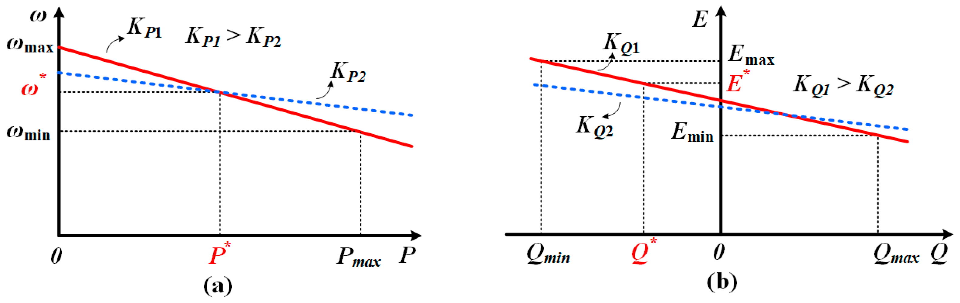
2.3. Dynamics of Droop Control

Small signal modeling is well known as a very accurate system modeling strategy, and studies have long been conducted. It considers the variation of the output value with respect to the change of the input value. It is necessary to know the variation amount of active power, the reactive power according to the variation amount of the phase difference, and the output voltage of the inverter, which are obtained in Equations (7)–(10). In this section, the general procedure for performing a small-signal model of the system is carried out using the equations mentioned previously.

The variation of inverter output active and reactive power can be expressed as Equation (13), using coefficients K_PE, K_Pδ, K_QE, and K_Qϕ.

$$\left[\begin{array}{c}\Delta P\\ \Delta Q\end{array}\right]=\left[\begin{array}{cc}{K}_{PE}& K_{P\delta }\\ K_{QE}& K_{Q\delta }\end{array}\right]\left[\begin{array}{c}\Delta E\\ \Delta \delta \end{array}\right]$$

(13)

From droop Equations (11) and (12), the variation of the frequency and the inverter output voltage are directly affected by the instantaneous active and reactive power rather than the command active and reactive power, which are a constant value. Accordingly, Equations (11) and (12) can be simplified as follows in Equations (14) and (15):

$$\Delta \omega =-K_P\cdot \Delta P$$

(14)

$$\Delta E=-K_Q\cdot \Delta Q$$

(15)

Additionally, as shown in Equation (16), time-varying active and reactive power are averaged to change them as a constant value by using a second-order low-pass filter, whose characteristics are different according to the cutoff frequency ω_f and the damping ratio ζ.

$$\left[\begin{array}{c}\Delta \omega \\ \Delta E\end{array}\right]=-\frac{{\omega }_f{}^2}{s^2+2\zeta {\omega }_{f}s+{\omega }_f{}^2}\left[\begin{array}{cc}{K}_P\cdot K_{PE}& K_P\cdot K_{P\delta }\\ K_Q\cdot K_{QE}& K_Q\cdot K_{Q\delta }\end{array}\right]\left[\begin{array}{c}\Delta E\\ \Delta \delta \end{array}\right]$$

(16)

Finally, by integrating the above-mentioned equations, the characteristic equation for small signal modeling based droop control inverters is derived as Equations (17) and (18).

$$a{s}^5+b{s}^4+c{s}^3+d{s}^2+es+f=0$$

(17)

$$\begin{array}{l}a=1\\ b=4\zeta {\omega }_f\\ c=(2+K_Q{K}_{QE}+4{\zeta }^2){\omega }_f{}^2\\ d=\{(4+2K_Q{K}_{QE})\zeta {\omega }_f+K_P{K}_{P\delta }\}{\omega }_f{}^2\\ e=\{(1+K_Q{K}_{QE}){\omega }_f+2K_P{K}_{P\delta }\zeta \}{\omega }_f{}^3\\ f=(K_P{K}_{P\delta }+K_P{K}_{P\delta }{K}_Q{K}_{QE}-K_P{K}_{PE}{K}_Q{K}_{Q\delta }){\omega }_f{}^4\end{array}$$

(18)

The coefficients of the characteristic equation determine the system transient response and stability. Therefore, it is necessary to analyze the stability of the system according to the change of the coefficients because the criterion on how to select the coefficient is very important. As shown in Equation (18), the position of the pole changes with the variation of the cutoff frequency and droop coefficients, and the system stability can be determined by its position in left-half-plane (LHP) or right-half-plane (RHP). The position of the pole is in a stable region when it is in the LHP, and it can be used as an indicator in selecting the appropriate coefficient.

3. Modeling and Analysis of Dynamic Phasor-Based Droop-Controlled Inverter

3.1. Dynamic Phasor-Based Modeling

Dynamic phasors were introduced as a way of improving the bandwidth of transient simulation to include the dynamics of power equipment such as power electronics converter [17]. A random function can be expressed as a sum of complex phasors by using the dynamic phasor. It is derived from the Fourier series, which means that periodic functions can be represented by the sum of harmonics, so it has a very similar form. As shown in

Table 2. General formula of Fourier series and dynamic phasor.

Category	General Formula	k-th Coefficient
Fourier Series	$X(t)={\displaystyle \sum _{k=-\infty }^{\infty }{X}_k\cdot e^{jk{\omega }_s\tau }}$	$X_k=\frac{1}{T}{\displaystyle {\int }_0^{T}X(t)\cdot e^{-jk{\omega }_s\tau }}d\tau$
Dynamic Phasor	$X(t)={\displaystyle \sum _{k=-\infty }^{\infty }{X}_k(t)\cdot e^{jk{\omega }_s\tau }}$	$X_k(t)={\langle X\rangle }_k=\frac{1}{T}{\displaystyle {\int }_0^{T}X(t)\cdot e^{-jk{\omega }_s\tau }}d\tau$

, the significant difference between the Fourier series and a dynamic phasor is that the k-th dynamic phasor coefficient X_k(t) is time-varying. It overcomes the shortage for the application of time-invariant systems, such as the Fourier transform, Laplace transform, and so on.

Additionally, the parasitic components of the inductor and capacitor were considered by using a dynamic phasor. This can be seen through the following equation, which is derived from the general dynamic phasor formula.

$${\langle \frac{dx}{dt}\rangle }_k=\frac{d}{dt}{\langle x\rangle }_k+jk{\omega }_s\cdot {\langle x\rangle }_k$$

(19)

As shown in Equation (19), there is a complex term that varies according to k, and it can be considered as a parasitic component. For example, a dynamic phasor can be applied to the voltage equation of an inductor, shown in Equation (20), as follows in Equation (21), where v_L, i_L represent voltage and current of inductor respectively.

$$v_L=L\cdot \frac{d{i}_L}{dt}$$

(20)

$$\begin{array}{c}{\langle v_L\rangle }_k=L\frac{d}{dt}{\langle i_L\rangle }_k+jk{\omega }_{s}L\cdot {\langle i_L\rangle }_k\\ {\langle v_L\rangle }_0=L\frac{d}{dt}{\langle i_L\rangle }_0+0\\ {\langle v_L\rangle }_1=L\frac{d}{dt}{\langle i_L\rangle }_1+j{\omega }_{s}L\cdot {\langle i_L\rangle }_1\\ ⋮\end{array}$$

(21)

From Equation (21), it can be confirmed that the complex term is generated according to k, which is regarded as a parasitic component. Consequently, the use of a dynamic phasor reveals that an inductor has a parasitic component in series and a capacitor has one in parallel.

Therefore, the coefficients are changed by application to Equations (7)–(10) in consideration of the additional parasitic component generated by the dynamic phasor and expressed as follows:

$$K_{PE}{}^{\prime }=\frac{V(R+sL)}{{(R+sL)}^2+{(\omega L)}^2}$$

(22)

$$K_{P\delta }{}^{\prime }=\frac{V^2(\omega L)}{{(R+sL)}^2+{(\omega L)}^2}$$

(23)

$$K_{QE}{}^{\prime }=\frac{V(\omega L)}{{(R+sL)}^2+{(\omega L)}^2}$$

(24)

$$K_{Q\delta }{}^{\prime }=-\frac{V^2(R+sL)}{{(R+sL)}^2+{(\omega L)}^2}$$

(25)

Equations (22)–(25) can be replaced instead of K_PE, K_Pδ, K_QE, and K_Qδ which are in the variation of active and reactive power of Equation (13), as follows in Equation (26):

$$\left[\begin{array}{c}\Delta P\\ \Delta Q\end{array}\right]=\left[\begin{array}{cc}{K}_{PE}{}^{\prime }& K_{P\delta }{}^{\prime }\\ K_{QE}{}^{\prime }& K_{Q\delta }{}^{\prime }\end{array}\right]\left[\begin{array}{c}\Delta E\\ \Delta \delta \end{array}\right]$$

(26)

With the same procedure as in Section 2.2, by using Equations (14) and (15) and a second-order low-pass filter, the following simplification can be made, and its closed loop model is expressed. Detailed description will be omitted from this section because it was handled in Section 2.2.

$$\left[\begin{array}{c}\Delta \omega \\ \Delta E\end{array}\right]=-\frac{{\omega }_f{}^2}{s^2+2\zeta {\omega }_{f}s+{\omega }_f{}^2}\left[\begin{array}{cc}{K}_P\cdot K_{PE}{}^{\prime }& K_P\cdot K_{P\delta }{}^{\prime }\\ K_Q\cdot K_{QE}{}^{\prime }& K_Q\cdot K_{Q\delta }{}^{\prime }\end{array}\right]\left[\begin{array}{c}\Delta E\\ \Delta \delta \end{array}\right]$$

(27)

As a result, the characteristic Equations (28) and (29) for dynamic phasor modeling of droop-controlled inverters are derived.

$$a^{\prime }{s}^7+b^{\prime }{s}^6+c^{\prime }{s}^5+d^{\prime }{s}^4+e^{\prime }{s}^3+f^{\prime }{s}^2+g^{\prime }s+h^{\prime }=0$$

(28)

$$\begin{array}{l}{a}^{\prime }=L^2\\ b^{\prime }=2RL+4\zeta {\omega }_f{L}^2\\ c^{\prime }=R^2+{\omega }^2{L}^2+8\zeta {\omega }_{f}RL+2{\omega }_f{}^2{L}^2+4{\zeta }^2{\omega }_f{}^2{L}^2\\ d^{\prime }=4{\omega }_f(\zeta R^2+\zeta {\omega }^2{L}^2+R{\omega }_{f}L+2{\zeta }^{2}R{\omega }_{f}L+\zeta {\omega }_f{}^2{L}^2)\\ e^{\prime }=(2R^2+2{\omega }^2{L}^2+K_Q{V}_{dc}\omega L+4{\zeta }^2{R}^2+4{\zeta }^2{\omega }^2{L}^2+8\zeta RL{\omega }_f+{\omega }_f{}^2{L}^2){\omega }_f{}^2\\ f^{\prime }=(4\zeta R^2{\omega }_f+4\zeta {\omega }^2{L}^2{\omega }_f+2\zeta K_Q{V}_{dc}\omega L{\omega }_f+K_P{V}_{dc}{}^2\omega L+2RL{\omega }_f){\omega }_f{}^2\\ g^{\prime }=(R^2{\omega }_f+{\omega }^2{L}^2{\omega }_f+K_Q{V}_{dc}\omega L{\omega }_f+2\zeta K_P{V}_{dc}{}^2\omega L){\omega }_f{}^3\\ h^{\prime }=(\omega L+K_Q{V}_{dc})V_{dc}{}^2{K}_P{\omega }_f{}^4\end{array}$$

(29)

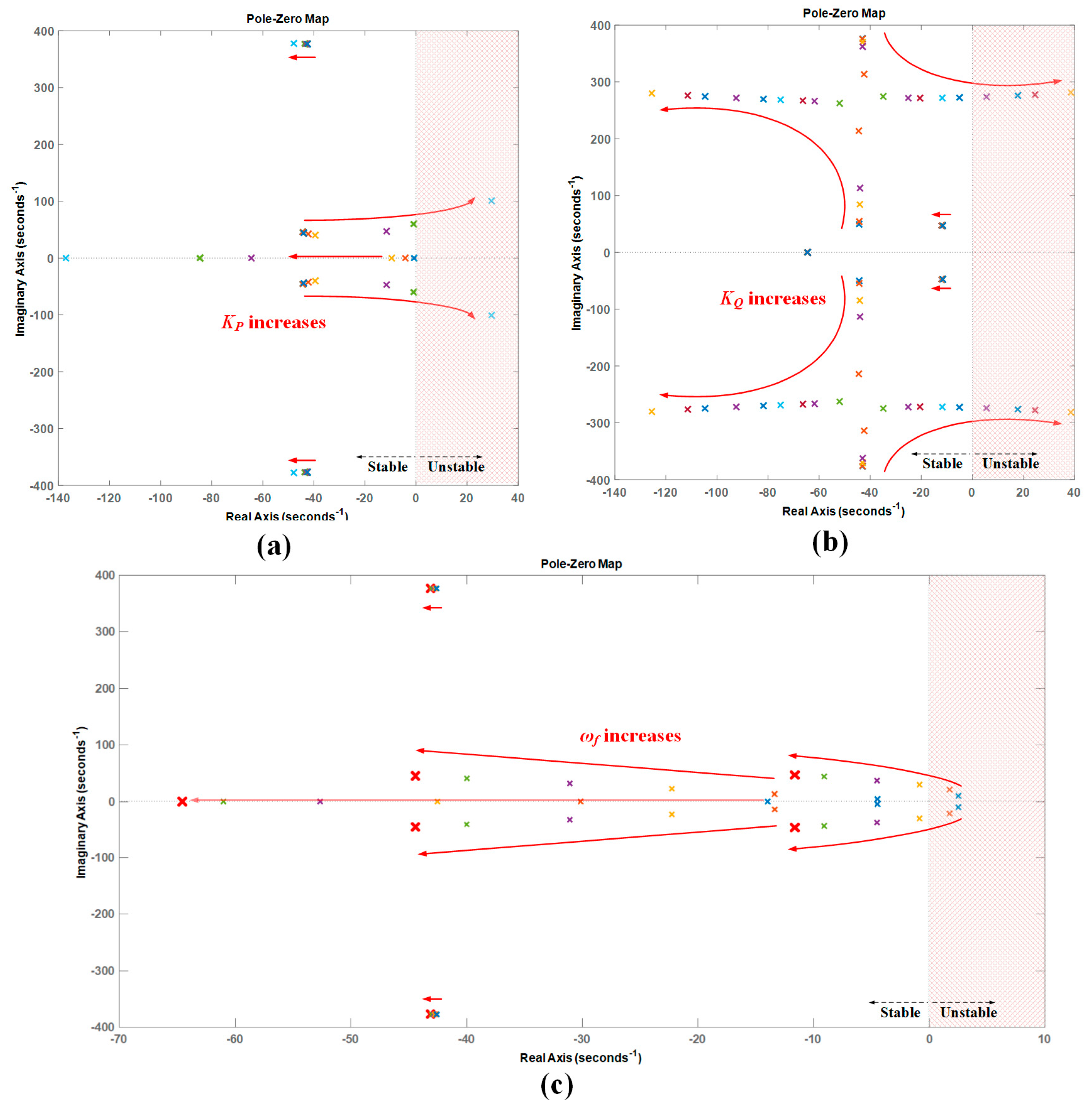
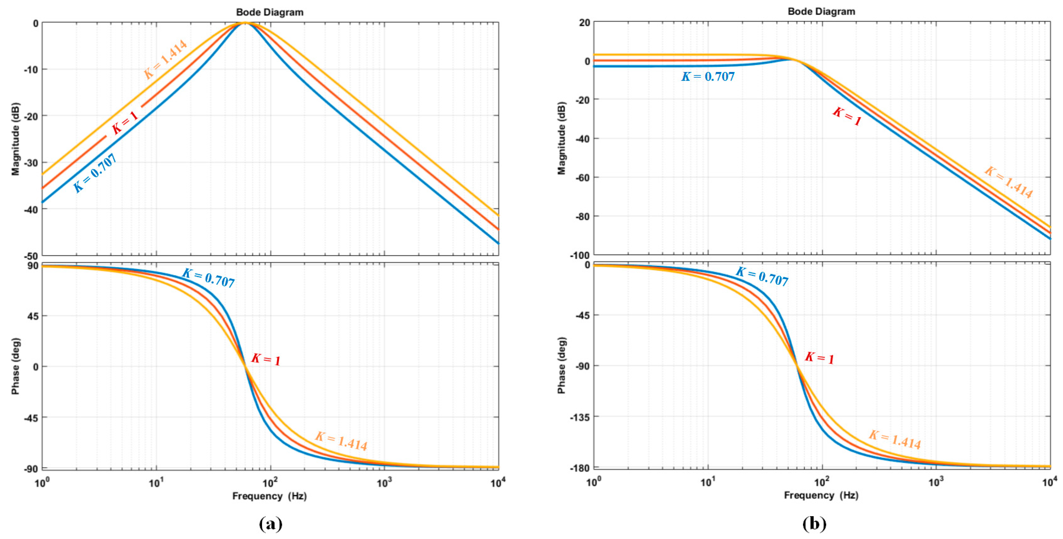
3.2. Stability Analysis and Selection of Droop Coefficients

The system transient response and stability are determined by coefficients of the characteristic equation, so determination of the droop coefficients, damping ratio, and cutoff frequency is important to obtain good performance. Accordingly, MATLAB (R2015a) simulation for analyzing the characteristic equation is implemented by using the system shown in Figure 3, which demonstrates the configuration of the droop-controlled inverters based on dynamic phaosr model. This figure represents the stability determination by using the pole zero map of Equations (28) and (29). The stability can be defined by how much of the cutoff frequency and the droop coefficients are selected. Depending on the characteristics of the droop control, proper coefficients should be selected considering the dynamic characteristics and steady-state error. The fixed values of the system parameters used in this stability analysis are listed in

Table 3. Simulation and experimental parameters.

Parameters	Value [Unit]	Parameters	Value [Unit]
Maximum Power Rating P	4 kW/a module	Reference P	1.9 kW
Maximum Power Rating Q	1 kVar/a module	Reference Q	0
DC voltage	350 Vdc	Droop coefficient KP	0.0005
AC Output voltage	220 Vrms	Droop coefficient KQ	0.0001
AC Output frequency	60 Hz	Line impedance R + jX	0.14 + j1.24
Filter Capacitance C	15 μF	Cutoff frequency ωf	10 Hz
Filter Inductance L	1 mH	Damping ratio ζ	0.707
Switching frequency	12 kHz	SOGI-FLL gain k	1.414

.

As shown in Figure 3a, the stability variations can be seen with the increasing of the droop coefficient K_P (0.00001 ≤ K_P ≤ 0.005), implying that a pair of poles move to the right half plane (RHP), making the system more unstable as the droop coefficient K_P increases. In the case of Figure 3b, the stability analysis of the system, as the droop coefficient K_Q (0.00001 ≤ K_P ≤ 0.05) increases, is performed. As a result, the component of the real axis which largely influences the system stability does not change to a certain extent with the change of only the imaginary axis component; however, the component of the imaginary axis becomes fixed, and the real value becomes large so that a pair of poles makes the system unstable if the K_Q is increased to a certain level. According to Figure 3a,b, the droop coefficient K_p and K_Q must be less than about 0.001 and 0.038, respectively, in the stability analysis based on Table 3. Figure 3c illustrates the stability analysis with the change of cutoff frequency, implying that the larger the cutoff frequency ω_f (1 Hz ≤ ω_f ≤ 10 Hz), the closer to the stable region. As a result of the stability analysis based on Table 3 in Figure 3, the overall droop parameters are selected such as K_P = 0.0005, K_Q = 0.0001, and ω_f = 10 Hz, where the poles are placed at the bold red marker in Figure 3c so that all poles are contained in the stable region.

4. Design and Control of Droop-Controlled Inverter Using Dynamic Phasor and SOGI-FLL

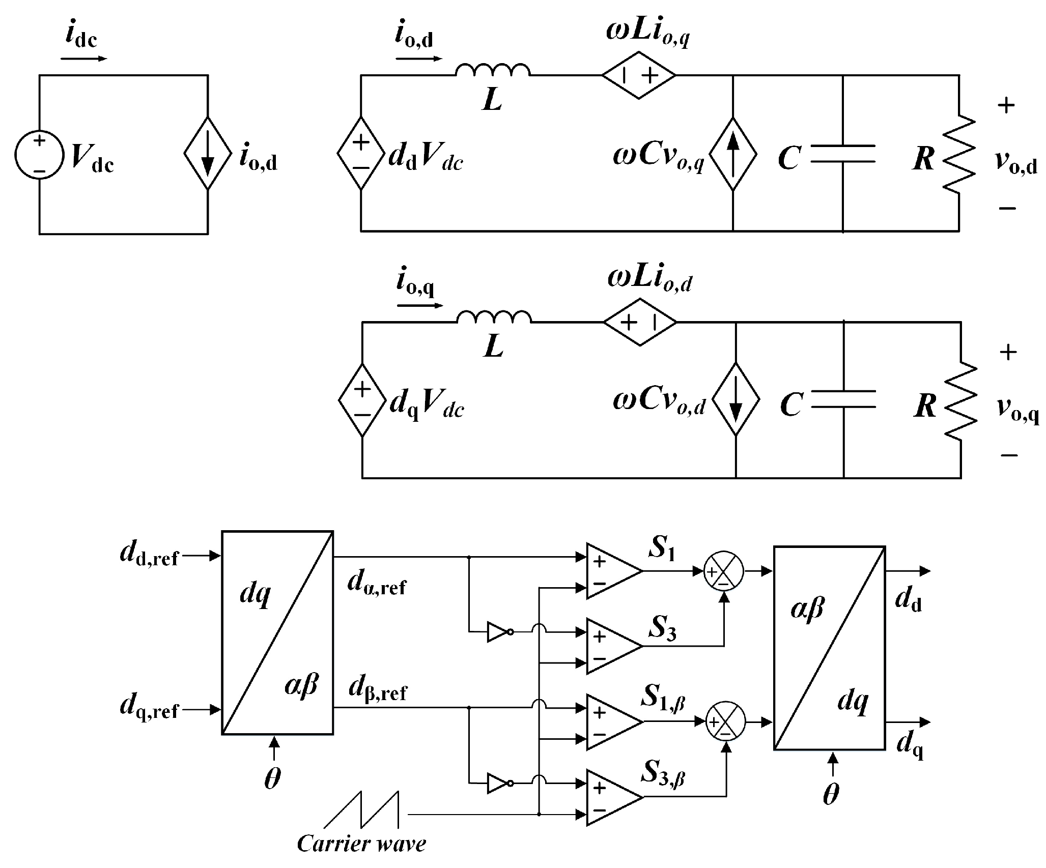
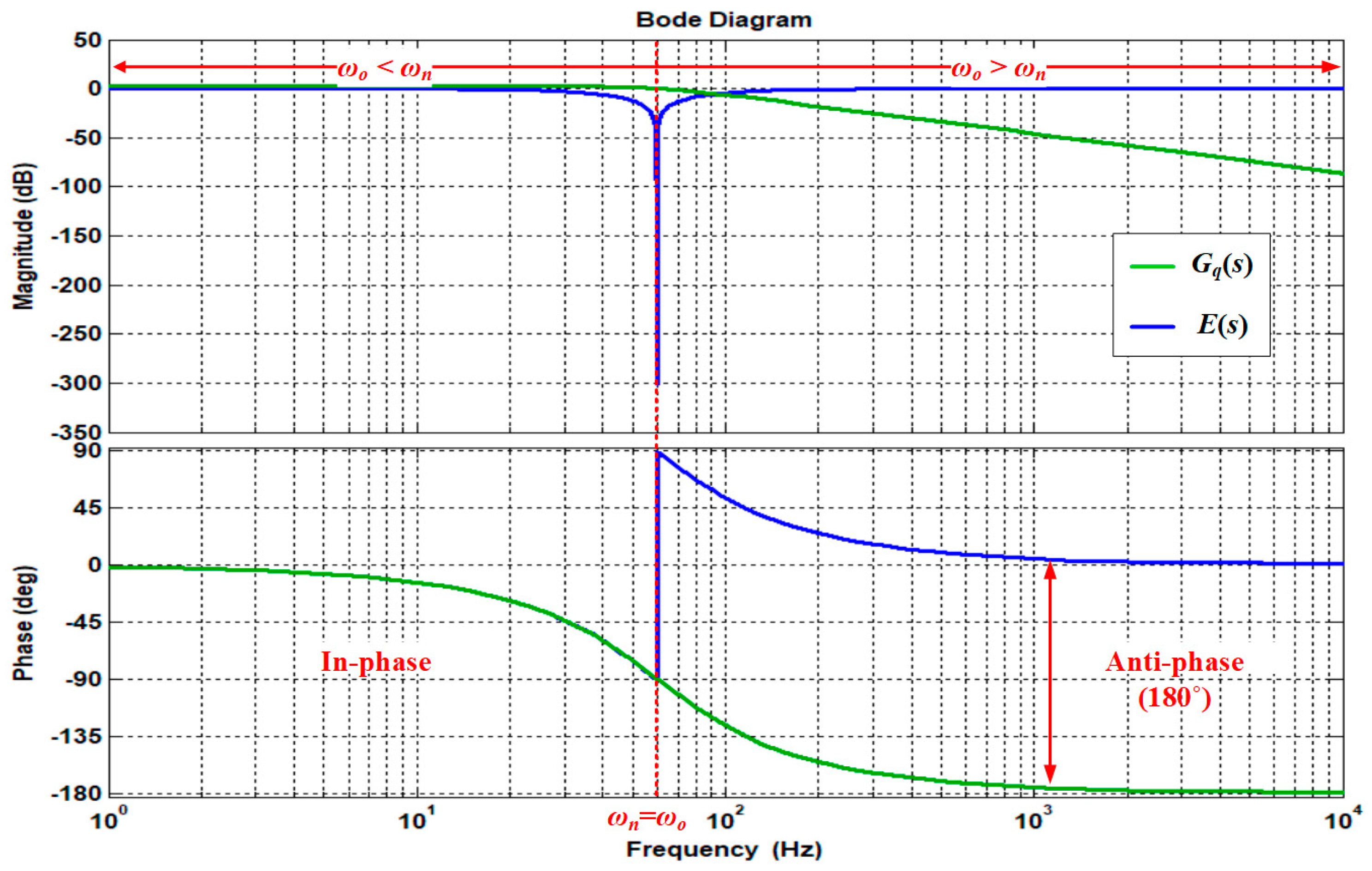
4.1. Plant Modeling Considering Unipolar Sinusoidal PWM (SPWM) in Synchronous Rotating Frame

In order to design the voltage and current controllers of the power stack, it is necessary to model the plant exactly. In this paper, plant modeling based on the synchronous rotating frame, which is commonly used to model the plant in a single-phase full-bridge inverter [14], is performed as shown in Equations (30) and (31).

$$v_{x,d}(t)=-\omega L\cdot i_{L,q}(t)+L\cdot \frac{d{i}_{L,d}(t)}{dt}+v_{o,d}(t)$$

(30)

$$v_{x,q}(t)=+\omega L\cdot i_{L,d}(t)+L\cdot \frac{d{i}_{L,q}(t)}{dt}+v_{o,q}(t)$$

(31)

Since the d-q based model enables control using the DC value in the synchronous rotating frame, the controller performance is excellent, but it has a disadvantage that it does not reflect the actual switching characteristics. Therefore, in addition to d-q based modeling, a macro model for considering unipolar SPWM is presented and included in plant modeling. In Figure 4, based on the Boolean function of power switch S_n, the output voltage v_o can be expressed using the pole voltage v_a, v_b, as follows in Equation (32).

$$v_o=v_a-v_b=S_{FB}{V}_{dc},S_{FB}\in \{1,0,-1\}$$

(32)

$$S_{FB}=\left(\frac{S_1-S_4}{2}\right)-\left(\frac{S_3-S_2}{2}\right)=S_1-S_3$$

(33)

In this case, the switching function of a full-bridge inverter is defined as the difference between S₁ and S₃ in Equation (33). In order to apply Equation (33) for reflecting the switching characteristics in Equations (30) and (31), the model was configured in a stationary α–β frame by using a d-q transformation and its inverse transformation, as shown in Figure 5. Figure 6 shows the comparison waveforms of an equivalent model where red, blue, and green solid lines represent the output voltage of the power model, equivalent switching model, and d–q equivalent model, respectively. The green solid line of Figure 6b identifies the improvement of model accuracy, in that the model reflects the switching characteristics although it is configured in a synchronous rotating frame.

4.2. SOGI-based QSG and FLL

To control the single-phase inverter in a synchronous rotating frame, an all pass filter (APF) is necessary for quadrature signal generation (QSG) in synchronous-reference-frame (SRF) voltage and current control. APF accurately delays the component of the fundamental frequency by 90°; however, the inverter-output frequency is changed from the fundamental frequency in droop control, and it can deteriorate the control performance. Therefore SOGI-FLL is adopted to realize the grid synchronization directly in the stationary reference frame. Also, SOGI-based QSG can suppress the circulating current in the parallel-operation of inverters. Equations (34)–(36) show the key transfer function of SOGI-FLL.

$$G_d(s)=\frac{k{\omega }_{o}s}{s^2+k{\omega }_{o}s+{\omega }_o{}^2}$$

(34)

$$G_q(s)=\frac{k{\omega }_o^2}{s^2+k{\omega }_{o}s+{\omega }_o{}^2}$$

(35)

$$E(s)=\frac{{\epsilon }_v(s)}{v(s)}=\frac{s^2+{\omega }_n^2}{s^2+k{\omega }_{n}s+{\omega }_n^2}$$

(36)

where ω_n, ω_o is the fundamental frequency and output of SOGI-FLL respectively and k is the gain of SOGI-FLL. The gain of SOGI-FLL k determines the damping characteristics of Equations (34) and (35), as shown in Figure 7. As k increases, the magnitude response of G_d(s) and G_q(s) become increased, resulting in the decrease of the damping ratio in the overall frequency range, but the phase response reduces in other frequency regions except for the fundamental frequency.

Figure 8 illustrates the magnitude and phase response of Equations (35) and (36). SOGI-FLL tracks the angular speed reference generated by a multinomial droop model, and the fundamental frequency of SOGI is synchronized to the droop model, improving the control performance because the fundamental frequency of APF is fixed and cannot be matched to the angular speed reference caused by the droop model. The overall control block diagram of the proposed control strategy is shown in Figure 9.

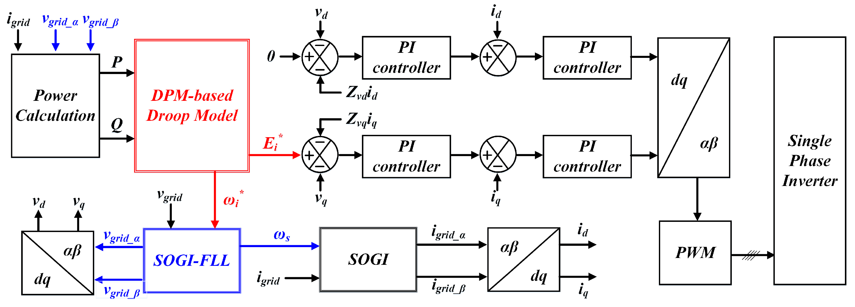
4.3. The Proposed Control Block Diagram of Droop-Controlled Parallel-Inverter

Figure 9 shows the proposed control block diagram of the droop-controlled parallel-inverter, where it can be seen that a droop control structure based on a dynamic phasor and SOGI-FLL is included in the overall control structure. The output voltage of the inverter module v_o is controlled to the reference voltage E_i^* and angular frequency ω_i^* generated by the dynamic phasor-based droop model. SOGI-FLL enables the angular frequency ω_s of the inverter system to track ω_i^*, which compensates the phase delay error caused by QSG.

On the basis of the stability analysis result obtained by applying the system parameters to the dynamic phasor-based droop model, the droop coefficients are selected, and SOGI-FLL is applied to the control structure for the purpose of robustness against frequency fluctuation caused by the droop control in a single-phase system, as shown in Figure 9.

The closed-loop control of the output voltage and current are executed separately between power stacks. The closed-loop controller for the output voltage of each inverter module will output the reference current of the current controller performing the power sharing in parallel-operation. In this case, the proposed control strategy of a droop-controlled parallel-inverter improves the power sharing and stability of an inverter-based microgrid.

In addition, in this paper, the virtual impedance is also applied to the d-q control structure to match the output impedance of the parallel-operating inverters. When designing the controller, the model of a single-phase inverter, considering unipolar SPWM in synchronous rotating frame, is used to improve the model accuracy and reflect the switching characteristics. As discussed previously, consequently, the design and control of droop-controlled parallel-inverters, according to the proposed design procedure, enable the system to achieve accurate power sharing and be stable without any communication between the inverter modules.

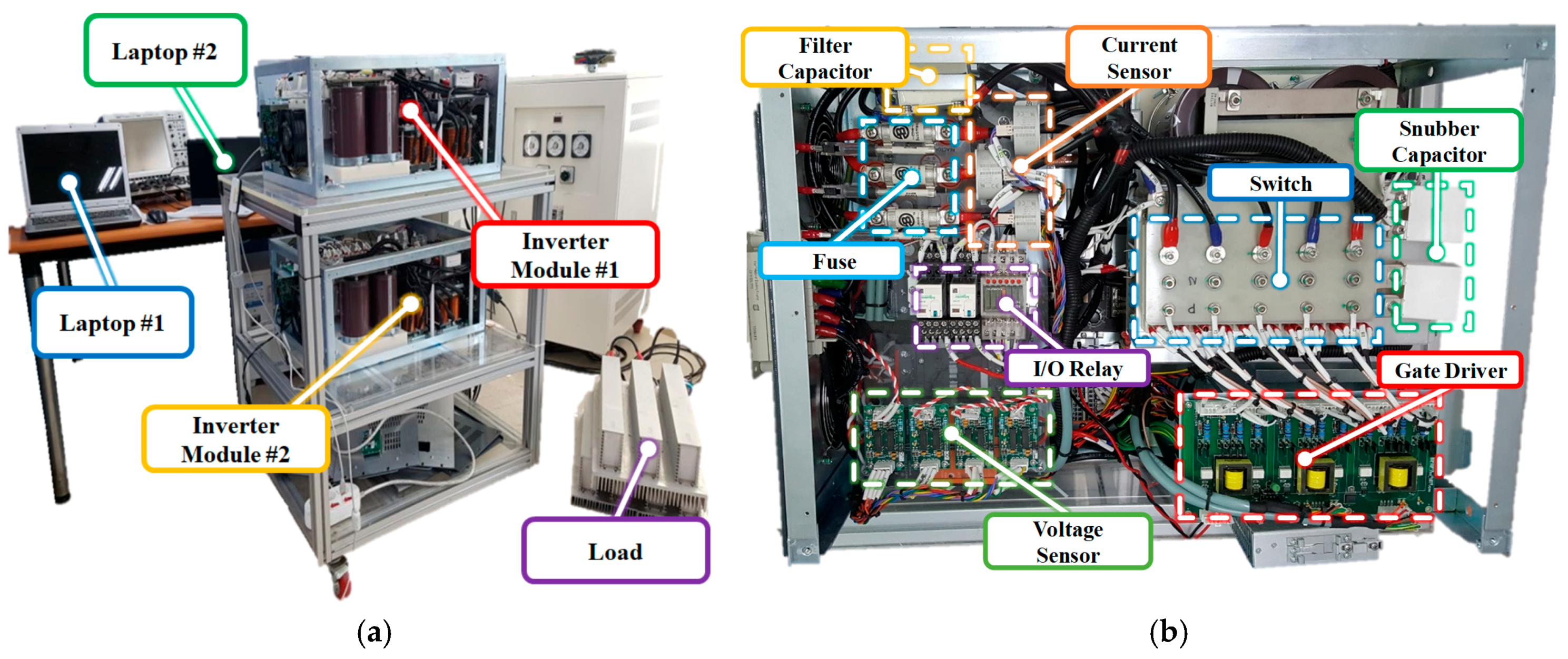
5. Implementation of Droop-Controlled Parallel-Inverter

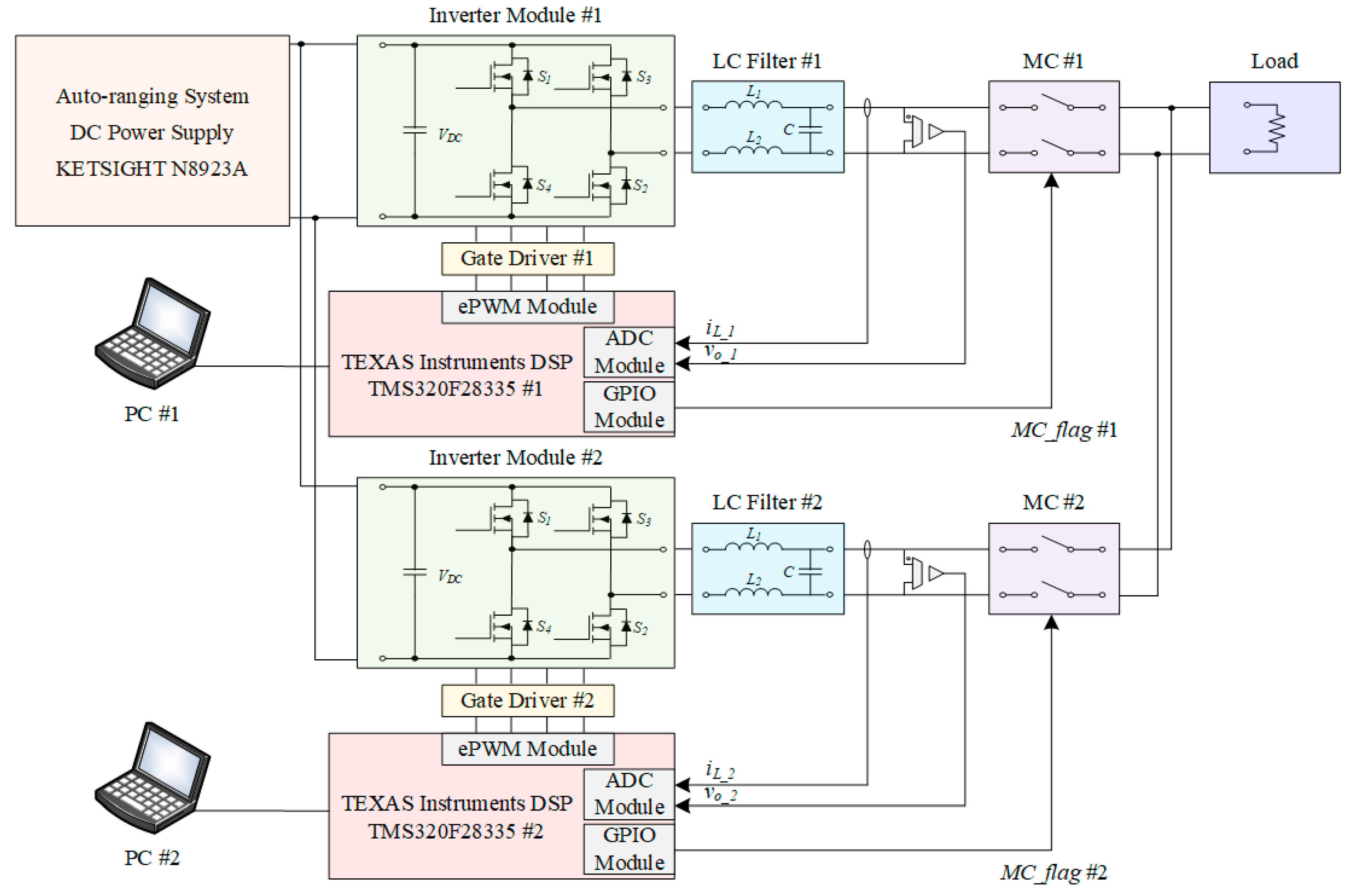
5.1. Configuration of the Experiment System

To verify the proposed dynamic-phasor based droop control in single-phase parallel-operating inverters, the configuration of droop-controlled parallel-inverters, based on the design and control of using a dynamic-phasor-based droop model and SOGI-FLL, is shown in Figure 10. Each power stack included an inverter module, L-C passive filter, AC-side magnetic contactor (MC), gate driver, and TMS320F28335-based digital controller, performing control interrupts with both an inner current control loop and an outer control loop of voltage and active/reactive power, without any communication line between power stacks, which is specifically discussed in Figure 9. The L–C filter was constructed to reduce the current harmonics, and L of the passive filter consists of the split inductor L₁, L₂ for parallel operation.

The closed-loop control of the output voltage and current were executed separately between power stacks. The closed-loop controller for the output voltage of each inverter module output the reference current of the current controller performing the power sharing in parallel-operation. In this case, the proposed control strategy of a droop-controlled parallel-inverter improved the power sharing and stability of the inverter-based microgrid.

According to Figure 10, the experimental setup was implemented as shown in Figure 11. Fuse and snubber capacitors were used to prevent the system from the damage caused by the overcurrent or overvoltage in both initial operation and transient response. Moreover, in order to prevent the control signal from the noise, an I/O relay was used in Figure 11.

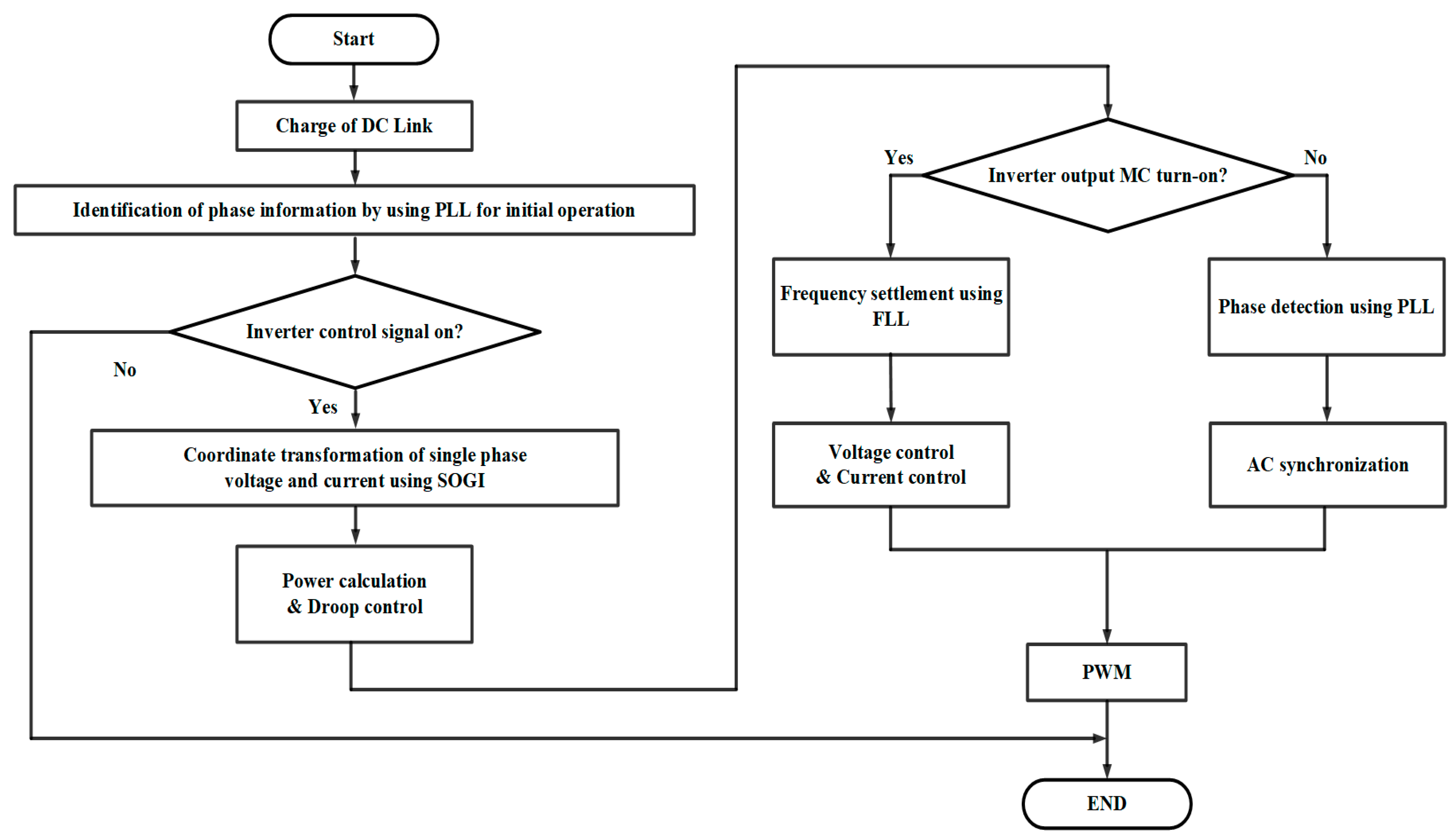
5.2. Control Sequence of Operation

In parallel operation without any communication line, the transient state which may damage the power device could be largely generated because of the asynchronization of the AC output voltage amplitude and frequency between the inverter modules; however, the difference of the voltage amplitude and frequency is minor, especially at the time of connection or disconnection of the inverter module in the case that the number of parallel-operating inverters is changed. Therefore, in order to minimize the transient response which deteriorates the stability and damage the power device, a system operation sequence that enables the stable operation in parallel is also presented in Figure 12.

Figure 12 shows the system operation sequence of a droop-controlled parallel-inverter to stably establish the AC bus of an inverter-based microgrid. First, a phase-locked loop for detecting the phase of output voltage is required to initially generate the phase information and synchronize the output voltage. It must be performed before the control sequence starts to synchronize the output voltage of the inverter, which starts to be connected or disconnected to the AC bus of the inverter-based microgrid applications. Second, identification of the control signal of the inverter module is required to determine the operation of the inverter module. Third, the process of checking, where the magnetic contactor (MC) is open or closed on the AC output terminal, is presented against the initial operation sequence where synchronization of the AC output terminal is required. The inverter starts to synchronize the amplitude and frequency of the voltage with an open-loop considering modulation index before the inverter module is connected to the AC bus, and then it is connected to the AC bus with droop control.

6. Simulation and Experimental Results

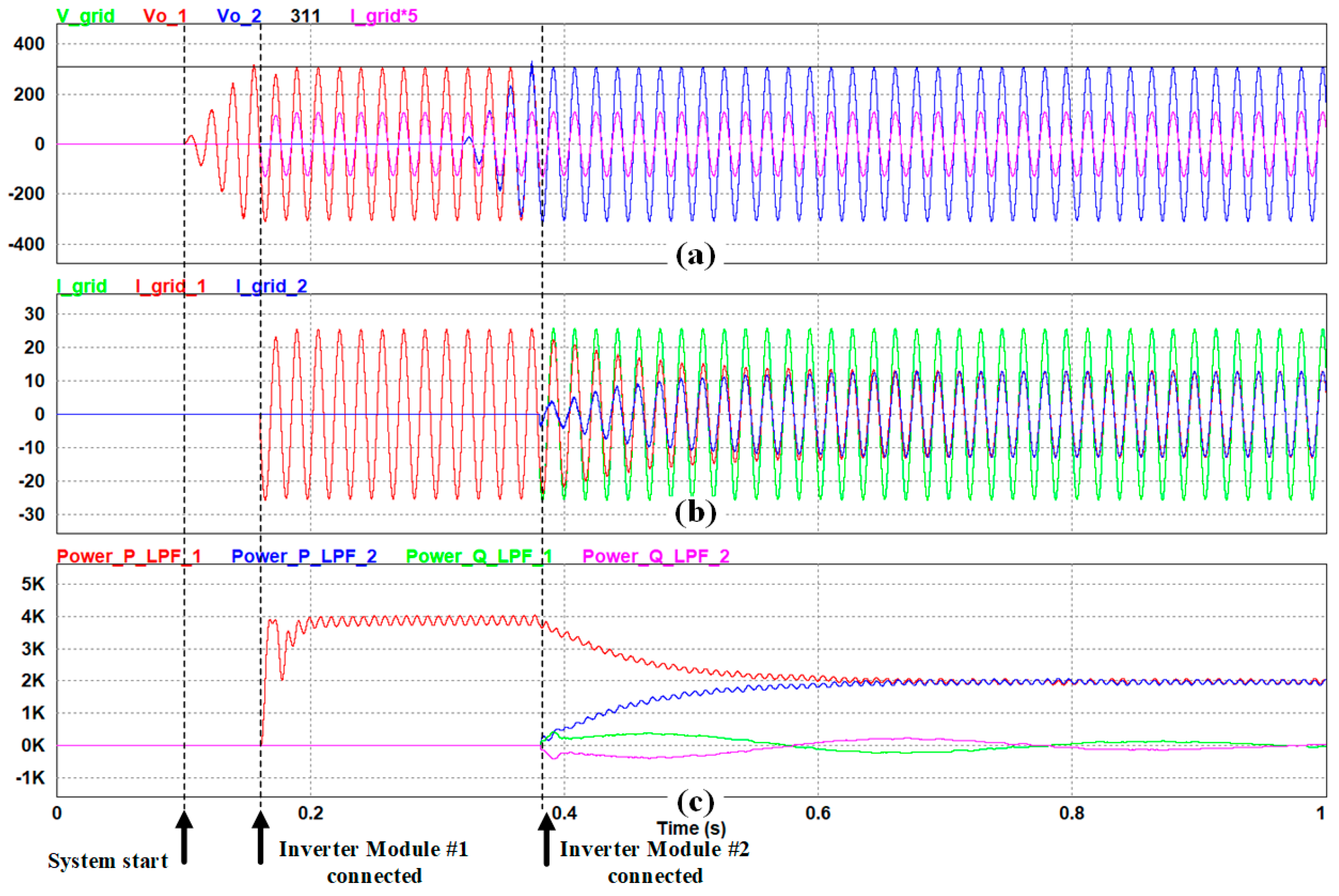
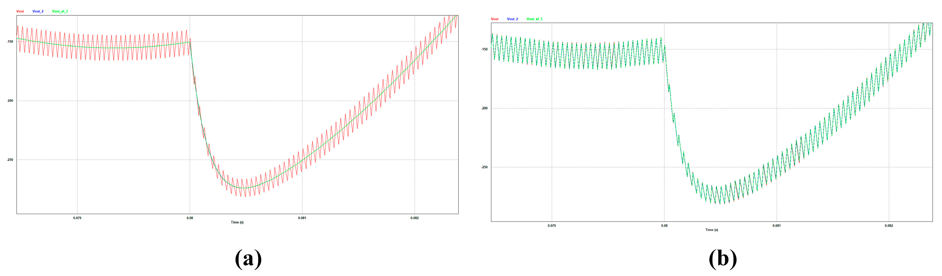
6.1. Simulation Results

To demonstrate the proposed modeling and control strategy of an inverter-based microgrid, the simulation was performed using the PSIM simulation tool. Figure 13 shows the performance of power sharing and the seamless mode when the inverter module is connected. According to the presented system operation sequence, first, one of the inverter modules starts to generate the sinusoidal output voltage for AC synchronization, considering the modulation index of the system. After that, the output MC of inverter module #1 is closed at about 0.16 s, making output current start to flow through inverter module #1. When starting parallel-operation, specifically at 0.32 s, output voltage of inverter module #2 is also generated to synchronize with the AC bus, using phase detection using PLL in Figure 13. Finally, when the output MC of inverter module #2 starts to close at 0.38 s, two inverter modules start the parallel operation according to the proposed droop control strategy. In the simulation, the THD of output current is measured to 1.867% and the difference of power sharing between modules is measured to 21.09 W in steady state.

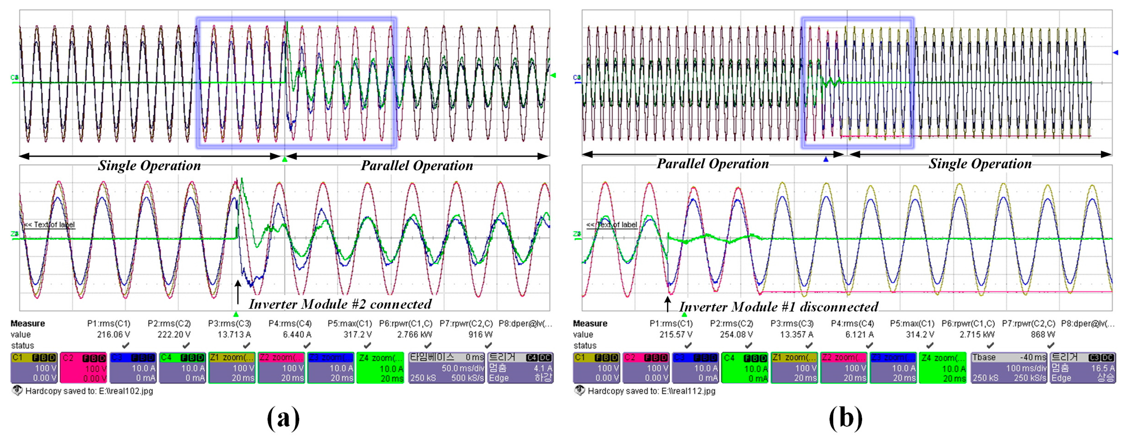
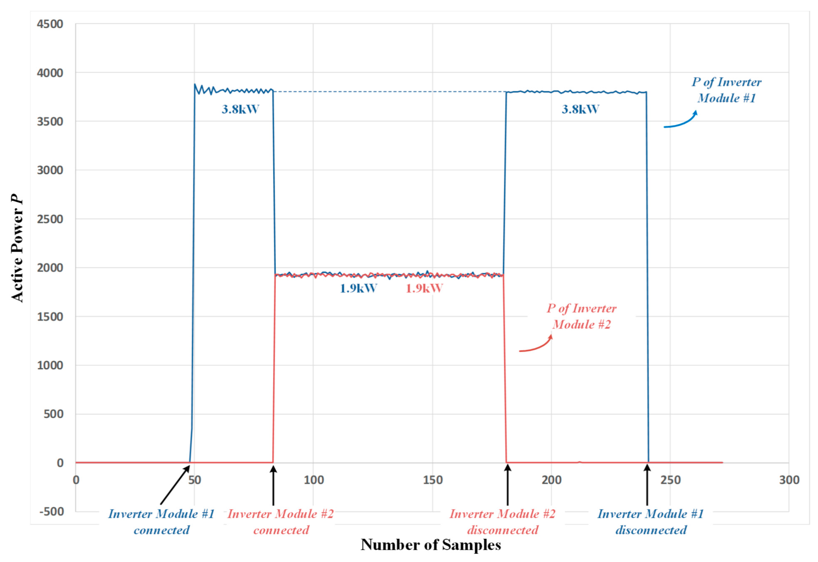
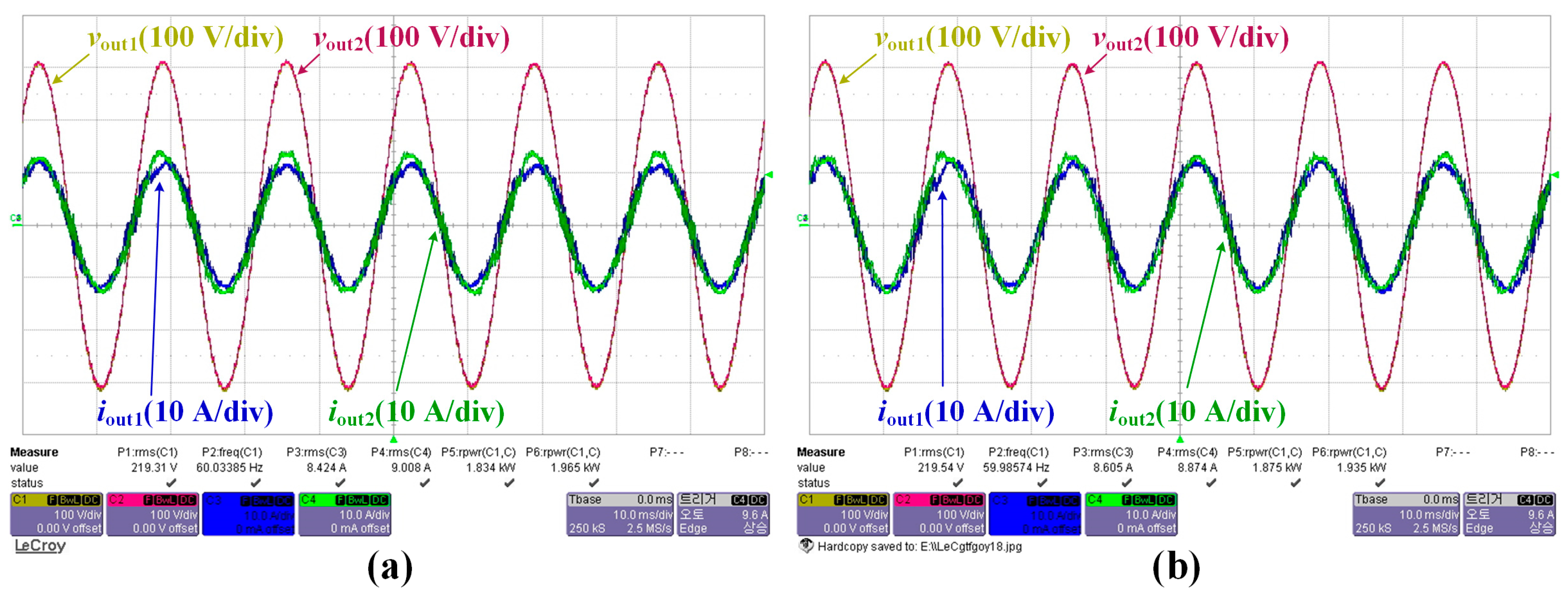
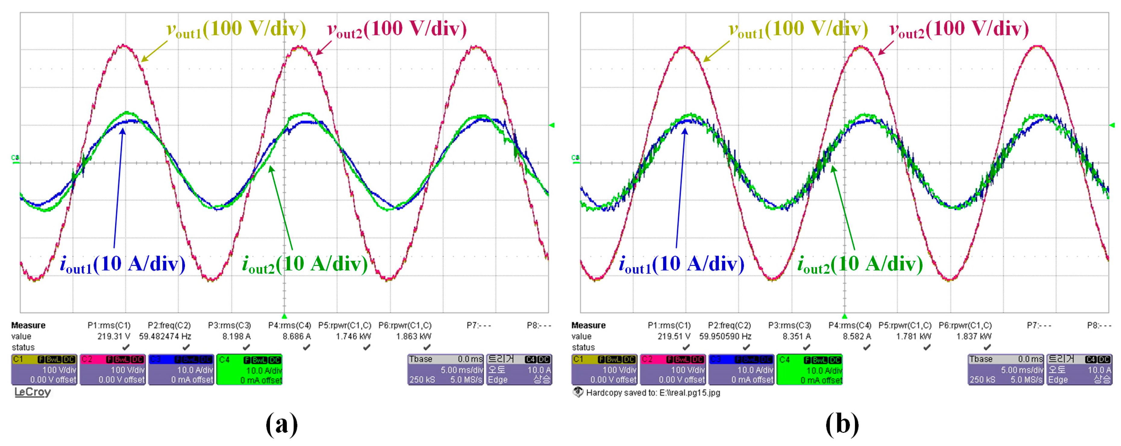
6.2. Experimental Results

To verify the validity of the proposed dynamic-phasor based modeling and control strategy, two parallel-inverters were built and combined according to the proposed design procedure for the 4-kVA prototypes. The same circuit and control parameters in Table 3 were used to compare the experimental results with simulation results.

Figure 14a,b show the experimental waveforms of output voltage and current in each inverter module using the conventional droop control and the proposed control strategy respectively with a resistive load (12.4 Ω). These experimental results illustrate that current deviation of each module was reduced from 0.584 A to 0.269 A when the proposed control strategy was applied. As a result, the deviation of active power was reduced from 131 W to 60 W as shown in Figure 14.

Figure 15a,b illustrate the experimental result of applying the conventional droop control and the proposed control strategy, respectively, with the R–L load (12.4 Ω and 6 mH). In Figure 15, when using the proposed control strategy, the current deviation was reduced from 0.488 A to 0.231 A and the power deviation was reduced from 117 W to 56 W when compared to the conventional droop control.

Consequently, when using the proposed control strategy, the differences in active power are 60 W and 95 W in R and R–L load, respectively, as shown in Figure 13b and 14b, respectively. Conversely, the power sharing ratios of Figure 14b are 98.42% and 101.58% while those of Figure 14a are 96.55% and 103.45% in resistive load. Furthermore, the power sharing ratios of Figure 15b are 98.45% and 101.55% while those of Figure 15a are 96.76% and 103.24%.

Figure 16 shows the experimental waveforms of the proposed control strategy in mode transfer, where the inverter module starts to be connected or disconnected to the AC bus. Figure 16a illustrates the waveform of the transient response in which one inverter is running and the second inverter is connected to AC bus, resulting in parallel-operation with droop control. Figure 16b shows the waveform of the transient response in which two inverters are operated in parallel and one inverter is disconnected while only one inverter operates.

The graph of the active power according to the number of samples, by taking the value of active power output of two computers with a sampling frequency of 1 Hz by utilizing the graph window function of code composer studio (CCS), is shown in Figure 17. Specifically, Figure 17 shows the waveforms of active power shared by each inverter module when each module is connected or disconnected.

These results demonstrate and verify the validity of the proposed dynamic phasor-based droop-controlled inverter and SOGI-FLL in terms of improvement of the power sharing ratio and the stability of the system.

7. Conclusions

This paper proposes the design and implementation of droop-controlled single-phase parallel-inverters based on a dynamic phasor approach in microgrid applications. The proposed droop control structure is analyzed and modeled using a dynamic phasor, and it is used to determine the dynamic stability of the power controller. Furthermore, theoretical analysis and principles of the proposed control strategy are mathematically specified and derived in this paper. The plant modeling for controller design is also presented considering the unipolar SPWM to improve the model accuracy and control performance in a synchronous rotating frame. Moreover, SOGI-FLL is applied to contribute the minimization of inherent tradeoff in inverter-based droop-controlled islanded microgrid applications, and it is also included in the proposed droop control structure. Furthermore, the control sequence of operation is presented to implement the actual operation of parallel operation of single-phase inverters.

Consequently, this paper contributes to the design of the droop-controlled parallel-inverter by considering the design factors required for the implementation of parallel-inverters, such as stability analysis, digital filtering, the control sequence for network synchronization, and so on. In order to demonstrate the validity of this paper, two parallel-inverters were developed and implemented in accordance with the proposed design procedure for the 4-kVA prototypes.

The proposed control method and feasibility were demonstrated using 4-kVA prototypes, showing that the measured power sharing ratios of each inverter module using the proposed control strategy are 98.42% and 101.58% while those using the existing droop control are 96.55% and 103.45% in resistive load, and those of each inverter module in R–L load are 98.45% and 101.55% while those using the existing droop control are 96.76% and 103.24%. Given the simulation and experimental results, the validity and effectiveness of this paper are proven and demonstrated.

References

1. Kai, Y.; Ai, Q.; Wang, S.; Ni, J.; Lv, T. Analysis and optimization of droop controller for microgrid system based on small-signal dynamic model. IEEE Trans. Smart Grid 2016, 7, 695–705. [Google Scholar]
2. Guerrero, J.M.; Vasquez, J.C.; Matas, J.; de Vicuna, L.G.; Castilla, M. Hierarchical control of droop-controlled AC and DC microgrids—A general approach toward standardization. IEEE Trans. Ind. Electron. 2011, 58, 158–172. [Google Scholar] [CrossRef]
3. Dou, C.; Zhang, Z.; Yue, D.; Gao, H. An Improved Droop Control Strategy Based on Changeable Reference in Low-Voltage Microgrids. Energies 2017, 10, 1080. [Google Scholar] [CrossRef]
4. Zhong, Q.-C.; Zeng, Y. Universal droop control of inverters with different types of output impedance. IEEE Access 2016, 4, 702–712. [Google Scholar] [CrossRef]
5. Chaitanya, N.; Sekhar, K.C.; Anjaneyulu, K.S.R. Integrated power management strategy of parallel inverters for distributed generation system. In Proceedings of the IEEE International Conference on Advanced Communication Control and Computing Technologies (ICACCCT), Ramanathapuram, India, 25–27 May 2016. [Google Scholar]
6. Han, Y.; Li, H.; Shen, P.; Coelho, E.A.A.; Guerrero, J.M. Review of active and reactive power sharing strategies in hierarchical controlled microgrids. IEEE Trans. Power Electron. 2017, 32, 2427–2451. [Google Scholar] [CrossRef]
7. Zhong, Q.-C. Robust droop controller for accurate proportional load sharing among inverters operated in parallel. IEEE Trans. Ind. Electron. 2013, 60, 1281–1290. [Google Scholar] [CrossRef]
8. Kim, J.-H.; Lee, Y.-S.; Kim, H.-J.; Han, B.-M. A New Reactive-Power Sharing Scheme for Two Inverter-Based Distributed Generations with Unequal Line Impedances in Islanded Microgrids. Energies 2017, 10, 1800. [Google Scholar] [CrossRef]
9. Li, D.; Zhao, B.; Wu, Z.; Zhang, X.; Zhang, L. An Improved Droop Control Strategy for Low-Voltage Microgrids Based on Distributed Secondary Power Optimization Control. Energies 2017, 10, 1347. [Google Scholar] [CrossRef]
10. Guerrero, J.M.; de Vicuna, L.G.; Matas, J.; Castilla, M.; Miret, J. Output impedance design of parallel-connected UPS inverters with wireless load-sharing control. IEEE Trans. Ind. Electron. 2005, 52, 1126–1135. [Google Scholar] [CrossRef]
11. Matas, J.; Castilla, M.; de Vicuña, L.G.; Miret, J.; Vasquez, J.C. Virtual impedance loop for droop-controlled single-phase parallel inverters using a second-order general-integrator scheme. IEEE Trans. Power Electron. 2010, 25, 2993–3002. [Google Scholar] [CrossRef]
12. Alberto, C.-M.; Pérez-Cisneros, M.A.; Domínguez-Navarro, J.A.; Osuna-Enciso, V.; Zúñiga-Grajeda, V.; Gurubel-Tuna, K.J. Dynamic phasors modeling for a single phase two stage inverter. Electr. Power Syst. Res. 2016, 140, 854–865. [Google Scholar]
13. Piyasinghe, L. Dynamic Phasor Based Analysis and Control in Renewable Energy Integration; University of South Florida: Tampa, FL, USA, 2015. [Google Scholar]
14. Roshan, A.; Burgos, R.; Baisden, A.C.; Wang, F.; Boroyevich, D. A DQ frame controller for a full-bridge single phase inverter used in small distributed power generation systems. In Proceedings of the APEC 2007-Twenty Second Annual IEEE Applied Power Electronics Conference, Anaheim, CA, USA, 25 February–1 March 2007. [Google Scholar]
15. Turhan, D.; Andersson, G. Comparison of the efficiency of dynamic phasor models derived from ABC and DQO reference frame in power system dynamic simulations. In Proceedings of the 7th IET International Conference on Advances in Power System Control, Operation and Management (APSCOM 2006), Hong Kong, China, 30 October–2 November 2006; p. 204. [Google Scholar]
16. Adarsh, N.; Ayyanar, R. Dynamic phasor model of single-phase inverters for analysis and simulation of large power distribution systems. In Proceedings of the IEEE 4th IEEE International Symposium on Power Electronics for Distributed Generation Systems (PEDG), Rogers, AR, USA, 8–11 July 2013. [Google Scholar]
17. Kulasza, M. Generalized Dynamic Phasor-Based Simulation for Power Systems. Master’s Thesis, University of Manitoba, Winnipeg, MB, Canada, 13 January 2015. [Google Scholar]
18. Zhong, Q.; Shi, Q.; Wang, G.; Li, H. Short circuit analysis of PV inverter under unbalanced conditions with dynamic phasor sequence components. In Proceedings of the IEEE Power and Energy Society General Meeting (PESGM), Boston, MA, USA, 17–21 July 2016. [Google Scholar]
19. Guo, X.; Lu, Z.; Wang, B.; Sun, X.; Wang, L.; Guerrero, J.M. Dynamic phasors-based modeling and stability analysis of droop-controlled inverters for microgrid applications. IEEE Trans. Smart Grid 2014, 5, 2980–2987. [Google Scholar] [CrossRef]
Figure 1. Schematic diagram of droop-controlled inverter-based MG.
Energies 11 01683 g001
Figure 2. The conventional droop model of inductive output inverter according to (a) P-ω and (b) Q-E curve.
Energies 11 01683 g002
Figure 3. Stability determination of dynamic phasor model-based droop-controlled inverter with change of (a) droop coefficient KP, (b) droop coefficient KQ, and (c) cutoff frequency ωf.
Energies 11 01683 g003
Figure 4. Equivalent circuit model of single-phase full-bridge inverter.
Energies 11 01683 g004
Figure 5. Equivalent plant model of single-phase full-bridge inverter considering unipolar SPWM in synchronous rotating frame.
Energies 11 01683 g005
Figure 6. Magnified output voltage waveforms of equivalent model of (a) conventional d-q model and (b) the presented plant model considering unipolar SPWM in synchronous rotating frame.
Energies 11 01683 g006
Figure 7. Bode diagram of transfer functions (a) Gd(s) and (b) Gq(s).
Energies 11 01683 g007
Figure 8. Bode diagram of SOGI-FLL.
Energies 11 01683 g008
Figure 9. Control block diagram of droop-controlled parallel-inverter using the proposed control strategy.
Energies 11 01683 g009
Figure 10. Control block diagram of droop-controlled parallel-inverter using the proposed control strategy.
Energies 11 01683 g010
Figure 11. (a) Experimental setup consisting of two parallel-inverters; (b) each power stack.
Energies 11 01683 g011
Figure 12. System operation sequence of droop-controlled parallel-inverter.
Energies 11 01683 g012
Figure 13. Simulation waveform of (a) grid voltage, (b) grid current, (c) and active and reactive power.
Energies 11 01683 g013
Figure 14. Experimental waveforms of using (a) conventional droop control and (b) the proposed control strategy with resistive load (12.4 Ω).
Energies 11 01683 g014
Figure 15. Experimental waveforms of using (a) conventional droop control and (b) the proposed control strategy with R–L load (12.4 Ω + 6 mH).
Energies 11 01683 g015
Figure 16. Experimental waveforms of using the proposed control strategy in transient period of inverter module (a) connected and (b) disconnected without any communication.
Energies 11 01683 g016
Figure 17. Experimental result of active powers of each inverter module in using the proposed control strategy.
Energies 11 01683 g017