Strategic Behavior of Retailers for Risk Reduction and Profit Increment via Distributed Generators and Demand Response Programs

Abstract

Following restructuring of power industry, electricity supply to end-use customers has undergone fundamental changes. In the restructured power system, some of the responsibilities of the vertically integrated distribution companies have been assigned to network managers and retailers. Under the new situation, retailers are in charge of providing electrical energy to electricity consumers who have already signed contract with them. Retailers usually provide the required energy at a variable price, from wholesale electricity markets, forward contracts with energy producers, or distributed energy generators, and sell it at a fixed retail price to its clients. Different strategies are implemented by retailers to reduce the potential financial losses and risks associated with the uncertain nature of wholesale spot electricity market prices and electrical load of the consumers. In this paper, the strategic behavior of retailers in implementing forward contracts, distributed energy sources, and demand-response programs with the aim of increasing their profit and reducing their risk, while keeping their retail prices as low as possible, is investigated. For this purpose, risk management problem of the retailer companies collaborating with wholesale electricity markets, is modeled through bi-level programming approach and a comprehensive framework for retail electricity pricing, considering customers’ constraints, is provided in this paper. In the first level of the proposed bi-level optimization problem, the retailer maximizes its expected profit for a given risk level of profit variability, while in the second level, the customers minimize their consumption costs. The proposed programming problem is modeled as Mixed Integer programming (MIP) problem and can be efficiently solved using available commercial solvers. The simulation results on a test case approve the effectiveness of the proposed demand-response program based on dynamic pricing approach on reducing the retailer’s risk and increasing its profit.

1. Introduction

During the early stages of the electricity market formation, competition only existed on the wholesale level; such that large producers were submitting their electricity production offers to the wholesale market and distribution companies were submitting the aggregated electrical demand of their customers. However, following the electricity market development and with the aim of achieving a perfectly competitive electricity market, retail electricity market was established [1]. Under this situation, retailers are in business to bridge the gap between wholesale electricity markets and small electricity consumers who do not actively participate in the wholesale electricity markets.

The retailer, according to the strategy it implements, determines the contractual electricity prices for its customers. In case the retailer designates inappropriate prices, it may face economic losses or may lose a number of its customers. In other words, the strategy of a retailer to determine electricity prices and to decide on its contracts has a direct impact on its capability to attract more customers [2]. A retailer should purchase electricity through forward contracts or directly from centralized electricity markets and sell it through contracts, usually with constant price, to its customers [3,4]. Network constraints are basically outside the transaction model of the retailers. The retailers are supposed to share their transactions’ data to the distribution network operator where they are located. Afterwards, the distribution network operator performs a power flow program with respect to the initial schedules of all the retailers, distributed generators, and other power sources/demands connected to its network, to assure the feasibility of the transactions. The active and reactive power flow model in distribution networks, with distributed energy sources, have been widely investigated in the literature [5,6,7,8,9,10]. In case no network constraint is violated, the distribution network operator finalized the transactions. Otherwise, the network operator and retailers will coordinate to resolve the violations and bring the network condition to the safe boundary.

In [11,12], the authors studied the formation of retail electricity markets and investigated the competition in the retail markets. In reference [13], the economic problem of retailer has been investigated. In this regard, the concepts of customers’ welfare in the retail electricity markets, value-added of retail market formation, and economic benefits of this market have been analyzed. Reference [14] for the first time investigated the problem of demand-side participation in electricity markets from different perspectives and analyzed some issues including price elasticity of electricity demand and its impact on the electricity prices, different manners to sell electricity in retail level, and different methods of electricity procurement for retailers. Players’ behavior in a deregulated competitive electricity market is discussed in [15]. In reference [16], the approaches implemented by retailers for load forecasting have been studied. Reference [17] modeled the retailer’s problem through Monte-Carlo method and dynamic programming approach.

Due to the stochastic behavior of the electricity market prices, market participation incorporates inherent risks for all market players, including the retailers. Hence, financial risks of market participation should also be considered in retailers’ decision-making problem. Risk management is the process of reducing probability of adverse effects of an activity through conscious actions for predicting unplanned contingencies and planning to avoid them. Risk management problem in electricity and fuel markets was discussed in [18,19]. In references [20,21], the risk of offering high electricity prices by producers to day-ahead market was evaluated and the producers’ strategy in electricity pricing was modeled. Hatami et al. [22] developed a mathematical model to maximize the retailer’s profit and minimize its risks, simultaneously, by using the measure of Conditional Value at Risk (CVaR) for modeling profit in the objective function of the retailer. For considering the uncertainty in PV generated power and electricity price the CVaR is used in [23]. Reference [24] provided useful information for market participants, e.g., suppliers and consumers, for evaluating the contracts from the economic perspective [3].

One of the most efficient approaches that a retailer can consider to eliminate the uncertainties and to reduce its risk is to implement Demand Response programs (DRPs). Through DRPs, retailer provides incentives to its customers to change their normal electricity consumption patterns and shift their flexible demand from peak hours to off-peak hours. According to the definition of Department Of Energy (DOE), DR is the ability of industrial, commercial, and residential customers to refine their electrical energy demand profiles during peak-load hours with the aim of achieving reasonable prices and improving system reliability [25,26]. Different DR schemes in electricity markets were investigated by Valero et al. in [27]. In [28], the mathematical model of different DRPs are provided and a comparison among these models is performed to find the best option in terms of modifying the initial load curve. In a general sense, DRPs are employed for making conversions in electricity consumption profile of consumers. Significant growth of electricity demand makes DRPs more attractive for both electricity consumers and system operators [29,30]. DRPs can be divided into three general categories: Time-Based Programs (TBP), Incentive-Based Programs (IBP), and Market-Based Programs (MBP), which have been discussed widely in the literature [31,32,33,34]. From the DR participation aspect, the market participants can be divided into DR buyers (DRBs) and DR Service Providers (DRSPs). Besides the retailers, other power system entities also derive benefits from DRPs, including transmission system owners, distribution systems, and aggregators [35,36]. In [37], the problem of electricity distribution and pricing by retailers, considering DRPs and electricity market price uncertainty, have been discussed. Reference [12] provided an integrated framework for determining electricity price to consumers, based on time-based pricing and contract management.

Most of the previous studies investigated above, concentrated on the concept and modeling of the DRPs; while, only a few of them considered DR as a commodity to be directly transacted among DRSPs and DRBs. Furthermore, few researchers have addressed the impact of DR applications on increasing the profit of retailers and the potential decrease of retail prices for final customers. Reference [38] models a reward-based DRP in energy procurement plans of retailer. The DRP in [39] assumes that offering higher rewards by the retailer is followed by stepwise demand decrease by customers, while the costs minimization of customers is not modeled in the retailer’s decision-making problem.

One of the emerging research areas in the retail electricity industry is Dynamic Pricing which is a demand-side management technique to reduce peak load and manage consumers load profile through setting different prices at different time periods [39]. Dynamic pricing not only can cease large investments by shifting demand from peak hours to off peak, but also provides consumers with an opportunity to reduce their electricity bills at a constant electricity consumption. Dynamic pricing approach includes a variety of pricing mechanisms, e.g., Critical Peak Pricing (CPP), Time- of-Use (TOU) pricing, and Real Time Pricing (RTP).

In this paper, we model the retailer’s medium-term planning for optimal involvement in the future contracts and spot electricity markets, as well as optimum pricing of electricity for its clients. The expected profit of the retailer from electricity trading is maximized, incorporating the risk aversion by limiting the volatility of the expected profit through Conditional Value at Risk (CVaR) parameter. The retailer is supposed to pre-determine three prices to its clients in their contracts, i.e., average selling price, minimum selling price, and maximum selling price. This constitutes a proper tradeoff between the retailer’s flexibility in defining dynamic prices and its clients’ risk to face high hourly prices. Without loss of generality, we perform the model on a case study with the planning horizon of one week. The planning horizon contains totally 168 hourly periods. The uncertainty of spot electricity market prices and consumption data of the customers are accounted. The proposed programing problem is modeled as a bi-level problem and converted to a single-level mixed integer linear problem which can be efficiently solved using available commercial branch-at-cut solvers.

In summary, the contributions of this paper are as follows:

• Providing a detailed mathematical formulation for retailers’ decision-making problem, considering the possibility of the retailer to provide energy from forward contracts, spot electricity market, distributed generators, and demand response program;
• Modeling dynamic pricing approach by retailers as a demand-side management technique to modify customers’ load profile;
• Considering the customers’ welfare within the retailer’s decision-making problem through bi-level programming in which the first level is the retailer’s profit maximization, including the risk factor in the objective function, and the second level is customers’ cost minimization.
• Performing the proposed decision–making model on a test-case, considering the uncertainty of spot electricity prices and electricity demand, for a 1-week (168 h) period to show the effectiveness of the demand response program on the retailer’s profitability and risk;

After this introduction, Section 2 presents the mathematical model for retailers’ decision-making problem, including the problem constraints, as well as the solution approach. In Section 3 the case study and the simulation results on the case study are provided and discussed. Finally, Section 4 provides the most important conclusions of the presented work.

2. Modeling the Retailer’s Decision-Making Problem

In the previous section, the basic concepts related to the retailer problem have been introduced and a short literature review have been provided. Retailer needs to schedule its optimum involvement in the forward contracts and spot electricity markets, as well as the optimum selling price to its clients, in advance. The Conditional Value at Risk (CVaR) is selected as the measure of risk in this study to incorporate the risk aversion of the retailer into the model. In this section, first the decision-making problem of retailer is defined and the problem assumptions are presented. Then, the strategy of retailer for participating in forward electricity markets in a mid-term horizon, with the aim of making optimum contracts, through DRPs and dynamic pricing of electricity for end-use customers, will be determined. In what follows, a model for retailers’ decision-making problem is proposed and the problem constraints, as well as solution approach, is provided.

The decision-making problem of this paper is based on the underlying assumptions regarding the retailer’s condition and scheduling horizon, as follows.

The retailer is only responsible for supplying the electricity demand of its own customers;

The retailer can provide the required electricity for its customers from either wholesale electricity market or the Distributed Generators (DGs) connected to the network;

The retailer has the opportunity to make Bilateral Contracts, Put Options, and Call Options, in advance. These contracts are considered specified in the beginning of the scheduling horizon;

Since the problem is defined for mid-term scheduling horizon, day-ahead, intraday, and real-time markets are combined and considered as one spot market in the model;

The wholesale electricity spot market prices are assumed as the prices at the transmission node to which the retailer in connected. Hence, the transmission cost is included in the electricity prices.

2.1. Uncertainty Modeling

Retailers expose to variety of uncertainties in their decision-making process. These uncertainties can be divided into two general categories: (1) The uncertainties that are resulted by market transactions of retailers in the wholesale electricity markets, e.g., day-ahead and real-time electricity prices; (2) the uncertainties that are resulted by the interactions among the retailer and its customers, e.g., electricity consumption.

In this paper, the uncertainty of wholesale spot electricity prices and end-use electricity consumption are considered in the retailer’s decision-making model. The total number of scenarios is calculated by multiplying the number of scenarios regarding hourly spot electricity prices into the number of scenarios for hourly electricity consumption level.

$$N_{\omega }=N_{\omega }^{\rho }{N}_{\omega }^P$$

(1)

In the Equation (1), $N_{\omega }^{\rho }$ presents the number of price scenarios, $N_{\omega }^p$ presents the number of electricity consumption scenarios, and $N_{\omega }$ is the total number of uncertainty scenarios. Accordingly, the number of total scenarios may reach a significantly high value which in turn increases the size and running time of the program. Therefore, the fast forward and backward scenario reduction method is implemented in this study to reduce the number of scenarios.

Similarly, the probability of each scenario is calculated by multiplying the probabilities of corresponding price scenario and electricity consumption scenario.

$${\gamma }_{\omega }={\gamma }_{\omega }^{\rho }{\gamma }_{\omega }^P$$

(2)

In the Equation (2), ${\gamma }_{\omega }^{\rho }$ and ${\gamma }_{\omega }^P$ represent the probability of each price scenario and consumption scenario, respectively. ${\gamma }_{\omega }$ is the probability of the equivalent scenario.

2.2. Risk Aversion of Retailer

The risk of participating in electricity market is the most significant financial risk that a retailer confronts with. Occasionally, market participants employ forward and option contracts in order to confront the financial risks derived from uncertainty of spot market prices. In other words, applying forward and option contracts in forward electricity markets is the fundamental approach to control the risk of electricity producers and consumers in the market. These contracts in the proposed model include: Bilateral contracts, Put Option, and Call Option.

Under the bilateral contracts, contract correspondents compromise on providing a certain power quantity with a certain price during a certain time interval and both the seller and the purchaser ought to fulfill the contract [40]. Under the put option, contract correspondents compromise on providing a certain power quantity with a certain price during a certain period of time, as well. However, the seller has the option to make a decision on implementing the agreement or not, until a specific time before the contract time interval. The power provider makes this decision based on his anticipation of the sport electricity prices [41,42]. On the contrary, call option authorizes the purchaser to decide on implementing the agreement or not, before a predetermined time limit and based on his anticipation of the spot electricity market prices during the contract time period [43].

2.3. Problem Formulation

The decision-making problem of the retailer is modeled as a bi-level optimization problem. The first-level (leader’s problem) objective function is comprised of two terms: profit term, and risk term.

In the second level, regarded as the follower’s problem, demand response program along with dynamic pricing approach is implemented on the customers’ side. For this purpose, it is assumed that the retailer provides the hourly retail prices to its customers based on the predefined contracted maximum, minimum and average prices and the customers use these price data to manage their hourly electrical energy consumption.

2.3.1. First-Level Problem

The first level, regarded as the leader’s problem, aims at maximizing the retailer’s profit and simultaneously minimizing the risks.

Profit Function

The profit function of the leader’s problem (first level) presented by (3).

$$\mathsf{\Pi }=\mathcal{R}-C^{Bi}-C^{PO}-C^{CO}-C^{DG}-C^{SM}-C^{con}$$

(3)

The first term of the profit function (3) denotes the revenue of the retailer which in general is obtained from selling active and reactive electrical power to its customers. Other six terms of the profit function correspond to the variable, semi-variable, and constant costs of the retailer. The constant and semi-variable costs of the retailer, denoted by $C^{con}$, include personnel costs, cots of communication infrastructure expansion, selling costs, and etc. The variable costs of retailer include cost of providing energy through bilateral contracts $\left(C^{Bi}\right)$, cost of providing energy from put options $\left(C^{PO}\right)$, cost of providing energy through call options $\left(C^{CO}\right)$, cost of generating electrical energy from the distributed generators $\left(C^{DG}\right)$, and cost of buying energy from the spot market $\left(C^{SM}\right)$.

REVENUE OF THE RETAILER

The retailer’s revenue from selling active and reactive power is calculated in (4).

$$\mathcal{R}={\displaystyle \sum }_{t=1}^T{\displaystyle \sum }_{\omega =1}^{N_{\omega }}\gamma \left(\omega \right)\left[{\rho }^{P.FX}\left({\displaystyle \sum }_{r=1}^{Ncus}{D}_{r,t}^P\left(\omega \right)\right)+{\rho }^{Q.FX}\left({\displaystyle \sum }_{r=1}^{Ncus}{Q}_{r,t}^P\left(\omega \right)\right)\right]$$

(4)

$D_{r,t}^P\left(\omega \right)$ and $Q_{r,t}^P\left(\omega \right)$ denote the Active and reactive power consumption of customer $r$ at time period $t$ under scenario $\omega$, respectively

The variable cost terms of the objective function (4) are presented as follows.

COST OF BILATERAL CONTRACTS

Bilateral contracts play an important role in providing the electrical power, especially base-load power, for the retailers. Equation (5) states the costs of bilateral contracts for the retailers.

$$C^{Bi}={\displaystyle \sum }_{1=t}^T{\displaystyle \sum }_{i=1}^{NBi}{P}_i^{Bi}{\rho }_i^{Bi}{\delta }_{i,t}^{Bi}$$

(5)

The offer function of bilateral contracts is modeled as staircase function defined by a minimum power $P_i^{Bi.min}$ and incremental power $\left(\Delta P_i^{Bi}\right)$ for each block of the offered power. Total offer blocks of each bilateral contract is denoted by $M_i^{Bi}.$ Power transacted through bilateral contracts is enforced by (6).

$$P_i^{Bi}\in \left\{0,P_i^{Bi.min},P_i^{Bi.min}+\Delta P_i^{Bi},\dots ,P_i^{Bi.min}+M_i^{Bi}\Delta P_i^{Bi}\right\}$$

(6)

Figure 1 illustrates the staircase offer curve of bilateral contracts used to calculate the transacted power and the transaction price of each contract. Under these contracts, a constant price for each block of the transacted power is supposed to be paid by purchaser to the seller.

COST OF PUT OPTIONS

The retailer’s expected costs regarding electrical energy provision through call options is stated by (7). Put options are modeled by two prices regarding the fixed contract price ${\rho }_j^{f.PO}$ and the contract execution price ${\rho }_j^{PO}$.

$$C^{PO}={\displaystyle \sum }_{t=1}^T{\displaystyle \sum }_{\omega =1}^{N_{\omega }}{\displaystyle \sum }_{j=1}^{NPO}\gamma \left(\omega \right)\left[P_j^{PO}{\delta }_{j,t}^{Po}\left({\rho }_j^{f.PO}+{\rho }_j^{PO}{\theta }_{j,t}^{PO}\left(\omega \right)\right)\right]$$

(7)

The energy transacted through each put option is defined by block offers as presented by (8)

$$P_j^{PO}\in \left\{0,P_j^{PO.min},P_j^{PO.min}+\Delta P_j^{PO},\dots ,P_j^{PO.min}+M_j^{PO}\Delta P_j^{PO}\right\}$$

(8)

COST OF CALL OPTIONS

The expected costs of providing energy through call options is calculated in a similar manner to the put options, as presented by Equations (9) and (10).

$$C^{CO}={\displaystyle \sum }_{t=1}^T{\displaystyle \sum }_{\omega =1}^{N_{\omega }}{\displaystyle \sum }_{k=1}^{NCO}\gamma \left(\omega \right)\left[P_k^{CO}{\delta }_{k,t}^{CO}\left({\rho }_k^{f.CO}+{\rho }_k^{CO}{\theta }_{k,t}^{CO}\left(\omega \right)\right)\right]$$

(9)

$$P_k^{CO}\in \left\{0,P_k^{CO.min},P_k^{CO.min}+\Delta P_k^{CO},\dots ,P_k^{CO.min}+M_k^{CO}\Delta P_k^{CO}\right\}$$

(10)

GENERATION COST OF DGs

DG units can provide both active and reactive power for the consumers and their total expected generation cost is presented by (11). ${\rho }_g^{PDG}$ and ${\rho }_g^{QDG}$ in (11) denote the average cost of generating one unit of active and reactive power by DG unit $g$, respectively.

$$Cos{t}^{DG}={\displaystyle \sum }_{t=1}^T{\displaystyle \sum }_{\omega =1}^{N_{\omega }}{\displaystyle \sum }_{g=1}^{NDG}\gamma \left(\omega \right)\left[P_{g,t}^{DG}\left(\omega \right){\rho }_g^{PDG}{\delta }_{g,t}^{DG}\left(\omega \right)+Q_{g,t}^{DG}\left(\omega \right){\rho }_g^{QDG}{\delta }_{g,t}^{DG}\left(\omega \right)\right]$$

(11)

COSTS OF PURCHASING POWER FROM SPOT MARKET

The retailer is supposed to purchase the deficit energy to supply the electricity demand of its customers from the spot electricity market or to sell the excess energy provided from forward contracts to the market. In addition to the required active power, reactive power requirement of its customers should also be provided by the retailer. The required reactive power of the retailer is determined and provided through its owned DG units or purchasing from spot market. The total expected costs of the retailer from transactions in the spot electricity market is presented by Equation (12) in which ${\rho }_t^{P.SM}$ and ${\rho }_t^{Q.SM}$ denote the expected hourly spot market price for active and reactive energy, respectively.

$$\begin{gathered} Cos{t}^{SM}={\displaystyle \sum }_{t=1}^T{\displaystyle \sum }_{w=1}^{N_{\omega }}\gamma \left(\omega \right)[{\rho }_t^{P.SM}\left(\omega \right)({\displaystyle \sum }_{r=1}^{Ncus}{D}_{r,t}^P\left(\omega \right)-{\displaystyle \sum }_{i=1}^{NBi}{P}_i^{Bi}{\delta }_{i,t}^{Bi}-{\displaystyle \sum }_{j=1}^{NPO}{P}_j^{PO}{\delta }_{j,t}^{PO}{\theta }_{j,t}^{PO}\left(\omega \right) \\ -{\displaystyle \sum }_{k=1}^{NCO}{P}_k^{CO}{\delta }_{k,t}^{CO}{\theta }_{k,t}^{CO}\left(\omega \right)-{\displaystyle \sum }_{g=1}^{NDG}{P}_{g,t}^{DG}\left(\omega \right){\delta }_{g,t}^{DG}\left(\omega \right)) \\ +{\rho }_t^{Q.SM}\left(\omega \right)\left({\displaystyle \sum }_{r=1}^{Ncus}{Q}_{r,t}^P\left(\omega \right)-{\displaystyle \sum }_{g=1}^{NDG}{Q}_{g,t}^{DG}\left(\omega \right){\delta }_{g,t}^{DG}\left(\omega \right)\right)] \end{gathered}$$

(12)

Finely the expected profit of the retailer can be given as:

$$\begin{gathered} \mathsf{\Pi }=\mathcal{R}-C^{Bi}-C^{PO}-C^{CO}-C^{DG}-C^{SM}-C^{con} \\ ={\displaystyle \sum }_{t=1}^T{\displaystyle \sum }_{\omega =1}^{N_{\omega }}{\mathsf{\Pi }}_t\left(\omega \right)\gamma \left(\omega \right) \end{gathered}$$

where ${\mathsf{\Pi }}_t\left(\omega \right)$ is the retailer’s profit at time $t$ under scenario $\omega$.

Risk Model

Currently, the conditional value at risk (CVaR) is the most commonly used measure for modeling and quantifying risk in the decision-making problems. CVaR is usually added to the objective function with weighting factors which imply on the risk-taking or risk-averse behavior of the decision maker.

Generally, there are two methods for modeling risk in different problems: one is to model the risk separately and the other is to model the risk as a factor in the objective function. Under the first approach, the risk term itself is the objective function or one of the constraints in the optimization problem. Whereas, in the second approach the risk term is set as a factor into the objective function which itself is a profit or cost function. This factor indicates the risk aversion of the decision maker, e.g., a financial firm, and is dependent on the decision-making strategy of the firm’s manager. In this paper, the second method for modeling risk is implemented. The retailer aims at reducing risk of its participation in the electricity market. Hence, in line with the literatures [44], the risk factor is added to the objective function of the maximization problem with a negative sign. The risk measure of the objective function is presented by (13). The term $-\sum _{\omega =1}^{N_{\omega }}\gamma \left(\omega \right){\mathsf{\Pi }}_t\left(\omega \right)$ represents the loss function of the firm in each time interval, i.e., one hour in this study, and ${\delta }_t^{\omega }$ is the weight factor of each time interval. The confidence level in which the risk is calculated is denoted by $\beta -CVaR$.

$$RM={\displaystyle \sum }_{t=1}^T{\delta }_t^{\omega }\beta -CVaR\left(-{\displaystyle \sum }_{\omega =1}^{N_{\omega }}\gamma \left(\omega \right){\mathsf{\Pi }}_t\left(\omega \right)\right)$$

(13)

Finally, the first-level objective function is present as below.

$$Maximize \mathsf{\Pi }-{\rho }_{RM}RM$$

(14)

where ${\rho }_{RM}$ is risk aversion factor.

Constraints

The constraints of the leader’s optimization problem are presented by (15)–(21).

$$P_g^{DG.Min}\le P_{g,t}^{DG}\left(\omega \right)\le P_g^{DG.Max}$$

(15)

$$Q_g^{DG.Min}\le Q_{g,t}^{DG}\left(\omega \right)\le Q_g^{DG.Max}$$

(16)

$$P_i^{BiMin}\le P_i^{Bi}\le P_i^{BiMax}$$

(17)

$${\displaystyle \sum }_r^{Nr}{D}_{r,t}^p=P_i^{Bi}+P_j^{PO}+P_k^{CO}+P_{g.t}^{DG}+P_t^{P.SM}$$

(18)

$${\displaystyle \sum }_r^{Nr}{Q}_{r,t}^p=Q_{g.t}^{DG}+Q_t^{Q.SM}$$

(19)

$$\underset{\_}{\rho }\le {\rho }_t^{P.FX}\le \overline{\rho }$$

(20)

$$\frac{1}{24}{\displaystyle \sum }_{1+24i}^{\left(1+i\right)24}{\rho }_t^{P.FX}={\rho }^{AVG}i=0,1,2,\dots ,\frac{T}{24}-1$$

(21)

Constraints (15) and (16) stand for the minimum and maximum limit of the generated active and reactive power from DG units owned by the retailer. Constraint (17) enforces the maximum and minimum power transaction through bilateral contracts. The supply-demand balance constraint of active and reactive power are presented by (18) and (19), respectively [41]. Finally, the constraints of the retail prices of active power, set by the retailer, are denoted by (20) and (21). These constraints limit the revenue of the retailers from selling energy to its customers. In this study, dynamic pricing approach is implemented by the retailer to set electricity for the end-use consumers. In other words, as represented by (20) and (21), the retailer is supposed to offer its upper limit, lower limit, and average electricity price for a specific time interval, to its customers. Then, during the power-dispatching period, the hourly electricity prices will be calculated by the retailer and provided to the customers. The retail reactive power prices are considered as a constant value during the scheduling period.

2.3.2. Second-Level Problem

The second-level problem (Followers’ problem) is the customers’ optimization problem. Since the end-use electricity consumers play an active role in the decision-making problem of the retailer, their optimization problem is defined as a sub-problem inside the main problem. The objective function of this second-level problem is to minimize the cost of customers from buying their required active and reactive power from the retailer. The customers’ objective function is presented by (22).

$$C^{CUS}={\displaystyle \sum }_1^{Ncus}\left[{\rho }_t^{P.FX}{D}_{r,t}^p+{\rho }^{Q.FX}{Q}_{r,t}^p\right]$$

(22)

In this study, load-shifting is modeled to be performed by customers to reduce their consumption costs. For this purpose, the electrical demand of the consumers is divided into two parts. The first part of the electrical demand indicates the fixed load which must be supplied in each time interval, while the second part of the demand corresponds to the flexible loads which can be shifted from one time interval to other time intervals. However, the total deferrable demand of each customer is limited, as enforced by constraint (23).

$$\left(1-dr{p}_{Dec}\right)D_{r,t}^{Total}\le D_{r,t}^p\le \left(1+dr{p}_{Inc}\right)D_{r,t}^{Total}$$

(23)

In (23), the total electricity demand of each customer without performing demand response programs is denoted by $D_{r,t}^{Total}$. In this equation, $dr{p}_{Dec}$ and $dr{p}_{Inc}$ are factors indicating the maximum decrement and increment of the customer’s load under demand-response program during time interval $t$. Furthermore, to avoid the reduction of customers’ welfare, the total demand of each customer is supposed to be fully supplied during the day, as denoted by constraint (24).

$${\displaystyle \sum }_{1+24i}^{\left(1+i\right)24}{D}_{r,t}^p\ge E_i={\displaystyle \sum }_{1+24i}^{\left(1+i\right)24}{D}_{r,t}^{Total}$$

(24)

The total energy consumption of each customer during a 24-h time interval is denoted by $E_i$.

2.3.3. The Proposed Modeling Approach

Based on what presented in the previous sections, the proposed retailer’s decision-making problem can be modeled as follows.

$$Maximize \left(14\right)$$

$$Subject to \left(15\right)-\left(21\right)$$

$$Minimize Customer{s}^{\prime }Cost \left(22\right)$$

$$Subject to \left(23\right)-\left(24\right)$$

The resulted optimization problem is a bi-level problem. To solve this kind of problems, one usual approach is to use the dual variable of the constraints for linearizing the problem and converting it to a single-level problem. One of the commonly used approaches is the Karush–Kuhn–Tucker (KKT) method [45] which is used in this study. This problem is modeled as mixed-integer programming (MIP) which is solved using CPLEX solver under the GAMS optimization software (GAMS 24.1.3, GAMS Development Corporation, Washington, DC, USA) on Intel(R) Core(TM) i7-Q740 @ 1.73 GHz, RAM 4 GB system (Sony VAIO VPCF136FG) [46].

3. Numerical Simulation and Case Study

In this section, the mathematical model presented in Section 2 is simulated on a case study by GAMS software and the simulation results are presented and discussed. Since the focus of our study is on the investigation of retailer’s profit, four schemes for retailer’s scheduling problem are considered and the resulted profit under each scheme are analyzed and compared. The schemes are presented as follows:

First scheme—The retailer does not have access to forward contracts, distributed generators, and demand response programs. Hence, it provides all the required energy to supply its customers from the spot market;

Second scheme—The retailer has access to distributed generation sources;

Third scheme—The retailer has access to distributed generators and forward contracts;

Fourth scheme—The retailer has access to distributed generators, forward contracts, and DRP.

3.1. Input Data of the Case Study

3.1.1. Spot Market Data

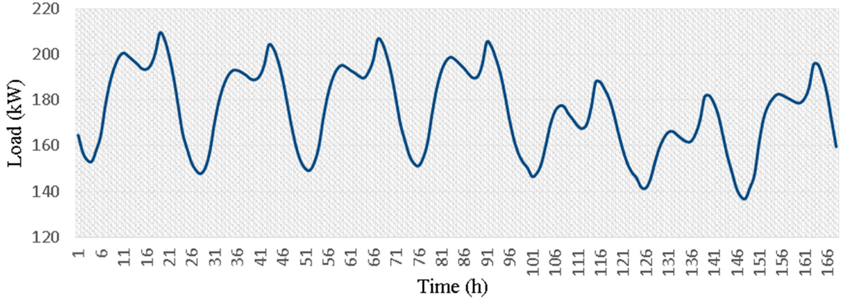
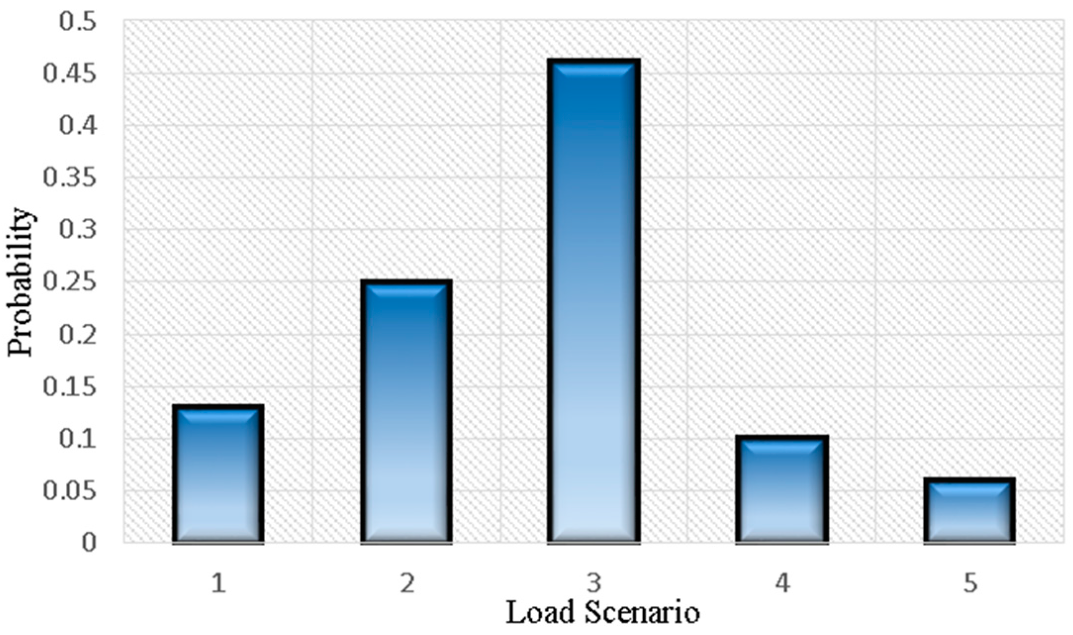
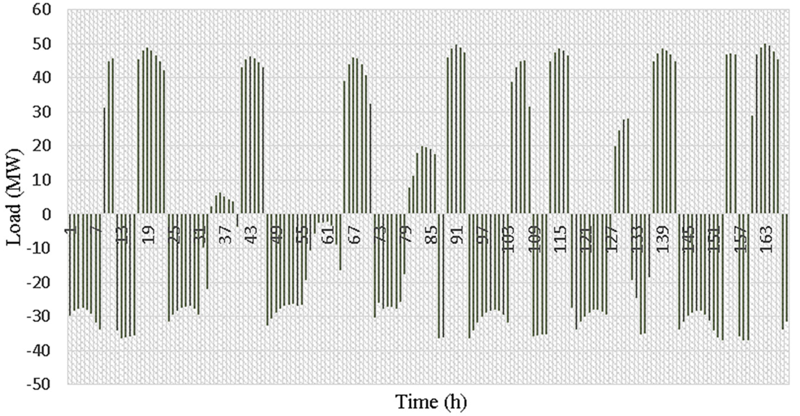
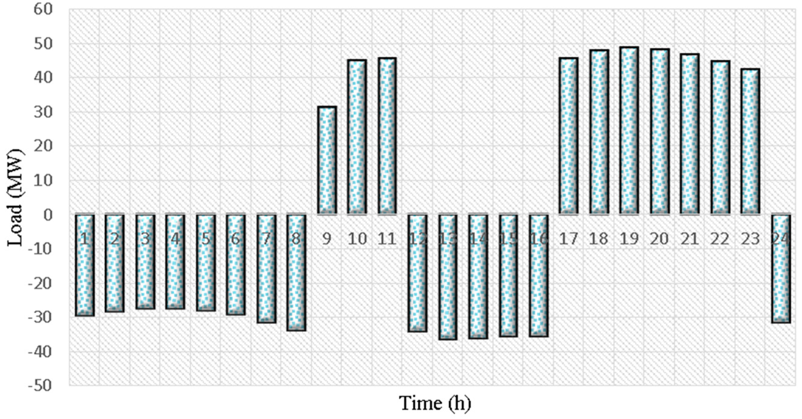
The price data of the spot electricity market is extracted from the New York electricity market data from 2009 to 2015 [47]. The simulation time horizon is 168 hourly time units corresponding to one week. To model the uncertainty of the spot market prices, 10 price scenarios are considered for the study period. Figure 2 illustrates the hourly price profile of the spot market as the average price of the 10 price scenarios considered in this study.

3.1.2. Load Data

The electricity consumption data corresponding to the retailer’s clients is also extracted from the New York electricity market data during 2009–2015 [47]. In this case study, it is assumed that the retailer has retail contracts with only 10 customers and for each customer 5 load scenarios are considered. Figure 3 depicts the total electricity consumption of the retailer’s customers during the one-week scheduling period. The probability distribution of the load scenarios is presented in Figure 4.

We consider a 0.9 lagging power factor for the electrical loads of the network. This assumption is made based on the fact that we focus on the small electricity users, mainly residential loads, and the largest share of the home appliances are inductive loads.

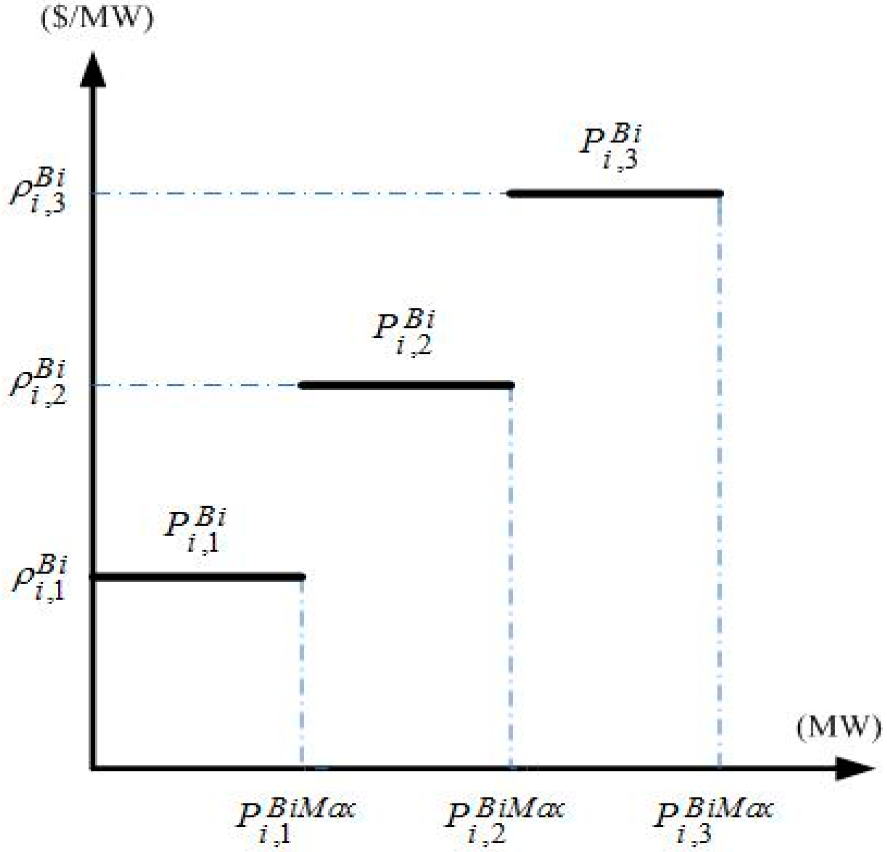
3.1.3. Distributed Generators’ Data

It is assumed that there are five DGs connected to the distributed network from which the retailer can provide electricity. Technical limits of these DG units are presented in

Table 1. Technical limits of the distributed generator (DG) units.

DGs	Min Uptime (h)	Min Down Time (h)	Pmax (MW)	Pmin (MW)
DG 1	1	1	15	0
DG 2	1	1	25	4
DG 3	1	1	30	10
DG 4	1	1	40	15
DG 5	1	1	25	0

.

It is assumed that price offers of DG units are provided to the retailer as block offers with staircase offer curves. Then, the retailer decides on purchasing electrical energy from these DG units based on their prices. In this case study, we assume that each DG owner submits three different power–price offer blocks to the retailer corresponding to low-load, mid-load, and peak-load periods, respectively. The offer price and quantity of the active power and reactive power of the DG units are extracted form New York electricity market data in [47] and tabulated in

Table 2. Data of DGs’ offered price blocks for active power.

	Peak Load Offered Price ($/kWh)					Mid Load Offered Price ($/kWh)					Low Load Offered Price ($/kWh)
Blocks	B 1	B 2	B 3	B 4	B 5	B 1	B 2	B 3	B 4	B 5	B 1	B 2	B 3	B 4	B 5
DG 1	9.3	18.7	26.15	29.33	36.27	3.25	7	13.25	18.42	21.18	2.83	6.57	9.80	11.16	16.72
DG 2	6.73	12.43	14.95	21.51	25.77	3.5	4.85	9.47	10.64	15.41	4.41	8.18	15.38	16.05	18.86
DG 3	9.83	15.52	19.38	20.3	22.63	2.45	7.15	13	13.54	15.82	2.40	2.24	6.94	8.34	12.45
DG 4	5.53	9.11	12.77	17.68	19.92	1.65	4.02	7.3	9.31	14.62	1.19	3.49	7.04	7.59	9.16
DG 5	5	10.04	11.36	13.98	18.33	1.45	3.84	7.54	8.11	9.74	2.68	6.52	9.51	11.34	15.41

,

Table 3. Data of DGs’ offered active power blocks.

	Peak Load Offered Power (kWh)					Mid Load Offered Power (kWh)					Low Load Offered Power (kWh)
Blocks	B 1	B 2	B 3	B 4	B 5	B 1	B 2	B 3	B 4	B 5	B 1	B 2	B 3	B 4	B 5
DG 1	3	4	4	2	2	3	4	4	2	2	5	6	2	1	1
DG 2	4	3	6	7	5	5	5	5	5	5	8	6	3	5	3
DG 3	10	3	5	5	7	12	4	8	2	4	15	8	5	1	1
DG 4	15	5	3	8	9	15	5	8	5	7	15	8	8	5	4
DG 5	3	3	5	6	8	5	4	6	3	7	9	8	6	1	1

,

Table 4. Data of DGs’ offered price blocks for reactive power.

	Peak Load Offered Price ($/KVArh)					Mid Load Offered Price ($/KVArh)					Low Load Offered Price ($/KVArh)
Blocks	B 1	B 2	B 3	B 4	B 5	B 1	B 2	B 3	B 4	B 5	B 1	B 2	B 3	B 4	B 5
DG 1	0.33	0.67	0.93	1.05	1.13	0.10	0.22	0.41	0.58	0.66	0.12	0.15	0.25	0.28	0.42
DG 2	0.24	0.44	0.53	0.77	0.81	0.11	0.15	0.30	0.33	0.48	0.10	0.18	0.39	0.40	0.47
DG 3	0.35	0.55	0.69	0.63	0.71	0.18	0.22	0.41	0.37	0.44	0.11	0.13	0.15	0.18	0.31
DG 4	0.20	0.28	0.40	0.55	0.62	0.15	0.19	0.23	0.29	0.40	0.13	0.15	0.16	0.17	0.22
DG 5	0.18	0.36	0.36	0.44	0.57	0.15	0.17	0.24	0.25	0.27	0.12	0.14	0.21	0.28	0.38

and

Table 5. Data of DGs’ offered reactive power blocks.

	Peak Load Offered Power (KVArh)					Mid Load Offered Power (KVArh)					Low Load Offered Power (KVArh)
Blocks	B 1	B 2	B 3	B 4	B 5	B 1	B 2	B 3	B 4	B 5	B 1	B 2	B 3	B 4	B 5
DG 1	2	2	2	1	1	1.5	2	2	1	1	3	3.5	1	0.5	0.5
DG 2	2	1.5	3	4	2	3	2	2	2	2	4.5	2.5	1.5	2	1.5
DG 3	5	2	2	2	3	7	2	6	1	2	8	4	2	1	0.5
DG 4	10	2	1	3	4	10	2	3	2	4	9	4	4	2	2.5
DG 5	1.5	1	2	3	5	2	1.5	2	2	3	5	4	3.5	0.5	0.5

.

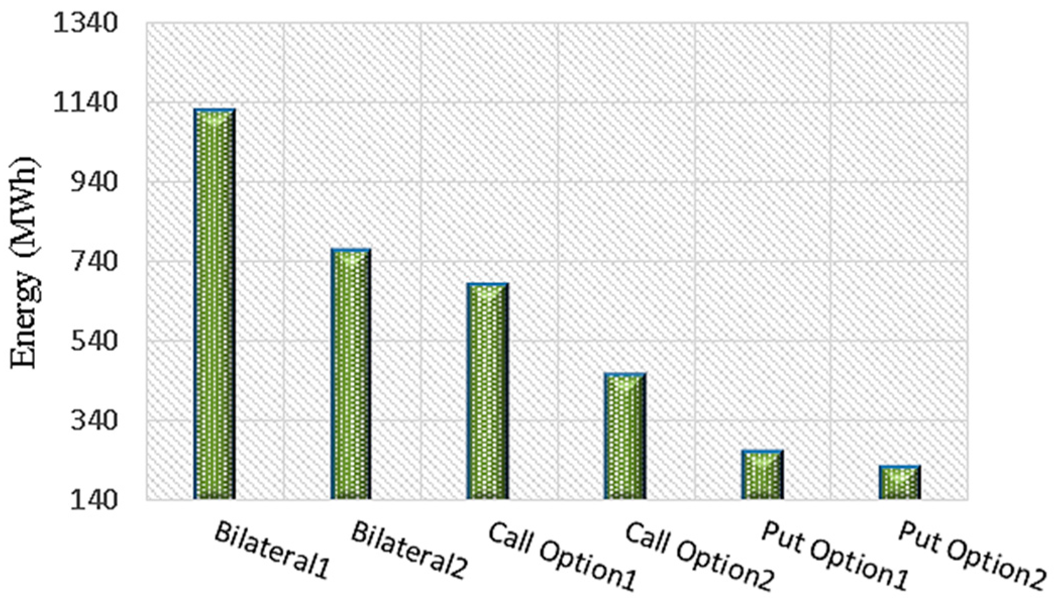
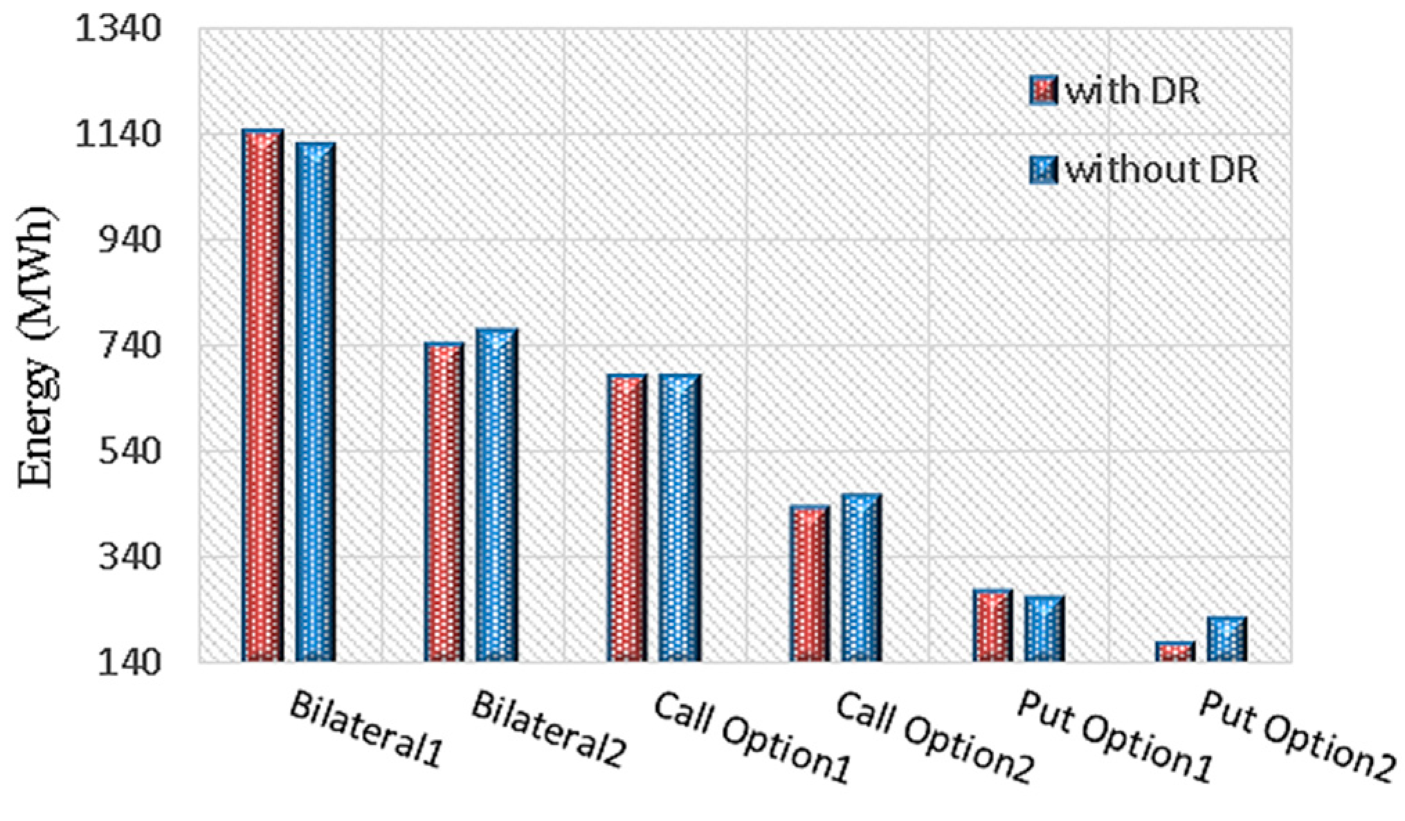
3.1.4. Contracts’ Data

The contracts’ data include contract type, contracted power quantity, number of steps, and operation time horizon of each forward contract. In this study, six contracts from three different contract type, i.e., bilateral contracts, call options, and put options, are considered. The data of these contracts are presented in

Table 6. Contracts’ general data.

Contracts	Prepayment ($/MW)	Minimum Power (MW)	Maximum Power (MW)
Bilateral 1	0	1.5	12
Bilateral 2	0	0.5	10
Call option 1	25	0	8
Call option 2	30	0	9
Put option 1	10	0.25	5
Put option 2	12	0.2	6

,

Table 7. Data of contracts’ offered price steps.

	Peak Load Price			Mid Load Price			Low Load Price
	($/kWh)			($/kWh)			($/kWh)
Step	S 1	S 2	S 3	S 1	S 2	S 3	S 1	S 2	S 3
Bilateral 1	62	81	106	50	75	95	80	95	125
Bilateral 2	68	106	146	56	80	102	88	116	150
Call option 1	80	82.5	85	80	82.5	85	95	115	143
Call option 2	112	126	151	90	95	100	120	145	169
Put option 1	110	125	136	90	105	115	115	120	140
Put option 2	124	139	156	110	132	140	124	139	156

and

Table 8. Data of contracts’ offered power steps.

	Peak Load Power			Mid Load Power			Low Load Power
	(kWh)			(kWh)			(kWh)
Step	S 1	S 2	S 3	S 1	S 2	S 3	S 1	S 2	S 3
Bilateral 1	3	4	5	4	4	4	3	2	7
Bilateral 2	3	3	4	3.3	3.3	3.4	3	4	3
Call option 1	1	3	4	2	2	4	2	3	2
Call option 2	2	2	5	3	3	3	2	4	3
Put option 1	1	2	2	2	1	2	0	3	2
Put option 2	2	2	2	2	1	3	1	3	2

. Without loss of generality, we consider three steps for each contract with different offered power and price for each step. Moreover, similar to the DGs’ offers, it is assumed that each contract consists of three price/quantity offer steps corresponding to the low-load, mid-load and peak-load hours of the day. The offer prices and offer power quantity of each step of different contracts are presented in Table 7 and Table 8. The offered price/quantity steps are extracted from [47].

3.1.5. Other Required Input Data

Other supplementary input parameters needed to perform the simulation, including the risk parameter and selling price data of the retailer, are presented in

Table 9. Supplementary input parameter.

Risk aversion factor	${\rho }_{RM}$	0.5
Confidence level	$\beta -CVaR$	95%
Weighting factor	${\delta }_t^{\omega }$	1
Maximum selling price	$\overline{\rho }$	90 ($/MWh)
Average selling price	${\rho }^{AVG}$	63 ($/MWh)
Minimum selling price	$\underset{\_}{\rho }$	54 ($/MWh)
Retailer’s constant costs	$C^{con}$	35,000$

. During the simulation, the retailer’s selling price data may be changed by the authors, with the aim of analyzing the resulted profit of the retailer. As mentioned before, totally 50 uncertainty scenarios are considered for each hour, including 10 spot market price scenarios and five load scenarios. A retailer should purchase electricity through forward contracts or directly from centralized electricity markets and sell it through contracts, usually with constant price, to its customers

3.2. Results and Discussion

In this section, the simulation results on the test case are presented and discussed. As mentioned before, we consider four different schemes for retailer’s decision-making problem. In the followings, the results of these schemes are compared in terms of retailer’s profitability and risk. Finally, the effectiveness of using demand response programs by retailer on its performance is analyzed.

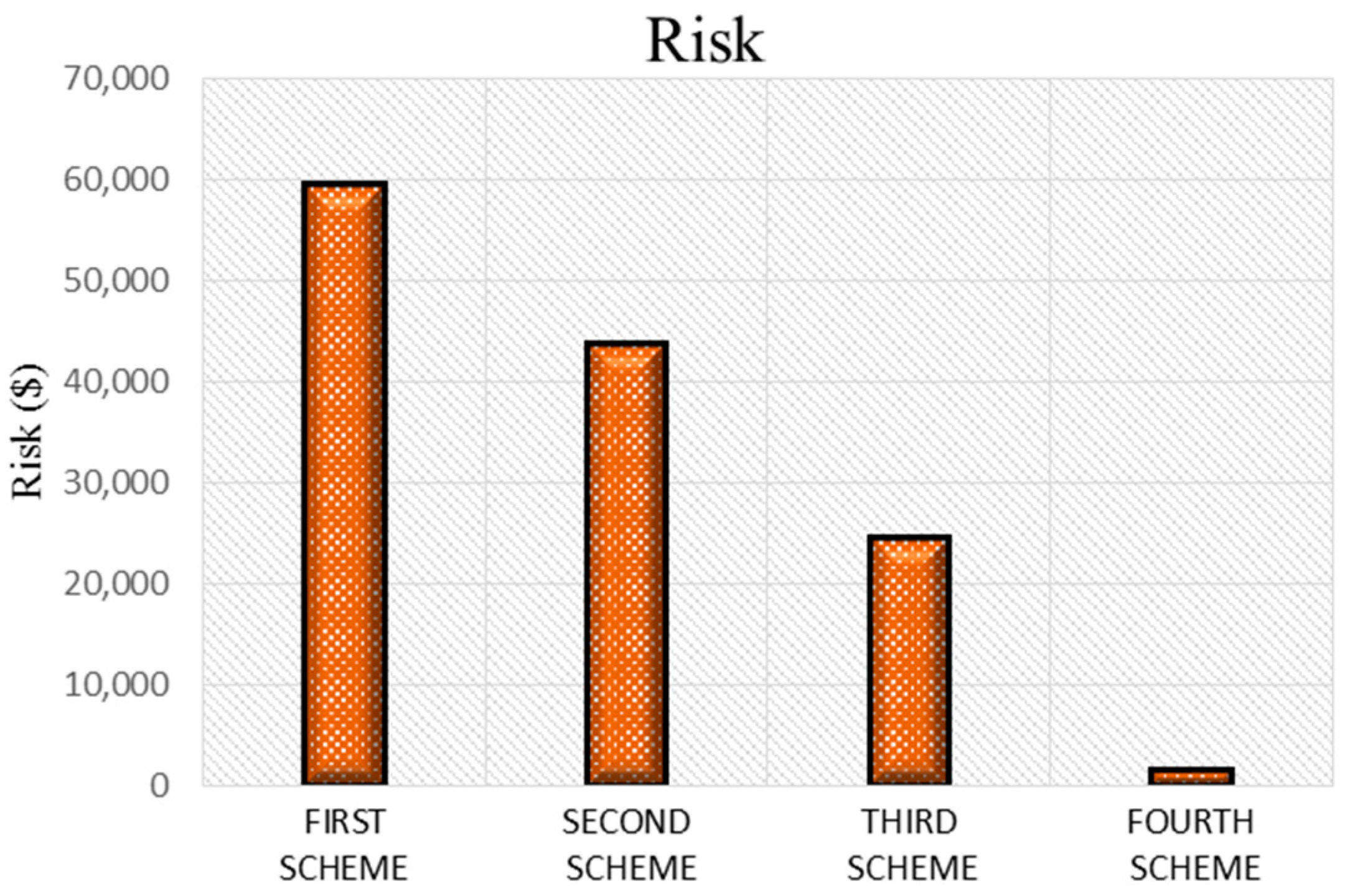
3.2.1. First Scheme: Without Forward Contracts, DGs, and DRP

Under this scheme, the profit of the retailer is −1,287,060$ and its risk is 59,746$ which implies on a highly risky and non-profitable strategy. The retailer needs to buy the whole required energy to supply its customers from the spot electricity market with volatile market prices. Therefore, to remunerate its costs and achieve a positive profit, the retailer needs to increase its selling price to the customers form the values presented in Table 9. Even through selling the electricity with the maximum proposed price (90 $/MWh) to its customers, the retailer cannot reach positive profit in this scheme. Furthermore, one should consider that the retail price increment would in turn decrease the number of retailer’s customers in long term.

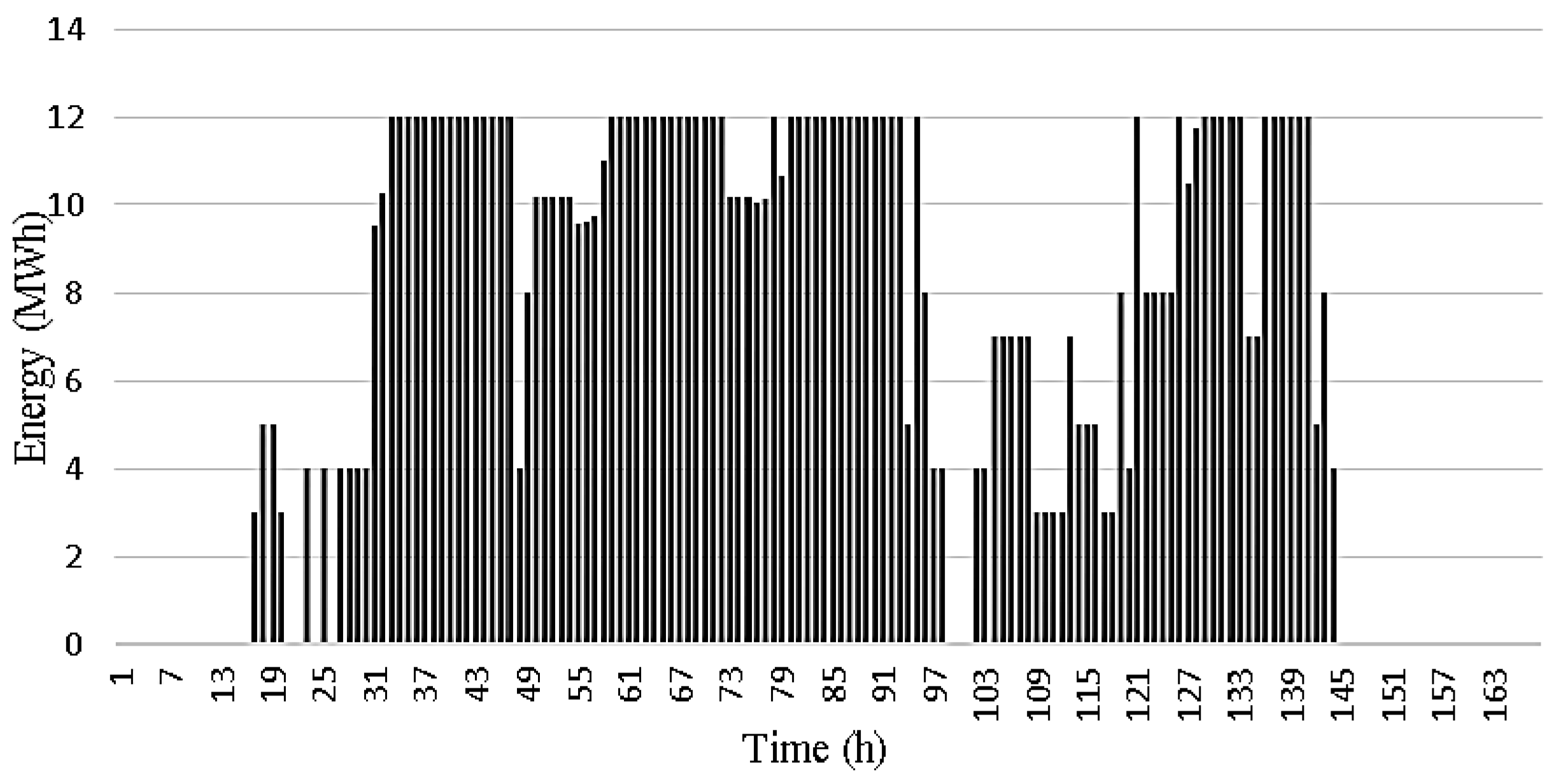
3.2.2. Second Scheme: With DGs but without Forward Contracts and DRP

Under this scheme, the possibility to access distributed generators increases the retailer’s profit to −226,035$ and decreases its risk to 43,912$. However, the retailer still is not able to achieve positive profit without increasing its retail electricity prices. We increase the average selling price of the retailer from the predefined 63 $/MWh is Table 9 in short steps and execute the simulation for each price to achieve a positive profit. Under the average selling price value of 72 $/MWh, the profit becomes positive. Therefore, it is resulted that the retailer needs to increase its average retail prices to minimum 72 $/MWh. The simulation results in terms of retailer’s profit, retailer’s payment to DGs, and retailers’ payment to spot market, under the two average selling prices are presented in

Table 10. Retailer’s profit and costs under different average selling prices in the second scheme.

	For 63 ($/MWh)	For 72 ($/MWh)
Net profit	−226,035	19,236.97
Payment to spot market	1,115,485	1,158,658
Payment to DGs	846,242	849,171.7

.

3.2.3. Third Scheme: With DGs and Forward Contracts but without DRP

Under this scheme, the retailer’s profit is −29,790$ and its risk is 24,638$. Comparing the results to the second scheme, it can be concluded that the ability of the retailer to make forward contracts increases its profit and reduces its risk. However, similar to the previous schemes, the retailer’s profit is negative with 63 $/MWh average selling price. To achieve a positive profit, the retailer needs to increase its average retail price at least 2 $/MWh, to 65 $/MWh. The profit and costs of the retailer under the two average selling prices are presented in

Table 11. Retailer’s profit and costs under different average selling prices in the third scheme.

	For 63($/MWh)	For 65($/MWh)
Net profit	−29,790	11,630
Payment to spot market	626,425	596,420
Payment to DGs	791,614	792,744
Payment to contracts	347,442	370,194

. It can also be concluded that the possibility to make forward contracts enables the retailer to reach profitability with lower risk and lower average selling price which in turn increase its customers’ satisfaction.

Figure 5 illustrates the willingness of the retailer to buy energy from different forward contracts, as introduced in Section 3.1.4. As can be seen in Figure 5, the bilateral contracts tend to be more compelling by the retailer, whereas the put options are the least pleasant contracts.

It should be noted that the structure of the bilateral contracts impacts the strategy of the retailer on buying energy from these contracts during scheduling time horizon. In this example, we considered staircase price curve for the bilateral contracts with3 price steps corresponding to 3 power levels in each period. The energy purchased from the first bilateral contract (Bilateral 1) is shown in Figure 6. In case the offer curve of the bilateral contacts was 1-level instead of 3-level, which means that the price was the same for different energy levels, the energy purchased curve in Figure 6 would have only two levels meaning that the energy was either purchased from the producer or not.

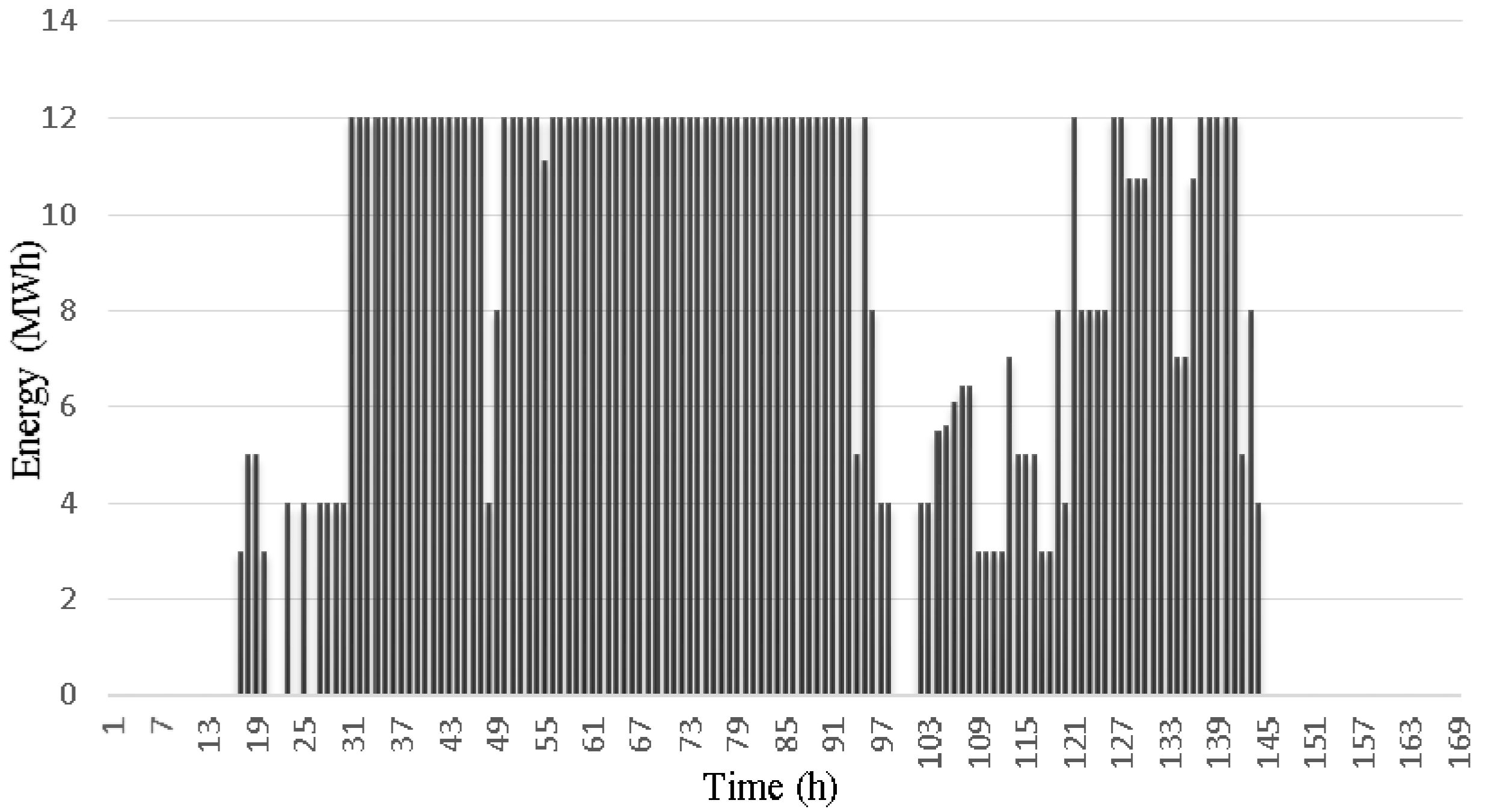
3.2.4. Fourth Scheme: With DGs, forward Contracts, and DRP

Under the assumption of the retailer’s accessibility to DGs, forward contracts, and DRP, the retailer achieves 94,043$ profit and 1548$ risk. Comparing the retailer’s profit to the previous schemes, it can be concluded that only through implementing demand response program the retailer can achieve positive profit with the average selling price of 63 $/MWh, as the input parameter in Table 9. Furthermore, thanks to the DRP, the retailer can decrease its risk up to 93.7% compared to the third scheme. From the customers point of view also this scheme is more preferable, since the retailer can offer the lower retail electricity prices to its customers, without threatening its profitability. Our simulation results indicates that the retailer can decrease its average daily retail prices up to 60 $/MWh during the scheduling horizon under this scheme while keeping its profit positive.

Table 12. Retailer’s profit and costs under different average selling prices in the fourth scheme.

	For 60 ($/MWh)	For 63 ($/MWh)
Net profit	238	94,043
Payment to spot market	566,805	612,408
Payment to DGs	717,642	699,785
Payment to contracts	348,357	329,780

presents the retailer’s profit and payments under the two average retail prices of 63 $/MWh and 60 $/MWh. Compared to the previous schemes, in this scheme the energy purchased from spot market by the retailer decreases which in turn reduces the retailer’s risk.

The willingness of the retailer to provide energy from different forward contracts under the fourth scheme (with and without DRP) is shown in Figure 7. The results indicate that with or without the possibility to implement demand response programs, it is more beneficial for the retailer to buy energy from bilateral contracts. The energy purchased from the first bilateral contract (Bilateral 1) is depicted in Figure 8.

The most remarkable impact which is expected from implementing DRP along with the dynamic pricing approach is to shift electrical load from peak-load hours to mid-load and low-load hours. The load shifting impact of DRP in our case study, during the 1-week scheduling horizon and a sample 24-h horizon are shown in Figure 9 and Figure 10, respectively. The figures show the difference between the electricity demand level and the actual electricity consumption per hour. As can be seen in Figure 10, in the first hour of the sample day, the customers consume almost 30 MW more than the expected demand, whereas during the 10th hour they decrease their consumption up to 45 MW compared to the expected demand. The customers’ load shifting in turn enables the retailer to reduce its risk, as well as the retail average electricity price, compared to the other schemes and simultaneously increase its profit.

In general, decreasing the electricity demand during the peak-load hours by the customers and shifting this demand to the other hours of the day, as shown in Figure 9 and Figure 10, helps the retailer to achieve its main objective, i.e., to decrease its risk and increase its profit. In other words, under this situation, the retailer can provide the total electrical energy demand of its customers with lower cost and gain more profit.

Retailer’ profit and its risk under different schemes are represented in Figure 11 and Figure 12, respectively. These figures provide a comprehensive and comparative view on the results obtained from the previous schemes, in order to analyze the impact of forward contracts, DGs, and DRP on the retailer’s profit and risk. Figure 11 confirms that only through performing DRP, the retailer can achieve positive profit with the average selling price of 63 $/MWh. By comparing four schemes in Figure 12, it can be concluded that by applying DRP the retailer can also decrease its risk to the lowest value compared to the previous schemes.

It should be noted that the presented simulation results are dependent to the assumed offer price of the forward contracts and DGs. In case the offer prices from forward contracts and DGs increases, the retailer may decrease the power purchased form these sources and buy more power from the spot electricity market. On the contrary, if the offer prices of the forward contracts and DG units decrease and their offered power increase, the retailer would provide higher share of its customers’ electrical demand from these sources and reduce its average selling price to the customers.

4. Conclusions

In this paper, the decision-making problem of the retailers under dynamic pricing approach for demand response integration have been investigated. The retailer was supposed to rely on forward contracts, DGs, and spot electricity market to supply the required active and reactive power of its customers. To verify the effectiveness of the proposed model, four schemes for retailer’s scheduling problem are considered and the resulted profit under each scheme are analyzed and compared. The simulation results on a test case indicate that providing more options for the retailer to buy the required power of its customers and increase its flexibility in buying energy from spot electricity market reduces the retailers’ risk and increases its profit. From the customers’ perspective also the retailers’ access to different power supply sources may lead to a reduction in the retail electricity prices. Since the retailer would be able to decrease its electricity selling price to the customers without losing its profitability, with the aim of attracting more customers.

In this work, the conditional value at risk (CVaR) measure is used for considering and quantifying risk in the decision-making problems. Among all the possible option in front of the retailer to optimize its profit and risk, demand response programs are the most beneficial option for both retailer and its customers. The simulation results on the case study prove that implementing dynamic pricing approach on retail electricity prices to integrate demand response programs can successfully provoke customers to shift their flexible demand from peak-load hours to mid-load and low-load hours. Comparing the simulation results of the third and fourth schemes evidences the impact of DRPs and customers’ load shifting on the reduction of retailer’s risk, as well as the reduction of retailer’s payment to contract holders, DG owners, and spot electricity market. Furthermore, the numerical results imply on the potential of reducing average retail prices up to 8%, under demand response activation. Consequently, it provides a win–win solution for both retailer and its customers.

References

1. Kirschen, D.S.; Strbac, G. Fundamentals of Power System Economics; John Wiley & Sons: New York, NY, USA, 2004. [Google Scholar]
2. Nojavan, S.; Zare, K.; Mohammadi-Ivatloo, B. Risk-based framework for supplying electricity from renewable generation-owning retailers to price-sensitive customers using information gap decision theory. Int. J. Electr. Power Energy Syst. 2017, 93, 156–170. [Google Scholar] [CrossRef]
3. Carrion, M.; Conejo, A.J.; Arroyo, J.M. Forward contracting and selling price determination for a retailer. IEEE Trans. Power Syst. 2007, 22, 2105–2114. [Google Scholar] [CrossRef]
4. Shahidehpour, M.; Yamin, H.; Li, Z. Market Overview in Electric Power Systems. Market Operations in Electric Power Systems: Forecasting, Scheduling, and Risk Management; John Wiley & Sons: New York, NY, USA, 2002; pp. 1–20. [Google Scholar]
5. Gabash, A.; Li, P.U. Reverse active-reactive optimal power flow in ADNs: Technical and economical aspects. In Proceedings of the 2014 IEEE International Energy Conference (ENERGYCON), Dubrovnik, Croatia, 13–16 May 2014. [Google Scholar]
6. Gabash, A.; Li, P.U. On variable reverse power flow-part I: Active-Reactive optimal power flow with reactive power of wind stations. Energies 2016, 9, 121. [Google Scholar] [CrossRef]
7. Gabash, A.; Li, P.U. Variable reverse power flow-part II: Electricity market model and results. In Proceedings of the 2015 IEEE 15th International Conference on Environment and Electrical Engineering (EEEIC), Rome, Italy, 10–13 June 2015. [Google Scholar]
8. Gabash, A.; Li, P.U. Active-reactive optimal power flow for low-voltage networks with photovoltaic distributed generation. In Proceedings of the 2012 IEEE International Energy Conference and Exhibition (ENERGYCON), Florence, Italy, 9–12 September 2012. [Google Scholar]
9. Gabash, A.; Li, P.U. Active-reactive optimal power flow in distribution networks with embedded generation and battery storage. IEEE Trans. Power Syst. 2012, 27, 2026–2035. [Google Scholar] [CrossRef]
10. Gabash, A.; Li, P.U. Flexible optimal operation of battery storage systems for energy supply networks. IEEE Trans. Power Syst. 2013, 28, 2788–2797. [Google Scholar] [CrossRef]
11. Kirzner, I.M. Competition and Entrepreneurship; University of Chicago Press: Chicago, IL, USA, 2015. [Google Scholar]
12. Kirzner, I.M. Entrepreneurial discovery and the competitive market process: An Austrian approach. J. Econ. Lit. 1997, 35, 60–85. [Google Scholar]
13. Khojasteh, M.; Jadid, S. Decision-making framework for supplying electricity from distributed generation-owning retailers to price-sensitive customers. Util. Policy 2015, 37, 1–12. [Google Scholar] [CrossRef]
14. Kirschen, D.S. Demand-side view of electricity markets. IEEE Trans. Power Syst. 2003, 18, 520–527. [Google Scholar] [CrossRef]
15. Marzband, M.; Fouladfar, M.H.; Akorede, M.F.; Lightbody, G.; Pouresmaeil, E. Framework for smart transactive energy in home-microgrids considering coalition formation and demand side management. Sustain. Cities Soc. 2018, 40, 136–154. [Google Scholar] [CrossRef]
16. Nojavan, S.; Zare, K.; Mohammadi-Ivatloo, B. Optimal stochastic energy management of retailer based on selling price determination under smart grid environment in the presence of demand response program. Appl. Energy 2017, 187, 449–464. [Google Scholar] [CrossRef]
17. Ayón, X.; Moreno, M.Á.; Usaola, J. Aggregators’ Optimal Bidding Strategy in Sequential Day-Ahead and Intraday Electricity Spot Markets. Energies 2017, 10, 450. [Google Scholar] [CrossRef]
18. Eydeland, A.; Wolyniec, K. Energy and Power Risk Management: New Developments in Modeling, Pricing, and Hedging; John Wiley & Sons: New York, NY, USA, 2003; Volume 206. [Google Scholar]
19. Sheikhahmadi, P.; Mafakheri, R.; Bahramara, S.; Damavandi, M.Y.; Catalão, J.P. Risk-Based Two-Stage Stochastic Optimization Problem of Micro-Grid Operation with Renewables and Incentive-Based Demand Response Programs. Energies 2018, 11, 610. [Google Scholar] [CrossRef]
20. Li, Y.-P.; Li, X.-G. Power supplier’s risk types and optimal asset management reckon in biding failure. In Proceedings of the Third International Conference on Electric Utility Deregulation and Restructuring and Power Technologies, Nanjing, China, 6–9 April 2008; pp. 557–560. [Google Scholar]
21. Yu, Q.; Zhang, L. Research in bidding strategies under different price mechanisms in generation-right trading. In Proceedings of the 2011 2nd International Conference on Artificial Intelligence, Management Science and Electronic Commerce (AIMSEC), Zhengzhou, China, 8–10 August 2011; pp. 4197–4200. [Google Scholar]
22. Hatami, A.; Seifi, H.; Sheikh-El-Eslami, M.K. A stochastic-based decision-making framework for an electricity retailer: Time-of-use pricing and electricity portfolio optimization. IEEE Trans. Power Syst. 2011, 26, 1808–1816. [Google Scholar] [CrossRef]
23. Tavakoli, M.; Shokridehaki, F.; Akorede, M.F.; Marzband, M.; Vechiu, I.; Pouresmaeil, E. CVaR-based energy management scheme for optimal resilience and operational cost in commercial building microgrids. Int. J. Electr. Power Energy Syst. 2018, 100, 1–9. [Google Scholar] [CrossRef]
24. Tanlapco, E.; Lawarrée, J.; Liu, C.-C. Hedging with futures contracts in a deregulated electricity industry. IEEE Trans. Power Syst. 2002, 17, 577–582. [Google Scholar] [CrossRef]
25. Imani, M.H.; Niknejad, P.; Barzegaran, M. The impact of customers’ participation level and various incentive values on implementing emergency demand response program in microgrid operation. Int. J. Electr. Power Energy Syst. 2018, 96, 114–125. [Google Scholar] [CrossRef]
26. Act, E.P. Energy Policy Act of 2005; US Congress: Washington, DC, USA, 2005.
27. Valero, S.; Ortiz, M.; Senabre, C.; Alvarez, C.; Franco, F.; Gabaldon, A. Methods for customer and demand response policies selection in new electricity markets. IET Gener. Transm. Distrib. 2007, 1, 104–110. [Google Scholar] [CrossRef]
28. Ma, Z.; Billanes, J.D.; Jørgensen, B.N. Aggregation Potentials for Buildings—Business Models of Demand Response and Virtual Power Plants. Energies 2017, 10, 1646. [Google Scholar]
29. Abrishambaf, O.; Ghazvini, M.A.F.; Gomes, L.; Faria, P.; Vale, Z.; Corchado, J.M. Application of a home energy management system for incentive-based demand response program implementation. In Proceedings of the 2016 27th International Workshop on Database and Expert Systems Applications (DEXA), Porto, Portugal, 5–8 September 2016; pp. 153–157. [Google Scholar]
30. Yousefi, S.; Moghaddam, M.P.; Majd, V.J. Optimal real time pricing in an agent-based retail market using a comprehensive demand response model. Energy 2011, 36, 5716–5727. [Google Scholar] [CrossRef]
31. Nwulu, N.I.; Xia, X. Optimal dispatch for a microgrid incorporating renewables and demand response. Renew. Energy 2017, 101, 16–28. [Google Scholar] [CrossRef]
32. Zhang, C.; Xu, Y.; Dong, Z.Y.; Wong, K.P. Robust coordination of distributed generation and price-based demand response in microgrids. IEEE Trans. Smart Grid 2017. [Google Scholar] [CrossRef]
33. Bompard, E.; Ma, Y.; Napoli, R.; Abrate, G. The demand elasticity impacts on the strategic bidding behavior of the electricity producers. IEEE Trans. Power Syst. 2007, 22, 188–197. [Google Scholar] [CrossRef]
34. Aghaei, J.; Alizadeh, M.-I.; Siano, P.; Heidari, A. Contribution of emergency demand response programs in power system reliability. Energy 2016, 103, 688–696. [Google Scholar] [CrossRef]
35. Nguyen, D.T.; Negnevitsky, M.; De Groot, M. Pool-based demand response exchange—Concept and modeling. IEEE Trans. Power Syst. 2011, 26, 1677–1685. [Google Scholar] [CrossRef]
36. Marzband, M.; Azarinejadian, F.; Savaghebi, M.; Pouresmaeil, E.; Guerrero, J.M.; Lightbody, G. Smart transactive energy framework in grid-connected multiple home microgrids under independent and coalition operations. Renew. Energy 2018, 126, 95–106. [Google Scholar] [CrossRef]
37. Wei, W.; Liu, F.; Mei, S. Energy pricing and dispatch for smart grid retailers under demand response and market price uncertainty. IEEE Trans. Smart Grid 2015, 6, 1364–1374. [Google Scholar] [CrossRef]
38. Mahmoudi, N.; Eghbal, M.; Saha, T.K. Employing demand response in energy procurement plans of electricity retailers. Int. J. Electr. Power Energy Syst. 2014, 63, 455–460. [Google Scholar] [CrossRef]
39. Dutta, G.; Mitra, K. A literature review on dynamic pricing of electricity. J. Oper. Res. Soc. 2017, 68, 1131–1145. [Google Scholar] [CrossRef]
40. Karandikar, R.; Khaparde, S.; Kulkarni, S. Strategic evaluation of bilateral contract for electricity retailer in restructured power market. Int. J. Electr. Power Energy Syst. 2010, 32, 457–463. [Google Scholar] [CrossRef]
41. Fotouhi Ghazvini, M.A.; Soares, J.; Morais, H.; Castro, R.; Vale, Z. Dynamic Pricing for Demand Response Considering Market Price Uncertainty. Energies 2017, 10, 1245. [Google Scholar] [CrossRef]
42. Sheybani, H.R.; Buygi, M.O. Put Option Pricing and Its Effects on Day-Ahead Electricity Markets. IEEE Syst. J. 2017. [Google Scholar] [CrossRef]
43. Barroso, L.A.; Rosenblatt, J.; Guimarães, A.; Bezerra, B.; Pereira, M.V. Auctions of contracts and energy call options to ensure supply adequacy in the second stage of the Brazilian power sector reform. In Proceedings of the 2006 IEEE Power Engineering Society General Meeting, Montreal, QC, Canada, 18–22 June 2006. [Google Scholar]
44. Rockafellar, R.T.; Uryasev, S. Conditional value-at-risk for general loss distributions. J. Bank. Financ. 2002, 26, 1443–1471. [Google Scholar] [CrossRef] [Green Version]
45. Valinejad, J.; Marzband, M.; Akorede, M.F.; Barforoshi, T.; Jovanović, M. Generation expansion planning in electricity market considering uncertainty in load demand and presence of strategic GENCOs. Electr. Power Syst. Res. 2017, 15, 92–104. [Google Scholar] [CrossRef]
46. Available online: http://www.gams.com (accessed on 24 April 2018).
47. Available online: http://www.nyiso.com (accessed on 24 April 2018).
Figure 1. Offer curve of bilateral contracts.
Energies 11 01602 g001
Figure 2. Average spot market prices during the scheduling period.
Energies 11 01602 g002
Figure 3. Total electricity consumption of the retailer’s customers during the scheduling period.
Energies 11 01602 g003
Figure 4. Probability distribution of customers’ load scenarios.
Energies 11 01602 g004
Figure 5. Energy provided through different forward contracts in the third scheme.
Energies 11 01602 g005
Figure 6. Energy purchased from the Bilateral 1 contract under the third scheme.
Energies 11 01602 g006
Figure 7. Energy provided through different forward contracts in the fourth scheme.
Energies 11 01602 g007
Figure 8. Energy purchased from the Bilateral 1 contract under the fourth scheme.
Energies 11 01602 g008
Figure 9. Difference between the demand level and the actual electricity consumption over the scheduling time horizon.
Energies 11 01602 g009
Figure 10. Difference between the demand level and the actual electricity consumption over a 24-h time horizon.
Energies 11 01602 g010
Figure 11. Retailer’ profit under different schemes with the average selling price of 63 $/MWh.
Energies 11 01602 g011
Figure 12. Amount of Risk under different scheme with the average selling price of 63 $/MWh.
Energies 11 01602 g012