Low-Frequency Oscillation Suppression of the Vehicle–Grid System in High-Speed Railways Based on H∞ Control

Abstract

Recently, a traction blockade in the depots of numerous electric multiple units (EMUs) of high-speed railways has occured and resulted in some accidents in train operation. The traction blockade is caused by the low-frequency oscillation (LFO) of the vehicle–grid (EMUs–traction network) system. To suppress the LFO, a scheme of EMUs line-side converter based on the H∞ control is proposed in this paper. First, the mathematical model of the four-quadrant converter in EMUs is presented. Second, the state variables are determined and the weighting functions are selected. Then, an H∞ controller based on the dq coordinate is designed. Moreover, compared with the simulation results of traditional proportional integral (PI) control, auto-disturbance rejection control (ADRC) and multivariable control (MC) based on Matlab/Simulink and the RT-LAB platform, the simulation results of the proposed H∞ control confirm that the H∞ controller applied in EMUs of China Railway High-Speed 3 has better dynamic and static performances. Finally, a whole cascade system model of EMUs and a traction network is built, in which a reduced-order model of a traction network is adopted. The experimental results of multi-EMUs accessed in the traction network indicate that the H∞ controller has good suppression performance for the LFO of the vehicle–grid system. In addition, through the analysis of sensitivity of the H∞ controller and the traditional PI controller, it is indicated that the H∞ controller has better robustness.

1. Introduction

With the rapid development of high-speed railways during recent years, plenty of electric multiple units (EMUs) have been put into operation in passenger railways, interurban railways, and high-speed railways in China. Because of the heavy operation of EMUs and electric locomotives, low-frequency voltage oscillation (LFO) problems happened worldwide. During 2009–2014, LFOs happened in the EMUs depots of Zhengzhou, Nanjing, Shenyang, and some other cities in China [1,2,3,4]. And the LFOs cause some severe accidents, which affects EMUs safety and dispatch. The protection logic operation of the line-side converter of EMUs would be triggered due to the larger voltage oscillation amplitude of traction network, which results in traction blockades and makes the EMUs lose traction power [5]. Because of the severe threat to the safety of high-speed railway operation, these problems should be urgently solved.

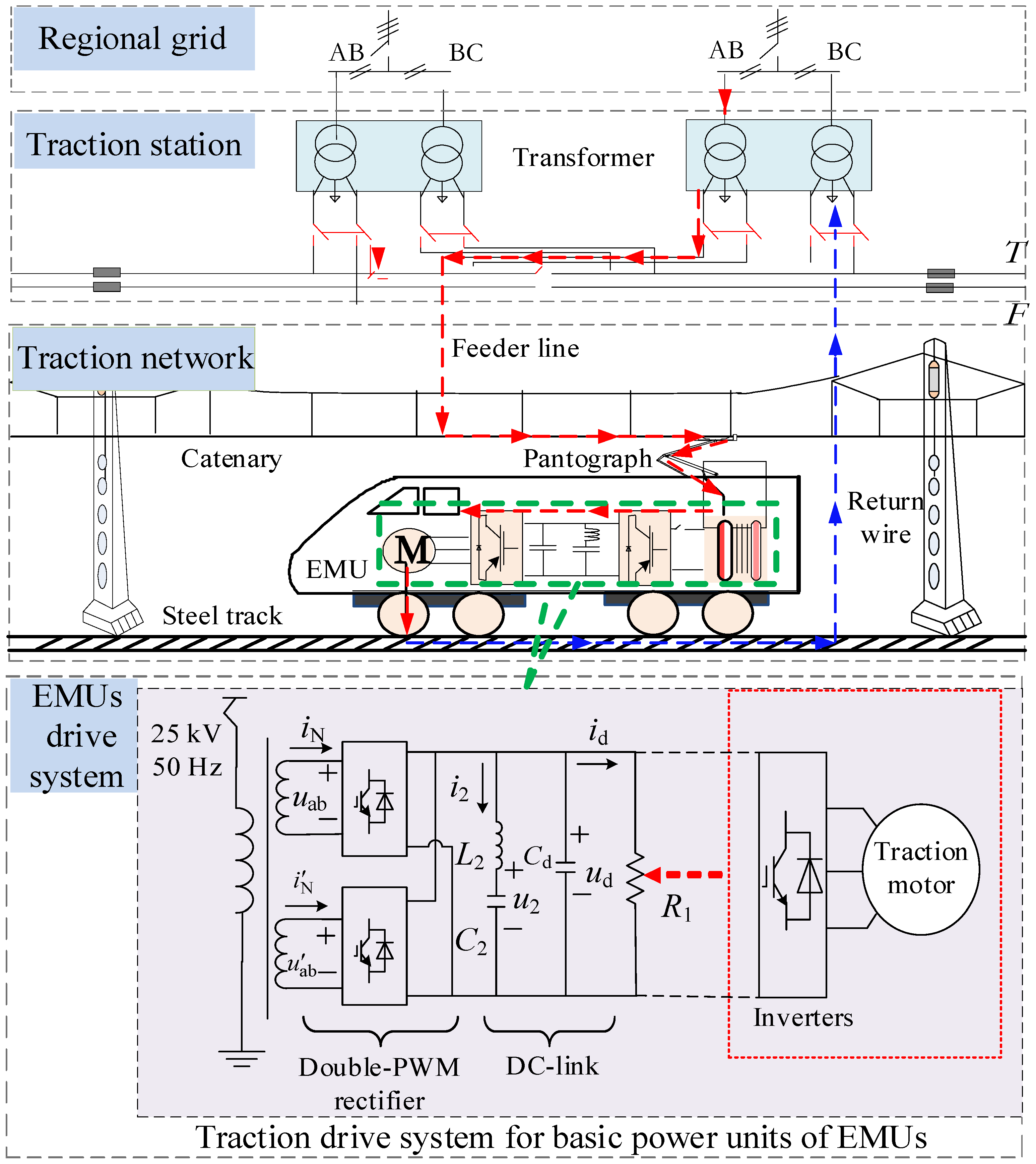
At present, there have been many research studies on LFOs. An LFO usually happens if more than six EMUs are accessed in the auto-transform (AT) station network and at the same time the inverter and motor are basically in an inoperative state. The diagram of a traction network and EMUs is shown in Figure 1. In references [2,3,4,5], it was indicated that LFOs is closely related to the parameters of the line-side converter controllers, especially the parameters of the proportional integral (PI) controller. The implementation of PI controller is simple, and it can make the EMUs–traction network cascade system have the good stability. However, the dynamic performance of the system would become worse when the system is disturbed. The dominant poles triggering LFO were derived based on the dq decomposition method in single-phase system [6]. In [7], the influence of the semiconductor switching on the stability limit of the traction power supply system was studied. In order to analyze the low-frequency instability of locomotives in a railway traction network, the input admittance was measured in [8]. In references [9,10], the derivation of a multivariable control (MC) concept was used to achieve better dynamic performance. The MC is a nonlinear control method, which can transform the nonlinear system into a linear system characterized by the selected state variables.

The LFO problem could be simplified as a dynamic stability problem of large-scale multi-converter system. In the vehicle–grid cascade system, improving the control strategy of the line-side converter of EMUs is usually proposed to ensure stability and suppress LFOs. At present, the traditional linear PI controller is widely used in the line-side converter control of China Railway High-speed (CRH) EMUs. However, it is difficult to adjust PI control parameters, and they are very sensitive to the disturbance of the system. In addition, the line-side converter of EMUs is a typical nonlinear, multi-variable, and strong coupling system, which is sensitive to variations in external disturbance and system parameters. Therefore, it is difficult to achieve the ideal control effect using traditional linear control. In reference [5], auto-disturbance rejection control (ADRC) was adopted to suppress LFOs. The ADRC controller is an improvement to the PI controller, and it eliminates the integration step and adds an extended state observer to realize real-time estimation of the internal model perturbation and external disturbances. But the parameter setting is complex and difficult. H∞ is a control method based on precise mathematical models. During the design process, the uncertainties of system can be considered and a strong anti-interference ability is ensured. When the parameters of the controlled object are changed or the uncertainty disturbance is encountered, it still has a good control effect and strong robustness, and it is not sensitive to the control parameters [11,12,13]. However, it is difficult to select the appropriate weighting functions for the H∞ mixed sensitivity problem [14]. The H∞ mixed sensitivity problem can be attributed to an optimization problem if the weighting functions are considered as variables. However, this optimization has various constraints and it is very complicated. In general, particle swarm optimization (PSO) is an efficient optimization algorithm. PSO will be used to optimize the parameters of weighting functions in this paper.

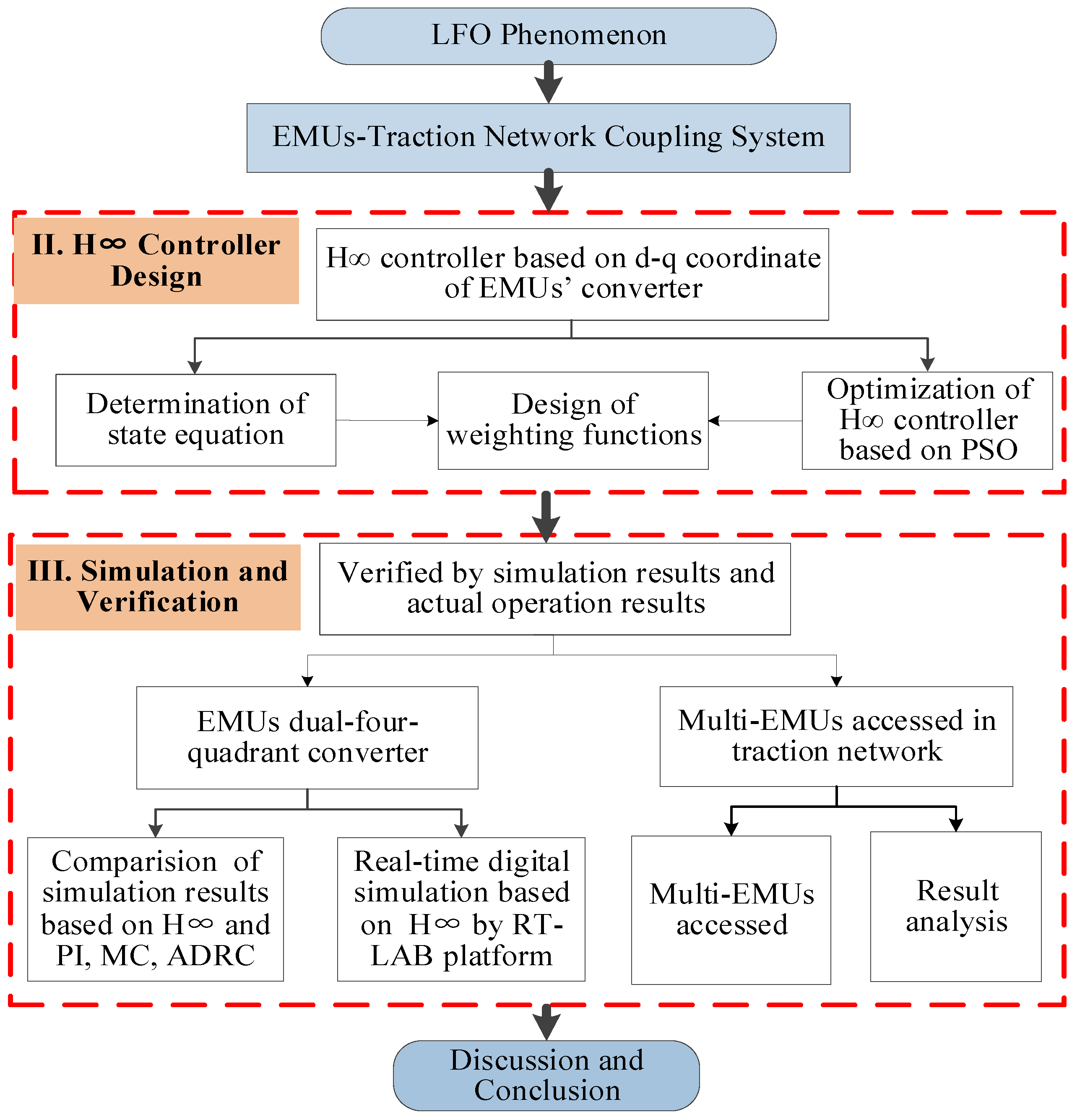
This paper is organized as follows. Section 2 designs the H∞ controller of the line-side converter of EMUs based on a dq coordinate. Section 3 completes the simulations and analysis for a dual line-side converter. Section 4 establishes the reduced-order model of the traction network, and compares the simulations of multi-EMUs accessed in the traction network based on a PI controller and the H∞ controller. Additionally, we indicate that the H∞ controller is not sensitive to high external noise, the model parameters, or the control parameters by comparing the control parameters between the H∞ controller and the PI controller. The LFO suppression strategy based on the H∞ controller is verified. Section 5 gives some conclusions. The whole idea in this paper is described in Figure 2.

2. H∞ Controller Design of the Line-Side Converter of EMUs

2.1. Model Review of the Line-Side Converter of EMUs

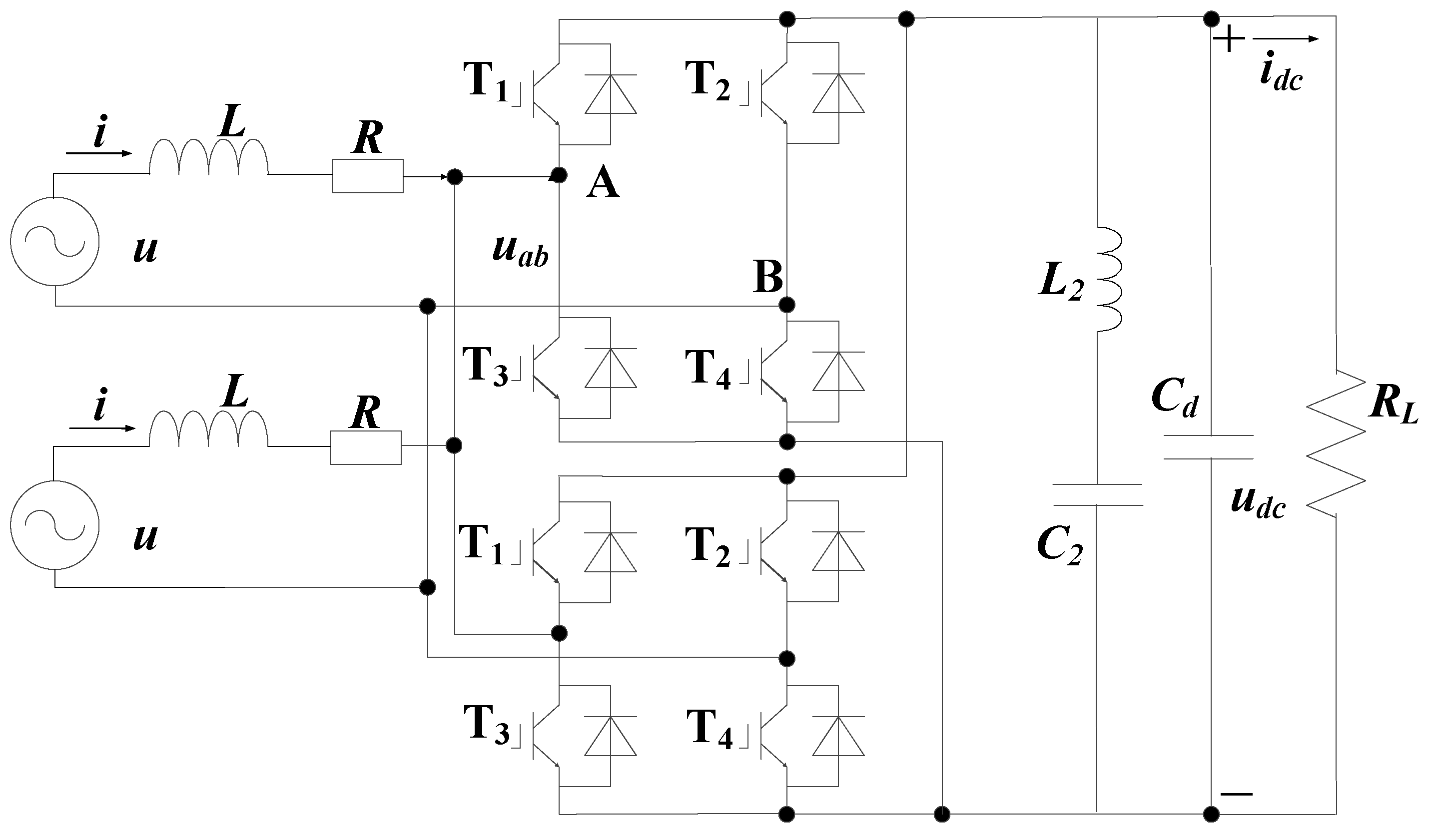
CRH3 EMUs in China adopt dual interleaved pulse-width modulation (PWM) converters, whose equivalent circuit is shown in Figure 3. When the LFO happens, a lot of EMUs are at a standstill and only the auxiliary devices are powered by the DC-link of converters. Therefore, the inverter and traction motor of the vehicle-grid system are simplified to resistance $R_L$ [15]. L and R are the traction winding leakage inductance and resistance, respectively. The $C_d$ is the DC-link capacitor. $L_2$ and $C_2$ are the series resonant circuit inductance and capacitance. T₁, T₂, T₃, and T₄ are the four IGBTs of the two-level converter.

In Figure 3, $u,i$ and $u_{ab}$ are the line voltage, the line current, and the input voltage of the converter, respectively. $u_{dc}$ and $i_{dc}$ are the output voltage and current of the converter, respectively.

The line voltage $u$ and the line current $i$ are defined below.

$$u=U_m\sin \omega t$$

(1)

$$i=I_m\sin (\omega t+\phi )=I_d\sin \omega t+I_q\cos \omega t$$

(2)

where $U_m$ and $I_m$ represent the peak values of the line voltage and line current, respectively. $\omega$ represents the angular frequency of the line voltage, and $\phi$ represents the power factor angle. $i_d$, $i_q$, $u_d$, and $u_q$ represent the DC components of $i$ and $u_{ab}$ in the dq frame, respectively.

The voltage across inductor $L$ yields

$$L\frac{di}{dt}=u-Ri-u_{ab}.$$

(3)

The mathematic model of the line-side converter of EMUs in the dq reference frame in [16] is depicted as follows.

$$\{\begin{array}{l}\frac{d{u}^2{}_{dc}}{dt}=-\frac{2u^2{}_{dc}}{R_L{C}_d}+\frac{u_d{i}_d}{C_d}+\frac{u_q{i}_q}{C_d}\\ L\frac{d{i}_d}{dt}=-R{i}_d+\omega L{i}_q+u_d\\ L\frac{d{i}_q}{dt}=-R{i}_q-\omega L{i}_d+u_q\end{array}$$

(4)

2.2. H∞ Controller State Variable Problem

The core of designing H∞ controller is to find appropriate weighting matrices and an augmented model. The augmented plant equations with the following state-space are introduced below [14].

$$\{\begin{array}{l}\dot{\mathit{x}}=\mathit{A}\mathit{x}+{\mathit{B}}_1\mathit{\epsilon }+{\mathit{B}}_2\mathit{u}\\ \mathit{z}={\mathit{C}}_1\mathit{x}+{\mathit{D}}_{11}\mathit{\epsilon }+{\mathit{D}}_{12}\mathit{u}\\ \mathit{y}={\mathit{C}}_2\mathit{x}+{\mathit{D}}_{21}\mathit{\epsilon }+{\mathit{D}}_{22}\mathit{u}\end{array}$$

(5)

where x(t) represents the plant state vector, u(t) represents the control input, ε(t) represents the external input, which includes plant disturbances and the measurement noise, z(t) represents the regulated output, and y(t) represents the measured output. A, B₁, B₂, C₁, C₂, D₁₁, D₁₂, D₂₁, and D₂₂ represent the constant matrices, and the state variable vector x(t) represents selected below.

$$\left[\begin{array}{l}{x}_1\\ x_2\\ x_3\end{array}\right]=\left[\begin{array}{c}\begin{array}{c}{u}_{dc}\\ \frac{e}{s+K_a}\end{array}\\ \frac{e}{s+K_b}\end{array}\right]$$

(6)

where $e=u_{{}_{dc}}^{*}-u_{dc}$, s represents a differential operator, and $u_{dc}^{{}^{\ast }}$ represents the reference of the DC-link voltage. $K_a$ and $K_b$ represent the underdetermined parameters, and ε(t) is selected as follows.

$$\mathit{\epsilon }=\left[\begin{array}{c}{u}^{\ast }{}_{dc}\\ i\\ n_{noise}\end{array}\right]$$

(7)

where $n_{noise}$ is the measured noise of the DC-link voltage. Additionally, the control input u(t) is selected as

$$\mathit{u}=\left[i^{\ast }{}_d\right]$$

(8)

where $i_d^{*}$ is the reference of $i_d$.

Then, the parameters of matrices in the system state equation can be obtained as follows.

$$\begin{array}{l}\mathit{A}=\left[\begin{array}{ccc}\begin{array}{c}-\frac{1}{R_L{C}_d}\\ -1\\ 1\end{array}& \begin{array}{c}0\\ -K_a\\ 0\end{array}& \begin{array}{c}0\\ 0\\ -K_d\end{array}\end{array}\right]\hspace{1em}\hspace{1em}{\mathit{B}}_1=\left[\begin{array}{ccc}\begin{array}{c}0\\ 1\\ 0\end{array}& \begin{array}{c}-\frac{1}{C_d}\\ 0\\ 0\end{array}& \begin{array}{c}0\\ -1\\ 0\end{array}\end{array}\right]\begin{array}{cc}& {\mathit{B}}_2=\left[\begin{array}{c}\frac{1}{C_d}\\ 0\\ 0\end{array}\right]\end{array}\\ {\mathit{C}}_1=\left[\begin{array}{ccc}\begin{array}{c}-K_b\\ 0\\ K_e\end{array}& \begin{array}{c}{K}_c-K_a{K}_b\\ 0\\ 0\end{array}& \begin{array}{c}0\\ 0\\ K_f-K_d{K}_e\end{array}\end{array}\right]\hspace{1em}\hspace{1em}{\mathit{C}}_2=\left[-1\begin{array}{cc}\begin{array}{cc}& 0\end{array}& 0\end{array}\right]\begin{array}{cc}& {\mathit{D}}_{12}=\left[\begin{array}{c}0\\ K_g\\ 0\end{array}\right]\end{array}\end{array}$$

(9)

where $K_c,K_d,K_e,K_f$, and $K_g$ are the parameters that need to be determined, and D₁₁ = D₂₁ =D₂₂ = 0.

2.3. H∞ Controller Mixed Sensitivity Problem

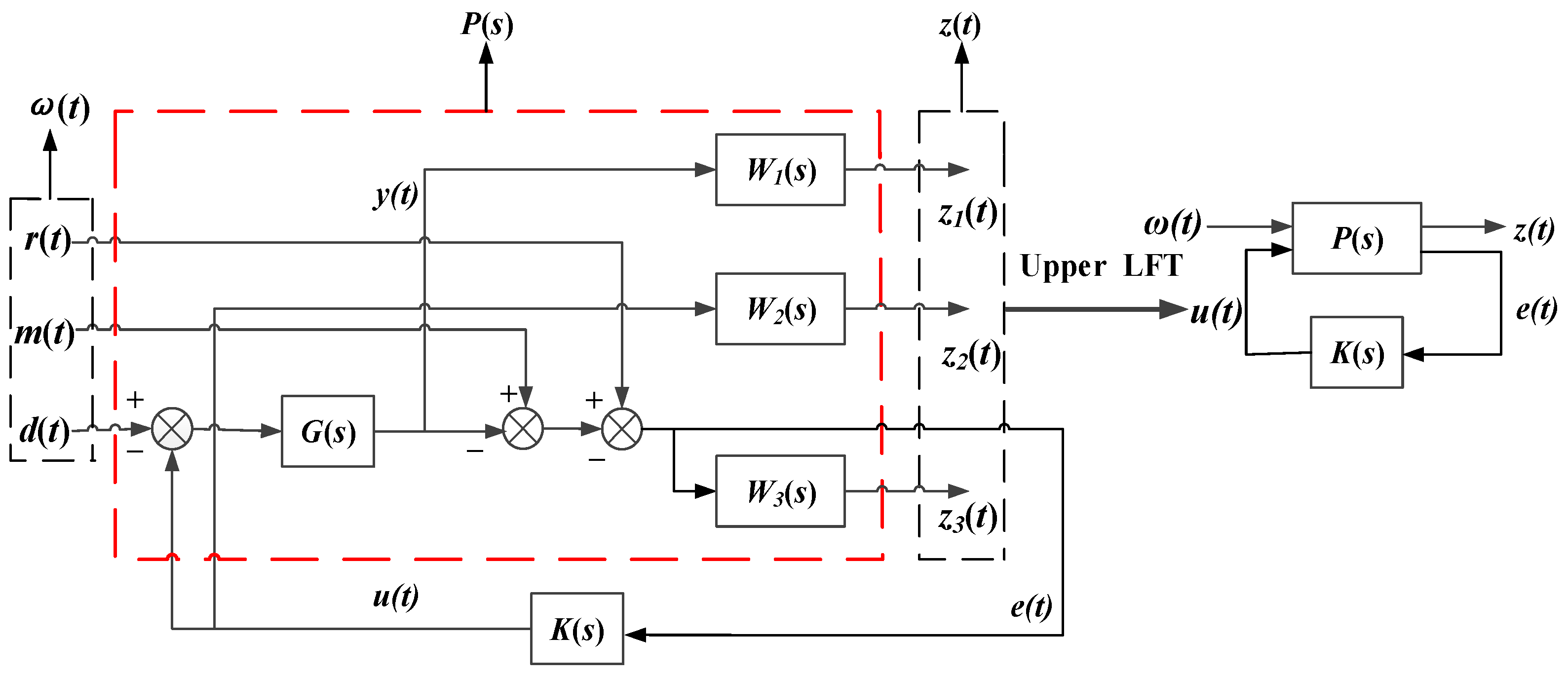
Through the upper linear fractional transformation (LFT), the mixed sensitivity problem can be transformed into the problem of the standard H∞ control [9]. The structures of the mixed-sensitivity problem and the standard H∞ control are shown in Figure 4. P(s), G(s), and K(s) represent the augmented plant, the plant, and the controller, respectively. r(t), m(t), d(t), e(t), u(t), and y(t) represent the reference input signal, the measurement noise signal, the environmental disturbance signal, the tracking error signal, the control input signal, and the system output signal, respectively. z₁(t), z₂(t), and z₃(t) represent the evaluation signals to the weight augmentation system. W₁(s), W₂(s), and W₃(s) represent the performance weighting function, the output limiter weighting function for the controller, and the robust weighting function, respectively.

Given a scalar ${\gamma }_1>0$, the H∞ suboptimal objective is to find a H∞ suboptimal controller that can stabilize the closed loop system ${\mathit{H}}_{z\omega }\left(s\right)$ from $\omega$ to $z$ and satisfy (10) and (11) as

$${\Vert {\mathit{H}}_{z\omega }\left(s\right)\Vert }_{\infty }=\Vert \begin{array}{l}{\mathit{W}}_3\mathit{S}\\ {\mathit{W}}_2\mathit{R}\\ {\mathit{W}}_1\mathit{T}\end{array}\Vert <{\gamma }_1$$

(10)

where S(s) represents the sensitivity matrix function, R(s) represents the enter sensitivity function, and T(s) represents the complementary sensitivity function. These functions can be described as follows.

$$\{\begin{array}{l}\mathit{S}={\left(\mathit{I}+\mathit{G}\mathit{K}\right)}^{-1}\\ \mathit{R}=\mathit{K}{\left(\mathit{I}+\mathit{G}\mathit{K}\right)}^{-1}=\mathit{K}\mathit{S}\\ \mathit{T}=\mathit{G}\mathit{K}{\left(\mathit{I}+\mathit{G}\mathit{K}\right)}^{-1}=\mathit{I}-\mathit{S}\end{array}$$

(11)

where I represents the unit matrix whose order is as same as that of matrix GK.

2.4. Design of Weighting Functions

For the engineering application, it is difficult to give a clear and general formula and choose the H∞ weighting functions due to the existence of various practical problems. The choice of weighting functions depends more on the designer’s experience [17,18]. To track the reference signal and suppress the disturbance, $W_3(s)$ should have the low-pass characteristic with high gain. Because of multiplicative uncertainties of high frequencies, $W_1(s)$ should have a high-pass characteristic. A suitable $W_2(s)$ can provide the enough bandwidth and avoid an overlarge amount of control energy going to the system. Furthermore, the choice of the weighting functions in this paper needs to satisfy the following requirements [11,19].

(1) In order to satisfy the first theorem of robust control, $W_1(s)$ and $W_3(s)$ should meet the following inequality constraint, which will avoid the formation of an overlapping frequency range between $W_1(s)$ and $W_3(s)$:

$$\sigma \left[W_1{}^{-1}(s)\right]+\sigma \left[W_3{}^{-1}(s)\right]\ge 1.$$

(12)

(2) The maximum singular value of the sensitivity function $S(s)$ should be less than the maximum singular value of $W_1^{-1}(s)$ in the whole frequency range.

$$\sigma \left[S(s)\right]<\sigma \left[W_1{}^{-1}(s)\right]$$

(13)

(3) The maximum singular value of the complementary sensitivity function $T(s)$ should be less than the maximum singular value of $W_3{}^{-1}(s)$ in the whole frequency range.

$$\sigma \left[T(s)\right]<\sigma \left[W_3{}^{-1}(s)\right]$$

(14)

To increase the stability of the EMUs–traction network cascade system, the structures of $W_3\left(s\right)$ and $W_1\left(s\right)$ are chosen as a stable first-order continuous time form. The structure of $W_2\left(s\right)$ is chosen as a scalar form. The weighting functions are described as follows.

$$\{\begin{array}{c}{W}_3=\frac{K_{c}s+K_d}{s+K_a}\\ W_2=K_g\\ W_1=\frac{K_{e}s+K_f}{s+K_b}\end{array}$$

(15)

The controller $K(s)$ can be obtained by solving the Riccati inequality. The Riccati inequality is introduced as

$${\mathit{A}}^T\mathit{P}+\mathit{P}\mathit{A}+\frac{1}{{\gamma }^2}\mathit{P}{\mathit{B}}_1{\mathit{B}}_1{}^T+{\mathit{C}}_1{}^T{\mathit{C}}_1-\left(\mathit{P}{\mathit{B}}_2+{\mathit{C}}_1{}^T{\mathit{D}}_{12}\right){\left({\mathit{D}}_{12}{}^T{\mathit{D}}_{12}\right)}^{-1}\left({\mathit{B}}_2{}^T\mathit{P}+{\mathit{D}}_{12}{}^T{\mathit{C}}_1\right)<0$$

(16)

where $\gamma$ represents a chosen constant, T denotes the transpose of a matrix, and the matrix P represents a constant. The controller $K(s)$ can be obtained as follows.

$$K(s)={\left({\mathit{D}}_{12}{}^T{\mathit{D}}_{12}\right)}^{-1}\left({\mathit{B}}_2{}^T\mathit{P}+{\mathit{D}}_{12}{}^T{\mathit{C}}_1\right)$$

(17)

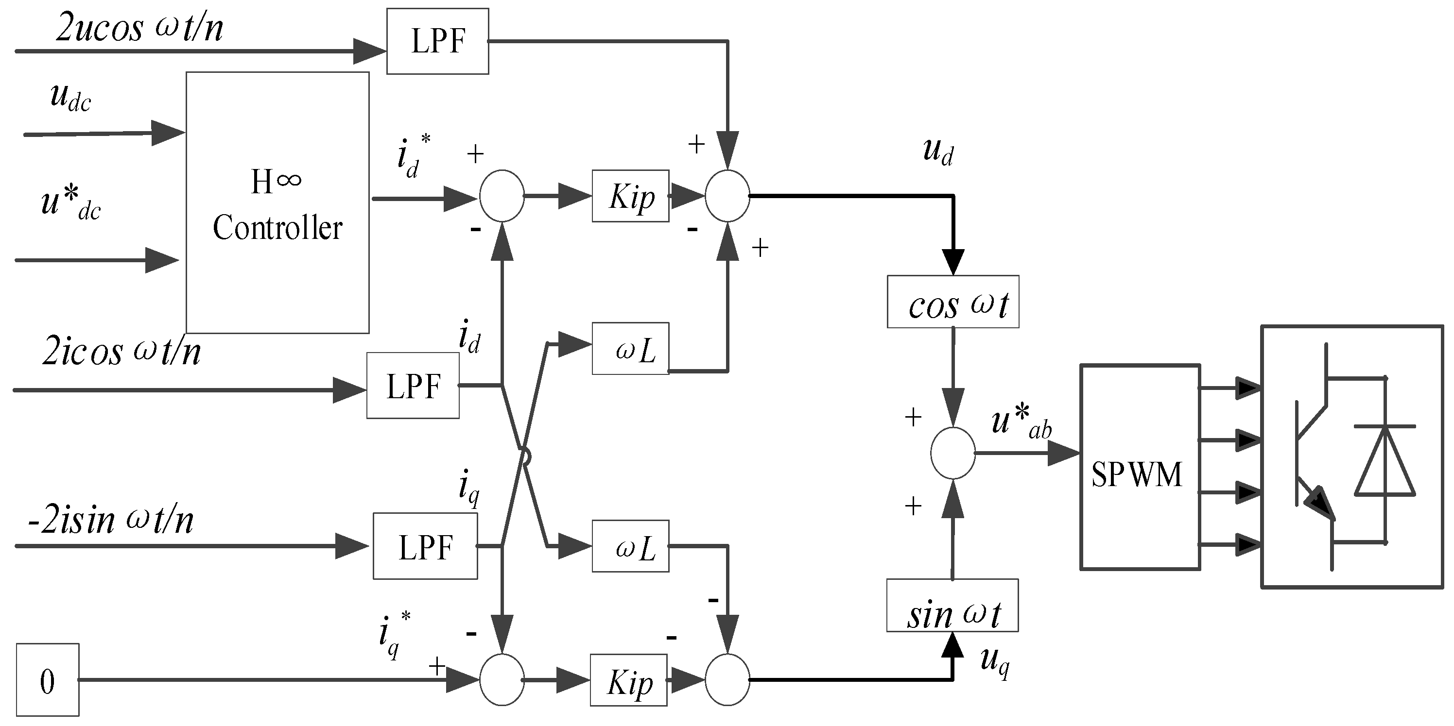
The controller of the line-side converter of EMUs based on H∞ control is shown in Figure 5.

The function of the low-pass filter (LPF) is to block high-frequency signals and preserve the low-frequency signals.

3. Simulation and Analysis for the Dual Line-Side Converter

In a conventional PI system, the expected performance of voltage and current control in different load conditions can be obtained through adjusting the proportion coefficient and integral coefficient generally. According to [16,18,20,21], if the real situations of the EMUs’ converter are considered, the control parameters based on the H∞ controller are set through the PSO in (18). In addition, the parameters of the weight function and the optimal values are listed in

Table 1. Parameters of the weight function and optimal values.

Parameters	Max Value	Min Value	Optimal Value
Ka	100	1 × 10−4	9
Kb	200	10	12
Kc	100	0.001	10
Kd	200	1 × 10−5	45
Ke	100	1 × 10−4	69
Kf	200	0.01	6
Kg	10	1.0	1
$\gamma$	1	0	1

.

$$K={\left[\begin{array}{ccc}0.2& 0.6& 0.4\end{array}\right]}^T$$

(18)

3.1. Off-Line Simulation

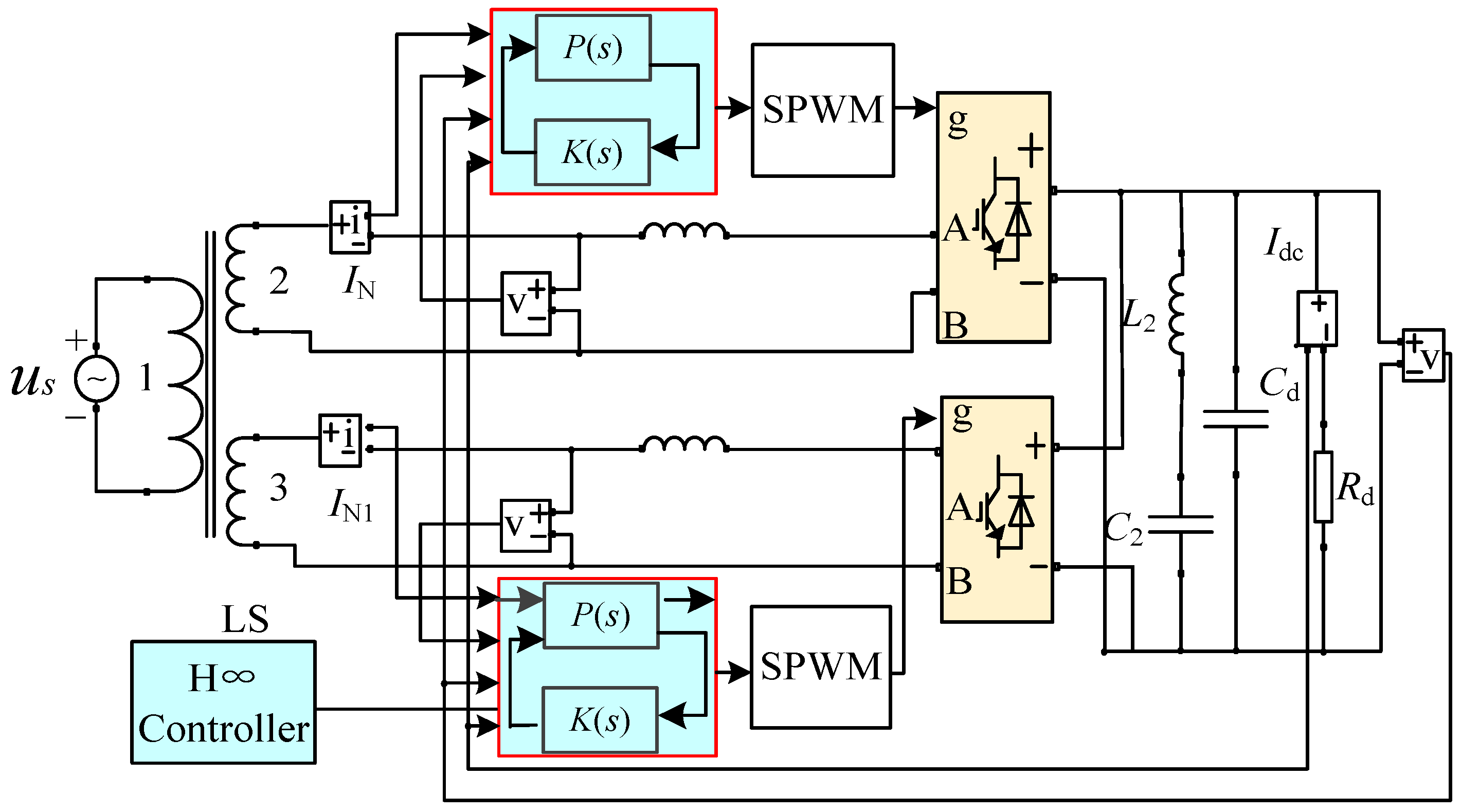
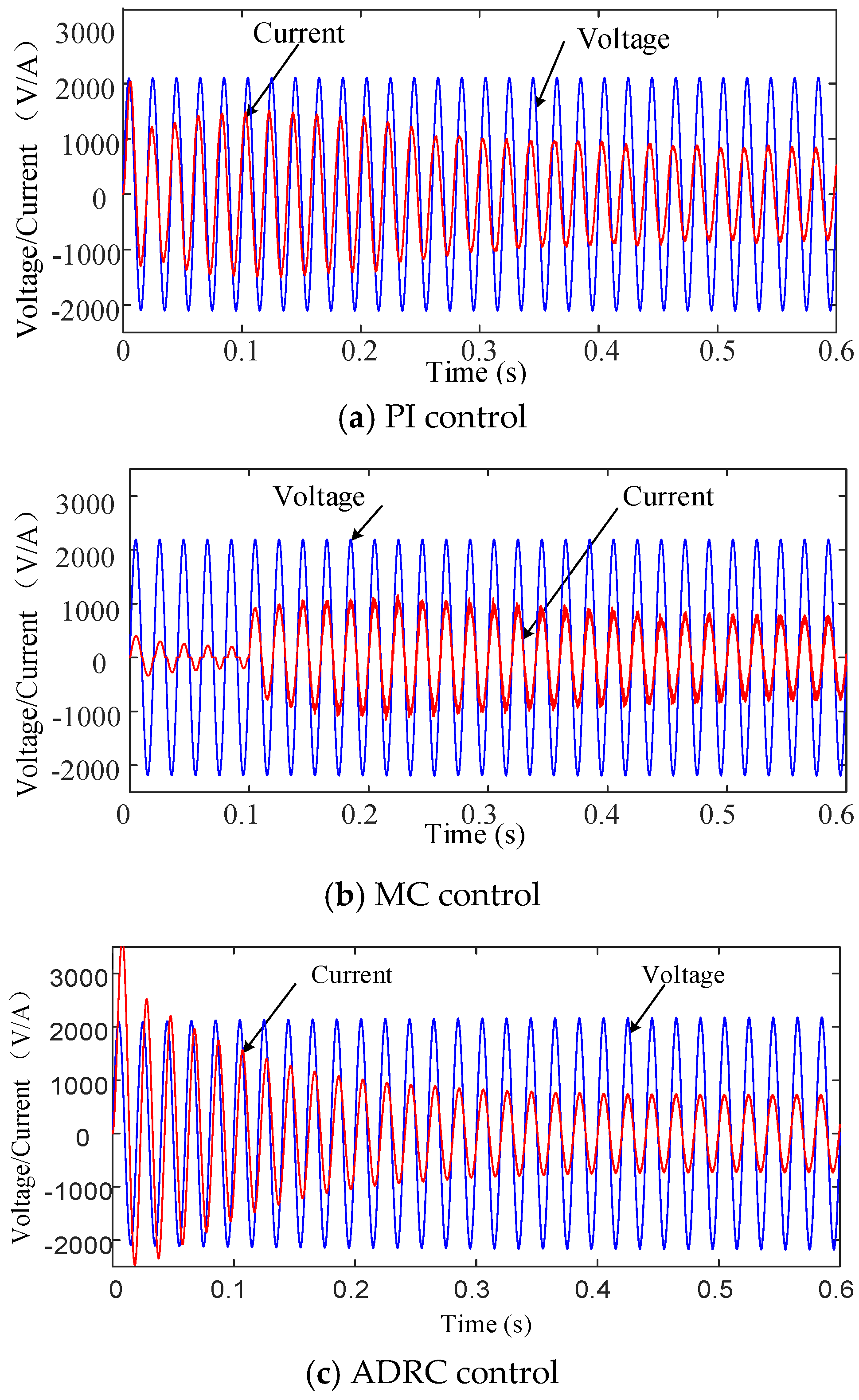
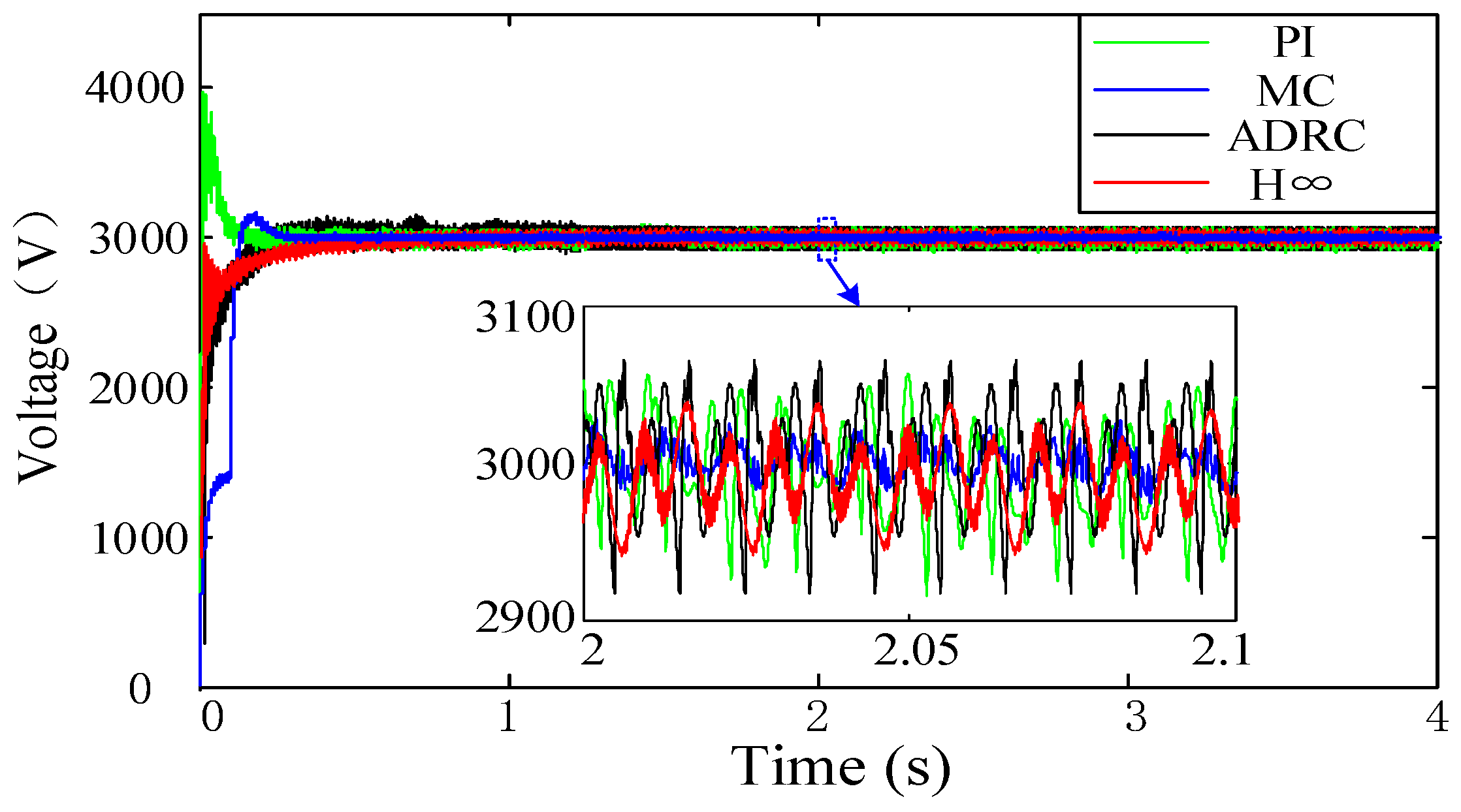
An off-line simulation model of a twofold four quadrant line-side converter of EMUs is built as shown in Figure 6. The parameters are listed in

Table A2. Component parameters of the EMUs’ converter.

System Component	Value
Input voltage	us = 1550 V
AC-side inductance	L = 4.7 mH
Load resistance	Rd = 10 Ω
DC-link reference voltage	udc = 3000 V
Switching frequency	fs = 350 Hz
Sampling frequency	fc = 10.0 kHz
DC-link Capacitance	Cd = 3 mF

, and a bipolar carrier sinusoidal pulse width modulation SPWM algorithm is adopted in the SPWM. The adjustable parameters of the PI controller have been tuned to the appropriate values. Based on the PI controller, MC controller, ADRC controller, and H∞ controller, the waveforms of voltage and current of the line-side converter in a steady state are shown in Figure 7 and Figure 8, respectively. The performance indexes at the DC-link voltage of the line-side converter are listed in

Table 2. Performance indexes of DC voltage for the converter.

Performance	PI Control	MC	ADRC	H∞
Overshoot (%)	16.7	5.5	0.8	0.3
Peak time (s)	0.0125	0.182	None	None
Adjustment time (s)	0.15	0.33	0.18	0.2
Voltage fluctuation (V)	±70	±30	±70	±55

.

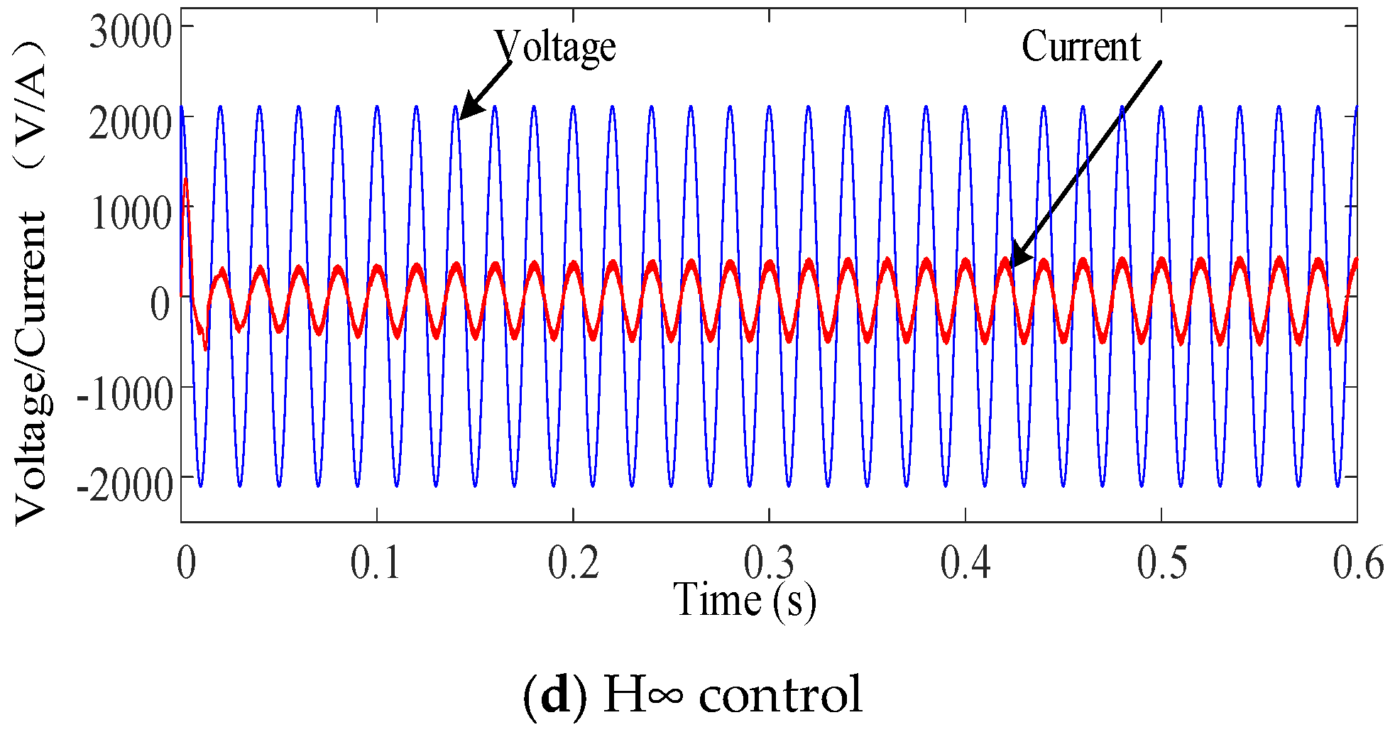
Under a stable state, the line-side converter of EMUs operates in the converter mode, and the energy flows from the traction network to EMUs. In Figure 7a, the line current increases up to 0.1 s and then gradually stabilizes. In Figure 7b, the line current is small at starting and suddenly increases at 0.1s, then the line current tends to stabilize after 0.35s. In Figure 7c,d, the line current is large at the beginning. The line current in Figure 7c decreases gradually, but the line current in Figure 7d increases gradually. And the stable duration of the line current in Figure 7c and Figure 7d is 0.18s and 0.2s, respectively.

From Figure 8 and Table 2, it can be seen that the four controllers all have good performances.

The voltage fluctuation of the H∞ controller is better than the PI and ADRC controllers, which is only ±55V. The voltage overshoot of the PI controller is 16.7%, while the overshoot of the H∞ controller is only 0.3%. Compared with the MC controller, the adjustment time of the H∞ controller is reduced by 39.4%. From Figure 8 and Table 2, it is shown that the peak time of the H∞ controller is much smaller than the peak time of the MC controller.

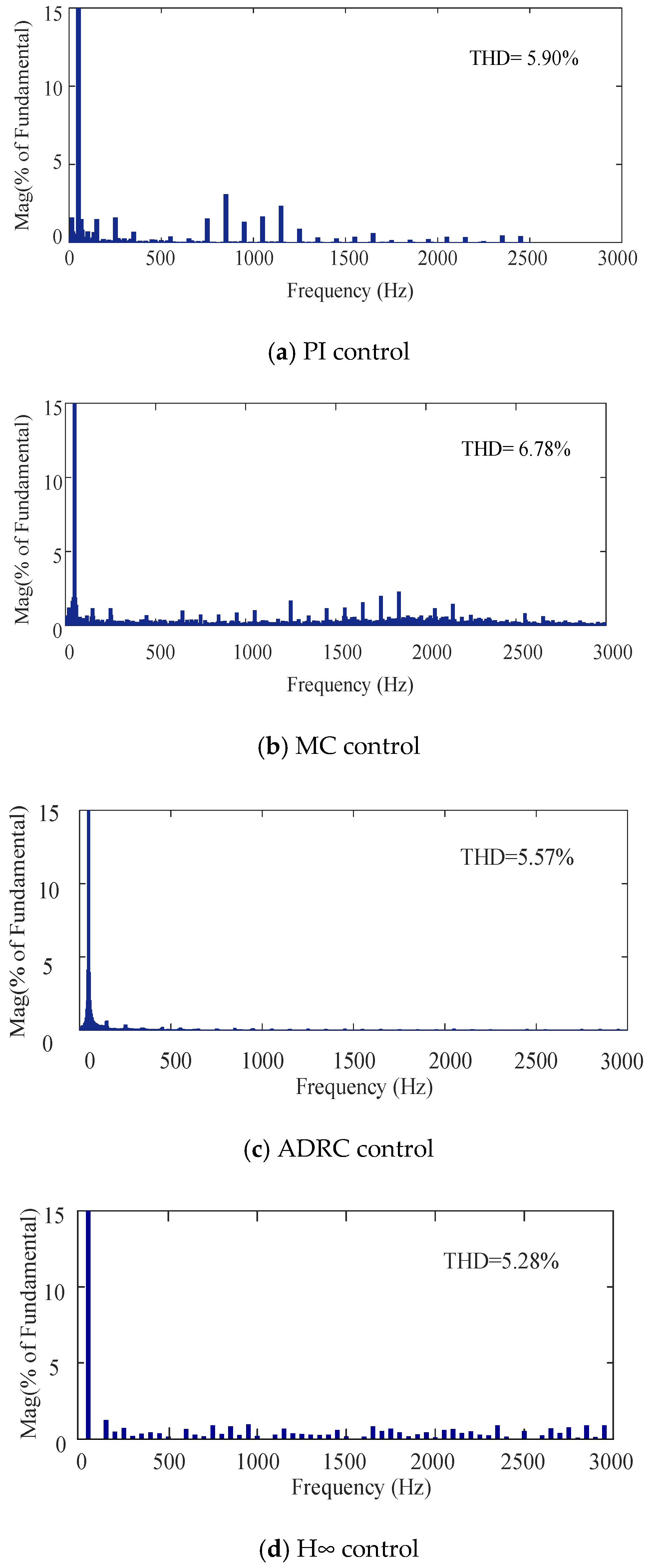
Through the fast Fourier transform (FFT) method, Figure 9a–c show that the line current total harmonic distortion (THD) of line-side converter of EMUs based on the PI controller, MC controller and ADRC controller are 5.90%, 6.78% and 5.57% respectively. The line current THD of line-side converter of EMUs based on the H∞ controller is the smallest than that of the other three controllers, which is 5.28%. Thus, the H∞ controller has better static performance and dynamic performances.

3.2. Real-Time Simulation

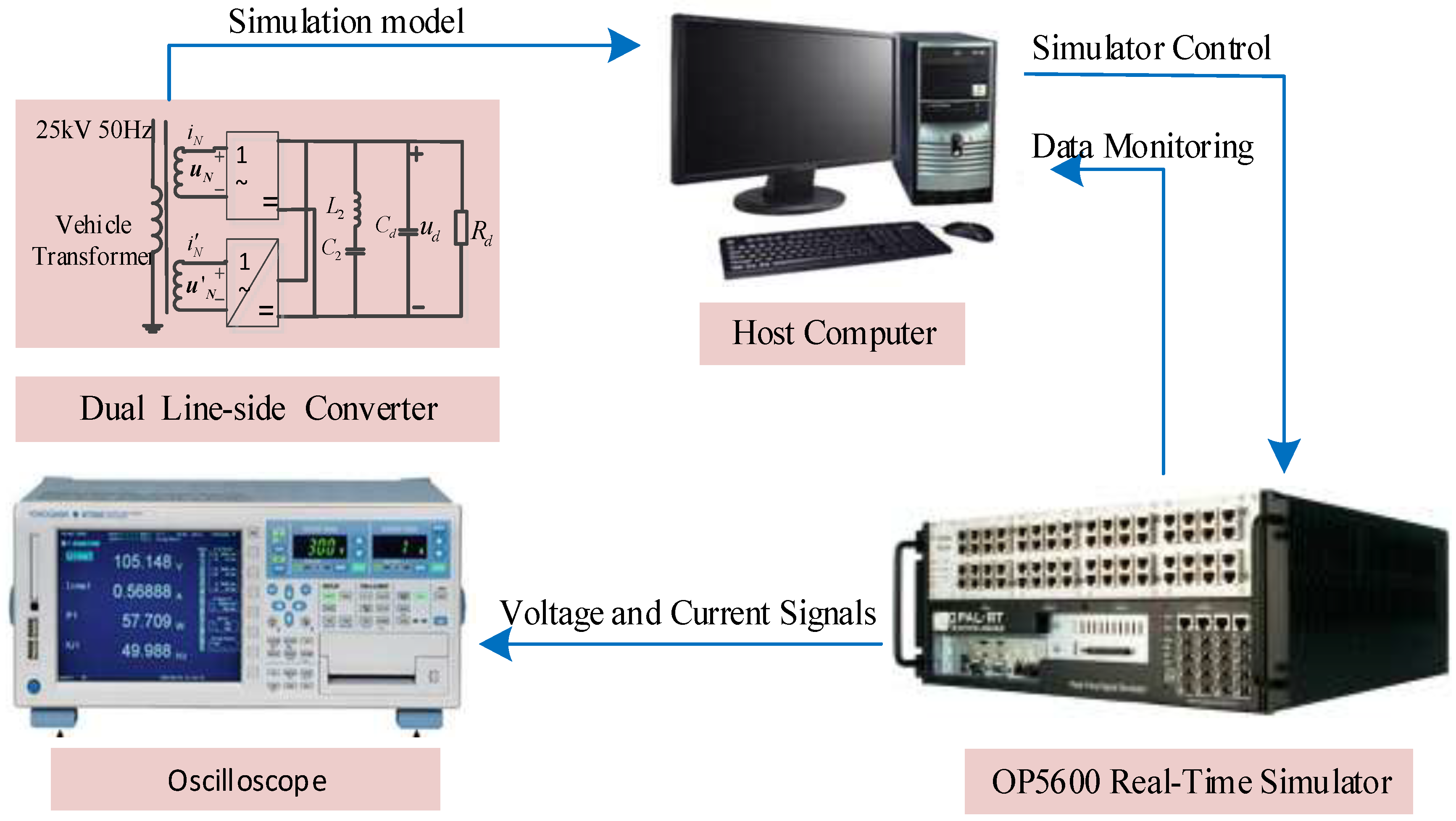
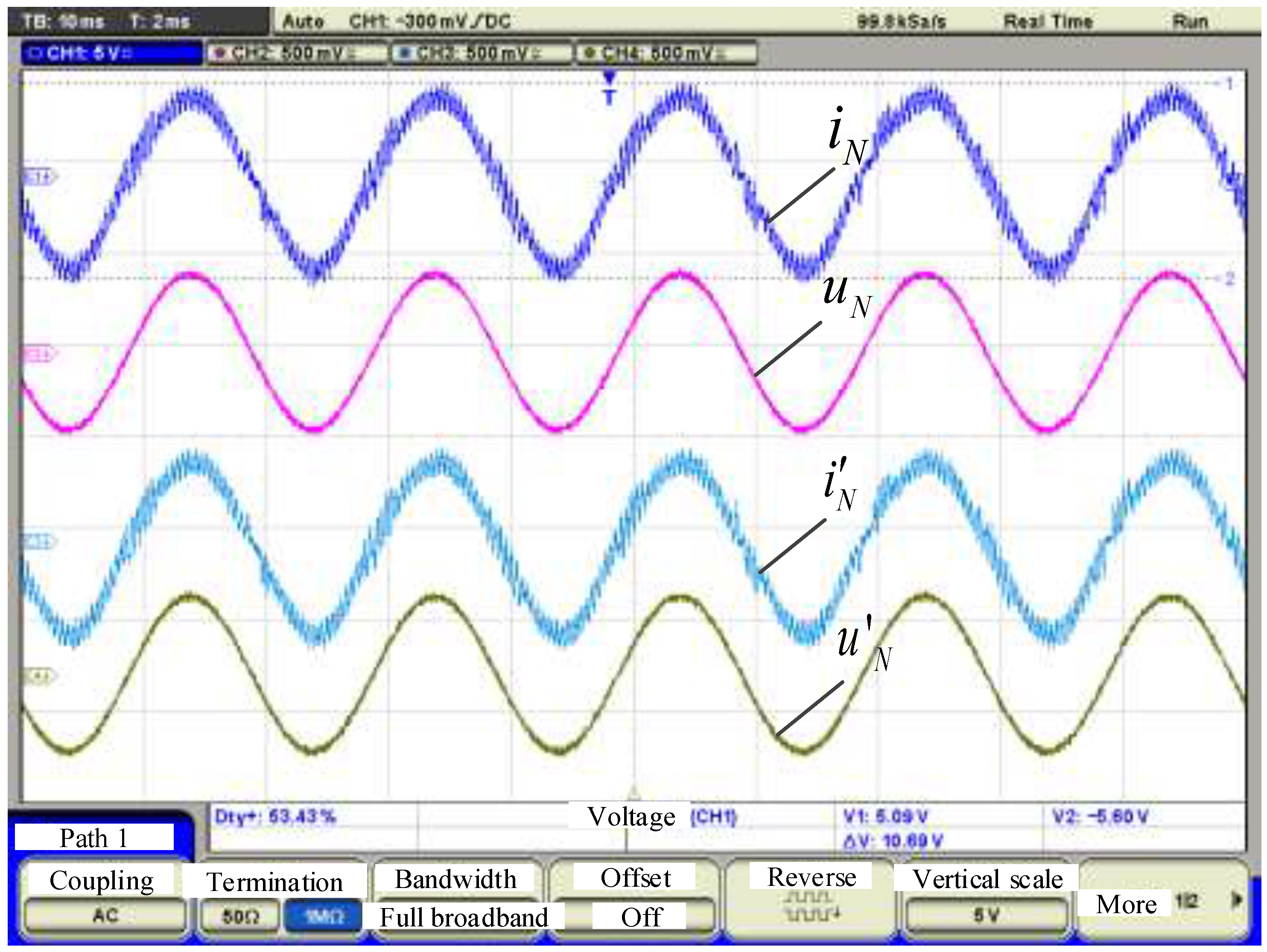
To further validate the performance of the H∞ controller, simulation and experimental tests based on the H∞ controller are carried out. The experimental platform includes an RT-LAB simulator OP5600 (Opal-RT Technologies, Montreal, QC, Canada) and a computer as a real-time control interface as shown in Figure 10. The parameters of real-time simulation are the same as those for the off-line simulation. The waveforms based on the H∞ controller in the steady state are shown in Figure 11. ${\mathit{i}}_{\mathit{N}}$ and ${{\mathit{i}}^{\prime }}_{\mathit{N}}$ in Figure 11 represent the two currents of the dual line-side converter, respectively. ${\mathit{u}}_{\mathit{N}}$ and ${{\mathit{u}}^{\prime }}_{\mathit{N}}$ in Figure 11 represent the two voltages of the dual line-side converter, respectively. The waveforms of the voltage and current are both smooth and sinusoidal generally and in phase without distinct distortion. The results further validate the performance of the H∞ controller.

4. System Verification

4.1. Reduced-Order Model of a Traction Network

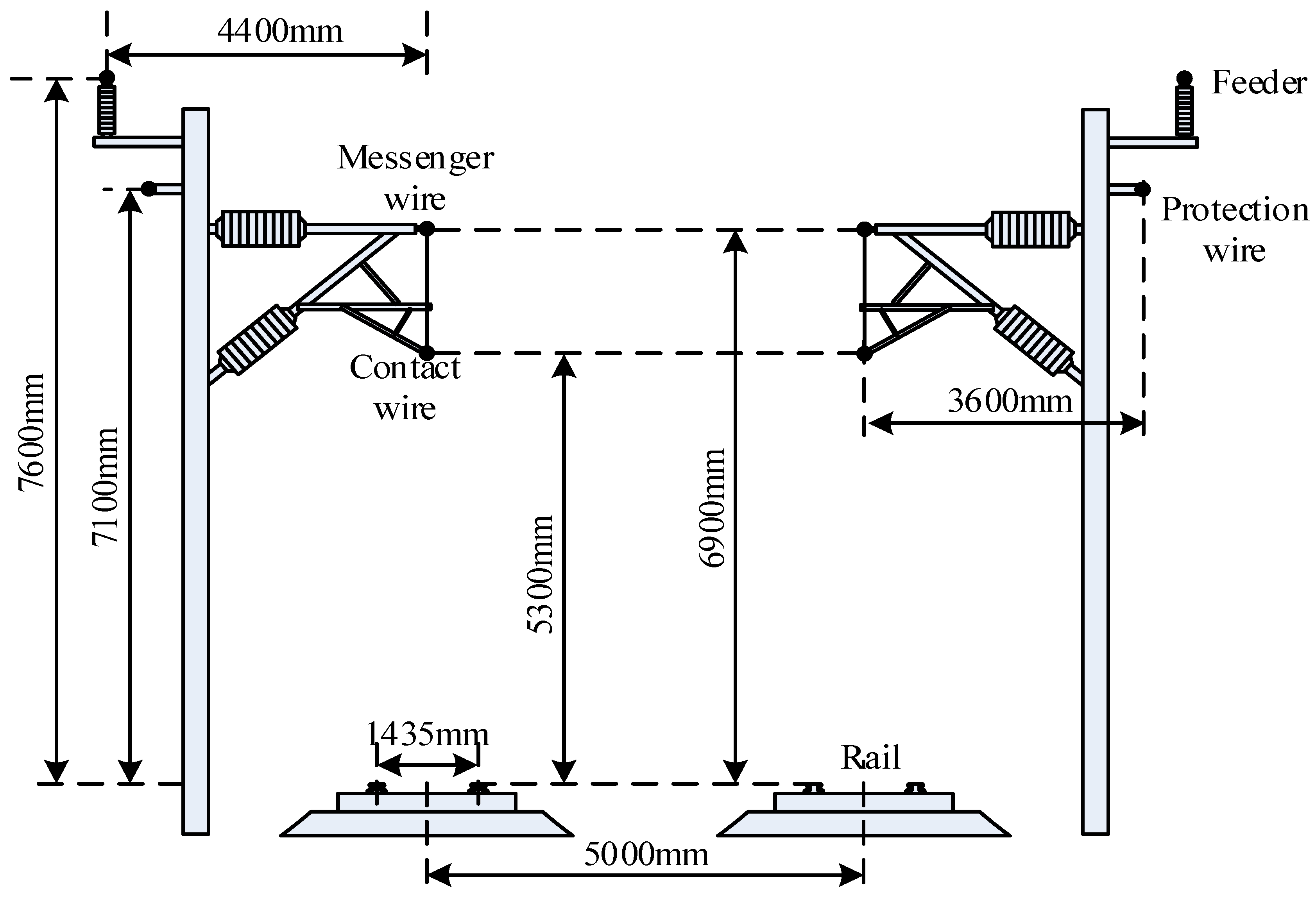
To further verify the LFO suppression effect, a whole traction network model should be built. A traction network is a set of a special kind of multi-conductor single-phase power transmission lines, which consists of a feeder line (F, Z_FF), a messenger wire (M, Z_MM), a contact wire (C, Z_CC), a rail (R, Z_RR), and a protection wire (PW). In order to facilitate the research object, the method of conductor reduced order and merging is adopted to simplify the traction network. Thus, the reduced order model of the traction network can be established with the calculated parameters. The major parameters of the traction network lines are listed in

Table 3. Major parameters of traction network lines.

Conductor	Type DC	Resistance (Ω/km)	Calculation Radius (mm)
C	CuMg-150	0.1191	7.2
R	UIC-60	0.135	12.79
PW	LGJ-120	0.286	4.567
F	2 × LGJ-185	0.082	9.51
M	THJ-120	0.181	7.0

C: contact wire; R: rail; PW: protection wire; F: feeder line; M: messenger wire.

.

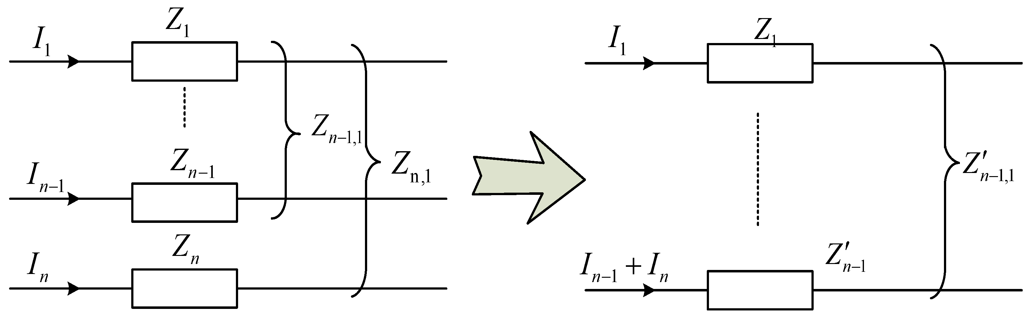
For a single conductor in the traction network, as shown in Figure 12, the self-impedance and the mutual-impedance can be calculated by Carson theory and the self-stiffness and the mutual-stiffness can be obtained in [22]. Thus, the parameters of each conductor can be obtained. Through the merging of conductors circularly, as shown in Figure 13, the wires can be simplified to be one equivalent conductor. The equivalent impedance and admittance of the traction network per unit length can be calculated out as (19) and (20).

$$\{\begin{array}{l}{Z}_{ii}=r_i+0.049+j\omega \frac{{\mu }_0}{2\mathsf{\pi }}\ln \frac{Dg}{R_i}\\ Z_{ij}=Z_{ji}=0.05+j\omega \frac{{\mu }_0}{2\mathsf{\pi }}\lg \frac{Dg}{d_{ij}}\end{array}$$

(19)

$$\{\begin{array}{l}{P}_{ii}=\frac{1}{2\mathsf{\pi }{\epsilon }_0}\ln \frac{2h_i}{R_i}\\ P_{ij}=P_{ji}=\frac{1}{2\mathsf{\pi }{\epsilon }_0}\ln \frac{D_{ij}}{d_{ij}}\end{array}$$

(20)

where $Z_{ii}$ is the self-impedance of conductor i, $r_i$ is the unit length impedance of conductor i, $\omega$ is the angular frequency, ${\mu }_0/2\mathsf{\pi }=2\times {10}^{-4}$ H/km, $D_g$ is the equivalent depth of the conductor–ground loop, $R_i$ is the equivalent radius, $Z_{ij}$ is the mutual-impedance between the conductor i and the conductor j, $d_{ij}$ is the distance between the conductor i and the conductor j, $P_{ii}$ is the self-admittance of wire i, ${\epsilon }_0=1\times {10}^{-6}/(36\mathsf{\pi })$ and it is the vacuum dielectric constant, $h_i$ is the height of the wire i, $P_{ij}$ is the mutual-admittance between the wire i and the wire j, and $D_{ij}$ is the distance between the wire i and the image of the wire j.

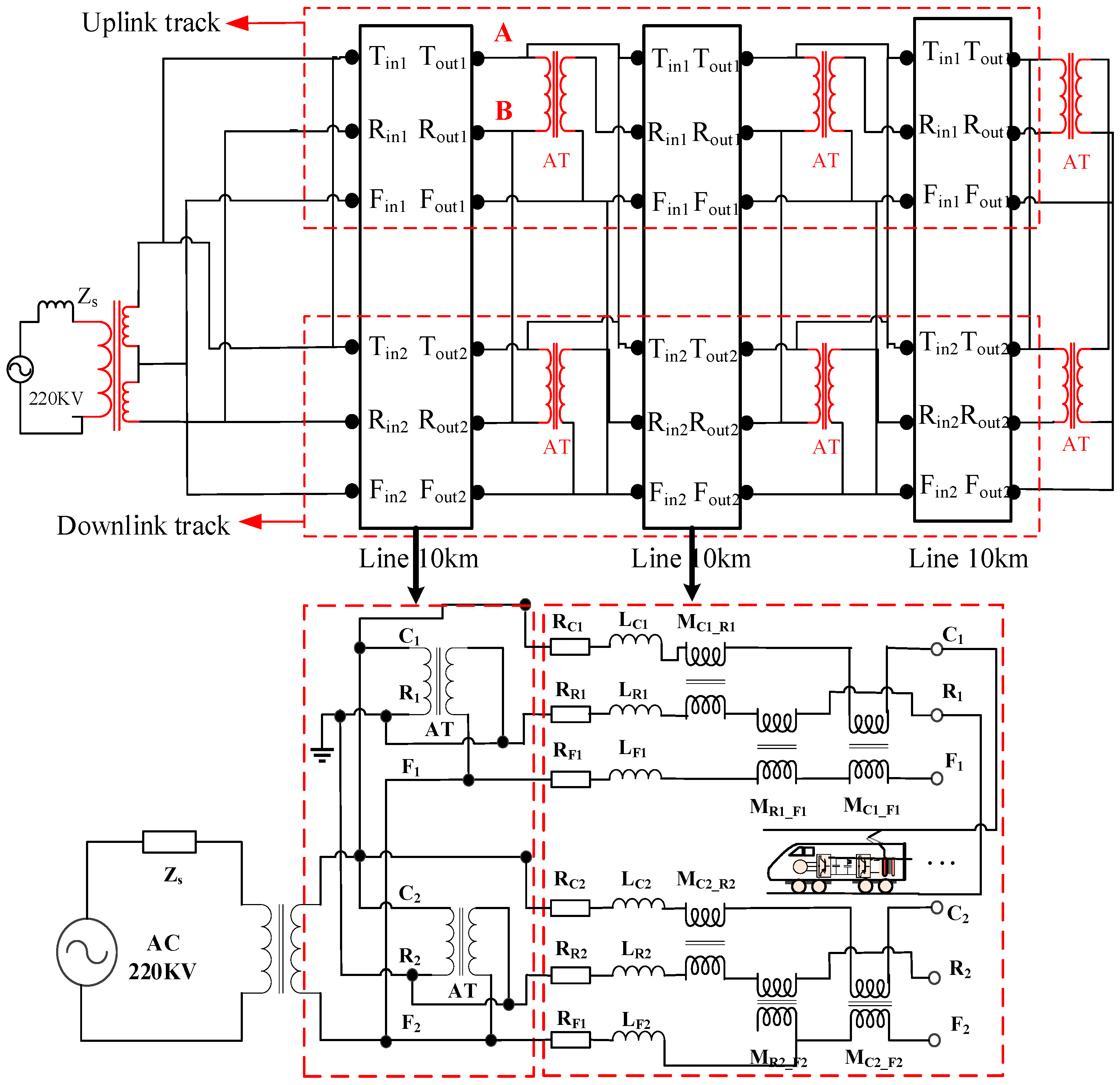
Cascading the model of the traction network per unit length, the simulation model of the whole traction network can be constructed as shown in Figure 14. The corresponding electrical parameters of the test system are listed in

Table A1. Electrical parameters of the test system.

Traction Substation
Power utility short capacity	10 GVA
Rated voltages	220 × (1 ± 2 × 2.5%)/2 × 27.5 kV
Rated power	50/31.5/31.5 MVA
Short-circuit voltage	10.5%
Short-circuit losses	140.7 kW
Auto Transform in Auto Transform Station
Rated voltages	55/27.5 kV
Rated power	35 MVA
Short-circuit voltage	1.6%
Short-circuit losses	57.271 kW
Earth
Earth resistivity	100 Ω/m
Rail to earth conductance	2 S/km
Traction substation and auto transform station earth network to Earth	4 S, 2 S

. And autotransformer (AT) is a special transformer in which the primary winding and the secondary winding are on the same tuning winding.

4.2. Simulation of Multi-EMUs Accessed in the Traction Network Based on PI Control

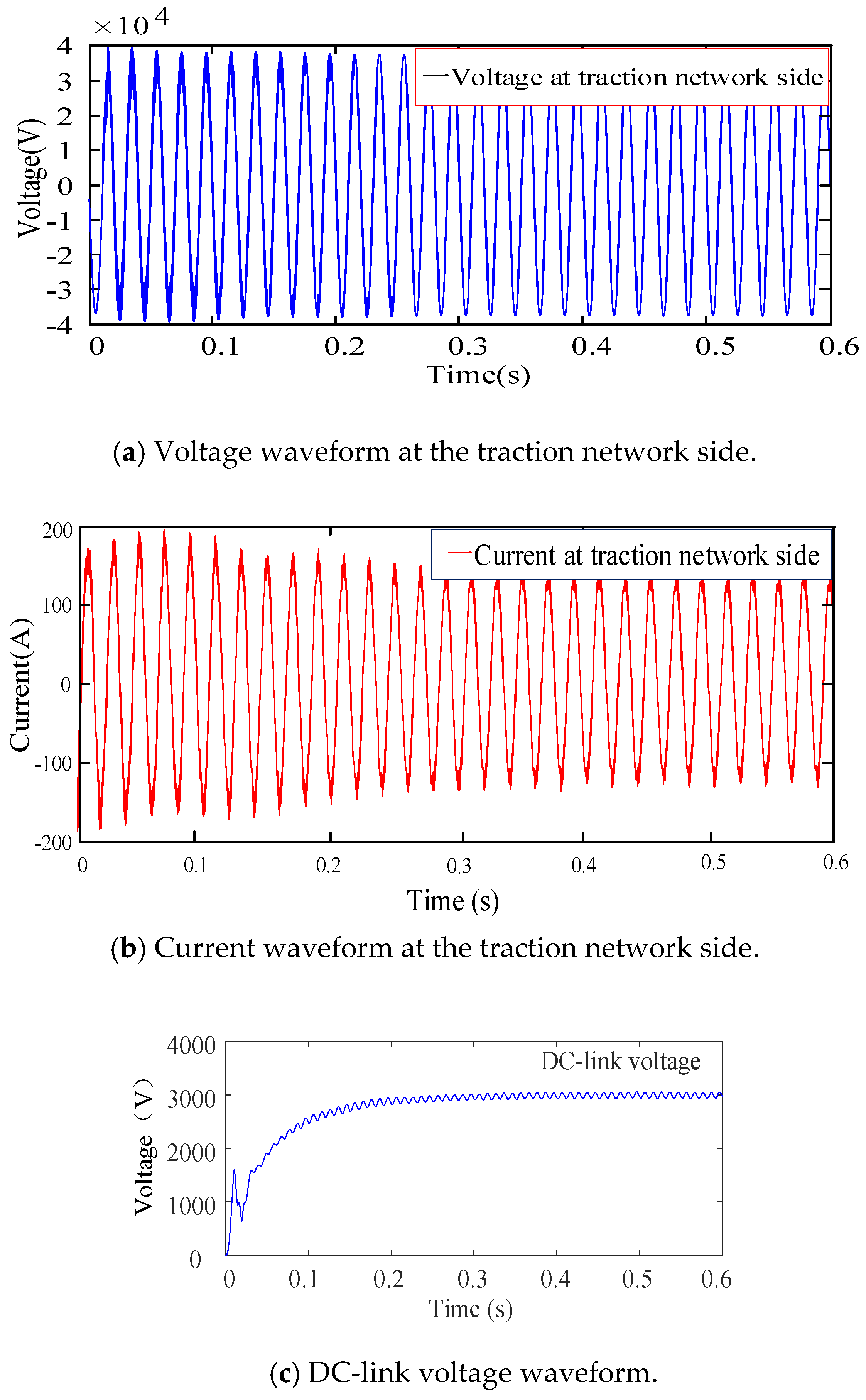
In Figure 14, n EMUs are connected to the position between A and B in the uplink traction substation in traction network. In Figure 15, the fluctuation of voltage and current of the traction network is small when single EMU is connected. The traction network current is enlarged by 100 times to facilitate the observation of the LFO phenomenon. The output DC-link voltage is stable at 3000V and the voltage fluctuation is ±100 V. The THD of the current in traction network side is 25.35%. Therefore, the coupling system of EMUs–traction network is stable. The voltage and current waveforms when 6 EMUs are connected are shown in Figure 16.

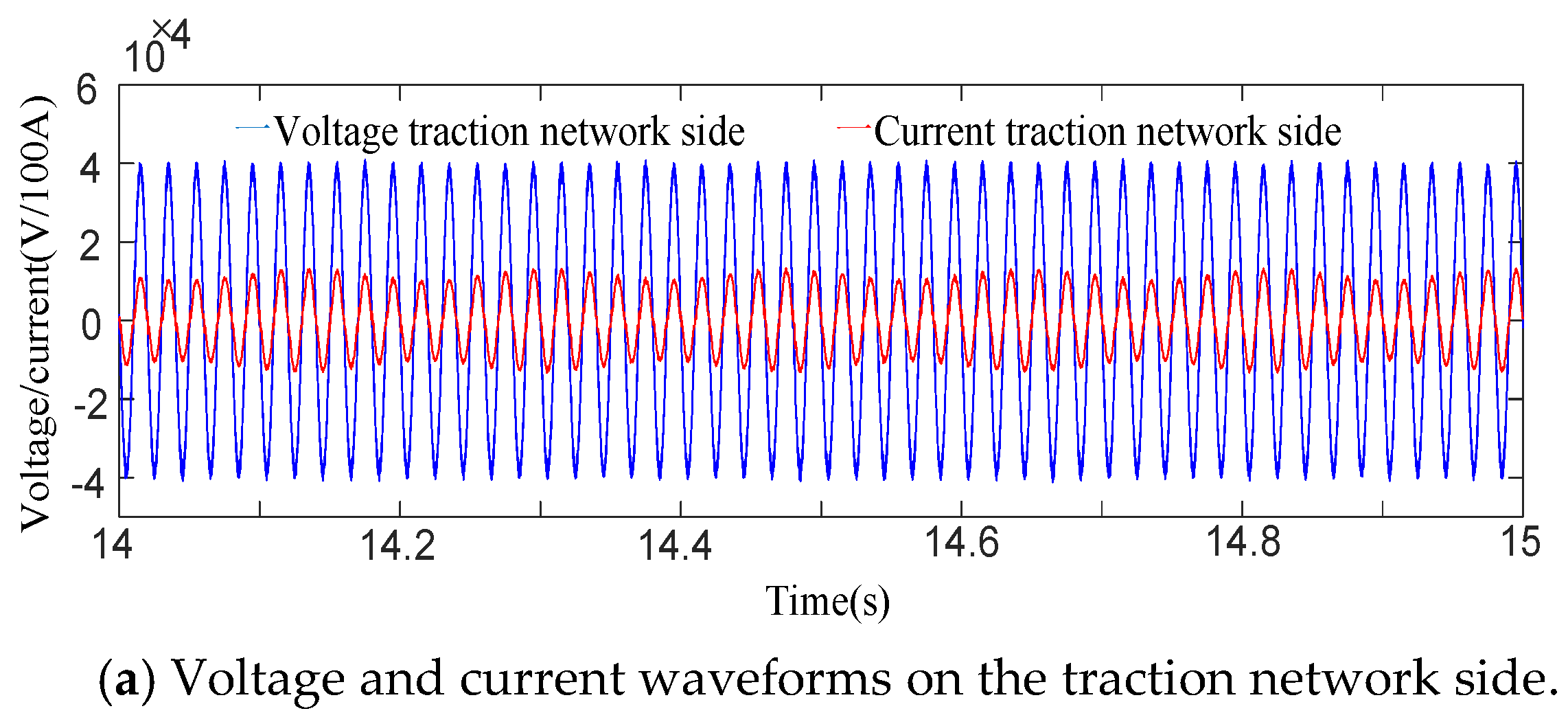
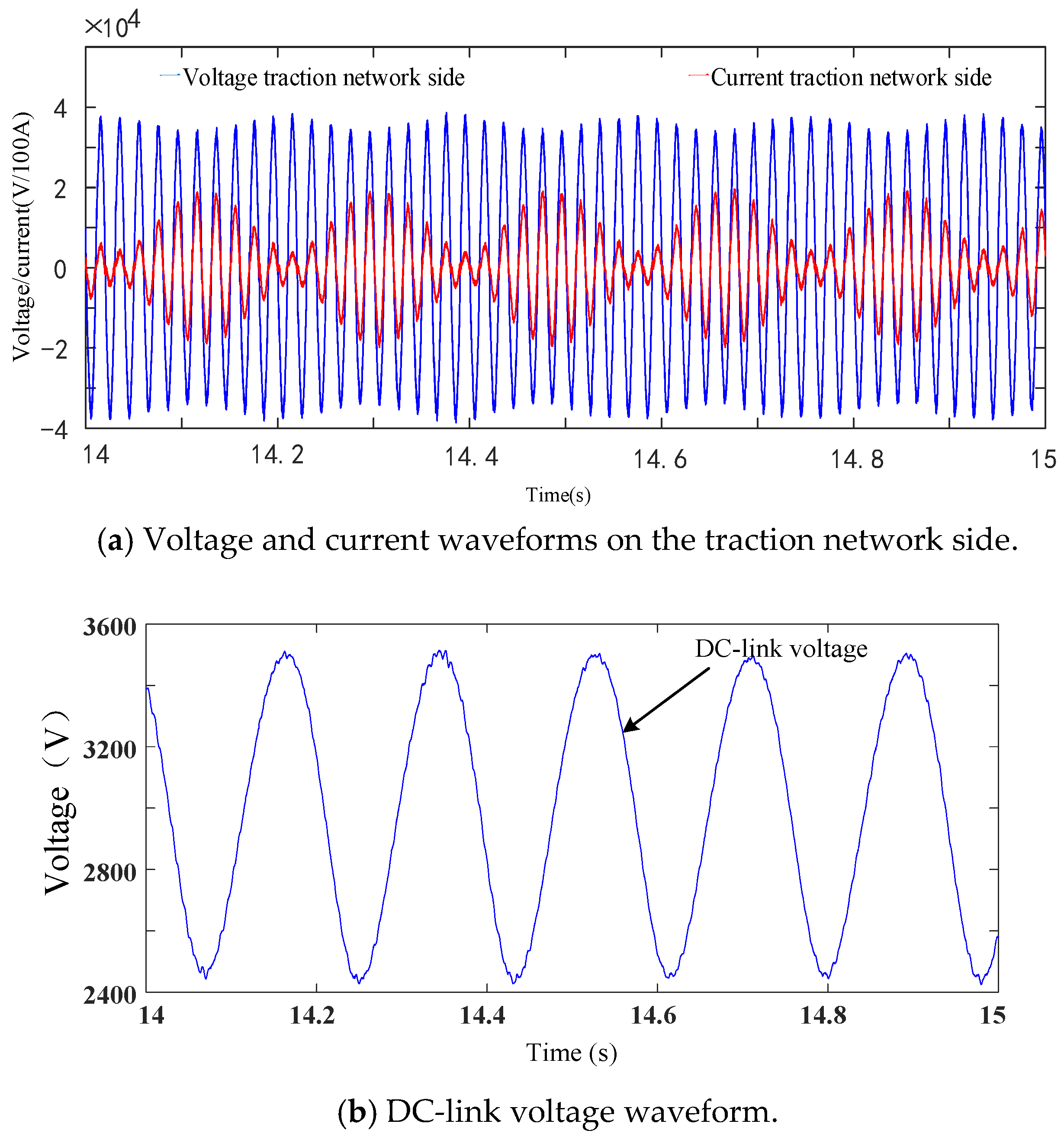
As illustrated in Figure 16, the low-frequency modulation signal appears in the voltage and current of traction network, and the oscillation frequency is about 5.6 Hz. In Figure 16a, the voltage peak of traction network fluctuates between 33 kV and 39 kV. In Figure 16b, the fluctuation of DC-link voltage is ±600V, which fluctuates more severely than that in Figure 15b. It can be found that the instantaneous fluctuation of electric quantities indicates that the increase of load would result in the increase of voltage and current fluctuation, and the dynamic tracking performance of PI controller would decrease. The fluctuation of the line voltage and current of EMUs would result in the poor performance of converter and even the traction blockade.

4.3. Simulation of Multi-EMUs Accessed in Traction Network Based on H∞ Control

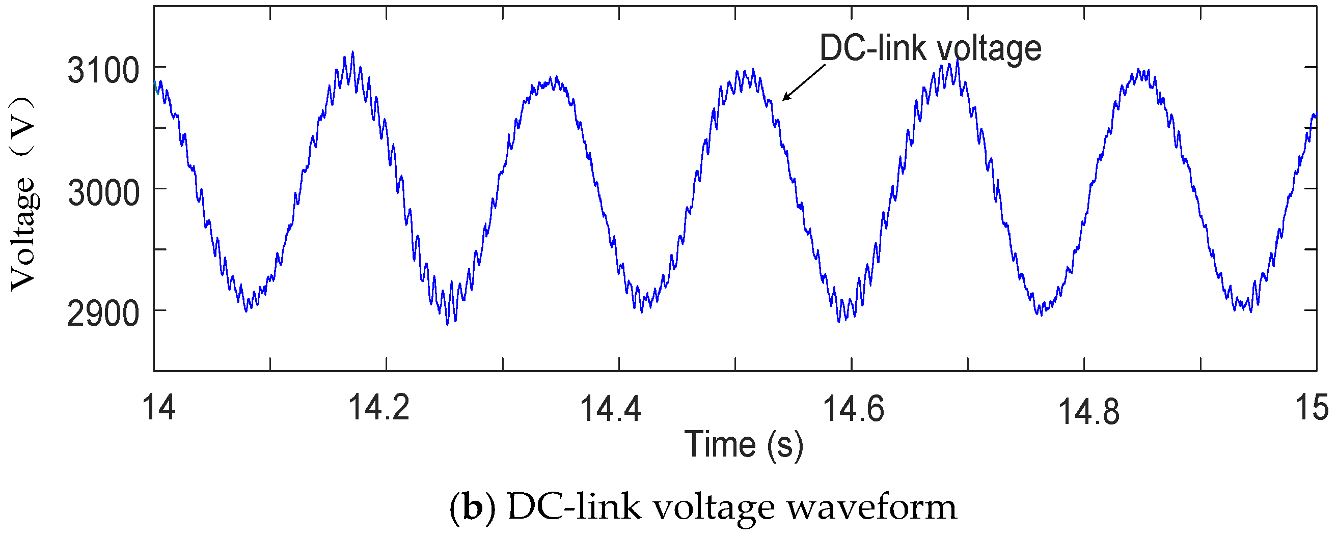
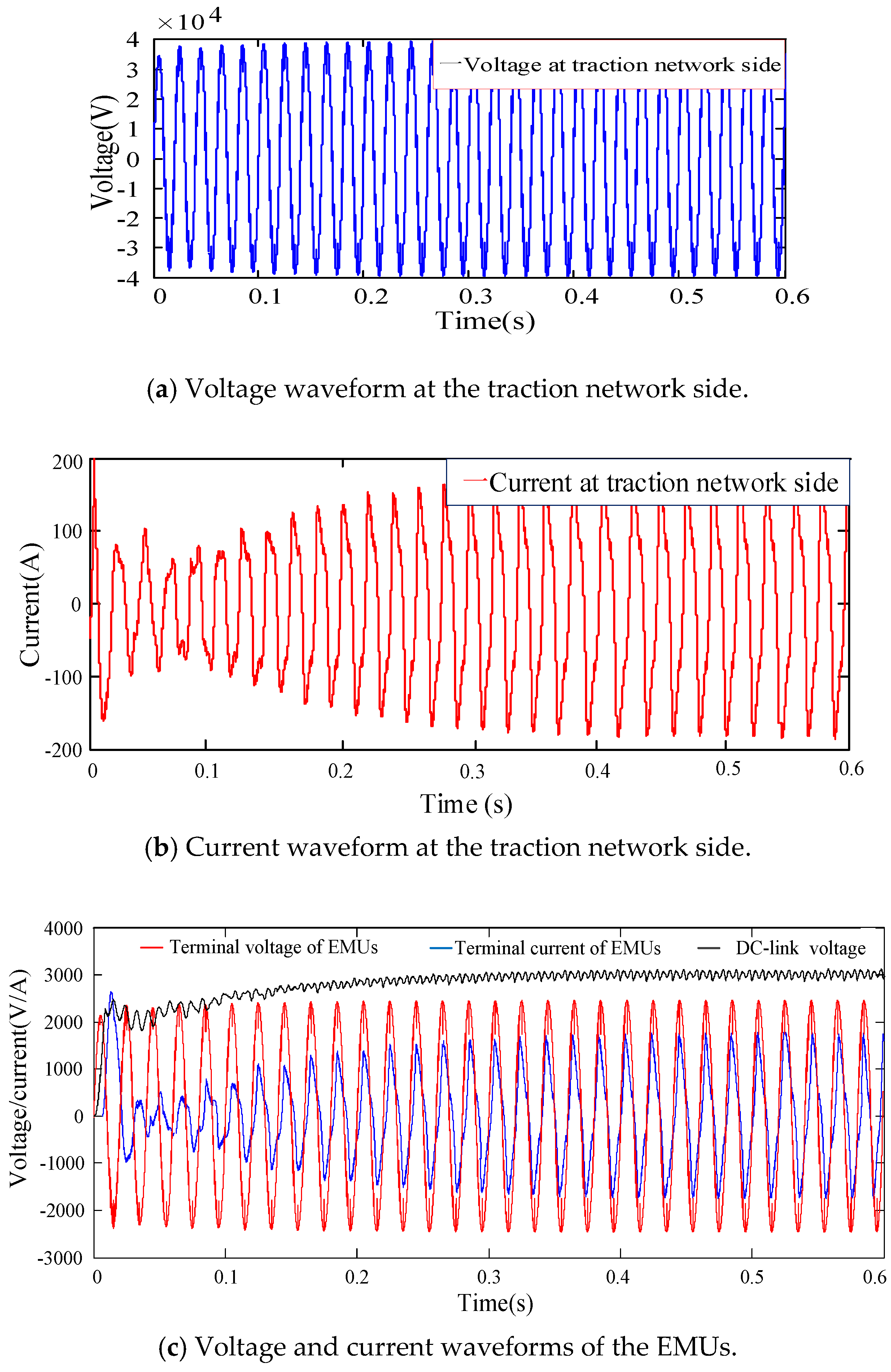
Based on the H∞ controller, when a single EMU is accessed in the traction network, the coupled EMUs–traction network system is stable, and the voltage and current waveforms are shown in Figure 17. The voltage and current of the traction network are stable, and the output DC-link voltage is maintained at 3000 V in Figure 17. When 6 EMUs are accessed in the traction network, the system are still in stable operation. The voltage and current waveforms of the six EMUs are shown in Figure 18. When 6 EMUs are accessed, the fluctuation of voltage and current of the traction network is lower than that in Figure 16a. The current of the traction network is stable at 175 A and the THD of current decreases to 5.64%. The voltage of the traction network fluctuation is within the appropriate range. The DC-link voltage is stable at 3060 V, and the voltage fluctuation is ±50 V. For the static performance, the simulation results show that the electric quantities based on the H∞ controller can stabilize at the reference value, while the static error of the PI controller increases when the load increases.

4.4. Sensitivity of H∞ Control Law Analysis

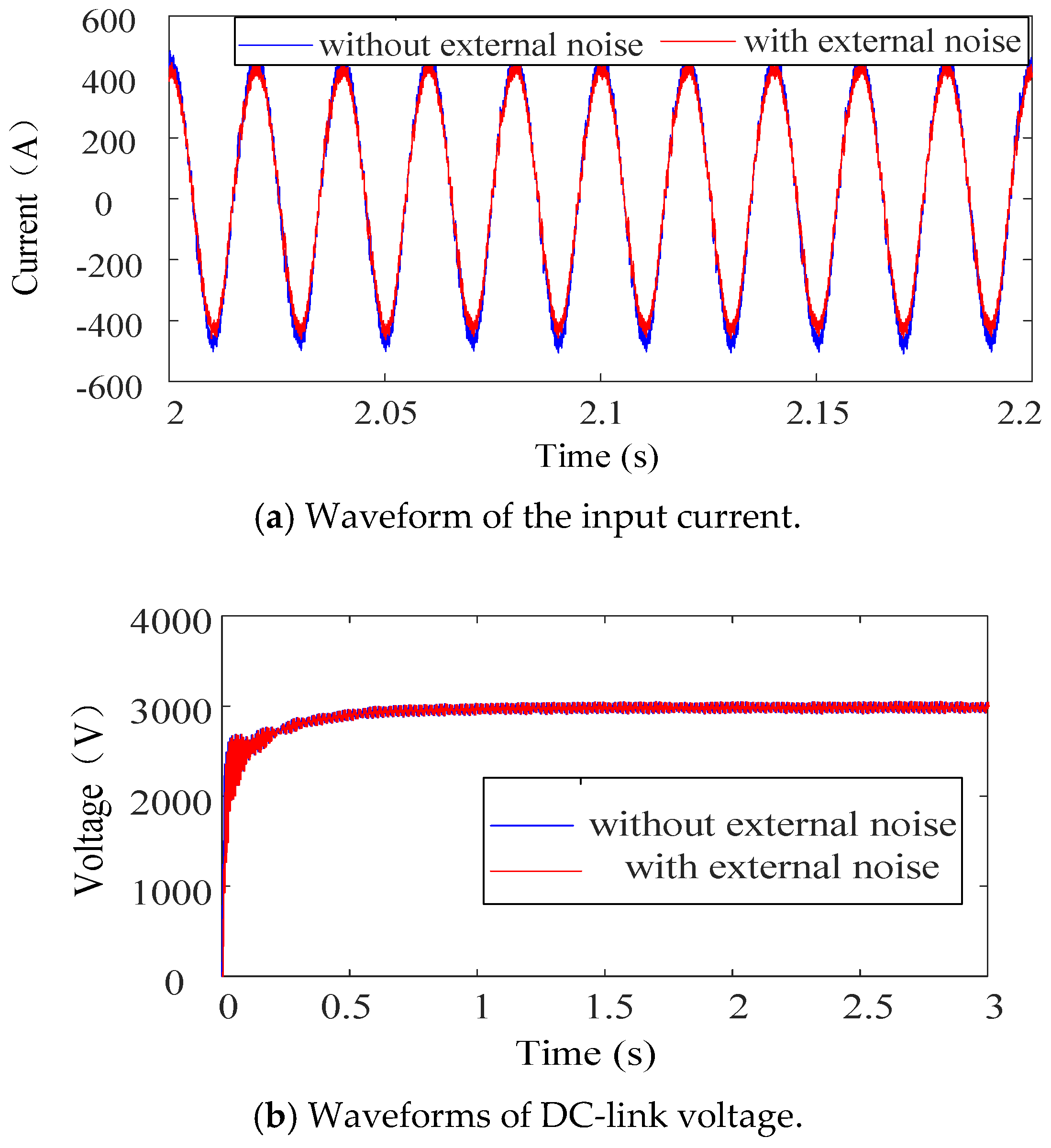
To order to verify the robustness of the H∞ control law, the twofold four-quadrant line-side converter of EMUs is tested by adding some high external noise, and the voltage and current waveforms are shown in Figure 19. In Figure 19a, the waveforms of the line current without and with high external noise are basically consistent, and the THD of the line current without and with high external noise is 5.28% and 5.58%, respectively. In Figure 19b, the waveforms of the DC-link voltage without and with high external noise have almost no difference. Thus, the H∞ control law has good robustness.

To further verify the robustness of the H∞ control law, the model parameters based on the H∞ controller and PI controller are analyzed and compared when seven EMUs are connected in the traction network and the control parameters are kept the same. The model parameters are randomly selected, and they vary from 100 times the original values to 1 percent of the original values. The results are shown in

Table 4. Parameter effect based on PI.

	Parameter	Rs	Ls	Results
Case
1		0.1	0.002	Stable
2		0.5	0.002	Stable
3		1	0.002	Stable
4		10	0.002	Stable, the THD of the current is large
5		0.02	0.002	Stable
6		0.01	0.002	Stable, the THD of the current is large
7		0.001	0.002	Unstable
8		0.1	0.01	Stable
9		0.1	0.02	LFO
10		0.1	0.2	Rectification failure
11		0.1	0.0004	Stable
12		0.1	0.0002	Stable, the THD of the current is large
13		0.1	0.00002	Stable, the THD of the current is large

and

Table 5. Parameter effect based on H∞.

	Parameter	Rs	Ls	Results
Case
1		0.1	0.002	Stable
2		0.5	0.002	Stable
3		1	0.002	Stable
4		10	0.002	Stable, the THD of the current is large
5		0.02	0.002	Stable
6		0.01	0.002	Stable
7		0.001	0.002	Stable
8		0.1	0.01	Stable
9		0.1	0.02	Stable
10		0.1	0.2	Rectification failure
11		0.1	0.0004	Stable
12		0.1	0.0002	Stable
13		0.1	0.00002	Stable

, respectively. In Table 4 and Table 5, it is indicated that the model parameters will affect the control performance and the H∞ control law has better robustness than the PI control law.

To find out the influence factors on the stability of the EMUs–traction network system, the analysis of parameter sensitivity is necessary. The control parameters of the H∞ controller and the PI controller are analyzed and compared when seven EMUs are connected in the traction network. The results are shown in

Table 6. Parameter effect based on PI.

	Parameter	Kp	Ki	Ku	Results
Case
1		0.3	10	1	Stable
2		30	10	1	LFO
3		10	10	1	LFO
4		3	10	1	LFO
5		0.03	10	1	Stable
6		0.01	10	1	Stable
7		0.003	10	1	Stable
8		0.3	1000	1	Rectification failure
9		0.3	500	1	Rectification failure
10		0.3	100	1	Stable
11		0.3	1	1	Stable
12		0.3	0.5	1	Stable
13		0.3	0.1	1	Stable
14		0.3	10	100	Stable
15		0.3	10	50	Stable
16		0.3	10	10	Stable
17		0.3	10	0.5	LFO
18		0.3	10	0.1	LFO
19		0.3	10	0.01	LFO

and

Table 7. Parameter effect based on H∞.

	Parameter	K1	K2	K3	Results
Case
1		0.2	0.6	0.4	Stable
2		20	0.6	0.4	Stable, DC-link voltage is about 12 kV
3		10	0.6	0.4	Stable, DC-link voltage is about 12 kV
4		2	0.6	0.4	Stable, DC-link voltage is about 12 kV
5		0.02	0.6	0.4	Stable
6		0.004	0.6	0.4	Stable
7		0.002	0.6	0.4	Stable
8		0.2	60	0.4	Stable
9		0.2	30	0.4	Stable
10		0.2	6	0.4	Stable
11		0.2	0.06	0.4	Stable
12		0.2	0.012	0.4	Stable
13		0.2	0.006	0.4	Stable
14		0.2	0.6	40	Stable, DC-link voltage is about 12 kV
15		0.2	0.6	20	Stable
16		0.2	0.6	4	Stable
17		0.2	0.6	0.04	Stable
18		0.2	0.6	0.008	Stable
19		0.2	0.6	0.004	Stable

, respectively.

The control parameters vary from 100 times the original values to 1 percent of the original values. In Table 6, it is shown that three control parameters, K_p, K_i and K_u, of the PI controller have an impact on the EMUs–traction network system, and the effect of parameter K_i is less than that of parameters K_p and K_u. The changes of parameters K_p and K_u will result in an LFO. A change in parameter K_i will cause a rectification failure. In Table 7, the control parameter K₁ of the H∞ controller has an impact on the EMUs–traction network system, and parameters K₂ and K₃ have little effect on the system. Changes in parameters K₁ and K₃ can lead to a DC-link voltage of 12 kV. Therefore, the robustness of the H∞ controller for the EMUs–traction network system is verified.

4.5. Discussion

The proposed controller that includes outside disturbances is designed based on the mathematical model for the line-side converter. It can be extended to general situations involving large disturbances and multiple uncertain parameters. The experiments based on off-line and real-time simulations are implemented and tested, and the control parameters based on the H∞ controller and the PI controller are analyzed in this paper. Through the analysis of theory and the verification of simulation, it is proved that the H∞ controller has better performance than the PI controller.

(1)

Better dynamic performance, such as smaller overshoot, shorter peak time and smaller voltage fluctuation.

(2)

Better static performance with rated load.

(3)

The significant suppression capability of LFO in EMUs–traction network system.

Besides, it can be found that the model and control parameters based on the PI controller have a greater impact on the stability of the EMUs–traction network system than those of the H∞ controller. According to Table 4, Table 5, Table 6 and Table 7, some discussions are given as follows.

(1)

In Table 4 and Table 5, the first set of data contains the original values of the model parameters. In Table 4, when the model parameter Rs decreases or Ls increases, the EMUs–traction network system becomes more unstable. LFO or a rectification failure will occur in the system based on PI control when the model parameters change, and the THD of the current will be large. In Table 5, the system is less affected when the model parameters change. Only when the model parameter Ls is expanded to 100 times will a rectification failure occur in the system based on H∞ control. Thus, H∞ control has better robustness than PI control.

(2)

In Table 6, the first set of data is the original value of the PI controller. When the original value of the control parameter K_p is exceeded, LFO will occur. If the control parameter K_u is reduced, LFO will also occur. In addition, it is noted that the set of parameters that exceed the original value of the control parameter K_i will cause a rectification failure. In Table 7, the first set of data contains the original values of the H∞ controller. It can be indicated that the system is stable in all cases. The control parameter K₂ has a little influence on the stability of the system. However, the phenomenon that the DC-link voltage is about 12 kV will appear when the original value of the control parameter K₁ is exceeded. The set of parameters that exceed the original value of the control parameter K₃ can also cause this phenomenon. Actually, 12 kV DC-link voltage is not permitted in real-life operation. Thus, the problem should be studied in the future.

However, as a design method for an optimized system, the optimal control problem of H∞ control theory is difficult to solve. In this paper, H∞ sub-optional control is only used to obtain the approximate solution at present. Although the H∞ control theory can solve robustness problems in the system, some dynamic characteristics of the system are lost. Combined with linear-quadratic-Gaussian control, the H∞ control theory may be a good solution. In addition, since the appropriate weighting functions are difficult to find and the optimal controller is difficult to design, these should be investigated further.

5. Conclusions

The critical factor causing the LFO of EMUs–traction network in high-speed railway is the application of traditional PI controller. In this paper, a nonlinear H∞ controller is designed based on dq frame to improve the load characteristics of line-side converter of the EMUs. The state equation is established and the weighting functions are chosen. And the H∞ controller is designed by solving the Riccati inequalities. The H∞ controller for the line-side converter is analyzed, modeled, and constructed. The simulation and experiment results show that the H∞ controller for the line-side converter has a good performance. The analysis of the sensitivity of H∞ control law shows that the controller has better robustness than PI controller. Besides this, it can ensure the smooth operation of EMUs and efficiently suppress the LFO, which prove the feasibility and the validity of the proposed controller.

References

- Wang, H.; Wu, M. Test and analysis on low frequency oscillation of traction power system voltage caused by EMUs. In Proceedings of the 27th China College Power System and Automation Annual Conference, Qinghuangdao, China, 14–18 October 2011. [Google Scholar]
- Liao, Y.C.; Liu, Z.G.; Zhang, G.N.; Xiang, C. Vehicle-grid system modeling and stability analysis with forbidden region based criterion. IEEE Trans. Power Electron. 2017, 5, 3499–3512. [Google Scholar] [CrossRef]
- Menth, S.; Meyer, M. Low frequency power oscillations in electric railway systems. Eb Elektrische Bahnen 2006, 5, 216–221. [Google Scholar]
- Heising, C.; Bartelt, R.; Oettmeier, M.; Staudt, V. Improvement of low-frequency system stability in 50-Hz railway-power grids by multivariable line-converter control in a distance-variation scenario. In Proceedings of the Electrical Systems for Aircraft, Railway and Ship Propulsion, Bologna, Italy, 19–21 October 2010. [Google Scholar]
- Zhang, G.; Liu, Z.; Yao, S. Suppression of low-frequency oscillation in traction network of high-speed railway based on auto-disturbance rejection control. Trans. Transport. Electrific. 2016, 2, 244–255. [Google Scholar] [CrossRef]
- Wang, H.; Wu, M.; Sun, J. Analysis of low-frequency oscillation in electric railways based on small-signal modeling of vehicle-grid system in dq frame. IEEE Trans. Power Electron. 2015, 9, 5318–5330. [Google Scholar] [CrossRef]
- Assefa, H.Y.; Danielsen, S.; Molinas, M. Impact of PWM switching on modeling of low frequency power oscillation in electrical rail vehicle. In Proceedings of the 13th European Conference on Power Electronics and Applications, Barcelona, Spain, 8–10 September 2009. [Google Scholar]
- Suarez, J.; Ladoux, P.; Roux, N.; Caron, H.; Guillame, E. Measurement of locomotive input admittance to analyse low frequency instability on AC rail networks. In Proceedings of the 2014 International Symposium Power Electronics, Electrical Drives, Automation and Motion (SPEEDAM), Ischia, Italy, 18–20 June 2014. [Google Scholar]
- Oettmeier, M.; Bartelt, R.; Heising, C.; Staudt, V.; Steimel, A. LQ optimized multivariable control for a single-phase 50-kW, 16.7-Hz railway traction line-side converter. In Proceedings of the 13th European Conference on Power Electronics and Applications, Barcelona, Spain, 8–10 September 2009. [Google Scholar]
- Bartelt, R.; Oettmeier, M.; Heising, C.; Staudt, V. Improvement of low-frequency system stability in 16.7-Hz railway power grids by multivariable line-converter control in a multiple traction vehicle scenario. In Proceedings of the Electrical Systems for Aircraft, Railway and Ship Propulsion, Bologna, Italy, 19–21 October 2010. [Google Scholar]
- Wang, Y.; Wang, J.; Zeng, W. H∞ Robust Control of an LCL-Type Grid-Connected Inverter with Large-Scale Grid Impedance Perturbation. Energies 2018, 11, 57. [Google Scholar] [CrossRef]
- Tan, P.; Morrison, R.E.; Holmes, D.G. Voltage from factor control and reactive power compensation in a 25-kV Electrified railway system using a shunt active filter based on voltage detection. IEEE Trans. Ind. Appl. 2003, 2, 575–581. [Google Scholar]
- Jin, W.; Li, Y.; Sun, G. H∞ Repetitive Control Based on Active Damping with Reduced Computation Delay for LCL-Type Grid-Connected Inverters. Energies 2017, 10, 586. [Google Scholar] [CrossRef]
- Zhao, R.; Lu, S.; Tu, L. Design of decentralized controllers for parallel AC-DC system based on effective relative gain array and mixed H2/H∞ control. Power Syst. Protect. Control 2016, 24, 44–51. [Google Scholar]
- Feng, X. Electric Traction AC Drives and Control System; Higher Education Press: Beijing, China, 2009. [Google Scholar]
- Gou, B.; Ge, X.; Wang, S.; Feng, X. An open-switch fault diagnosis method for single-phase PWM rectifier using a model-based approach in high-speed railway electrical traction drive system. IEEE Trans. Power Electron. 2016, 5, 3816–3826. [Google Scholar] [CrossRef]
- Green, A.W.; Boys, J.T.; Gates, G.F. 3-phase voltage sourced reversible rectifier. IEEE Proc. B Elec. Power Appl. 1988, 6, 362–370. [Google Scholar] [CrossRef]
- Wu, G.R.; Xiao, X. Robust speed controller for a PMSM Drive. In Proceedings of the International Power Electronics and Motion Control Conference, Wuhan, China, 17–20 May 2009. [Google Scholar]
- Li, Q.; Chen, W.; Liu, S.; Liu, X. H∞ suboptimal control for proton exchange membrane fuel cell (PEMFC) hybrid power generation system based on modified particle swarm optimization. Power Syst. Prot. Control 2010, 21, 126–131. [Google Scholar]
- Dabra, V.; Paliwal, K.K.; Sharma, P. Optimization of photovoltaic power system: A comparative study. Prot. Control Mod. Power Syst. 2017, 2, 3. [Google Scholar] [CrossRef]
- Saptarshi, D.; Pan, I. On the mixed H-2/H-infinity loop-shaping tradeoffs in fractional-order control of the AVR system. IEEE Trans. Ind. Inf. 2014, 4, 1982–1991. [Google Scholar]
- Lee, H.; Lee, C.; Jang, G.; Kwon, S.H. Harmonic analysis of the Korean high-speed railway using the eight-port representation model. IEEE Trans. Power Deliv. 2002, 2, 979–986. [Google Scholar] [CrossRef]
Figure 1.
Schematic of traction network and electric multiple units (EMUs). PWM: pulse-width modulation; DC: direct current.
Figure 2.
The idea in this paper. LFO: low-frequency oscillation; PSO: particle swarm optimization; PI: proportional integral; MC: multivariable control; ADRC: auto-disturbance rejection control.
Figure 3.
Equivalent circuit of a twofold four-quadrant pulse converter.
Figure 4.
Structures of the mixed-sensitivity problem and the standard H∞ control.
Figure 5.
Block diagram of the H∞ controller.
Figure 6.
Simulation model of the twofold four-quadrant EMUs converter.
Figure 7.
Waveforms of the line voltage and current of the convertor in steady state use.
Figure 8.
Waveforms of the DC-link voltage of the converter.
Figure 9.
Fast Fourier transform (FFT) results of the input current. THD: total harmonic distortion.
Figure 10.
Structure of the real-time online simulation system experimental test platform.
Figure 11.
Waveforms of the line voltage and current with H∞ in the RT-LAB platform.
Figure 12.
Multi-conductor transmission line system of the traction network.
Figure 13.
Impedance reduced-order principle.
Figure 14.
The simulation model of traction power supply system. AC: alternating current.
Figure 15.
Voltage and current waveforms with a single EMU accessed based on the PI controller.
Figure 16.
Voltage and current waveforms with six EMUs accessed based on the PI controller.
Figure 17.
Voltage and current waveforms with a single EMU accessed based on the H∞ controller.
Figure 18.
Voltage and current waveforms with six EMUs accessed based on the H∞ controller.
Figure 19.
Waveforms of voltage and current of the convertor.