Impact of Component Reliability on Large Scale Photovoltaic Systems’ Performance


1
Vattenfall Innovation GmbH, Chausseestrasse 23, 10115 Berlin, Germany
2
Centre for Renewable Energy Systems Technology, School of Mechanical, Electrical and Manufacturing Engineering, Loughborough University, Loughborough, LE11 3TU, UK
3
juwi Renewable Energies Limited, Energie-Allee 1, 55286 Wörrstadt, Germany
4
Fraunhofer-Centre for Silicon-Photovoltaic CSP, Walter-Hülse-Strasse 1, 06120 Halle, Germany
*
Author to whom correspondence should be addressed.
Energies 2018, 11(6), 1579; https://doi.org/10.3390/en11061579
Submission received: 9 February 2018
/
Revised: 24 May 2018
/
Accepted: 12 June 2018
/
Published: 15 June 2018
(This article belongs to the Special Issue PV System Design and Performance)
Abstract
:In this work, the impact of component reliability on large scale photovoltaic (PV) systems’ performance is demonstrated. The analysis is largely based on an extensive field-derived dataset of failure rates of operation ranging from three to five years, derived from different large-scale PV systems. Major system components, such as transformers, are also included, which are shown to have a significant impact on the overall energy lost due to failures. A Fault Tree Analysis (FTA) is used to estimate the impact on reliability and availability for two inverter configurations. A Failure Mode and Effects Analysis (FMEA) is employed to rank failures in different subsystems with regards to occurrence and severity. Estimation of energy losses (EL) is realised based on actual failure probabilities. It is found that the key contributions to reduced energy yield are the extended repair periods of the transformer and the inverter. The very small number of transformer issues (less than 1%) causes disproportionate EL due to the long lead times for a replacement device. Transformer and inverter issues account for about 2/3 of total EL in large scale PV systems (LSPVSs). An optimised monitoring strategy is proposed in order to reduce repair times for the transformer and its contribution to EL.
1. Introduction
The Photovoltaic (PV) sector has grown significantly in recent years, representing a remarkable proportion of the global energy produced by renewable energy sources. By the end of 2016, PV systems reached more than 303 GW in worldwide installed capacity [1]. As the growth rate of PV systems continues to increase, the main concern for investors, owners and stakeholders is to ensure that a PV system generates energy as predicted. Unexpected failures that result in extended downtime periods are detrimental for the financial outcome of the investment. In order to assess the risks imposed by component failures, reliability assessment is carried out during the due diligence of any PV system planning.
Reliability is crucial for system planning and long-term operation, as it allows to facilitate risk assessment and limit revenue losses. It further enables predicting system behaviour over time and planning maintenance strategies accordingly [2]. However, it is commonly limited by lacking robust data. This paper presents an up-to-date dataset of field reliability and its impact on overall systems’ performance with a focus on large scale PV systems (LSPVSs), namely systems with more than 1 MWP installed capacity.
In LSPVSs, reliability is quite complex to carry out due to the variability associated with the system components, namely the PV modules, inverter(s) and other balance of systems (BOSs) components [3,4]. A major part of the existing literature focuses on the reliability assessment of specific components, such as the inverter [5], IGBT switches [6] and largely on the PV modules’ individual elements (encapsulant, bypass diodes etc.) [7,8,9,10]. Much fewer studies, however, discuss the reliability evaluation for the entire PV system, with the majority using oversimplified assumptions, which may lead to controversial observations between simulated and real results, as discussed in more detail in [11]. A number of studies also focus on smaller PV systems. For example, in [12], a large number of residential PV systems are analysed over a period of seven years where failures are mainly grouped into inverter and module faults. In [13], a simulation tool is applied using failure rates imported in literature for small-scale systems, in order to calculate energy losses (EL) when different maintenance scenarios are considered. However, small-scale PV systems may have entirely different characteristics, such as different inverter instrumentation and the lack of certain components such as transformers, combiner boxes and string fuses (for example, domestic systems with up to two strings). Moreover, quality assurance at various project stages and the lack of due diligence and extensive operation and maintenance (O&M) plans lead to many issues going unnoticed in smaller plants [13].
The analysis of LSPVSs is commonly carried out using a fault tree analysis (FTA), as seen in early [14] and more recent [15,16] reliability work. FTAs are used to interpret a physical layout (such a PV system) into a logical diagram (block diagram) whereby each block represents a system component, described by its failure rate. The failure rates for each component determine the reliability of the overall system, and thus every input is important. Commonly, failure rates are assumed constant. More recent work includes dynamic FTAs where failure rates can be described by (time-dependent) probability functions [17]. This is, however, a stochastic approach that does not necessarily rely on actual field values. In fact, most cited works lack realistic, field derived data for their analysis. Freely available datasets such as [18] are outdated and thus are expected to produce unrealistic results for current technologies as also seen in [16]. In some cases, reliability assessment is carried out by using simulated failure models [19] rather than real data. In [20], the impact on EL due to failures has been researched where real data are gathered from different plants but for an operation of only 15 months. In [21], probability distributions were fitted to actual data from a 5-year operation period of a large scale system to predict failure rates and availability. However, this data is not provided. In addition to data availability and accuracy, the inclusion of all possible system components into the reliability model is also a missing factor. For example, in [22], a large system reliability analysis is carried out; however, the element of the transformer is not included.
In this work, a reliability model is presented using a combination of literature-based failure rates and a large collection of field-derived data. This data is provided by the juwi renewable energy systems for system sizes ranging between 1.4 MWP and 3.5 MWP [23]. The field-derived failure rates correspond to system operation of two to seven years (see Table 1). In this study, the failure rates of all electrical components of a large grid-connected PV system are investigated. Two different inverter topologies are considered: string inverters (SI) and central inverters (CIs). Energy and time availability are calculated (as suggested in [24]) and EL due to failures are estimated, using average detection and repair times. The impact of individual components on overall system reliability is discussed through failure mode and effect analysis for each subsystem. Finally, maintenance strategies are proposed for improving energy availability (EA) and cost-effectiveness of large PV systems.
2. Reliability and Availability Modelling
This section summarises the different concepts used for the assessment of performance risks of LSPVS. The aim is to summarise the state of the art and approaches being used in this work.
2.1. Risk Assessment
Risk assessment will be deployed to identify, understand and evaluate the effect of known uncertainties on the objectives of an assessment of an asset. FTA and FMEA (failure modes and effects analysis) are used here to model risk in terms of reliability. FTA investigates the possible contribution of subsystem and component failures to particular system failures. FMEA establishes the effects of specific failure modes on the performance of the overall system and is used to identify potential yield losses in dependence of the subsystem where they are occur [25]. The combination of FTA, FMEA and corresponding input data permits estimating the system’s availability.
2.2. Fault Tree Analysis
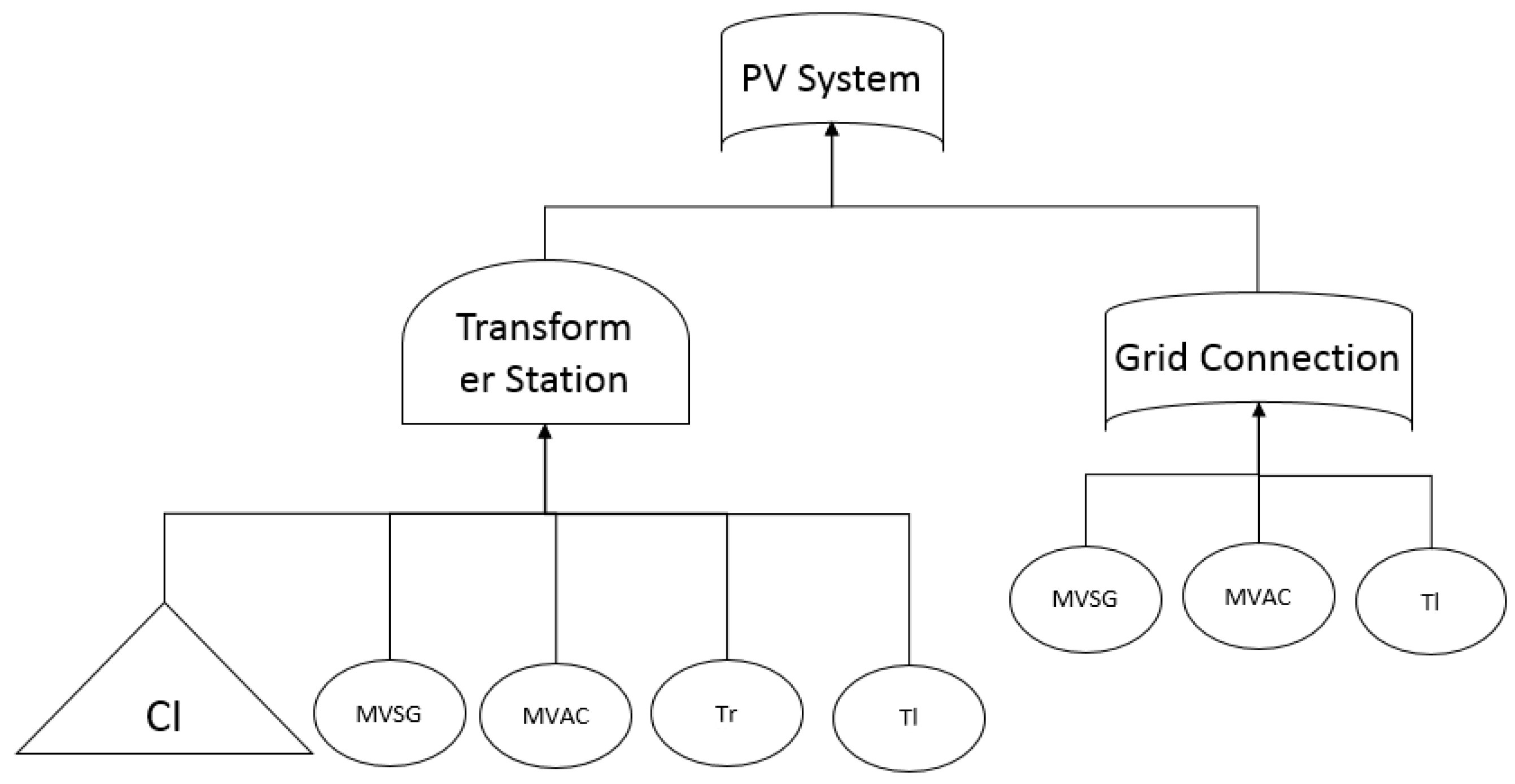
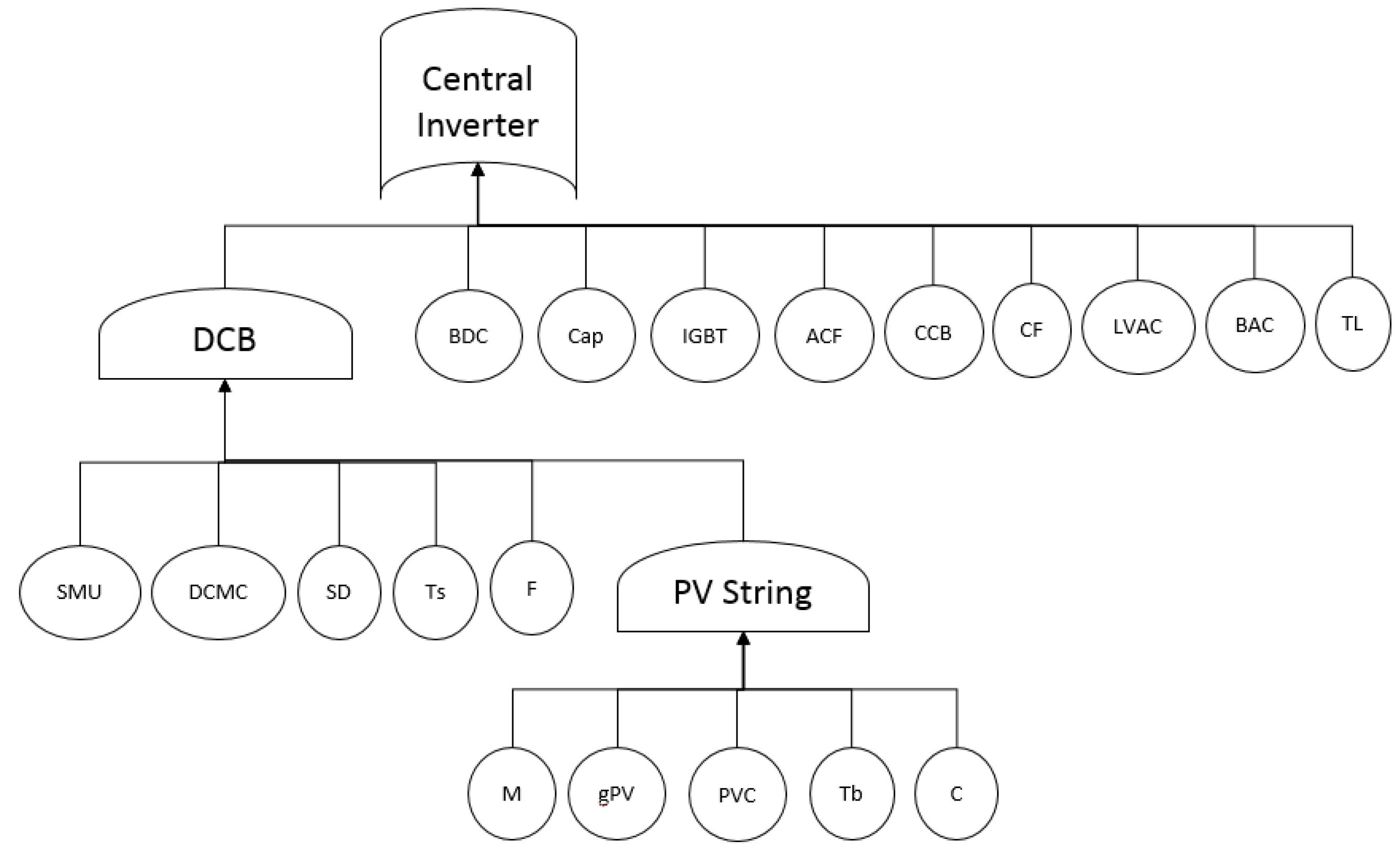
The impact of a component failure on the PV system is demonstrated here by using two fault tree diagrams that comprise different gate symbols (AND, OR and transfer) as in [17]. The fault tree diagrams are shown in Figure 1 for the (CI) PV System as a whole and Figure 2 for the PV Generator/DC side of the PV system. The corresponding subsystems are grouped into the functional blocks of PV string, DC combiner box (DCB), CI, transformer station and grid connection as are further analysed in Section 4.
The symbols for the components used in the fault tree diagrams are given in the Section of Nomenclature.
2.3. Reliability
Reliability R(t) is the ability to perform as required, without failure, for a given time interval t, under given conditions. It has an impact on the availability of the system to generate the (ideal) energy yield, namely without failures. It can be expressed mathematically as:
where λ is the (constant) failure rate. The reliability characteristics of PV system components are usually reflected using indices such as the failure rates or the Mean Time Between Failures (MTBFs).
2.4. Failure Rate and Mean Time between Failures
A failure is an unpredictably occurring event resulting in the loss of ability to meet performance requirements. The failure rate λ is the frequency of component failure. The average time a device operates without failure can be described as MTBFs. It serves as another measure of reliability for components or systems and it is equal to MTBF = 1/λ.
2.5. Failure Rates Used in This Work
Table 1 summarises the failure rates of components used here for the EL estimation. The stated values are a mixture of real system data and literature derived values. The latter was used in cases where field data was not available. Where possible, failure rates are determined from the O&M reports of existing power plants (juwi database). These values are then given in Table 1 for comparison. It was not possible to disclose details on the O&M data, as this is covered by confidentiality agreements.
2.6. Bathtub Curve
It is observed that failures in equipment, sub-systems or systems most commonly occur near the beginning and near the end of the components’ lifetime. Typically, failures of products are divided into three categories: infant- failures, midlife-failures, and wear-out-failures. This results in an overall failure occurrence typically referred to as a bathtub graph [9]. Failures of the component population are distributed over time according to a probability density function f(t). f(t) is integrated into the cumulative distribution function F(t), which statistically expresses the probability of a component to fail by time t. The reliability probability function is then expressed as R(t) = 1 − F(t).
The probability of failures with increasing lifetime is commonly represented by a Gaussian, Weibull or lognormal distribution. However, for reasons of simplicity and the lack of detailed input data such as standard deviation, shape and scale parameters, constant failure rates are assumed here. The uncertainties linked to this assumption are estimated by carrying out a sensitivity analysis.
2.7. Availability
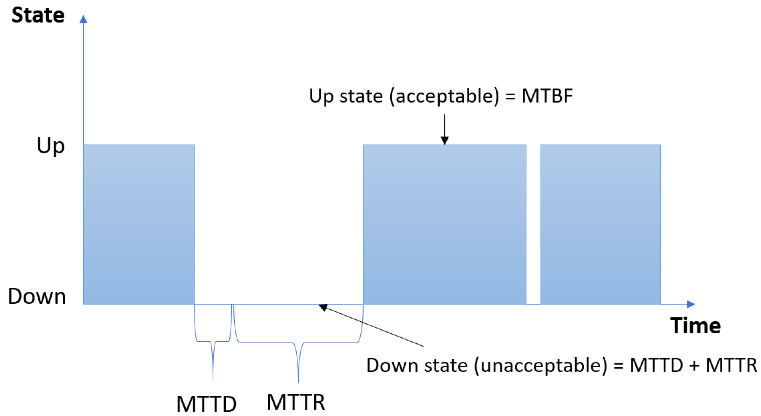
Availability (A) is defined as the percentage of time being under normal (fault-free) operation. It is the ratio of total up time divided by the total operating time and can be calculated by considering the MTBF and Mean Down time (MDT), as follows:
Figure 5 explains availability further; down state comprises the time from when a component fails to when it is available again (up state).
This includes the mean time to detect (MTTD) and the average time required to fix the failed component with all logistic aspects (mean time to repair or recover (MTTR)). If the production rate (kWhel/day) is assumed to be constant, it is convenient to extend that equation, and, instead of the percentage of time spent in each state, now the EA AE or percentage of actual production (real energy output (REO), including down times) and the ideal production (ideal energy output (IEO), fault-free) can be calculated:
EL are estimated assuming a constant daily irradiation (Yday) and a project lifetime (TLife) of 20 years as:
where, for each subsystem, ADP is the average daily production equal to the daily energy yield per installed kWp times the nominal power output, FWL is failures within lifetime and NoS is the total number of subsystems of the plant.
Failures are regarded as completely random and independent from each other (namely they do not influence each other). Thus, overall system reliability can be expressed as the product of its subsystems reliabilities. A subsystem failure rate is the sum of its components failure rates. The methods for calculating subsystem reliability from components is summarised as follows:
where RS is the reliability of the subsystem and Ri is the reliability of the component i. The same equation is valid for the overall system reliability comprising of several subsystems. System availability is similarly expressed as:
3. Subsystems Reliability
For the reliability observed in the field, all the relevant parameters used for the modelling of each subsystem are explained in the following sections. The failures of electrical components are taken from databases of juwi, where available, or relevant literature, as indicated in Table 1. The two topologies considered here are central and SI configurations.
Comparison of Central Inverter vs. Transformerless String Inverter Scheme
Assuming a typical PV string consisting of 24 PV modules of 250 WP each (approximately 30 V and 8.5 A at Standard Testing Conditions –STC), the PV string power output corresponds to 6 kWDC. The nominal power output of a CI is usually in the range of 100–900 kWAC. Thus, a CI will have a large number of strings connected in parallel (by means of DCBs). The CI concept can be divided to the following subsystems:
- PV string,
- DCB,
- CI,
- transformer,
- grid connection.
The currents of multiple strings are combined into a single pair of wires in order to carry higher currents and reduce conduction losses. These DC main cables (DCMC) are connected to the CI that converts the direct current of the PV arrays into alternating current. Further downstream, a medium voltage (MV) transformer steps up the voltage. Generated electricity is then fed into the grid.
- For the SI configuration, the modelled system has a different structure, as fewer PV strings are connected to each inverter. Multiple low voltage (LV) cables are then collected in an AC combiner box (ACB) with a D02 fuse switch disconnector (FSD) on the inverter side and an NH2 FSD on the transformer side. Thicker LV AC main cables connect the terminals with the transformer station. Assuming each ACB collects input from 10 inverters, then nine ACBs can be connected to a 1600 kVA transformer station. A PV plant that uses (transformerless) SI consists of the following subsystems:PV strings,
- string inverters,
- ACBs,
- transformer(s),
- grid connection.
The advantage of a CI scheme is the lower built cost. However, SI are more easily replaced by local electricians with shorter lead times and thus the overall impact on system yield of a failure of a single inverter becomes much less than that of a CI. One of the aims of this paper is to verify that this cost saving is also realised in the energy yield of such systems. Each subsystem is described in the next section. Several subsystems can be connected by means of bus bars, which are assumed to be failure-free.
4. Components and Subsystems for Modelling
4.1. PV String Sub-System
A string is a series connection of PV modules. It is connected to the DCB using special connectors and cables. Fuses are also inside the DCB but are considered to be part of the PV string.
4.1.1. Modules
The data used in this paper is for crystalline silicon technology modules only, as the available data is not robust enough to assess other technologies. Failure is considered to be design independent in this paper. This means it can be considered as a stochastic failure and not a systematic failure. It is assumed that systematic failures should not occur in systems with good due diligence as these would be picked up in module design qualification. Especially for modules, a systematic failure would destroy the investment, as replacing the entire array would add significant cost. This could make a project unviable and therefore any reputable energy performance contract (EPC) will ensure that only modules tested by highly ranked PV certification centres are used.
The maximum number of modules per string depends on the voltage of the individual module and the lowest temperature of the project site, as the open circuit voltage of the PV array must not exceed the upper input voltage of the inverter (as specified in the inverter manufacturer datasheet). The required parameters (nominal voltage at STC and temperature coefficients) are given on the module’s datasheet provided by the manufacturer.
4.1.2. PV Connectors and Terminals
The metallic surfaces of a connector pair are prone to thermal expansion and contraction cycles. This movement produces debris, called fretting wear. Other failure mechanisms are corrosions due to contamination and stress relaxation with increasing age. Ref. [31] reports a lifetime of 16 to 44 years (6000 to 16,000 fretting cycles) for multi-contact (MC) connectors and up to an infinite lifetime for Tyco connectors (TE Connectivity Ltd, Schaffhausen, Switzerland). The failure rate reported in [16] is also virtually negligible. Generally, it is not only a component or the material itself that may fail, but also the connections made. A poor connection can lead to arcing and fire. Therefore, terminals, creepage and clearance distances are tightly regulated. Any connection failure would most likely be due to an installation issue.
4.1.3. Fuse, Fuse Combinations, Switch Disconnectors and Circuit Breaker
The failure rates identified for these components are also given in Table 1, assuming correct sizing and mounting at operating conditions, such as fuse de-rating to account for elevated temperatures [32]. A systematic failure can be expected for inappropriate sizing, but this case is not considered here as this work focuses on failures in well-designed systems, as already mentioned.
PV DC string fuses are suitable for protecting PV modules and solar cables in reverse current situations. They should be used if the sum of the currents of parallel adjacent strings is higher than the PV module’s maximum reverse current rating, typically if there are three or more strings per DCB. Overcurrent destroys PV cells and overheats cables, which presents a considerable fire risk. The fuse will isolate the faulty strings so that the rest of the PV system can continue to generate electricity. These fuses may also cause failures if they are not carefully chosen [3].
4.1.4. Surge and Lightning Protection
Failures of surge protection devices (SPDs) also have an influence on the energy yield—for example, in case of a lightning strike, which can cause fire in the DCB. Here, they are almost seen as failure-free due to their short detection and repair times, namely if there is no lightning occurrence in the meantime, then a SPD failure will have no effect on EL.
4.1.5. Cables
In the following, it is assumed that only solar specific cables are being used, namely cables adhering to all solar specific regulations and requirements. Anything else would be considered a systematic issue and cannot be modelled purely stochastically. PV cables (PVC) need to be sized appropriately and need to withstand outdoors conditions, namely they need to be UV resistant, flame retardant and withstand high temperatures and humidity. In terms of failure rates, these can be modelled by using a Weibull distribution [33]. This is based on the physics of failure approach (failure rate as a function of electric stress and cable geometry) for the reliability of high voltage cables. In [34], failure rates for AC and DC cables are scaled according to their length, namely normalised per unit length. These rates are adopted here using the lengths given in Table 2, based on typical values found in PV installations.
4.1.6. Overall Failure Model
Each PV string (subscript S) consists of m PV modules (M), two DC PV string fuses (gPV), two PVC, two block terminal connections (Tb) and 2m + 2 PV connectors (C). The combined failure rate λS is therefore:
4.2. DC Combiner Box
A DC combiner or junction box is an enclosure or assembly in which a number of PV strings are electrically connected to a bus bar. It contains string fuses, terminal clamps, potentially a string monitoring unit (SMU) and a SPD. Furthermore, there is a DC switch disconnector (SD) in the DCB to interrupt the circuit under load (isolation) for maintenance purposes. An SPD diverts excess voltage to earth and hence provides protection from damage caused by lightning or other short-time overvoltage sources. SPDs are suitable for installation in DCBs, ACBs and inverters. The SMU allows for current measurements and detection of faulty strings.
The subsystem DCB for the reliability model consists of the SMU, a DC SD, four screw terminals (Ts) to attach the DCMC that go to the inverter and NH fuses (F). The failure rate of the subsystem DCB is given by:
4.3. Central Inverter
The inverter is one of the most vulnerable components [13,25]. Failures can occur due to fuse failure, stress, aging or damage at specific parts (faulty switches, capacitors, fans, or defective IGBT module). Insulation fault ground connection or corroded contacts are also failure modes that might result in breakdown. Failure rates for CIs are taken from [30] and complemented with field data. It can be seen from Table 1 that there is good agreement between the two sources. MTBFs vary with ambient temperature, power input and operating voltage, as discussed in [24,30]. Depending on the CI, it may be that reactive power is provided during the night to help the local power quality. In this case, the MTBF of the cooling fan (CF) and control and communication board (CCB) can be assumed to be half of the values presented.
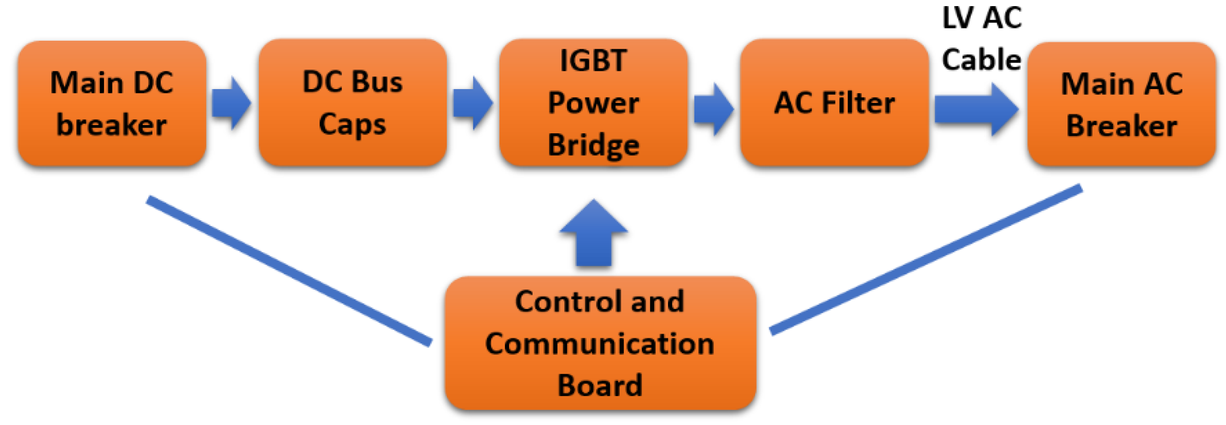
As shown in Figure 6, the CI is considered as a series network of a main DC breaker (to connect and disconnect the PV generator and inverter and to clear faults downstream, BDC), DC bus capacitors (to reduce the ripple of DC voltage, Cap), the IGBT power bridge (transforms DC to AC), an AC filter (reduces harmonics, ACF), a CCB and a CF. The LV cables (per phase, LVAC) are laid via lug terminals to the nearby transformer, where a main AC breaker (BAC) serves as a switchgear between the grid and the inverter.
For the subsystem CI, it is:
4.4. Transformer-Switchgear Station
A transformer-switchgear station comprises p LV switchgears (as part of the inverter subsystem, see above), a transformer and an MV switchgear. A switchgear is comprised of a circuit breaker with earthing switch disconnectors in order to control, protect and insolate neighbouring components. It is possible to connect various transformer stations by means of multiple MV switchgears. Requirements for transformers include that the voltage windings and AC cable set coming from the inverter must be designed for the voltages that arise from the pulsed mode of inverters. This is also valid in case SPDs are installed at the inverter side. Harmonics, voltage spikes and voltage gradient can fatigue the isolation and eventually lead to fire. The rated voltages on the low-and high-voltage windings of the transformer must be in accordance with the output voltage of the inverter and grid-connection point with a tap changer to enable alignment to the voltage level of the grid. High voltage is used to reduce transmission losses. The failure rate for the subsystem transformer (TF) is given by:
where the subscripts Tr, MVSG and MVAC represent the transformer, the MV switchgear, and the MV AC cables.
4.5. String Inverter
The subsystem SI comprises the inverter (I), an LV AC cable system, a D02 FSD inside the ACB, and the three terminals on each side of the cable. Therefore, the failure rate is given by:
4.6. AC Combiner Box
The ACB combines different LV—low current AC cables to a LV—high current conductor. This is largely used for the string inverter topology as CIs use DCBs. The failure rate of an ACB subsystem is given by:
where FSD stands for D02 FSD, Tb for block terminal, LVAC for LV AC main cable and F for NH2 fuse. Note that the three phases are split and therefore more terminals are required, which may result in higher fail.
4.7. Point of Common Coupling-Grid
The grid connection or point of common coupling (PCC) consists of a lug terminal per phase on each side, another MV switchgear and a three-phase MV AC cable system. Hence, its failure rate is given by:
5. Impact of Reliability on System Operation
Failure frequency and impact on the energy yield of a system are investigated in this section. The above equations allows for the estimation of downtime and time of failure persistence in the PV system. This can then be used to assess the potential EL using the reliability analysis as also depicted in Figure 7.
Typical MTTDs and MTTRs are given in Figure 7, which also shows the impact on system availability. The ‘fixed’ MTTDs of one day assumes a closely monitored system where data is analysed daily. In this ideal case, notifications of failures are automatically identified and so are dealt with immediately. This would be considered good practice within the industry for LSPVS and thus is a fair assumption. The MTTRs given in Figure 7 are based on field experience. Some items can theoretically be repaired sooner; however, it is often not cost-effective to arrange a maintenance visit if the impact of the failure on the system’s energy yield is marginal. A typical example would be a string sub-system failure in an LSPVS, which typically requires two visits—one to identify the fault and one to fix it. These visits will most likely be timed to coincide with scheduled maintenance, hence 90 days means that it will be repaired during the next half-yearly inspection. Assuming the repair time is five days, then the difference in EA is only 0.15%, but for a higher maintenance cost.
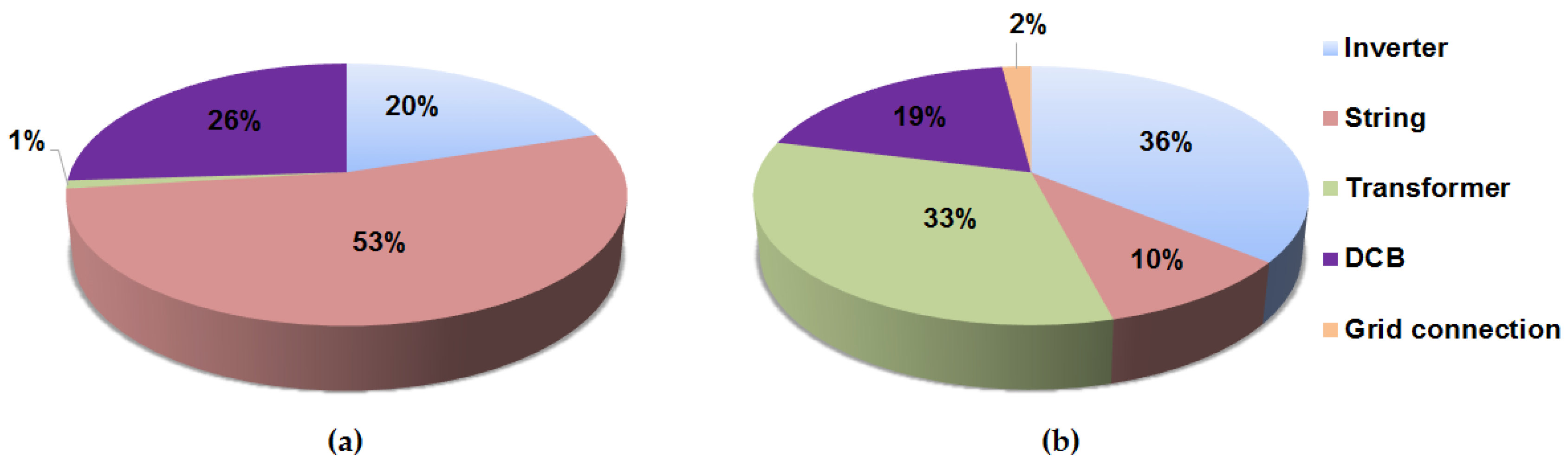
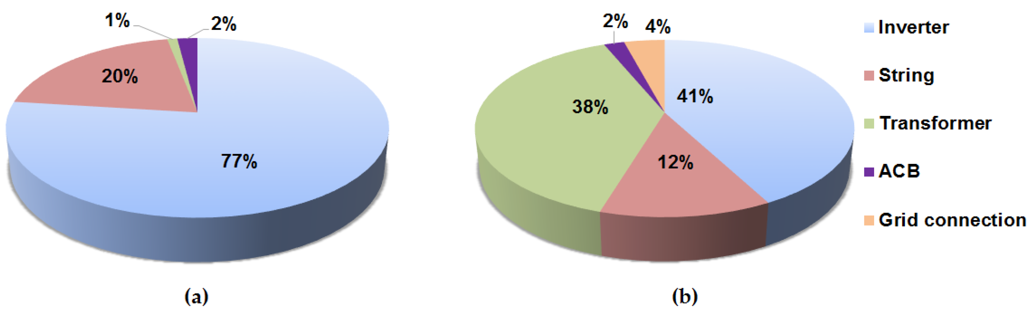
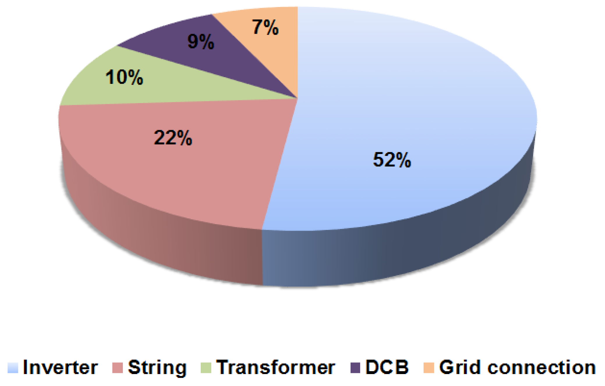
Total EA is 98.37% and 99.07% for the CI and the SI scenarios, respectively. The distribution of failures and their contribution to overall energy yield is shown in Figure 8 for the CI system and Figure 9 for the string inverter scheme. Inverter failures contribute the most to EL although the majority of failures occurs in the string subsystem. The second biggest contribution to the EA is the transformer. The overall number of occurrences is very low (only 1%), but their impact on EL is significant and the MTTR is relatively high.
Comparing Figure 8 and Figure 9 in terms of failure rates, it is apparent that the string inverter has a much higher failure likelihood than those of the actual string. Thus, string failures are reduced. This is due to the inverter taking up some of the DCB functions in terms of monitoring and fusing. The joint string and inverter loss is comparable and, as stated above, the overall EA is higher for this scenario.
There are obviously some uncertainties in the given failure rates, but the methodology given above should be a tool to evaluate the value of component reliability in LSPVS. Some items in Table 1 exhibit a broad range of reported failure rates. For instance, the MTBF for PV modules range between 218 and 16,386 years. This change would have a dramatic effect reducing the EA from around 98.4% to 95.5% at a standard repair time of 90 days (=average time between half year inspection).
The magnitude of failure rates for string fuses also varies significantly between 0.02 × 10⁻⁶/h and 5.71 × 10⁻⁶/h. This change would have a relatively small impact on EA (98.38% down to 97.14% at a higher failure rate).
The reliability of a string inverter is given between 8 (older devices) and 25 years (state-of-the-art inverters). This improvement of technology due to learning curve effects reduces the frequency of failures by 65.7% and improves AE from 98.88 to 99.13%. Device-to-device variations are also expected; however, the database currently available is not extensive enough to draw reliable conclusions on this distribution. Other components exhibit a similar range of published reliability figures but contribute less to the overall EA of the system. As an example, a decrease of AC and DC circuit breakers’ MTBF from 41 to 28 years would reduce the energy production by 0.03% only.
It was seen that replacing screw terminals with lug terminals reduced failure rates by a factor of 600. This modification can improve total energy production by 0.04% but also reduces fire risks considerably and at low additional cost. If the block terminals in the string inverter (λ = 14.6 × 10⁻⁹/h) scenario were replaced in the inverter and ACB subsystems with terminals lugs (λ = 1 × 10⁻⁹/h), there would be no noticeable increase in energy yield.
Decreasing MTTR for inverters and transformers is the most efficient way to increase EA in both scenarios. The long repair times in the case of the transformer have to do with the lead times of components. The only realistic option in reducing repair times would be to extensively monitor these components and develop a methodology to predict failures. This must identify early signs of failure so that a ‘predictive repair’ can be scheduled, eliminating downtime as much as possible. Another option would be to have replacement inverters (string scenario) in stock and a regional electrician who would visit on short notice. Combined with contractual obligations to the suppliers, the ambitious targets for MTTR would be five days for the transformer and three days for the inverter. This would increase the EA from 98.73 to 99.33%. The associated EL distribution in this pro-actively managed system is then shown in Figure 10 for a CI PV system.
Condition monitoring is shown here as a practical example of how the proposed model can be used to improve EL in a cost-effective way and by testing different O&M strategies.
6. Conclusions
A reliability and availability analysis for LSPVSs was developed. An extensive data pool was created using combined data from literature and real data from PV systems’ operation for over 25 years. Central and string inverter schemes were considered whereby a FTA and an FMEA were employed in order to carry out the reliability analysis based on their subsystems and individual subsystem components. As opposed to existing studies, the reliabilities of the transformer and point of connection have also been considered. Using updated and more realistic data to model the impact of failures, MTTR and MTTD on the energy yield allowed an assessment of the importance of the various failure modes. It is demonstrated that it is key to consider the transformer as a point of failure as its negative impact on EA is significant. This is largely due to the relatively long MTTR and catastrophic effect on yield in case of failure. It was shown that an effective way to improve EA is to reduce the MTTR for the main contributors to EL, which are the inverters and the transformers. A possible way to achieve that would be to implement predictive repairs based on detailed condition monitoring.
Author Contributions
S.B. analysed the data, conducted the reliability analysis and led the write-up. All other co-authors contributed to the writing of the manuscript and the supervision of this work.
Acknowledgments
This work has been conducted as part of the research project ‘Joint UK-India Clean Energy Centre (JUICE)’, which is funded by the Research Councils UK (RCUK)’s Energy Programme (contract no: EP/P003605/1). The projects’ funders were not directly involved in the writing of this article.
Conflicts of Interest
The authors declare no conflict of interest.
Nomenclature
| MVSG | MV switchgear |
| MVAC | MV AC cables |
| Tr | Transformer |
| Tl | Terminal lugs |
| BDC | DC breaker |
| BAC | AC breaker |
| IGBT | IGBT switch |
| ACF | AC filter |
| CCB | Control and communication board |
| CF | Cooling fan |
| LVAC | LV AC cables |
| Cap | DC capacitor |
| SMU | String monitoring unit |
| DCMC | DC main cable |
| SD | Switch disconnector |
| Ts | Screw terminal |
| F | Fuse |
| M | (PV) module |
| gPV | DC PV string fuse |
| PVC | PV string cable |
| Tb | Block terminal |
| C | (PV) Connector |
References
- REN 21. Renewables 2017: Global Status Report. Available online: http://www.ren21.net/gsr-2017/ (accessed on 9 August 2017).
- Golnas, A. PV System Reliability: An Operator’s Perspective. IEEE J. Photovolt. 2013, 3, 416–421. [Google Scholar] [CrossRef]
- Vargas, J.P.; Goss, B.; Gottschalg, R. Large scale PV systems under non-uniform and fault conditions. Sol. Energy 2015, 116, 303–313. [Google Scholar] [CrossRef] [Green Version]
- Granata, J.E.; Miller, S.; Stein, J.S. Sandia’s Photovoltaic Reliability and Performance Model; Sandia National Laboratories (SNL-NM): Albuquerque, NM, USA, 2011; p. 6.
- Alonso, R.; Román, E.; Sanz, A.; Martínez Santos, V.E.; Ibáñez, P. Analysis of inverter-voltage influence on distributed MPPT architecture performance. IEEE Trans. Ind. Electron. 2012, 59, 3900–3907. [Google Scholar] [CrossRef]
- Smet, V.; Forest, F.; Huselstein, J.J.; Richardeau, F.; Khatir, Z.; Lefebvre, S.; Berkani, M. Ageing and failure modes of IGBT modules in high-temperature power cycling. IEEE Trans. Ind. Electron. 2011, 58, 4931–4941. [Google Scholar] [CrossRef]
- Wohlgemuth, J.H.; Cunningham, D.W.; Monus, P.; Miller, J.; Nguyen, A. Long term reliability of photovoltaic modules. In Proceedings of the 2006 IEEE 4th World Conference on Photovoltaic Energy Conversion, Waikoloa, HI, USA, 7–12 May 2006; pp. 2050–2053. [Google Scholar]
- Dhere, N.G.; Shiradkar, N.; Schneller, E.; Gade, V. The reliability of bypass diodes in PV modules. In Proceedings of the Reliability of Photovoltaic Cells, Modules, Components, and Systems VI, San Diego, CA, USA, 26–29 August 2013. [Google Scholar]
- Köntges, M.; Kurtz, S.; Packard, C.; Jahn, U.; Berger, K.A.; Kato, K.; Friesen, T.; Liu, H.; Van Iseghem, M. Review of Failures of Photovoltaic Modules; IEA-PVPS T13-01:2014; International Energy Agency: Paris, France, 2014. [Google Scholar]
- Wu, D.; Zhu, J.; Betts, T.R.; Gottschalg, R. Degradation of interfacial adhesion strength within photovoltaic mini-modules during damp-heat exposure. Prog. Photovolt. 2014, 22, 796–809. [Google Scholar] [CrossRef] [Green Version]
- Zhang, P.; Li, W.; Li, S.; Wang, Y.; Xiao, W. Reliability assessment of photovoltaic power systems: Review of current status and future perspectives. Appl. Energy 2013, 104, 822–833. [Google Scholar] [CrossRef]
- Jahn, U.; Nasse, W. Operational performance of grid-connected PV systems on buildings in Germany. Prog. Photovolt. 2004, 12, 441–448. [Google Scholar] [CrossRef]
- Perdue, M.; Gottschalg, R. Energy yields of small grid connected photovoltaic system: Effects of component reliability and maintenance. IET Renew. Power Gener. 2015, 9, 432–437. [Google Scholar] [CrossRef] [Green Version]
- Hamdy, M.A.; Beshir, M.E.; Elmasry, S.E. Reliability analysis of photovoltaic systems. Appl. Energy 1989, 33, 253–263. [Google Scholar] [CrossRef]
- Hu, R.; Mi, J.; Hu, T.; Fu, M.; Yang, P. Reliability research for PV system using BDD-based fault tree analysis. In Proceedings of the 2013 International Conference on Quality, Reliability, Risk, Maintenance, and Safety Engineering, Chengdu, China, 15–18 July 2013; pp. 359–363. [Google Scholar]
- Zini, G.; Mangeant, C.; Merten, J. Reliability of large-scale grid-connected photovoltaic systems. Renew. Energy 2011, 36, 2334–2340. [Google Scholar] [CrossRef]
- Chiacchio, F.; Famoso, F.; D’Urso, D.; Brusca, S.; Aizpurua, J.I.; Cedola, L. Dynamic performance evaluation of photovoltaic power plant by stochastic hybrid fault tree automaton model. Energies 2018, 11, 306. [Google Scholar] [CrossRef]
- Akhmedjanov, F.M. Reliability Databases: State-of-the-Art and Perspectives; Report R-1235; Risö National Laboratory: Roskilde, Denmark, 2001.
- Olalla, C.; Maksimovic, D.; Deline, C.; Martinez-Salamero, L. Impact of distributed power electronics on the lifetime and reliability of PV systems. Prog. Photovolt. 2017, 25, 821–835. [Google Scholar] [CrossRef]
- Lillo-Bravo, I.; González-Martínez, P.; Larrañeta, M.; Guasumba-Codena, J. Impact of Energy Losses Due to Failures on Photovoltaic Plant Energy Balance. Energies 2018, 11, 363. [Google Scholar] [CrossRef]
- Collins, E.; Dvorack, M.; Mahn, J.; Mundt, M.; Quintana, M. Reliability and availability analysis of a fielded photovoltaic system. In Proceedings of the 2009 34th IEEE Photovoltaic Specialists Conference (PVSC), Philadelphia, PA, USA, 7–12 June 2009. [Google Scholar]
- Ahadi, A.; Ghadimi, N.; Mirabbasi, D. Reliability assessment for components of large scale photovoltaic systems. J. Power Sources 2014, 264, 211–219. [Google Scholar] [CrossRef]
- JUWI—Passion for Renewable Energies. Available online: http://www.juwi.co.uk/ (accessed on 2 August 2017).
- Zhang, P.; Wang, Y.; Xiao, W.; Li, W. Reliability evaluation of grid-connected photovoltaic power systems. IEEE Trans. Sustain. Energy 2012, 3, 379–389. [Google Scholar] [CrossRef]
- Colli, A. Failure mode and effect analysis for photovoltaic systems. Renew. Sustain. Energy Rev. 2015, 50, 804–809. [Google Scholar] [CrossRef]
- Denson, W.; Chandler, G.; Crowell, W.; Wanner, R. Non-Electronic Parts Reliability Data; IIT Research Institute: Chicago, IL, USA, 1991. [Google Scholar]
- Department of Defense of the USA. Reliability Prediction of Electronic Equipment. 1991. Available online: https://snebulos.mit.edu/projects/reference/MIL-STD/MIL-HDBK-217F-Notice2.pdf (accessed on 3 September 2017).
- Koutroulis, E.; Blaabjerg, F. Design optimization of transformerless grid-connected PV inverters including reliability. IEEE Trans. Power Electron. 2013, 28, 325–335. [Google Scholar] [CrossRef]
- Mesić, M.; Plavšić, T. The contribution of failure analyses to transmission network maintenance preferentials. Eng. Fail. Anal. 2013, 35, 262–271. [Google Scholar] [CrossRef]
- Ma, Z.J.; Thomas, S. Reliability and maintainability in photovoltaic inverter design. In Proceedings of the Annual Reliability and Maintainability Symposium, Lake Buena Vista, FL, USA, 24–27 January 2011. [Google Scholar]
- Bahaj, A. Predicting photovoltaic connector lifetime. In Proceedings of the 3rd World Conference on Photovoltaic Energy Conversion, Osaka, Japan, 11–18 May 2003; pp. 2833–2836. [Google Scholar]
- Zehner, M.; Hartmann, M.; Weizenbeck, J.; Gratzl, T.; Weigl, T.; Mayer, B.; Wirth, G.; Krawczynski, M.; Betts, T.; Gottschalg, R.; et al. Systematic analysis of meteorological irradiation effects. In Proceedings of the 25th European Photovoltaic Solar Energy Conference Exhibition, Valencia, Spain, 6–9 September 2010; pp. 4545–4548. [Google Scholar]
- BS 5760-2:1994. Reliability of Systems, Equipment and Components. Guide to the Assessment of Reliability; British Standards Institution: London, UK, 1994. [Google Scholar]
- Charki, A.; Bigaud, D. Availability estimation of a photovoltaic system. In Proceedings of the Annual Reliability and Maintainability Symposium, Orlando, FL, USA, 28–31 January 2013; pp. 4–8. [Google Scholar]
Figure 1.
Fault tree for the central inverter (CI) PV system. CI is depicted with the transfer gate symbol (triangle) because this subsystem is shown in another fault tree model.
Figure 1.
Fault tree for the central inverter (CI) PV system. CI is depicted with the transfer gate symbol (triangle) because this subsystem is shown in another fault tree model.

Figure 2.
Fault tree of the CI (DC side).

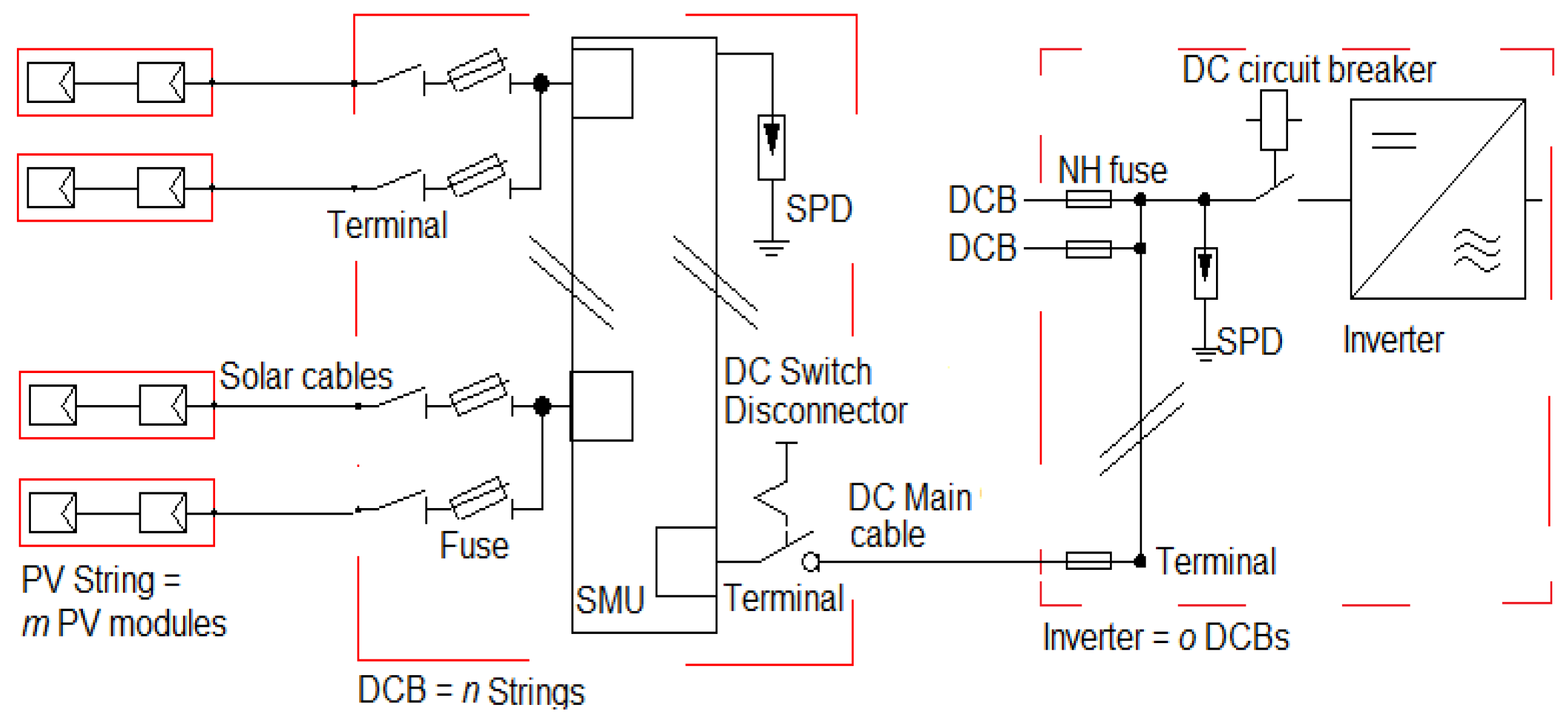
Figure 3.
Single-line diagram of the DC side of the PV plant using a CI. For the sake of simplicity, a line presents a cable system, for example two conductors for DC (+ and −). Modules are connected in series while strings are in parallel.
Figure 3.
Single-line diagram of the DC side of the PV plant using a CI. For the sake of simplicity, a line presents a cable system, for example two conductors for DC (+ and −). Modules are connected in series while strings are in parallel.

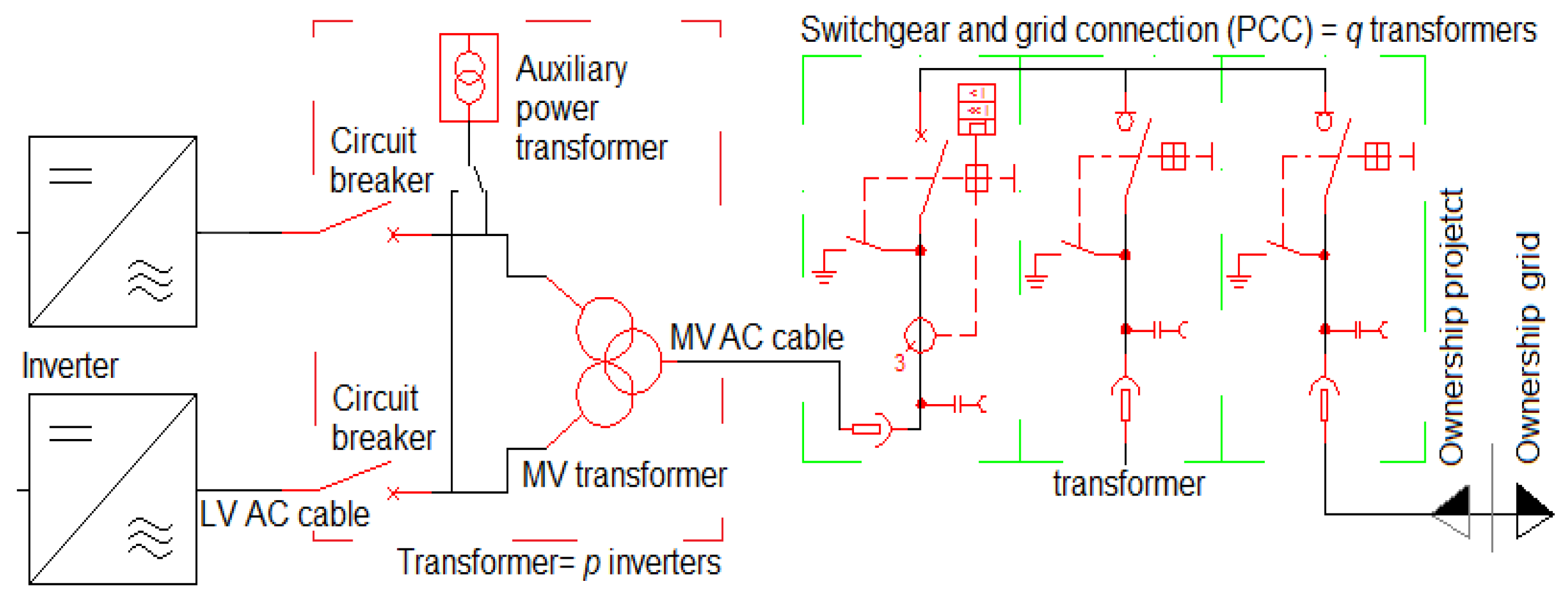
Figure 4.
Single-line diagram of the AC side of the PV plant using CIs.

Figure 5.
Representation of the availability concept.

Figure 6.
Generalized structure of inverters.

Figure 7.
Energy loss calculation model with input MTTD and MTTR (green highlighted) parameters for the subsystems.
Figure 7.
Energy loss calculation model with input MTTD and MTTR (green highlighted) parameters for the subsystems.

Figure 8.
Share of failure occurrences (a) and associated EL divided by subsystems (b) for a CI scheme.
Figure 8.
Share of failure occurrences (a) and associated EL divided by subsystems (b) for a CI scheme.

Figure 9.
Occurrences of failures per subsystem (a) share of total losses divided (b) per subsystem for the string inverter scenario.
Figure 9.
Occurrences of failures per subsystem (a) share of total losses divided (b) per subsystem for the string inverter scenario.

Figure 10.
Contribution to EL in a potential CI system where inverter and transformer repair is pro-actively managed.
Figure 10.
Contribution to EL in a potential CI system where inverter and transformer repair is pro-actively managed.


Table 1.
Failure rate λ (failures per 106 h), MTBF in years assuming 4015 h of operation per year, reliability after 20 years and literature reference for each system component (where available). [−] are extrapolated values determined from juwi’s O&M reports (as taken from different power plants). Bold figures are the selected values, which are used in this study.
| Component | Λ | MTBF | R (20y) | Ref |
|---|---|---|---|---|
| PV module | 0.0152 | 16,386 | 99.80% | [16] |
| 1.14 | 218 | 91.20% | [24] | |
| 0.025 | 9963 | 99.80% | - | |
| 0.035 | 7116 | 99.70% | - | |
| 0.04 | 6227 | 99.60% | - | |
| (Thin film) | 0.137 | 1818 | 98.90% | - |
| PV Connector | 0.00024 | 1 Mio | 100.00% | [16] |
| 0.0056 | 44,476 | 99.90% | - | |
| PV string cable | 0.002 | 124,533 | 99.60% | - |
| Terminal (lug) | 0.001 | 249,066 | 99.90% | [26] |
| -(metal sleeve) | 0.0007 | 355,809 | 99.90% | [26] |
| -(screw) | 0.603 | 413 | 95.20% | [26] |
| -(stud) | 0.0007 | 355,809 | 99.90% | [26] |
| -(block) | 0.124 | 2009 | 99.00% | [27] |
| -(block) | 0.0146 | 17,059 | 99.80% | [26] |
| -(strip) | 0.0022 | 113,212 | 99.90% | [26] |
| Fuses | 0.02 | 12,453 | 99.80% | [27] |
| String Fuse | 5.71 | 43.6 | 63.20% | [24] |
| 0.065 | 3831.8 | 99.40% | - | |
| 0.063 | 3953.4 | 99.50% | - | |
| SMU | 4.9 | 50.8 | 67.40% | - |
| 1.65 | 150.9 | 87.50% | - | |
| DC switch | 0.2 | 1245 | 98.40% | [16] |
| DC main cable | 0.0483 | 5157 | 99.60% | [28] |
| AC cable | 0.013 | 19,160 | 99.90% | [28] |
| Disconnector | 0.1 | 3558.1 | 99.40% | [29] |
| String Inverter | 18.4 | 13.5 | 22.80% | [28] |
| 12.6 | 19.8 | 36.30% | [15] | |
| 15.1 | 16.5 | 29.80% | - | |
| CI | 40.29 | 8 | 3.93% | [16] |
| 74 | 3.4 | 0.26% | - | |
| 130 | 1.9 | 0.00% | - | |
| DC Capacitor | 10.1 | 24.7 | 44.40% | [30] |
| 17.8 | 14 | 23.90% | - | |
| 41.5 | 6 | 3.57% | - | |
| DC main breaker | 8.9 | 28 | 48.90% | - |
| 6.075 | 41 | 51.10% | [30] | |
| IGBT module | 11.4 | 21.9 | 40.10% | [30] |
| 8.9 | 28 | 48.90% | - | |
| AC filter caps | 2 | 124.5 | 85.10% | [30] |
| AC circuit breaker | 5.712 | 43.6 | 63.20% | [16] |
| 2.6 | 96.2 | 81.20% | [29] | |
| 8.9 | 28 | 1.00% | ||
| 6.075 | 41 | 51.10% | - | |
| CCB | 24.9 | 10 | 13.50% | [30] |
| 26.7 | 9.3 | 11.70% | - | |
| 18.3 | 13.6 | 23.00% | [15] | |
| Cooling fan | 26.7 | 9.3 | 11.70% | - |
| Transformer | 27.4 | 9.1 | 11.10% | [30] |
| 17.8 | 14 | 23.90% | - | |
| Power switch gear | 2.01 | 123.9 | 85.00% | [29] |
| 4 | 62.3 | 72.50% | [30] |
Table 2.
Used cable lengths per cable type and inverter topology.
| Topology | Cable type | Length (m) |
|---|---|---|
| CI | Solar cables | 100 |
| DC main cables | 75 | |
| Inverter to transformer | 5 | |
| Transformer to PCC * | 100 | |
| SI | String | 70 |
| Inverter to ACB | 75 | |
| ACB to transformer | 100 | |
| Transformer to PCC | 100 |
* PCC is the point of common coupling.
© 2018 by the authors. Licensee MDPI, Basel, Switzerland. This article is an open access article distributed under the terms and conditions of the Creative Commons Attribution (CC BY) license (http://creativecommons.org/licenses/by/4.0/).
Share and Cite
MDPI and ACS Style
Baschel, S.; Koubli, E.; Roy, J.; Gottschalg, R. Impact of Component Reliability on Large Scale Photovoltaic Systems’ Performance. Energies 2018, 11, 1579. https://doi.org/10.3390/en11061579
AMA Style
Baschel S, Koubli E, Roy J, Gottschalg R. Impact of Component Reliability on Large Scale Photovoltaic Systems’ Performance. Energies. 2018; 11(6):1579. https://doi.org/10.3390/en11061579
Chicago/Turabian StyleBaschel, Stefan, Elena Koubli, Jyotirmoy Roy, and Ralph Gottschalg. 2018. "Impact of Component Reliability on Large Scale Photovoltaic Systems’ Performance" Energies 11, no. 6: 1579. https://doi.org/10.3390/en11061579
Note that from the first issue of 2016, this journal uses article numbers instead of page numbers. See further details here.