Novel Method for Identifying Fault Location of Mixed Lines

Abstract

The identification and localization of a fault are a basic requirement for optimal operation of a modern power system. An effective fault identification method significantly reduces outage time, improves the electrical supply reliability, and enhances the speed of protection control. This paper proposes a novel method based on the theory of the two-terminal traveling wave range to identify the fault location in a voltage source converter based high voltage direct current (VSC-HVDC) system containing mixed cable and overhead line segments. It uses variational mode decomposition (VMD) and the Teager energy operator (TEO) as a new method to detect the traveling wave fault through a fault signal. The effectiveness of the proposed method is verified via time domain simulation of the hybrid VSC-HVDC transmission system using PSCAD/EMTDC and MATLAB software. Simulation results show that the proposed method demonstrates high fault location accuracy and excellent robustness with a slight effect on transient resistance and fault types, and that it performs better than the existing transient detection techniques, such as wavelet transform and ensemble empirical mode decomposition.

1. Introduction

Voltage source converter based high voltage direct current (VSC-HVDC) transmission systems have many unique technical advantages. The technology is useful for the long-distance transmission of a large amount of wind power from ocean to land [1]. In addition, the use of submarine cables at sea and overhead transmission lines on land is an effective method for connecting between offshore wind farms and shore stations, which is similar to the proposed mixed-line model of this study. For such a hybrid line system of VSC-HVDC, there is a high probability of line faults occurring f due to the long-distance transmission. As a result, it is difficult to manually inspect. Therefore, achieving timely and accurate fault location identification has considerable research value.

Fault location methods for HVDC systems can be divided into the three main categories, namely, the impedance, traveling wave, and machine learning methods [2]. Of these, the traveling wave method is unaffected by fault point transition resistance, line structure, fault types, and other factors. Therefore, the traveling wave method is more applicable [3,4,5,6], it can be divided into the single-terminal traveling wave and two-terminal traveling wave methods. The double-terminal traveling wave method can more fully exploit the measured data. The single-terminal traveling wave method has difficulty in identifying the wave head, and it has lower fault ranging accuracy than the double-terminal traveling wave method for HVDC lines [7]. The traveling wave fault detection methods are mainly wavelet transform (WT), Hilbert–Huang transform (HHT), and ensemble empirical mode decomposition (EEMD). In [8,9], WT is utilized in fault locations. Choosing different wavelet based functions such as Daubechies, Morlet, and Haar, and different decomposition scales for fault location of the same model results in quite different experimental outcomes Thus, it is difficult to select a proper wavelet based function and decomposition scale when using wavelet transform for fault location. The authors in [10,11] applied the empirical mode decomposition (EMD) method to detect fault signals and then Hilbert transform is performed to locate the fault. Obviously, the fault location effect of HHT is better than that of WT. However, the HHT method cannot solve the fault location problem for all lines, such as the complex line model proposed in this study. Also, he EMD method has a few problems, such as over-enveloping and under-enveloping, modal aliasing, and serious endpoint effects [12]. In [13], first, white noise is added to the fault signal, then the mixed signal with noise is decomposed by EMD, the intrinsic mode function (IMF) component is obtained, the steps are repeated several times and finally, the average value of these IMF components is obtained. As a result, this method can offset the abnormal noise but to a certain extent it suppresses the modal aliasing phenomenon. However, these IMF components are mixed with noise, and the number of IMF components will always change. Therefore, using the normalized method makes it very difficult to eliminate the noise in the IMF component, and false modulus will occur. These disadvantages also affect the accuracy of the fault location.

In this study, a two-segment bipolar HVDC transmission line was investigated. Owing to the development of modern data acquisition (DAQ) and global positioning system (GPS) technologies, a two-terminal traveling wave method was proposed. The variational mode decomposition and Teager energy operator (VMD-TEO) were used as a novel method to detect the traveling wave fault. The VMD-TEO not only solves the difficulty in using WT to select the basic functions and decomposition scales, but also successfully suppresses the occurrence of mode aliasing during EMD in the HHT method. In addition, VMD-TEO is more accurate than EEMD in fault location.

Section 2 introduces the structure of the VSC-HVDC power transmission system and its control method. In Section 3, a novel method for the fault location identification based on the variational mode decomposition (VMD) and Teager energy operator (TEO) is developed. The simulation parameters, results, and analysis are discussed in Section 4. Finally, the conclusion is presented in Section 5.

2. VSC-HVDC Transmission System Structure and Characteristics

The double-ended VSC-HVDC transmission system is illustrated in Figure 1, which shows the main components of the voltage source converter, including a fully controlled converter bridge, direct current (DC) side capacitor, alternating current (AC) side converter transformer, and an AC filter. Among these components, the fully controlled converter bridge adopts a three-phase two-level topology, and each bridge arm comprises multiple insulated gate bipolar transistors (IGBT). The DC transmission line in the middle of the system can utilize either a cable or a transmission line. In this study, we consider a mixture of the two forms. However, for ease of analysis, the sending and receiving ends of VSC-HVDC are labeled as the M and the N sides, respectively.

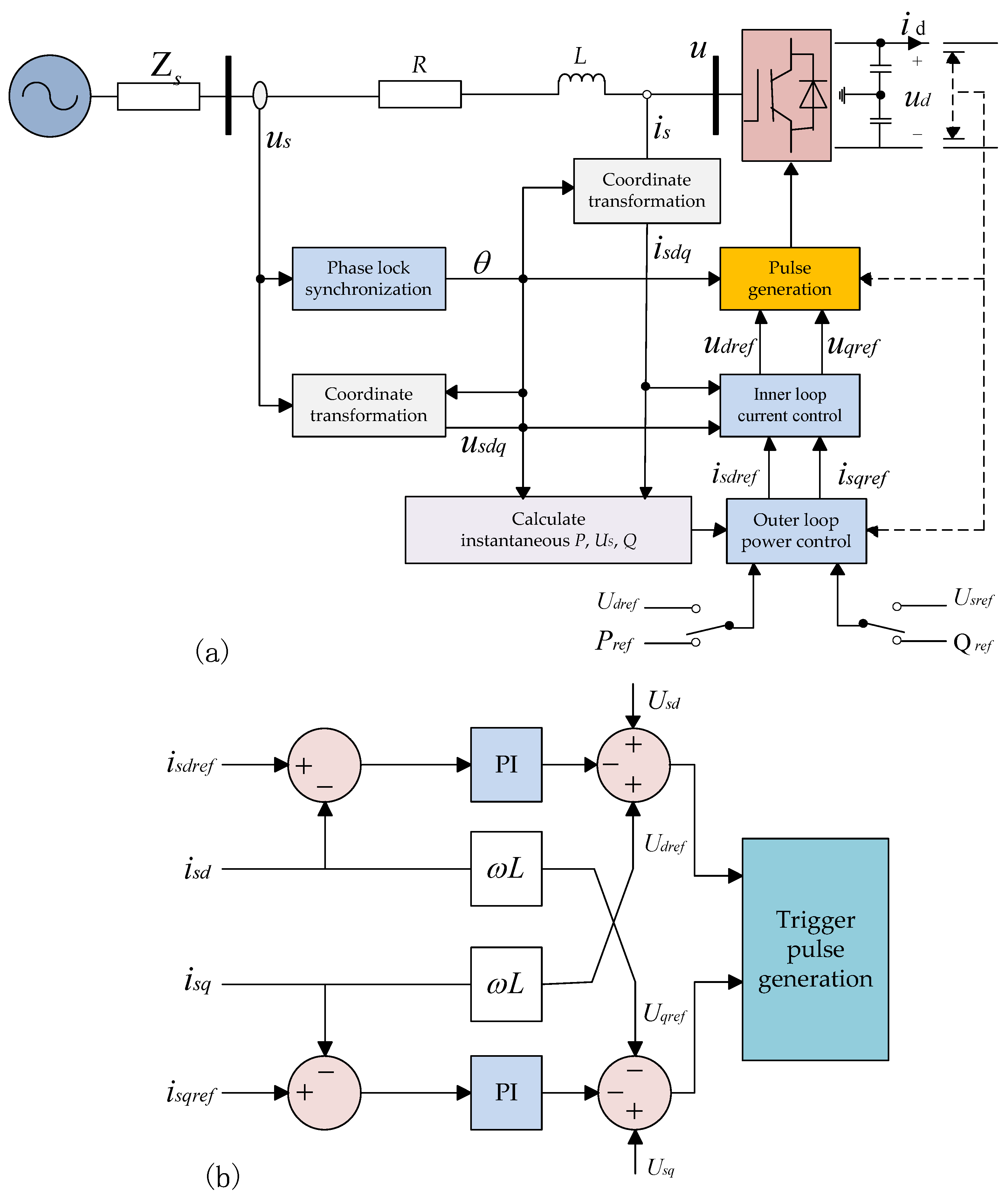
In this paper, a bipolar DC transmission line power and a current double closed-loop proportional–integral (PI) control were adopted. The VSC overall control system structure is shown in Figure 2a comprising the inner loop current controller, outer loop power regulator, phase lock synchronization, trigger pulse generation, and other components, in which the inner loop current controller is used to directly control the AC side current waveform and the phase of the converter is applied to rapidly track the reference current. The outer loop power control is based on the control objectives of the system, that is, DC voltage, active power, fixed frequency, reactive power, constant AC voltage, and other control objectives. The outer loop control mode of the M-side is constant active power control and constant reactive power control, whereas the outer loop control mode of the N-side is constant DC voltage and constant reactive power control. The inner loop controllers of the M-side and N-side are identical, and their controller structure is demonstrated in Figure 2b.

3. Mothod Analysis and Application

3.1. Theoretical Background

3.1.1. Variational Mode Decomposition (VMD)

VMD is a new signal processing method proposed by the authors of [14]. This method eliminates the signal processing method of cyclic sieve delamination used by EMD and local mean decomposition (LMD) when IMF components are obtained. This method transfers the signal decomposition process into the variational framework and iteratively searches for the optimal solution of the variational model to determine each component of the frequency center and bandwidth. VMD can be adapted to achieve frequency domain signal segmentation and effective separation of the components from the local characteristics of the data, thereby indicating improved noise robustness with a favorable sampling effect [15]. In research on traveling wave extraction of transmission line fault, the results of the VMD algorithm well reflect the singularity characteristics of the signal. The core idea of VMD is variational problems, including constructing and solving variational constraints, such as classical Wiener filtering, Hilbert transform, and frequency mixing; these constraints are described in detail in [14]. This study focuses on constructing and solving variational problems.

Construction of Variational Problems

The construction of VMD variational problems involves decomposing the original signal f into the IMF, which is expressed as Kth of modal function u_k(t), where each mode has a finite bandwidth with a center frequency in which the sum of the estimated bandwidths for each modality is minimized. For this problem, it can be expressed by the following steps:

Step 1: The analytic signal of each modal function u_k(t) is obtained by Hilbert transform and its unilateral spectrum can be calculated as follows:

$$\left(\mathsf{\delta }(t)+\frac{j}{\mathsf{\pi }t}\right)\ast u_k(t)$$

(1)

where * denotes the convolution.

Step 2: The spectrum of each modal is modulated to the corresponding baseband by combining the estimated center frequencies as follows:

$$\left(\left(\mathsf{\delta }(t)+\frac{j}{\mathsf{\pi }t}\right)\ast u_k(t)\right)e^{-j{\mathsf{\omega }}_{k}t}$$

(2)

Step 3: The norm of squared L² of the preceding demodulated signal gradient is calculated to estimate the bandwidth of each modal signal. The constrained variational problem is expressed as follows:

$$\{\begin{array}{l}\underset{\{u_k\},\{{\mathsf{\omega }}_k\}}{\min }\left({{\displaystyle \sum _k\Vert {\partial }_t\left((\mathsf{\delta }(t)+\frac{j}{\mathsf{\pi }t})\ast u_k(t)\right)e^{-j{\mathsf{\omega }}_{k}t}\Vert }}_2^2\right)\\ \mathrm{s}.\mathrm{t}.{\displaystyle \sum _k{u}_k=f}\end{array}$$

(3)

where {u_k} = {u₁, …, u_k} represents the decomposition of Kth IMF components, and {ω_k} = {ω₁, …, ω_k} represents the frequency center of each component.

Solution of the Variational Problem

The quadratic penalty factor α and Lagrange multiplication operator λ(t) are introduced to transform the constrained variational problem into an unconstrained variational problem. The augmented Lagrangian function is expressed as follows:

$$L(\{u_k\},\{{\mathsf{\omega }}_k\},\mathsf{\lambda })=\mathsf{\alpha }{{\displaystyle \sum _k\Vert {\partial }_t\left(\left(\mathsf{\delta }(t)+\frac{j}{\mathsf{\pi }t}\right)\ast u_k(t)\right)e^{-j{\mathsf{\omega }}_{k}t}\Vert }}_2^2+{\Vert f(t)-{\displaystyle \sum _k{u}_k(t)}\Vert }_2^2+\left(\mathsf{\lambda }(t),f(t)-{\displaystyle \sum _k{u}_k(t)}\right)$$

(4)

The saddle point of the preceding augmented Lagrange function is obtained through the alternating direction method of multipliers (ADMM) [16,17], which is the optimal solution of the constrained variational model of Equation (4). The ADMM optimization concept for VMD is to update u_k, ω_k and λ. The update of u_k denotes solving the following equivalent minimization problem:

$$u_k^{n+1}=\underset{u_k\in X}{\arg \min }\left(\mathsf{\alpha }{\Vert {\partial }_t\left(\left(\mathsf{\delta }(t)+\frac{j}{\mathsf{\pi }t}\right)\ast u_k(t)\right)e^{-j{\mathsf{\omega }}_{k}t}\Vert }_2^2+{\Vert f(t)-{\displaystyle \sum _i{u}_i(t)+\frac{\mathsf{\lambda }(t)}{2}}\Vert }_2^2\right)$$

(5)

This problem can be solved in a spectral domain by utilizing the Parseval/Plancherel Fourier isometry under the L² norm.

$${\widehat{u}}_k^{n+1}=\underset{{\widehat{u}}_k,u_k\in X}{\arg \min }\left(\mathsf{\alpha }{\Vert j\mathsf{\omega }[(1+\mathrm{sgn}(\mathsf{\omega }+{\mathsf{\omega }}_k)){\widehat{u}}_k(\mathsf{\omega }+{\mathsf{\omega }}_k)]\Vert }_2^2+{\Vert \widehat{f}(\mathsf{\omega })-{\displaystyle \sum _i{\widehat{u}}_i(\mathsf{\omega })+\frac{\widehat{\mathsf{\lambda }}(\mathsf{\omega })}{2}}\Vert }_2^2\right)$$

(6)

If ω is replaced by (ω − ω_k), then both terms of the above equation are written as half-space integrals over the non-negative frequencies.

$${\widehat{u}}_k^{n+1}=\underset{{\widehat{u}}_k,u_k\in X}{\arg \min }\left({\displaystyle {\int }_0^{\infty }4}\mathsf{\alpha }{(\mathsf{\omega }-{\mathsf{\omega }}_k)}^2|{\widehat{u}}_k(\mathsf{\omega }){|}^2+2{\left|\widehat{f}(\mathsf{\omega })-{\displaystyle \sum _i{\widehat{u}}_i(\mathsf{\omega })+\frac{\widehat{\mathsf{\lambda }}(\mathsf{\omega })}{2}}\right|}^2\mathrm{d}\mathsf{\omega }\right)$$

(7)

At this point, the solution of this quadratic optimization problem is

$${\widehat{u}}_k^{n+1}(\mathsf{\omega })=\frac{\widehat{f}(\mathsf{\omega })-{\displaystyle \sum _{i\ne k}{\widehat{u}}_i(\mathsf{\omega })+\frac{\widehat{\mathsf{\lambda }}(\mathsf{\omega })}{2}}}{1+2\mathsf{\alpha }{(\mathsf{\omega }-{\mathsf{\omega }}_k)}^2}$$

(8)

The update of ω_k indicates solving the following equivalent minimization problem:

$${\mathsf{\omega }}_k^{n+1}=\underset{{\mathsf{\omega }}_k}{\arg \min }\left({\Vert {\partial }_t[(\mathsf{\delta }(t)+\frac{j}{\mathsf{\pi }t})\ast u_k(t)]e^{-j{\mathsf{\omega }}_{k}t}\Vert }_2^2\right)$$

(9)

The optimization can occur in the Fourier domain and optimize the following equation:

$${\mathsf{\omega }}_k^{n+1}=\underset{{\mathsf{\omega }}_k}{\arg \min }\left({\displaystyle {\int }_0^{\infty }{(\mathsf{\omega }-{\mathsf{\omega }}_k)}^2|{\widehat{u}}_k(\mathsf{\omega }){|}^2\mathrm{d}}\mathsf{\omega }\right)$$

(10)

This quadratic problem is easily solved as:

$${\mathsf{\omega }}_k^{n+1}=\frac{{\displaystyle {\int }_0^{\infty }\mathsf{\omega }{\left|{\widehat{u}}_k^{n+1}(\mathsf{\omega })\right|}^2\mathrm{d}\mathsf{\omega }}}{{\displaystyle {\int }_0^{\infty }{\left|{\widehat{u}}_k^{n+1}(\mathsf{\omega })\right|}^2\mathrm{d}\mathsf{\omega }}}$$

(11)

where ${\widehat{u}}_k^{n+1}(\mathsf{\omega })$ is clearly identified as a Wiener filtering of the current residual. ${\mathsf{\omega }}_k^{n+1}$ is the barycenter of the power spectrum of the current modal function. If ${\widehat{u}}_k(\mathsf{\omega })$ is subjected to inverse Fourier transformation, then its real part is $\{u_k(t)\}$.

The original signal is decomposed into Kth narrowband IMF components. The concrete realization process is as follows:

Step 1: Initialize $\{{\widehat{u}}_k^1\}$, $\{{\mathsf{\omega }}_k^1\}$, $\{{\widehat{\mathsf{\lambda }}}^1\}$, and n.

Step 2: Execute cycle n = n + 1.

Step 3: For all ω ≥ 0, update $u_k$ as follows:

$$\begin{array}{l}{\widehat{u}}_k^{n+1}(\mathsf{\omega })\leftarrow \frac{\widehat{f}(\mathsf{\omega })-{\displaystyle \sum _{i<k}{\widehat{u}}_i^{n+1}(\mathsf{\omega })-{\displaystyle \sum _{i>k}{\widehat{u}}_i^n(\mathsf{\omega })+}\frac{{\widehat{\mathsf{\lambda }}}^n(\mathsf{\omega })}{2}}}{1+2\mathsf{\alpha }{(\mathsf{\omega }-{\mathsf{\omega }}_k^n)}^2}\\ k\in \{1,K\}\end{array}$$

(12)

Step 4: Update ω_k as follows:

$${\mathsf{\omega }}_k^{n+1}\leftarrow \frac{{\displaystyle {\int }_0^{\infty }\mathsf{\omega }{\left|{\widehat{u}}_k^{n+1}(\mathsf{\omega })\right|}^2\mathrm{d}\mathsf{\omega }}}{{\displaystyle {\int }_0^{\infty }{\left|{\widehat{u}}_k^{n+1}(\mathsf{\omega })\right|}^2\mathrm{d}\mathsf{\omega }}},k\in \{1,K\}$$

(13)

Step 5: Update λ as follows:

$${\widehat{\mathsf{\lambda }}}^{n+1}(\mathsf{\omega })\leftarrow {\widehat{\mathsf{\lambda }}}^n(\mathsf{\omega })+\tau (\widehat{f}(\mathsf{\omega })-{\displaystyle \sum _k{\widehat{u}}_k^{n+1}(\mathsf{\omega }))}$$

(14)

Step 6: Repeat Steps 2 to 5 until the following iteration stop condition is satisfied:

$${{\displaystyle \sum _k\Vert {\widehat{u}}_k^{n+1}-{\widehat{u}}_k^n\Vert }}_2^2/{\Vert {\widehat{u}}_k^n\Vert }_2^2<\epsilon$$

(15)

Step 7: End the iteration and obtain the Kth IMF components.

3.1.2. Teager Energy Operator (TEO)

TEO [18,19] is a kind of simple signal analysis algorithm that is mainly used to extract the instantaneous amplitude and frequency changes of a single-component signal, which can well reflect the singularity characteristics of the signal. Three adjacent samples of the original signal are calculated to extract the envelope, with excellent time resolution and real-time tracking of the measured signal waveform changes.

For the continuous signal f (t), the energy operator is defined as follows:

$$\mathsf{\psi }[f(t)]={\left(\frac{\mathrm{d}f(t)}{\mathrm{d}t}\right)}^2-f(t)\frac{{\mathrm{d}}^{2}f(t)}{\mathrm{d}{t}^2}$$

(16)

For the discrete signal f(n), the energy operator is defined as follows:

$$\mathsf{\psi }[f(t)]=f^2(n)-f(n+1)f(n-1)$$

(17)

TEO is a nonlinear operator that has a minimal computational workload. TEO can rapidly and accurately trace the signal change and is suitable for real-time signal detection and processing. The signal to be measured is first processed in accordance with the abovementioned feature, and then the Teager energy value of the single-component signal is calculated. The first peak on the instantaneous frequency spectrum corresponds to the moment when the initial surge wave reaches the detection point.

3.2. VMD and TEO for Fault Location

3.2.1. Fault Location Based on Traveling Wave Theory

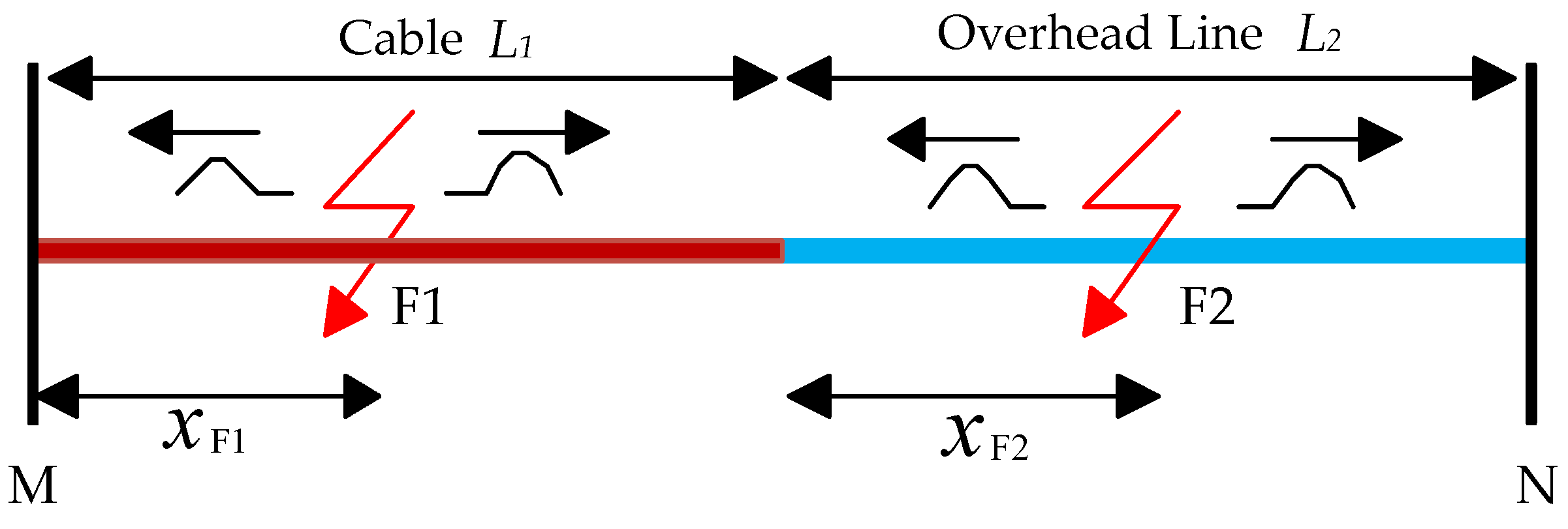
In [20], a mathematical framework based on traveling wave theory for a two-segment hybrid VSC-HVDC transmission system is proposed. The framework uses a double-ended traveling wave fault location method. In Figure 3, the fault point will produce the traveling wave at both ends, the traveling wave will reach terminal M or N, or the intersection of mixed lines will simultaneously produce reflection and refraction when the fault occurs. Assuming the traveling wave velocity on the cable is v₁, the traveling wave velocity on the overhead line is v₂.

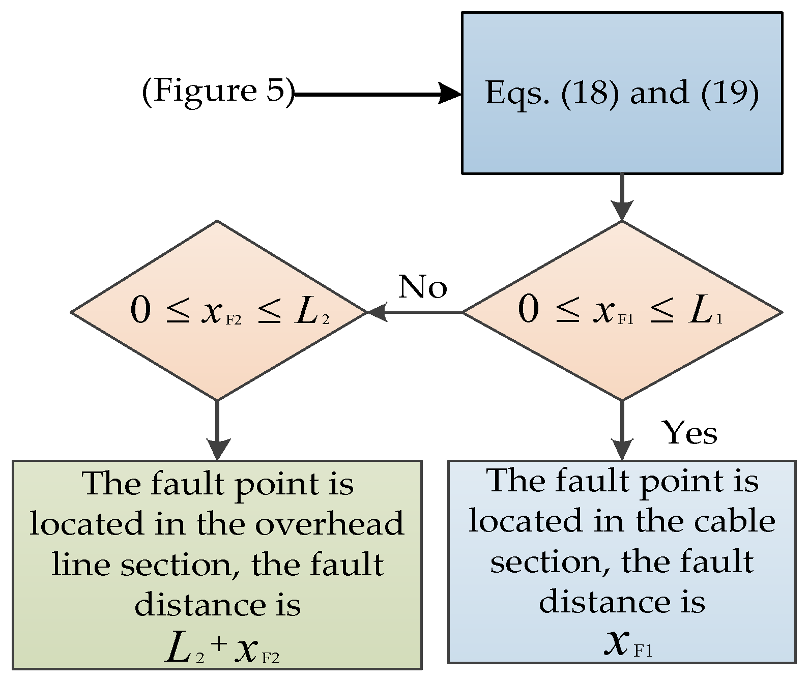
When the fault only occurs at F1 or F2, the fault distance at the cable and overhead lines can be calculated as follows:

$$x_{\mathrm{F}1}=\frac{1}{2}\left(L_1+\frac{v_1}{v_2}{L}_2-v1\Delta t\right)$$

(18)

$$x_{\mathrm{F}2}=\frac{1}{2}\left(L_2+\frac{v_2}{v_1}{L}_1-v2\Delta t\right)$$

(19)

where $x_{F1}$ is the fault distance, $x_{F2}$ is the distance from F2 to the junction of the hybrid line, and ∆t is the difference between the time when the traveling wave reaches terminals M and N.

Both terminals of the transmission line are equipped with transient recorders (TRs) and GPS signal receivers to synchronize the measurements. A communication channel such as Ethernet cables sends the synchronized measurements to a processing station. Time synchronization can be done nowadays by using GPS transducers, within a tolerance of ±1 µs [21].

The flowchart exhibited in Figure 4 is a specific algorithm for fault location. Compared to the use of the support vector machine to identify the fault zone in [22], the algorithm used in this study is relatively simple.

The VSC-HVDC transmission system with bipolar lines encounters the problem of mutual coupling, and the parameters have frequency-changing characteristics. The method of modulus analysis is considered to eliminate the influence of these factors to simplify the calculation [23]. The specific treatment method is expressed in Equation (20):

$$\left[\begin{array}{c}{i}_{m0}\\ i_{m1}\end{array}\right]=S·\left[\begin{array}{c}{i}_P\\ i_N\end{array}\right]=\frac{1}{\sqrt{2}}\left[\begin{array}{cc}1& 1\\ 1& -1\end{array}\right]·\left[\begin{array}{c}{i}_P\\ i_N\end{array}\right]$$

(20)

where i_m0 and i_m1 denote the currents of the zero-mode and one-mode traveling wave after decoupling, respectively; i_P and i_N denote the currents of the corresponding positive and negative electrodes, respectively, and S denotes the decoupling matrix.

In [24], the velocity of the one-mode traveling wave slightly changes with the frequency, whereas the velocity of the zero-mode traveling wave considerably changes with the frequency. Moreover, the velocity of the one-mode traveling wave is faster than that of the zero-mode traveling wave. Meanwhile, the modulus of the one-mode traveling wave is more stable than that of the zero-mode traveling wave, as described in [25]. Thus, the current of the one-mode traveling wave in the bipolar mode of operation should be considered to further determine the wave head to derive the time.

3.2.2. Process of Fault Location

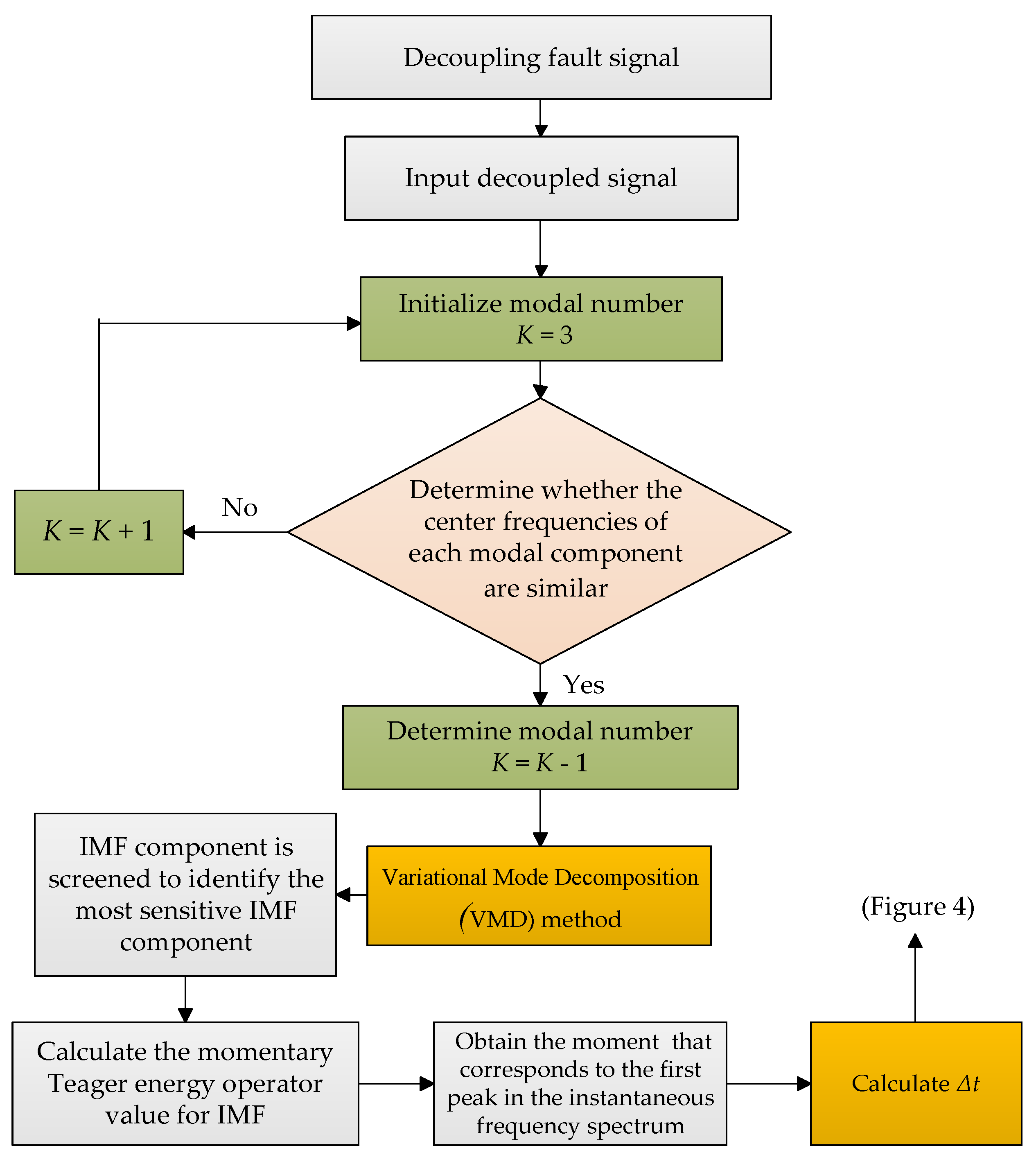
The proposed algorithm used to identify fault location of mixed lines based on VMD and TEO are demonstrated in Figure 5. The principles and details have been presented in Section 3.1 and Section 3.2 and the interpretation is as follows:

Step 1: The fault signal is extracted and performed decoupling using Equation (20).

Step 2: The decoupled fault signal is extracted, the modal number K is initialized (i.e., K = 3), and the penalty factor α and bandwidth τ are used as defaults (i.e., α = 2000, τ = 0). The reason for these parameters will be experimentally demonstrated in Section 4.

Step 3: The signal is decomposed by VMD using the parameters of Step 2, and the center frequency of each modal component is observed.

Step 4: The similarity of the center frequencies is determined. If similar, then the modal number K = K − 1 is determined; otherwise, the modal number K = K + 1. Hence, Step 3 is repeated.

Step 5: The IMF component is screened to identify the most sensitive IMF component of the fault feature.

Step 6: The momentary TEO value for the IMF is calculated in Step 5.

Step 7: The moment that corresponds to the first peak in the instantaneous frequency spectrum is obtained, which is the arrival time of the traveling wave head for the first time.

Step 8: Calculate ∆t according to the moment at which the traveling wave head arrives at both ends in Step 7.

Step 9: Calculate the fault distance according to the algorithm in Figure 4.

4. Results and Analysis

4.1. Tested Model and Related Parameters

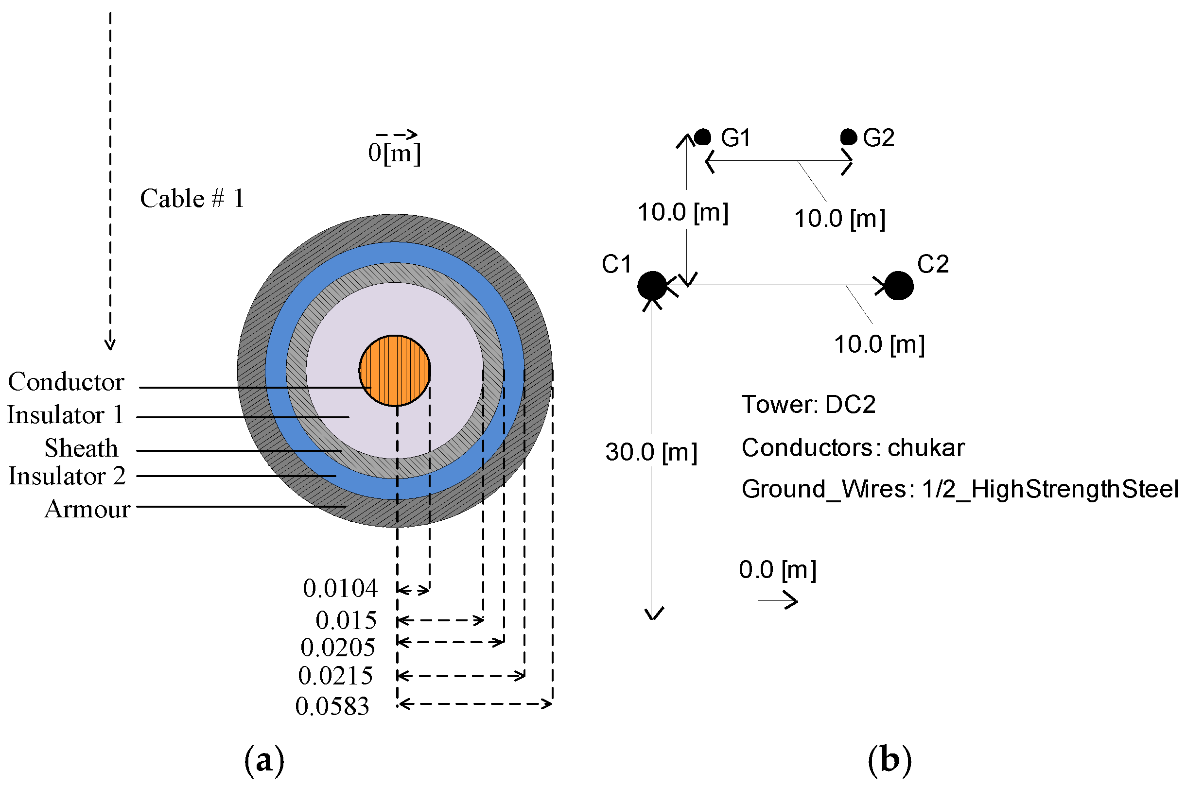
A two-segment VSC-HVDC transmission system was modeled by the simulation software PSCAD/EMTDC 4.5, Manitoba HVDC Research Centre Inc., Winnipeg, MB, Canada, and bipolar DC transmission line power and current double closed-loop PI control were adopted. The M-side system is modeled by a three-phase voltage source having main parameters, the line voltage of 110 kV, system impedance of 1.7 Ω, transformer Yn/Δ link, capacity of 25 MVA, winding voltage of 110 kV/25 kV, leakage resistance of 0.2 pu, phase reactor of 0.053 H, and equivalent resistance of 0.8 Ω. The N-side system is simulated as an infinite system by a three-phase voltage source having main parameters, the system impedance of 0 Ω, line voltage of 110 kV, transformer Yn/Δ link, capacity of 20 MVA, winding voltage of 110 kV/25 kV, leakage resistance of 0.1 pu, phase reactor of 0.053 H, and equivalent resistance 0.6 Ω. Given the frequency-dependent characteristics of the parameters, the cables and overhead lines were modeled using the frequency dependent (Phase) approach. The cable and overhead line parameters are displayed in Figure 6. The resistance, sheath resistivity, and armor resistivity of the cable are 1.72 × 10⁻⁸, 2.2 × 10⁻⁷, and 1.8 × 10⁻⁷ Ωm, respectively. The relative dielectric constant of the insulator is 2.5, and the length is 380 km. The resistance, GMR, and length of the overhead wire are 0.03206 Ω/km, 0.0122834 m, and 380 km, respectively.

4.2. Case Study

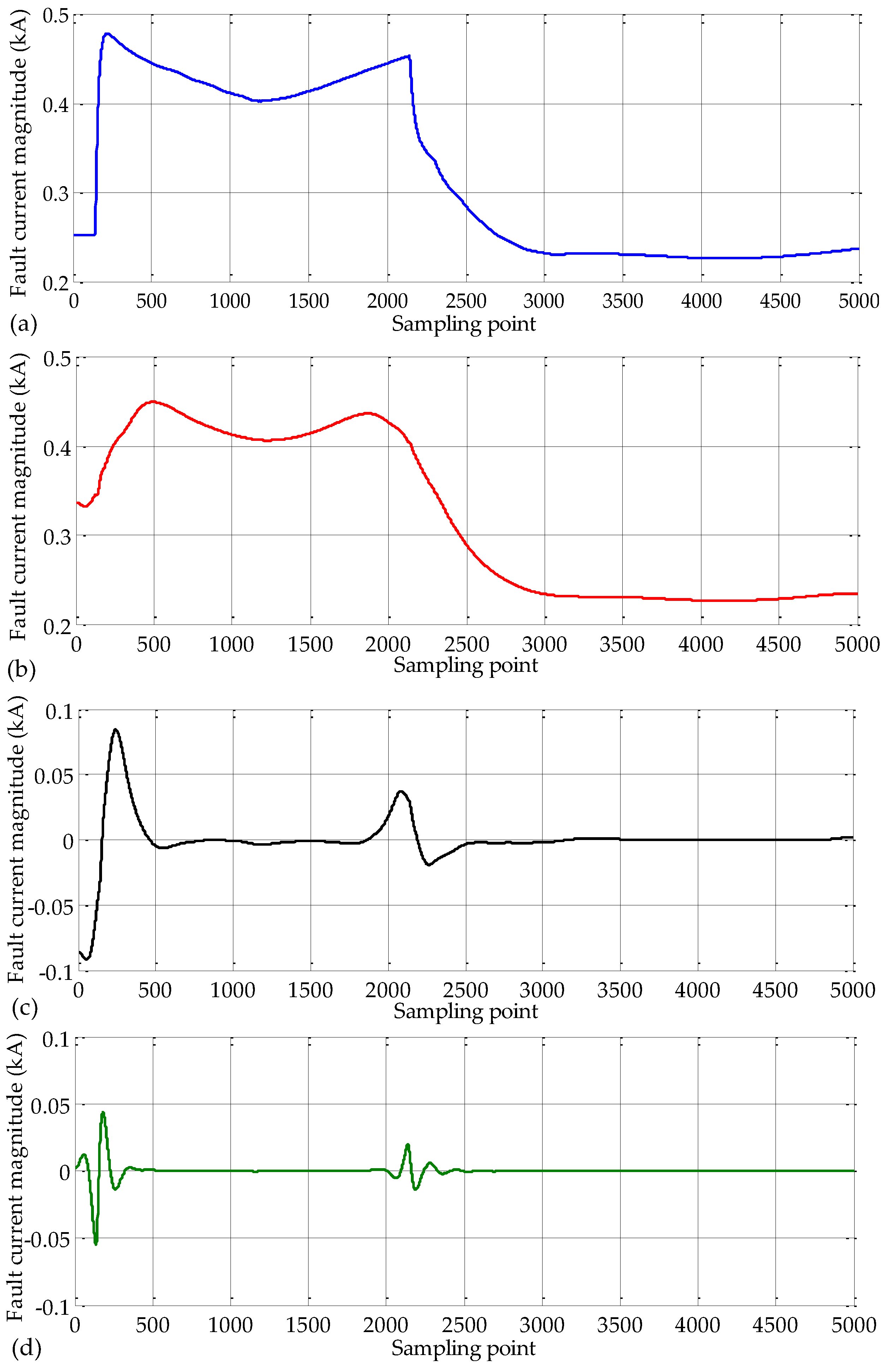
In a bipolar HVDC system, DC line faults can be positive pole to ground (PG), negative pole to ground (NG) and positive pole to negative pole (PN). Owing to the small probability of the occurrence of a bipolar ground fault, only the single-pole ground fault condition of the HVDC transmission line is described in detail. A single-phase (positive) ground fault was set at 300 km with a fault time of 2.0 s and duration of 0.02 s. After 50 ms, the fault current wave signal was analyzed, with the sampling frequency of 0.1 MHz. Such high sampling frequency could be achieved through the DAQ and GPS systems [7]. Considering the coupling between the two phases of the line, decoupling was first performed using Equation (20), and the decoupled current mode 1 components were then decomposed by VMD. The parameter settings of VMD were K = 3, α = 2000, and τ = 0. The analysis of the signal at terminal M and its VMD results, including the decoupled mode 1 current component, is presented in Figure 7. Modes 1, 2, and 3 components were decomposed by VMD.

This study indicated that the different values of K affect the modal signal waveform, and the size of the penalty factor α had a considerable influence on the decomposition result. A small value of α has led to a large bandwidth of each IMF component. However, the bandwidth of the component signal is low [26]. Taking α as 2000 and K as 2–6, the comparison of the mode 1 component in Figure 7a is illustrated in Figure 8a. Taking K as 3 and α as 500–2500, the comparison of the mode 1 component in Figure 7b is depicted in Figure 8b.

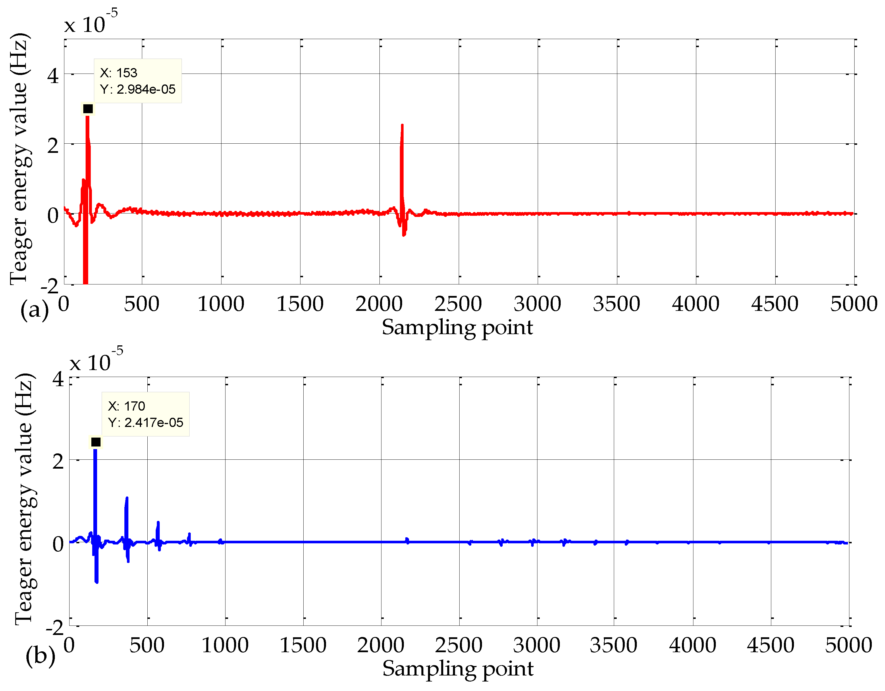
Figure 8 demonstrates that K varies from 2 to 6 when α is constant and α varies from 500 to 2500 when K is constant. Nevertheless, mode 1 remained unchanged. Therefore, the instantaneous TEO value of mode 1 was calculated. The instantaneous mode 1 energy spectrum when α = 2000 and K = 3 is exhibited in Figure 9a. In Figure 9a and the analysis in Section 3.2, the moment when the wave front of the traveling wave fault reached terminal M for the first time was t_M = 2.00153 s. The same analysis of the results of terminal N is displayed in Figure 9b, with t_N = 2.00170 s. ∆t = t_N − t_M = 0.00017 s. The two-segment line could be calculated through this method with ∆t. The next task was to determine the travel velocities v₁ and v₂ in accordance with the preceding analysis of the algorithm.

The use of an accurate traveling wave propagation speed is important to improve the accuracy of the fault location method. The most reliable method is to estimate the wave speed based on multiple sets of measurements, although the traveling wave propagation velocity can be estimated from the parameters of cables and overhead lines (v = 1/√LC, where L and C are the inductance and capacitance per unit length of the line, respectively). The specific operation is described in detail in [27]. Clearly, the propagation speed of the traveling wave could be obtained given the traveling wave arrival time and set fault distance. From multiple sets of data, the traveling wave velocity of mode 1 could be obtained as v₁ = 196,333.3333 km/s and v₂ = 293,997.1102 km/s. The value of x_F1, that is, 300.195 km, is determined by integrating v₁, v₂, and ∆t into Equation (18). Then, the theoretical calculation of the fault distance of 300.195 km can be derived from the algorithm in Figure 5. Error distance and percentage are 0.195 km and 0.065%, respectively.

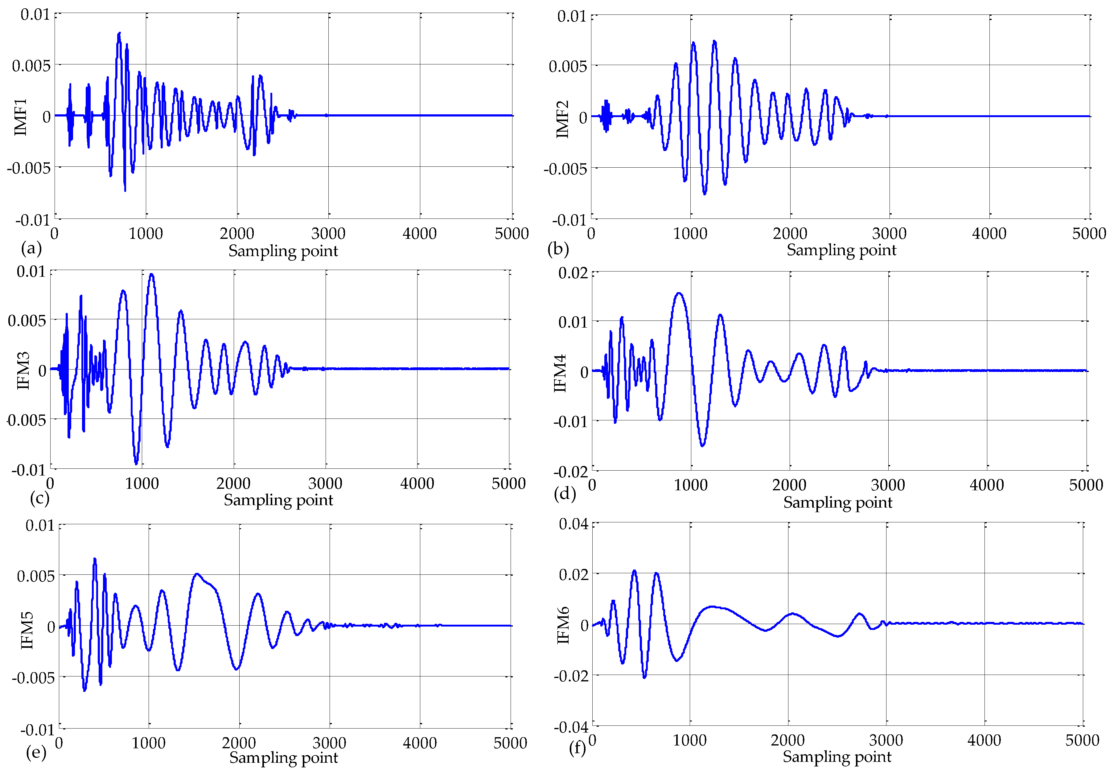
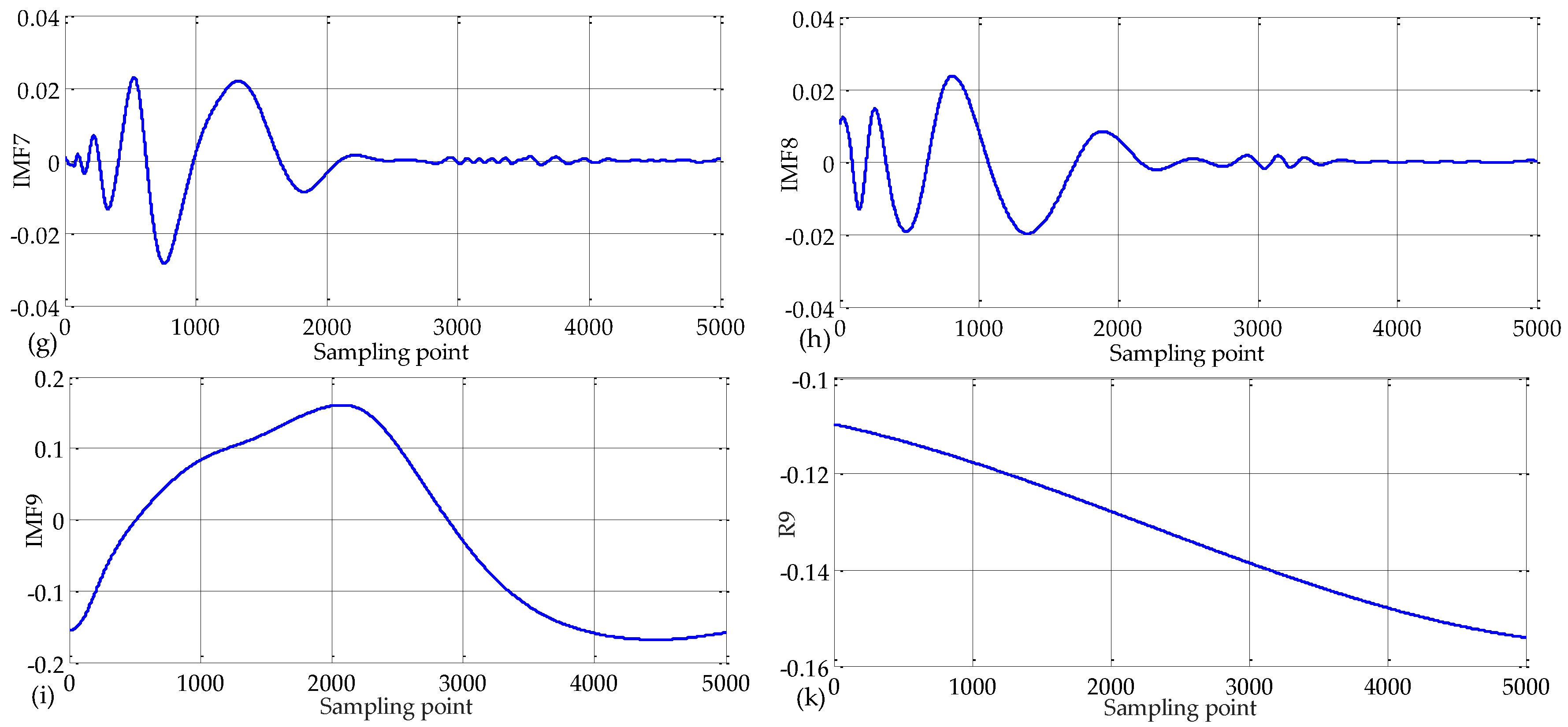
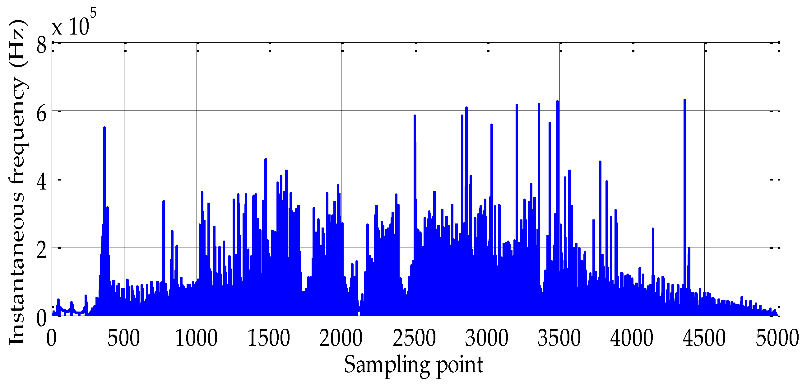
The HHT method is used to analyze the decoupled current mode 1 component. Figure 10 illustrates that the mode 1 component of the decoupled fault signal for EMD is used to obtain eight IMFs. These IMFs are arranged from high to low frequencies. R9 indicates the trend item of change, and IMF1 is a high-frequency transient component, where the Hilbert transform is performed. The instantaneous frequency is calculated to obtain the result plotted in Figure 11. A modal aliasing phenomenon is found in the EMD decomposition process of the HHT method. IMF1 is the signal itself when extreme points of the traveling wave are less than three, and the instantaneous frequency spectrum obtained by the Hilbert transformation cannot detect the time when the faulty traveling wave reaches the detection point, thereby causing the fault ranging to fail. Therefore, the HHT method cannot be used for fault location of the line model proposed in the present study.

Similarly, the EEMD method was used for analysis as a comparison. In Figure 12, the mode 1 component of the decoupled fault signal for EEMD is used to obtain the first four IMFs; the first IMF component was extracted, and its instantaneous TEO value was calculated. In Figure 13a, the moment when the wave front of the traveling wave fault reached terminal M for the first time was t = 2.00151 s. The same analysis of the results of terminal N is presented in Figure 13b, with t_N = 2.00170 s. ∆t = t_N − t_M = 0.00019 s. Similarly, the theoretical calculation of the fault distance is 299.73 km. The error distance and percentage are 0.27 km and 0.09%, respectively. Compared with the VMD method, the error distance and percentage differed by 0.075 km and 0.025%, respectively. The VMD method is clearly better than the EEMD method in terms of accuracy of fault location. The EEMD method is an improvement of the EMD. The EEMD performs EMD decomposition by adding different white noises to the mode 1 component of the decoupled fault signal multiple times and averages the results of multiple decompositions to obtain the final IMF. The EEMD, to a certain extent, suppresses the modal aliasing phenomenon. It can be seen from Figure 12 that some IMF components are mixed with noise. Through repeated EEMD decomposition experiments, we found that the number of IMF components will change. Therefore, it is very difficult to eliminate the noise in the IMF component, and there will be false modulus [28]. It was concluded that the accuracy of fault location using the EEMD method is unreliable.

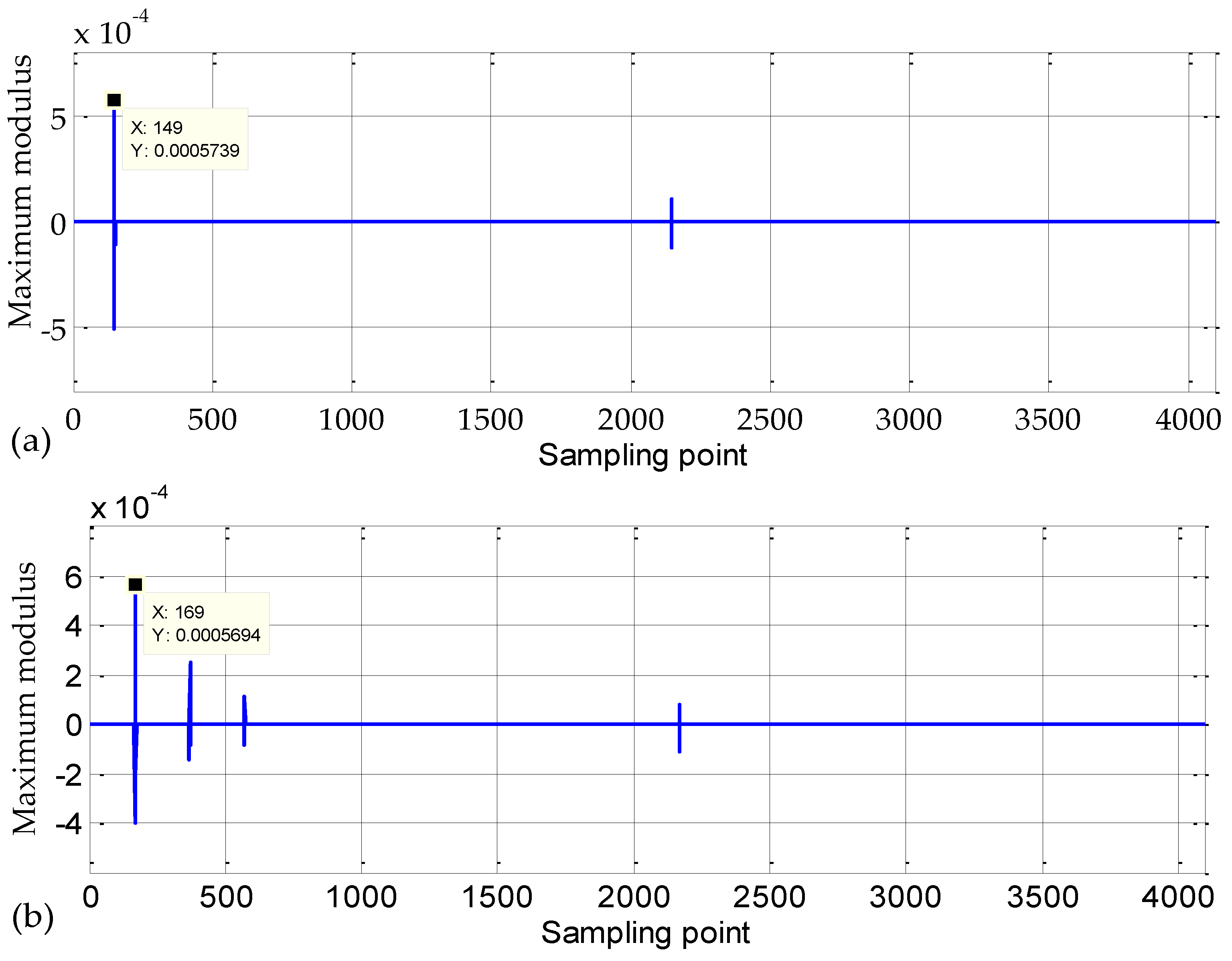
Similarly, the WT method was used for the comparison of the analysis results. The wavelet function db4 was selected to analyze the data of the first 4096 sampling points and calculate the modulus maxima of the decomposed result. In Figure 14a, the moment when the wave front of the traveling wave fault reached terminal M for the first time was t = 2.00149 s. The same analysis of the results of terminal N is illustrated in Figure 14b, with t_N = 2.00169 s. ∆t = t_N − t_M = 0.00020 s. Similarly, the theoretical calculation of the fault distance is 299.65 km. The error distance and percentage are 0.35 km and 0.117%, respectively. Compared with the VMD method, the error distance and percentage differed by 0.155 km and 0.052%, correspondingly. The VMD method is clearly better than the WT method in terms of accuracy of fault location. Currently, no unified theoretical standard is available for selecting WT basis functions and decomposition scales. The WT basis functions are frequently selected through empirical selection or comparison of different analysis results obtained from continuous experiments [27]. The error is caused by the difficulty in using WT to select the basic functions and decomposition scales. Therefore, the accuracy of fault location through the modular maxima method of the WT analysis is unreliable.

VMD and TEO were also used for fault location. According to the fault location algorithm of a two-segment line fault, the fault location results can be obtained by setting different fault points, fault grounding resistances and fault types, as shown in

Table 1. Distance measurement results of a two-segment line with different fault points and transition resistances.

Fault Location/km	Transition Resistance/Ω	Ranging Position/km	Error Distance/km	Error Percentage/%
100	0/100/200	100.19	0.19	0.19
150	0/100/200	149.77	0.23	0.153
200	0/100/200	200.33	0.33	0.165
250	0/100/200	249.68	0.32	0.128
300	0/100/200	300.195	0.195	0.065
400	0/100/200	400.54	0.54	0.135
450	0/100/200	449.72	0.28	0.062
500	0/100/200	500.56	0.56	0.112
600	0/100/200	599.49	0.51	0.085
700	0/100/200	700.58	0.58	0.083

and

Table 2. Distance measurement results of a two-segment line with different fault points and fault types.

Fault Location/km	Fault Type	Ranging Position/km	Error Distance	Fault Location/km
150	PG	149.77	0.23	0.153
	NG	149.77	0.23	0.153
	PN	149.76	0.24	0.16
250	PG	249.68	0.32	0.128
	NG	249.69	0.31	0.124
	PN	249.68	0.32	0.128
400	PG	400.54	0.54	0.135
	NG	400.54	0.54	0.135
	PN	400.54	0.54	0.135
450	PG	449.72	0.28	0.062
	NG	449.72	0.28	0.062
	PN	449.72	0.28	0.062

, respectively. Table 1 lists that the percentages of the maximum error of two-segment transmission lines for fault location and the predicted fault location are 0.19%. Table 2 shows that the accuracy of fault location is less affected by fault types.

The EEMD method is used to show that the proposed method has high accuracy in measuring distance, and the WT method is utilized to obtain the maximum modulus of two-segment line distance measurement for comparison. A comparison of the error of the fault location results of these algorithms is depicted in Figure 15. It indicates that the proposed method is more accurate than the WT and EEMD method.

5. Conclusions

In this paper, the fault location for the special mixed lines of VSC-HVDC cables and overhead lines were studied. Complexity has been added by junctions on hybrid systems, but this research object has not been thoroughly investigated before. A two-terminal traveling wave method is proposed to achieve fault location. The variational mode decomposition and Teager energy operator (VMD-TEO) is used as a novel method to detect traveling-wave arrival times. The proposed method and the existing transient detection techniques, such as the wavelet transform (WT), Hilbert–Huang transform (HHT), and ensemble empirical mode decomposition (EEMD) were used in the same experimental model set up using the simulation software PSCAD/EMTDC. The fault distance is calculated according to the principle of the two-terminal traveling wave method and the error analysis is made according to the actual fault point. The experimental results show that the proposed method performs better than other transient detection techniques. The VMD-TEO solves the difficulty in selecting the basic functions and decomposition scales in the WT method, suppresses mode aliasing occurrence during the empirical mode decomposition (EMD) in the HHT method, and solves the changes in the number of IMF and the errors caused by the false modulus in the EEMD method. The experiment conducted in this study also considered the influence of transition resistance, fault types and displayed excellent robustness.

References

- Reed, G.F.; Al Hassan, H.A.; Korytowski, M.J.; Lewis, P.T.; Grainger, B.M. Comparison of HVAC and HVDC solutions for offshore wind farms with a procedure for system economic evaluation. In Proceedings of the IEEE Energytech, Cleveland, OH, USA, 21–23 May 2013. [Google Scholar]
- Song, G.; Cai, X.; Gao, S. Survey of fault location research for HVDC transmission lines. Power Syst. Prot. Control 2012, 40, 133–137. (In Chinese) [Google Scholar]
- Hamidi, R.J.; Livani, H.; Rezaiesarlak, R. Traveling-wave detection technique using short-time matrix pencil method. IEEE Trans. Power Deliv. 2017, 32, 2565–2574. [Google Scholar]
- Lopes, F.; Dantas, K.; Silva, K.; Costa, F.B. Accurate two-terminal transmission line fault location using traveling waves. IEEE Trans. Power Deliv. 2017, 33, 873–880. [Google Scholar] [CrossRef]
- Hamidi, R.J.; Livani, H. Traveling-wave-based fault-location algorithm for hybrid multiterminal circuits. IEEE Trans. Power Deliv. 2017, 32, 135–144. [Google Scholar] [CrossRef]
- Wu, J.; Li, H.; Wang, G.; Liang, Y. An improved traveling-wave protection scheme for LCC-HVDC transmission lines. IEEE Trans. Power Deliv. 2017, 32, 106–116. [Google Scholar] [CrossRef]
- Pathirana, A.N. Travelling Wave Based DC Line Fault Location in VSC HVDC Systems. Master’s Thesis, University of Manitoba, Winnipeg, MB, Canada, 2013. [Google Scholar]
- Magnago, F.H.; Abur, A. Fault location using wavelets. IEEE Trans. Power Deliv. 1998, 13, 1475–1480. [Google Scholar] [CrossRef]
- Borghetti, A.; Bosetti, M.; Di Silvestro, M.; Nucci, C.A.; Paolone, M. Continuous-wavelet transform for fault location in distribution power networks: Definition of mother wavelets inferred from fault originated transients. IEEE Trans. Power Syst. 2008, 23, 380–388. [Google Scholar] [CrossRef]
- Bernadic, A.; Leonowicz, Z. Fault location in power networks with mixed feeders using the complex space-phasor and Hilbert–Huang transform. Electr. Power Energy. Syst. 2012, 42, 208–219. [Google Scholar] [CrossRef] [Green Version]
- Moravej, Z.; Movahhedneya, M.; Radman, G.; Pazoki, M. Effective fault location technique in three-terminal transmission line using Hilbert and discrete wavelet transform. In Proceedings of the 2015 IEEE International Conference on Electro/Information Technology (EIT), Dekalb, IL, USA, 21–23 May 2015. [Google Scholar]
- Huang, N.E. Introduction to the Hilbert Huang Transform and Its Related Mathematical Problems. In Hilbert-Huang Transform and Its Applications; World Scientific: Singapore, 2005; Volume 5, pp. 1–26. [Google Scholar]
- Liu, J.; Duan, J.; Lu, H.; Sun, Y. Fault location method based on EEMD and traveling-wave speed characteristics for HVDC transmission lines. J. Eng. Appl. Sci. 2015, 3, 106–113. [Google Scholar] [CrossRef]
- Dragomiretskiy, K.; Zosso, D. Variational Mode Decomposition. IEEE Trans. Signal Process. 2014, 62, 531–544. [Google Scholar] [CrossRef]
- Aneesh, C.; Kumar, S.; Hisham, P.M. Performance comparison of Variational Mode Decomposition over empirical Wavelet Transform for the classification of power quality disturbances using Support Vector Machine. Procedia Comput. Sci. 2015, 46, 372–380. [Google Scholar] [CrossRef]
- Rockafellar, R.T. A dual approach to solving nonlinear programming problems by unconstrained optimization. Math. Program. 1973, 5, 354–373. [Google Scholar] [CrossRef] [Green Version]
- Bertsekas, D.P. Constrained Optimization and Lagrange Multiplier Methods. Computer Science and Applied Mathematics; Academic Press: Boston, MA, USA, 1982. [Google Scholar]
- Teager, H. Some observations on oral air flow duringphonation. IEEE Trans. Acoust. Speech Signal Process. 1980, 28, 599–601. [Google Scholar] [CrossRef]
- Maragos, P.; Kaiser, J.F.; Quatieri, T.F. Energy separation in signal modulations with application to speech analysis. IEEE Trans. Signal Process. 1993, 41, 3024–3051. [Google Scholar] [CrossRef]
- Hassan, H.A.A.; Grainger, B.M.; McDermott, T.E.; Reed, G.F. Fault location identification of a hybrid HVDC-VSC system containing cable and overhead line segments using transient data. In Proceedings of the IEEE PES T&D 2016, Dallas, TX, USA, 3–5 May 2016. [Google Scholar]
- Guo, H.; Crossley, P. Design of a time synchronization system based on GPS and IEEE 1588 for transmission substations. IEEE Trans. Power Deliv. 2017, 32, 2091–2100. [Google Scholar] [CrossRef]
- Livani, H.; Evrenosoglu, C.Y. A machine learning and wavelet-based fault location method for hybrid transmission lines. IEEE Trans. Smart Grid 2014, 5, 51–59. [Google Scholar] [CrossRef]
- Song, G.; Li, D.; Chu, X. One-terminal fault location for VSC-HVDC transmission lines based on principles of parameter identification. Power Syst. Technol. 2012, 36, 94–99. (In Chinese) [Google Scholar]
- Xu, M.; Cai, Z.; Liu, Y. A novel fault location method for HVDC transmission line based on the broadband travelling wave information. Trans. China Electrotech. Soc. 2013, 28, 259–265. (In Chinese) [Google Scholar]
- Gao, S.; Suonan, J.; Song, G. Fault location method for HVDC transmission lines on the basis of the distributed parameter model. Proc. CSEE 2010, 30, 75–80. (In Chinese) [Google Scholar]
- Zhao, H.; Li, L. Fault diagnosis of wind turbine bearing based on Variational Mode Decomposition and Teager energy operator. IET Renew. Power Gener. 2017, 11, 453–460. [Google Scholar] [CrossRef]
- Nanayakkara, O.M.K.K.; Rajapakse, A.D.; Wachal, R. Location of DC line faults in conventional HVDC systems with segments of cables and overhead lines using terminal measurements. IEEE Trans. Power Deliv. 2012, 27, 279–288. [Google Scholar] [CrossRef]
- Ren, Y.; Suganthan, P.N.; Srikanth, N. A comparative study of Empirical Mode Decomposition-based short-term wind speed forecasting methods. IEEE Trans. Sustain. Energy 2015, 6, 236–244. [Google Scholar] [CrossRef]
Figure 1.
Structure of the voltage source converter based high voltage direct current (VSC-HVDC) system.
Figure 2.
Voltage source converter (VSC) control system structure: (a) Overall controller structure and (b) Inner loop controller structure.
Figure 3.
Fault occurrence at F1 and F2 at the cable and overhead lines.
Figure 4.
Algorithm for fault location of a two-segment line.
Figure 5.
Process of fault location based on variational mode decomposition (VMD) and the Teager energy operator (TEO).
Figure 6.
Parameters of HVDC transmission line: (a) cables and (b) overhead lines.
Figure 7.
Analytical signal and its VMD results at terminal M: (a) The decoupled current mode 1 component; (b) The mode 1 component; (c) The mode 2 component; and (d) The mode 3 component.
Figure 8.
The effect on the mode 1 component due to different K and α: (a) α = 2000 and K = 2–6 and (b) K = 3 and α = 500–2500.
Figure 9.
The instantaneous mode 1 energy spectrum: (a) At terminal M and (b) At terminal N.
Figure 10.
Empirical mode decomposition (EMD) results of the analytical signal at the terminal N: (a), (b), (c), (d), (e), (f), (g), (h), and (i) intrinsic mode function 1, 2, 3, 4, 5, 6, 7, 8, and 9 respectively; (k) the trend item of change of intrinsic mode function 9.
Figure 11.
Test result of the Hilbert–Huang transform (HHT) method.
Figure 12.
Ensemble empirical mode decomposition (EEMD) results of analytical signal at the terminal M: (a), (b), (c), and (d) intrinsic mode function 1, 2, 3, and 4 respectively.
Figure 13.
Intrinsic mode function 1 (IMF1) instantaneous energy spectrum: (a) At the terminal M and (b) At the terminal N.
Figure 14.
Decomposed result maximum modulus: (a) At terminal M and (b) At terminal N.
Figure 15.
Comparison of performance of different algorithms.