Strong Tracking of a H-Infinity Filter in Lithium-Ion Battery State of Charge Estimation
by
Bizhong Xia
1, 
Zheng Zhang
1,*,
Zizhou Lao
1,
Wei Wang
2,
Wei Sun
2,
Yongzhi Lai
2 and
Mingwang Wang
2 1
Graduate School at Shenzhen, Tsinghua University, Shenzhen 518055, Guangdong, China
2
Sunwoda Electronic Co. Ltd., Shenzhen 518108, Guangdong, China
*
Author to whom correspondence should be addressed.
Energies 2018, 11(6), 1481; https://doi.org/10.3390/en11061481
Submission received: 25 April 2018
/
Revised: 11 May 2018
/
Accepted: 30 May 2018
/
Published: 6 June 2018
(This article belongs to the Section D: Energy Storage and Application)
Abstract
:The accuracy of state-of-charge (SOC) estimation, one of the most important functions of a battery management system (BMS), is the basis for the proper operation of an electric vehicle. This study proposes a method for accurate SOC estimation. To achieve a balance between accuracy and simplicity, a second-order resistor–capacitor equivalent circuit model is applied before the algorithm is deduced, and the parameters of the established model are determined using a fitting technique. Battery state space equations are then described. A strong tracking H-infinity filter (STHF) is proposed based on an H-infinity filter (HF) and a strong tracking filter. By introducing a suboptimal fading factor, the STHF approach can use the relevant information in the estimation residual sequence to update the estimation results. To verify the robustness of this approach, battery test experiments are performed at different temperatures on lithium-ion batteries. Finally, the SOC estimation results obtained using the STHF suggest that the STHF method exhibits high robustness against the measured noises and initial error. For comparison, the estimation results of the commonly used extended Kalman filter (EKF) and HF methods are also displayed. It is suggested that the proposed STHF approach obtains a more accurate SOC estimation.
1. Introduction
The electric vehicle (EV) industry has rapidly developed as global energy and environment issues have been gradually aggravated. Among various types of batteries, lithium-ion batteries (LIBs) provide several advantages (e.g., high power/energy density, long lifespan, no memory effect, high operating voltage, and low self-discharge rate) [1] and are widely used in EVs. To ensure the normal operation of the entire system, a battery management system (BMS) plays an important role in an EV [2]. The system monitors and manages batteries by estimating battery states, such as the state of charge, state of energy, and state of health [3]. Accurate knowledge of the state of charge (SOC) of a battery, which refers to the residual capacity available in the battery, is a prerequisite for vehicle safety [4,5,6,7].
1.1. Definition of State of Charge
Technically, battery SOC can be defined as the ratio of the residual electricity to the nominal capacity of the battery and is expressed as follows:
where SOC(t) and SOC(t0) represent the value of SOC at time t and initial time t0 respectively. Cn denotes the nominal capacity of the battery that can be obtained from the manufacturer. iL denotes the current flowing through the voltage source and is defined to be positive during discharge and negative during charging.
Equation (1) can be rewritten in differential form:
1.2. Review of SOC Estimation Approaches
Different from voltage and current, the SOC of batteries cannot be measured directly by sensors. Several approaches have been proposed and promoted to determine the SOC of a battery [8,9,10]. The open-circuit voltage (OCV) method (also referred to as the look-up table method) exhibits high estimation accuracy; however, this technique requires a long rest time to obtain an accurate OCV, rendering it unsuitable for practical applications [11]. Ampere-hour counting is commonly used when the battery capacity is known and the load current can be obtained constantly. However, the estimation accuracy of this method is affected by the initial error and allows errors to accumulate when current measurement is inaccurate [10]. Several intelligent algorithms for SOC estimation of LIBs have recently been introduced, such as neural network [12] and fuzzy logic [13]. These methods exhibit improved robustness when batteries operate under unknown conditions. However, sizable data are required to train the network model prior to estimation, which is time-consuming [14].
In comparison with the aforementioned approaches, model-based estimation techniques are frequently studied because they can suppress unexpected disturbance and self-correct by using additional battery parameters, such as voltage [15]. The most frequently used LIB models to describe the working mechanism are the equivalent circuit model (ECM) and the electrochemical model. When a battery model is established, the SOC can be estimated using the Kalman filter (KF) method and its improved form (e.g., extended Kalman filter, unscented Kalman filter, and cubature Kalman filter) [16,17,18], particle filter [19], and the sliding mode observer (SMO) [20], among others [21]. Among these techniques, KF-based methods have been widely studied and have obtained accurate results. However, Kalman filtering operates under the assumption of zero-mean noise, which is difficult to satisfy in reality.
HF-based methods have been proved to demonstrate relatively superior robustness in battery SOC estimation. To obtain accurate estimation results, Yan et al., Zhang et al., Yan et al., and Chen et al. [22,23,24] employed the H-infinity filter in battery SOC estimation. Additionally, Rui Xiong et al. of the Beijing Institute of Technology recently provided an in-depth discussion on this approach; Lin et al. [25] introduced the linear matrix inequality-based H-infinity observer technique and proposed a multi-model probability battery SOC fusion estimation; Zhang et al. [26] applied the adaptive H-infinity method to estimate the SOC and state of energy of batteries; experimental results indicate that the adaptive H-infinity, filter-based estimator provides high estimation of battery states in real time. In Chen et al. [27], a multiscale dual H-infinity filter was proposed to estimate battery SOC and capacity in real time; the extended H-infinity filter was used in Alfi et al. [28], and the parameters required were obtained using radial basis function networks. The H-infinity filter was also used to determine the parameters of LIBs and thus improve estimation accuracy [29]. Meanwhile, the H-infinity-based nonlinear observer method was introduced for battery SOC estimation [30,31].
1.3. Contribution of This Paper
Owing to its good robustness, the H-infinity algorithm has been extensively researched for its application in battery SOC estimation, which can be derived using different analytic methods, such as game theory and transfer function approaches. By introducing a cost function J, the H-infinity filter based on game theory aims to minimize the estimation error in the worst-case scenario. Regardless, it is difficult to track the sudden state changes in the steady state. To alleviate this problem, the STHF approach to SOC estimation is proposed in this study. Through the introduction of a suboptimal fading factor to update the variance of the estimation error, the STHF algorithm obtains stronger robustness against model uncertainties and sudden noise.
To verify the SOC estimation accuracy of the STHF approach, this study establishes a second-order ECM to simulate the dynamic performance of LIBs. The parameters in the model are identified by curve fitting. The HF and STHF methods used in battery SOC estimation are then analyzed. Battery tests under different discharge conditions are performed at different temperatures. A comparison of the estimation results based on STHF and other algorithms suggests that STHF-based methods exhibit higher SOC estimation accuracy, compared with other algorithms.
1.4. Organization of This Paper
The remainder of this paper is outlined as follows: Section 2 introduces a second-order resistor–capacitor (RC) network model for LIBs and identifies the parameters. In Section 3, the strong tracking H-infinity filter algorithm is derived, and STHF-based SOC estimation is analyzed. Section 4 describes the battery test procedure in the New European Driving Cycle (NEDC), and the SOC estimation accuracy of STHF is verified. Finally, Section 5 summarizes the study.
2. Battery Model and Parameter Identification
2.1. Equivalent Circuit Model of Lithium-Ion Batteries
To obtain the accuracy of SOC estimation results, an appropriate battery model should be selected to describe the operating mechanism and external characteristics. ECMs can easily identify model parameters and provide high accuracy that can satisfy the requirements of BMS [32,33]. By employing the resistor, capacitor, and voltage source, ECMs can describe the dynamic, external characteristics of LIBs. ECMs come in various types, including the first-order RC ECM [8,13,34], second-order RC ECM [7,35], fractional-order RC ECM [20], and so on.
A higher-order ECM generally indicates higher accuracy to simulate battery characteristics; regardless, the model can be more complex and requires a stricter criterion for the BMS hardware. To strike a balance between accuracy and simplicity, a second-order ECM is used in the present study.
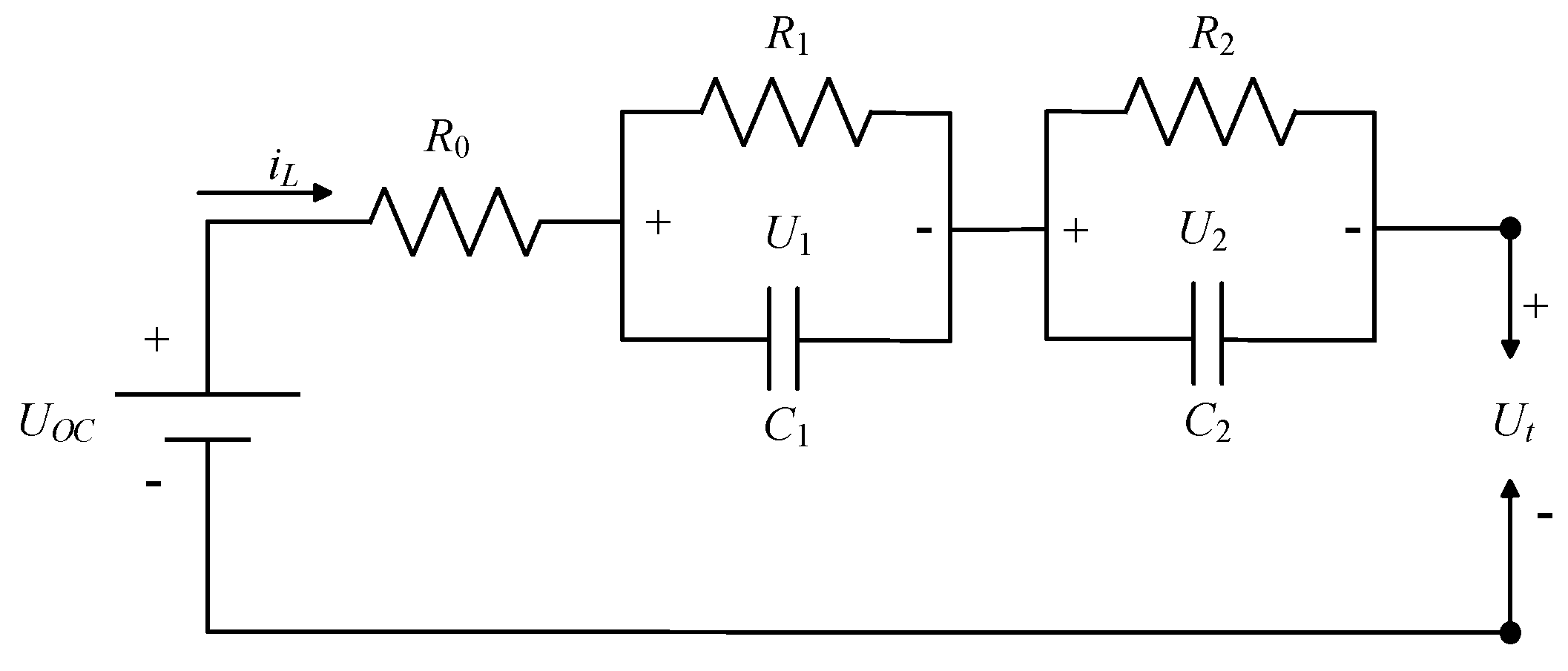
As shown in Figure 1, a typical second-order RC ECM is composed of two parallel RC circuits, one resistor and one voltage source, which are connected in series. Uoc represents the OCV of the battery, which varies nonlinearly with SOC, and the relationship between the OCV and SOC vary at different temperatures. R0 is ohmic resistance, and Ut is the terminal voltage of the battery. The first RC circuit is employed to simulate the electrochemical polarization of LIBs, and the second simulates concentration polarization. U1 and U2 represent the polarization voltages of the two RC circuits.
In accordance with Thevenin’s Theorem, the following equations can be established:
For convenience in applying the algorithm for SOC estimation, the aforementioned differential equations can be rewritten as follows:
2.2. Model Parameter Identification
Once the battery model is determined, the parameters in the model need to be identified. The parameters of the battery model change constantly as the battery ages. Online parameter identification continuously updates the estimation values of these parameters to increase the accuracy of SOC estimation. However, online methods require complexity and are beyond the scope of the study. Thus, simple offline parameter identification methods, which predetermine the parameters, are used in this study.
To calculate the model parameters, pulse discharge current experiments were conducted on a Samsung ICR18650-22P LIB (Seoul, South Korea) at 0 °C, 20 °C, and 40 °C. Essential information on this battery is listed in Table 1, and the procedure of the experiment is illustrated in Figure 2.
By applying the commonly studied exponential-function fitting technique, the model components at different temperatures can be identified, as listed in Table 2. The details regarding offline parameter identification are discussed in Xia et al. [21] and thus are not provided in this study.
Another important task is the determination of the relationship between Uoc and SOC, which varies with temperature. By means of the experiments shown in Figure 2, the OCV at different SOCs can be determined. We obtained the approximate correspondence between SOC and Uoc by the fitting function in MATLAB. To achieve a balance between accuracy and computation, a quartic polynomial was applied. The SOC–OCV nonlinear relationship curves at 0 °C, 20 °C, and 40 °C are described in Equations (6)–(8) and are shown in Figure 3.
2.3. State–Space Equation
To employ the algorithm for estimating the SOC of LIBs, the state-space equation was formulated according to Equations (2), (4) and (5). However, the equations needed to be discretized because the sensors could not continuously generate the measured values. Differently stated, the sampling time T exists. The ultimate battery model discrete state-space equation is written as
The observed equation is expressed as
3. Strong Tracking H-Infinity Filter Algorithm for SOC Estimation
3.1. SOC Estimation Based on H-Infinity Filters
As discussed in previous sections, H-infinity filters exhibit high robustness and are widely studied for state estimation. The estimation accuracy is mainly influenced by modeling errors and external noise. At time k, the assumption is that the process noise of input uk and the measurement noise of the observed value yk are wk and vk, respectively. xk denotes the system state at time k, and the discrete-time system can be expressed as
In accordance with Equations (9) and (10),
However, the SOC and OCV exhibit a nonlinear relationship; thus, Equation (10) also shows a nonlinear behavior. To solve this problem, Equation (10) can be determined according to Burgos et al. [36] as follows:
After the system equations were established, an approach based on game theory was applied and the cost function was introduced, as follows [37]:
where the tracked target denotes the SOC, and its estimated value is ; x0 represents the initial SOC, and denotes the estimation of . Four weighting matrices in Equation (16) were determined to be symmetric-positive and they were selected based on the specific problem.
denotes the norm of s, which can be calculated by
The cost function J can be viewed as a contest between nature and engineers. By introducing errors (current error Wk, voltage noise Vk, and the initial error in the denominator), nature aims to maximize the estimation error. However, appropriate methods in the numerator are preferred to minimize the estimation error. This study aimed to achieve as small a value as possible for the function J and thus obtain an accurate SOC. Nevertheless, J was difficult to be minimized directly; thus, a bound value θ that can be easily satisfied was determined. That is, we wanted to find a value for to satisfy
Equations (16) and (19) can be integrated and rewritten as
From Equations (6) and (14), the following can be derived:
where is defined as
Combining these results with Equation (15) derives
Thus, the discrete H-infinity filter can be regarded as a minimax problem; that is,
In Dan et al. [38], the author solved this problem in great detail from theory analysis to equation deduction; as such, it is not discussed in the present study. By using the Lagrange multiplier approach, x0, wk, and yk were determined when the function J had a maximum or a minimum. The aforementioned analysis indicates that, to achieve the threshold in Equation (19), SOC estimation based on the H-infinity filter is summarized in Table 3.
To ensure that the estimator can be solved, the following equation must be satisfied:
The aforementioned analysis shows that the H-infinity filter considered the worst conditions, which hardly occur in reality. Thus, the H-infinity filter showed strong robustness, compared with other algorithms. Regardless, the determination of the cost function parameters involved complexity because they varied depending on the problem.
- Threshold θ: To improve the accuracy of the estimator, 1/θ should be as small as possible. However, if the boundary conditions are extremely high, the filter error tends to increase or diverge. In consideration of the existence of battery modeling error, the threshold theta cannot be too large to avoid divergence. Therefore, the value of theta can set to 1, 10−2, 10−3, 10−4 and 10−5 respectively, and the simulation results indicate that the estimation effect is optimal when theta is 10−2. So, 1/θ is set to 100 in this paper.
- Weighting matrices: Normally, the initial estimation error and measured noise statistics cannot be predetermined in practical applications; thus, weighting matrices cannot be preset given such information. For simplicity, Sk, Wk, and Vk were set as the identity matrices, and their dimensions were determined using Equation (16). P0 was determined by the initial error.
3.2. Strong Tracking H-Infinity Filter Estimation
The fundamental theory of H-infinity was introduced in Section 3.1, and the parameters were determined. However, the HF filter is not sensitive to sudden changes in state and model uncertainties. To overcome these disadvantages, the STHF approach is proposed. In Zhou et al., He et al. and Bai et al. [39,40,41], Zhou et al. originally proposed the STF approach based on the extended Kalman filter (EKF) for nonlinear system state estimation. By employing a suboptimal fading factor, this method uses the relevant information in the estimation residual sequence, which can provide high robustness to alterations in process parameters. On the basis of the explanation in Zhou et al. [39], the suboptimal fading factor can be calculated using the following equations:
where E0,k denotes the residual sequence and is determined by
When the aforementioned variables are determined, the suboptimal fading factor λ at time k is given by
where
Note: In Equation (27), Qk is the current noise covariance, and Rk is the voltage noise covariance. In Equation (30), ρ is the forgetting factor, which can be set to 0.95 in this study. In Equation (32) tr (·) refers to the trace of a matrix.
The combination of the H-infinity filter and STF for SOC estimation is presented in Table 4.
4. Experimental Results and Discussion
4.1. Workbench
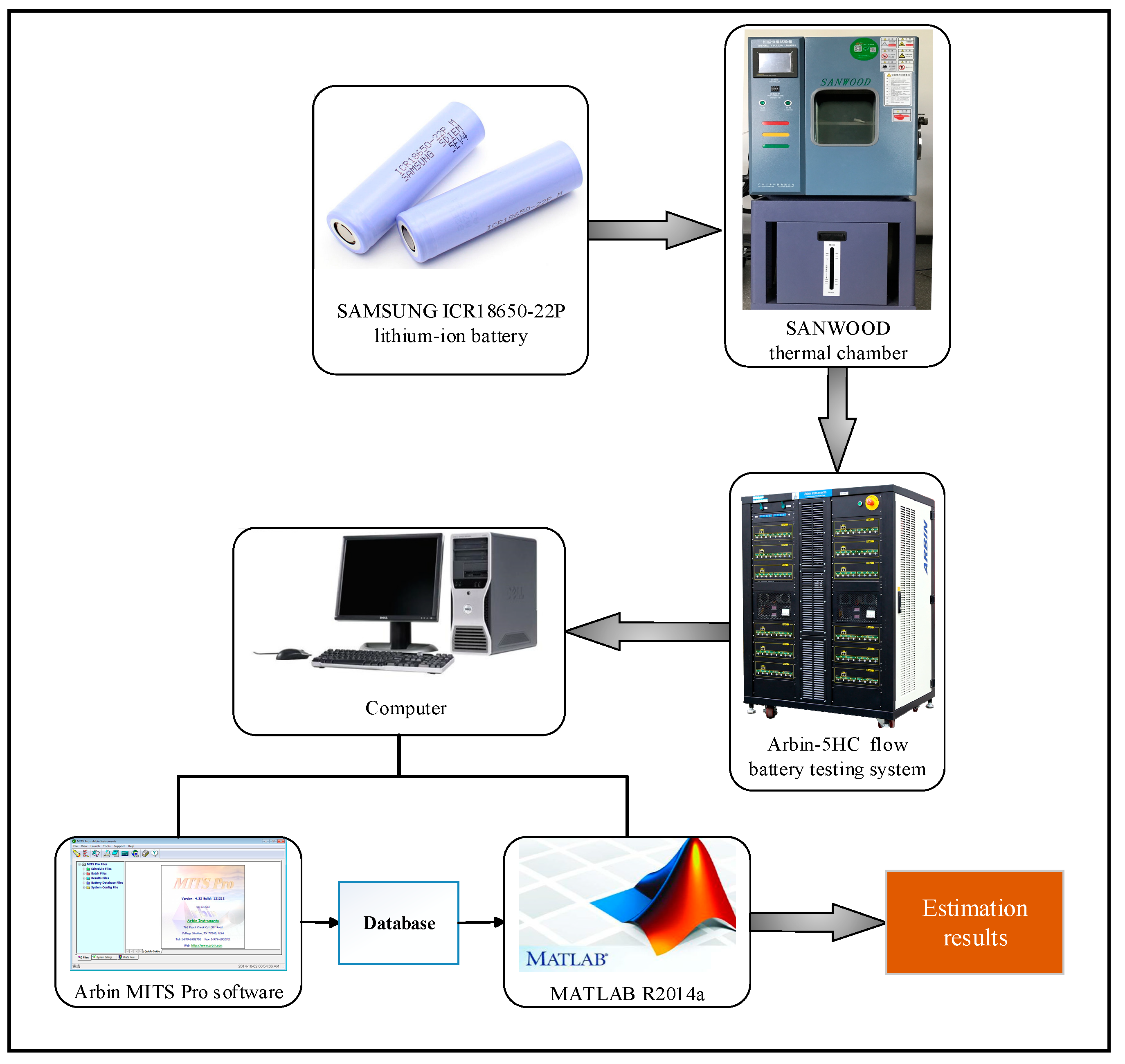
As shown in Figure 4, the experimental platform was established to verify the feasibility and effectiveness of the proposed algorithms. The battery was placed in a thermal chamber that could provide a steady-state temperature to prevent environmental effects. A 5HC Arbin flow battery testing system with eight independent channels was employed to manage the charge/discharge process and collect battery information, such as voltage, current, and resistance. The information was transmitted to a computer and saved using the MITS Pro software.
4.2. Estimation Results with White Gaussian Noises
To verify the performance of the proposed strong tracking H-infinity filter method, the New Europe Driving Cycle (NEDC) test was conducted to simulate the typical operating condition of batteries. The current profile of the NEDC test is shown in Figure 5. The current and voltage can be measured and recorded using the workbench, which can be viewed as exact values. Once the precise current and voltage are determined, the true value of the SOC can be obtained using the Ah counting method. However, in the practical environment, the precise current and voltage could not be obtained because of the precision of the sensors. Therefore, the common white Gaussian noise was added to the measured data to simulate the practical reality. The variances of the zero-mean current and voltage noises were 10−2 and 10−4, respectively.
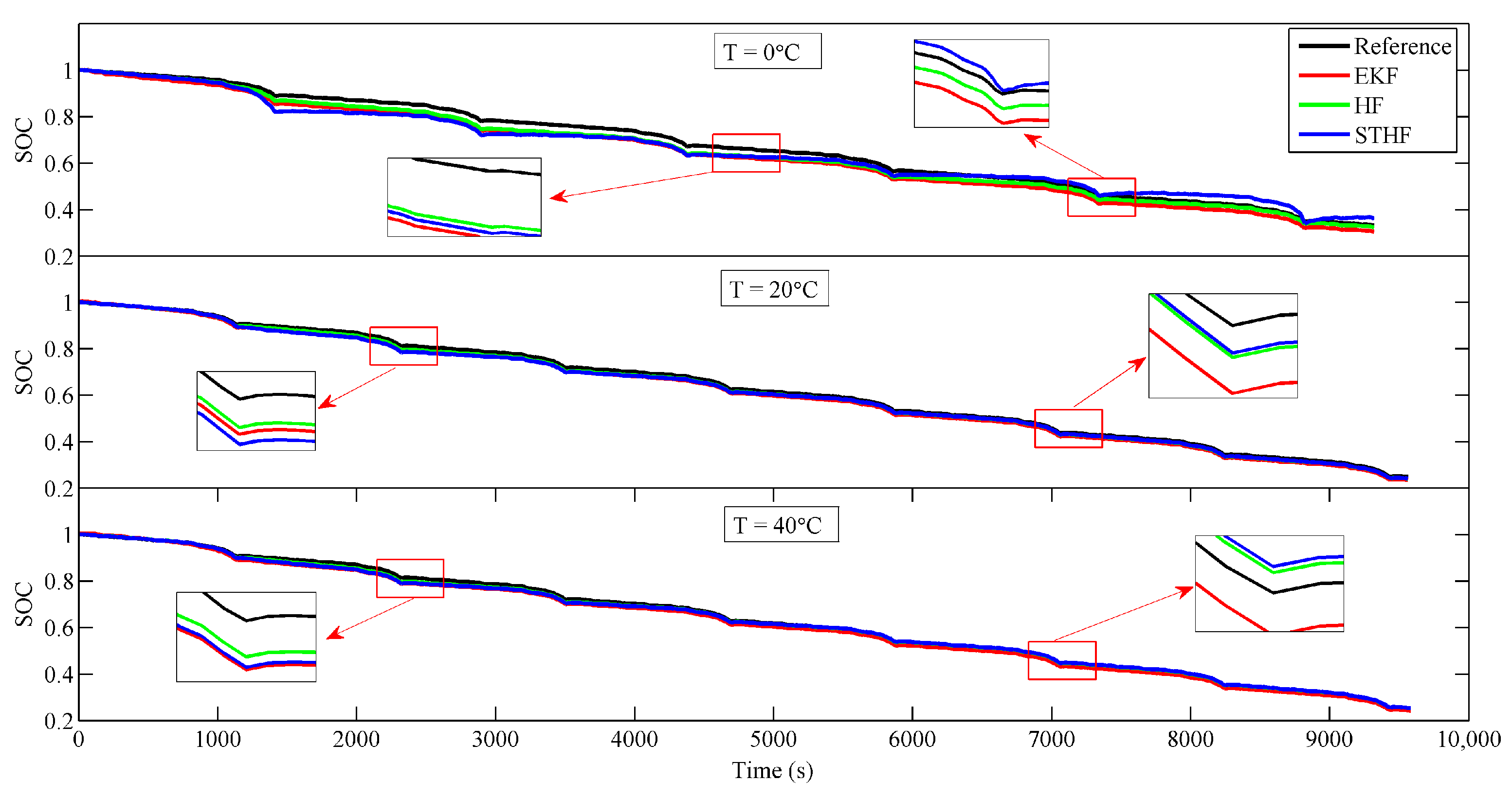
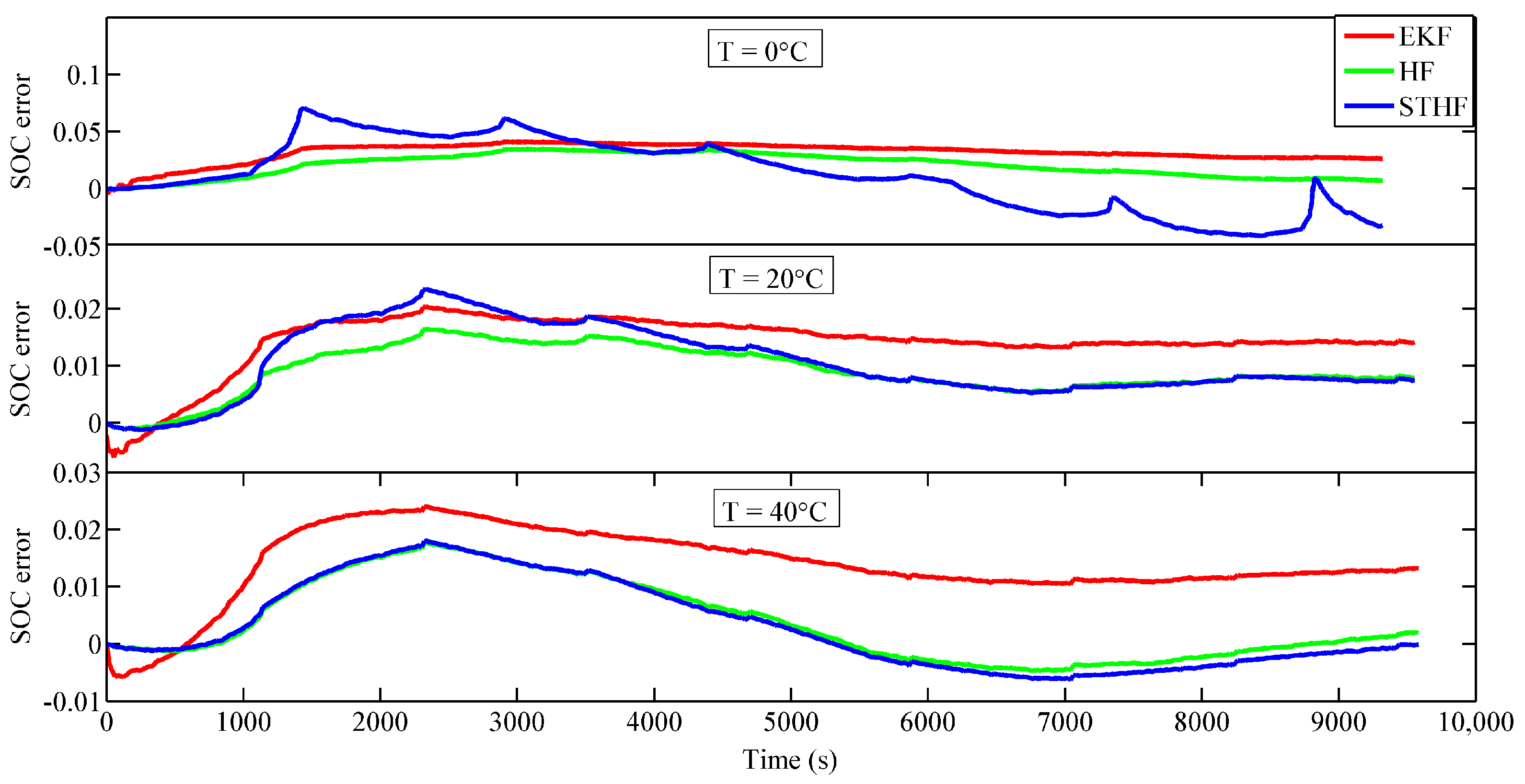
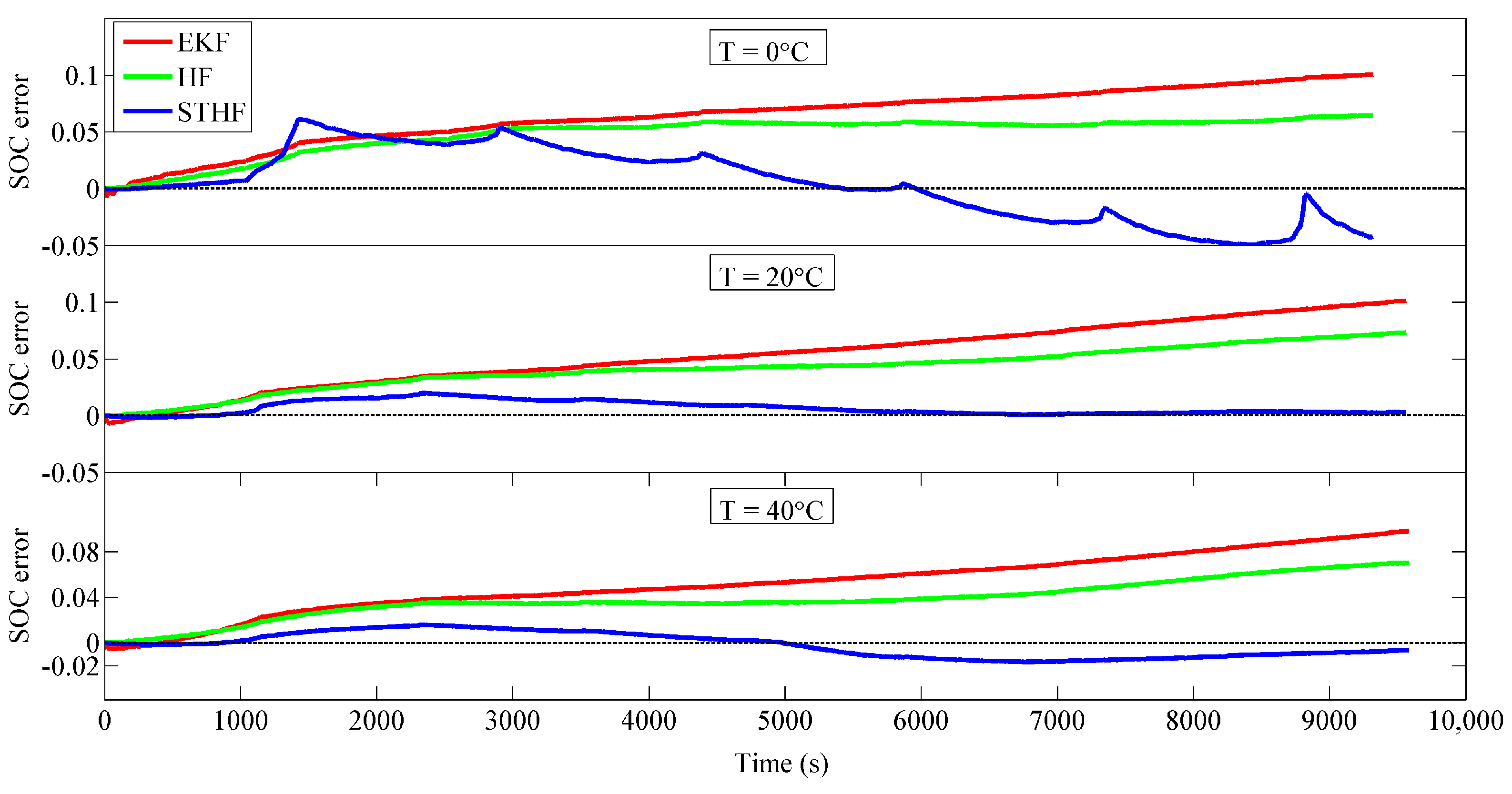
The estimation results obtained using the STHF method at different temperatures are shown in Figure 6, and the estimation error is illustrated in Figure 7. The reference value of the SOC was calculated using the Ah counting method. The estimation results obtained using the HF and EKF are also shown in Figure 6 and Figure 7 for comparison. The estimation procedure employed in the HF method is summarized in Table 3. The EKF method for battery SOC estimation is widely studied, and the process of this algorithm is introduced in Pérez et al., Hu et al., Xiong et al., Chiang et al., and Lee et al. [16,42,43,44,45]; thus, the details are not discussed in the current study. To achieve fairness, the parameters of EKF and STHF are assigned identical values, as listed in Table 5.
The mean absolute error (MAE) and the maximal error of the three methods at 0 °C, 20 °C, and 40 °C are listed in Table 6. The aforementioned results suggest that the estimation error of the STHF method was close to that of the HF method at 20 °C and 40 °C but was more accurate than that of the EKF method. At 0 °C, the estimation results obtained using the STHF method were unstable and were likely to exhibit fluctuation.
4.3. Robustness against Biased Measured Noises
The estimation accuracy obtained for white Gaussian noise by using the STHF method was discussed and compared with those values obtained using other algorithms in Section 4.2. However, the assumed zero-mean noise hardly occurred in the practical reality. Thus, the robustness of the STHF method against biased measurement noise was verified in this section.
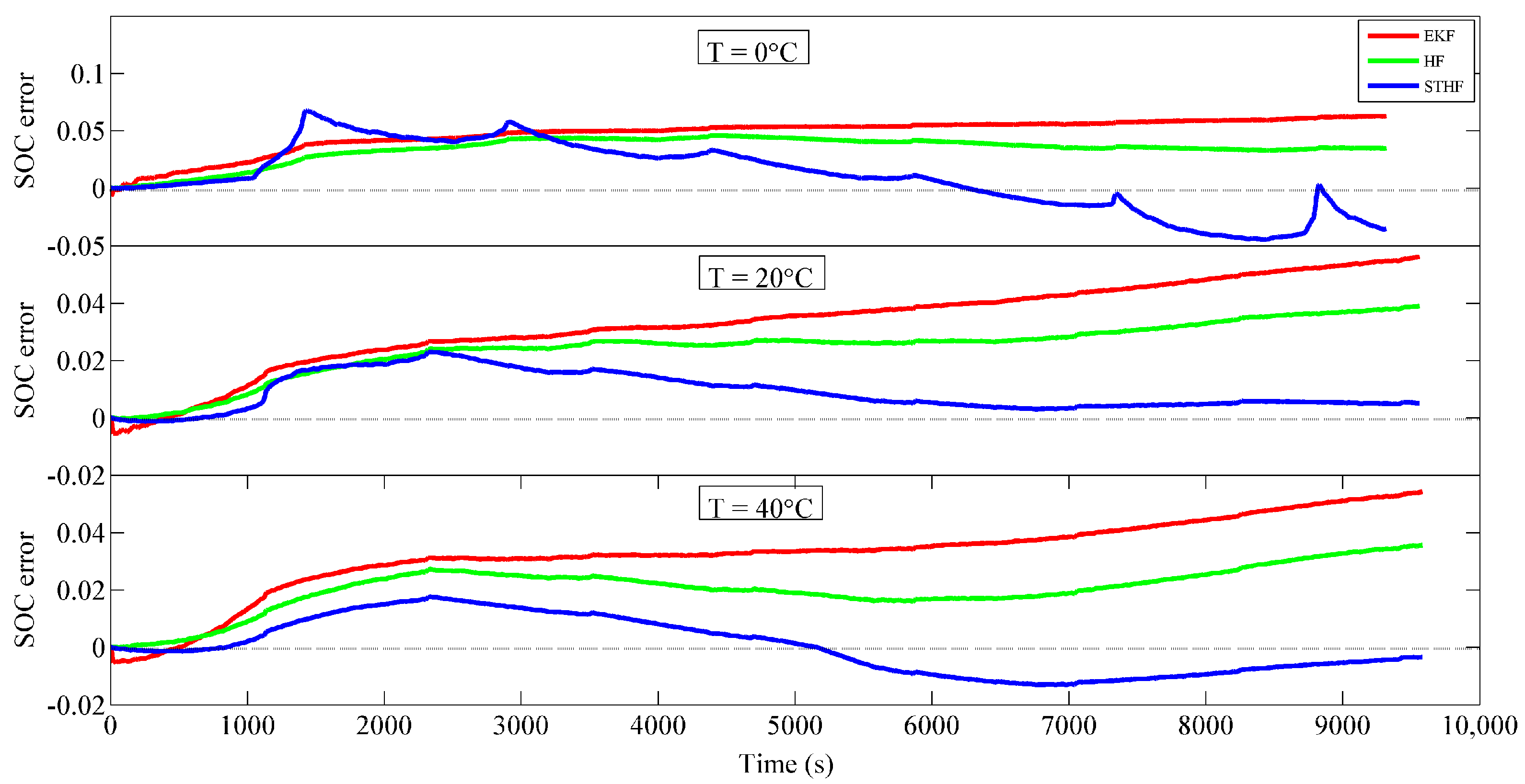
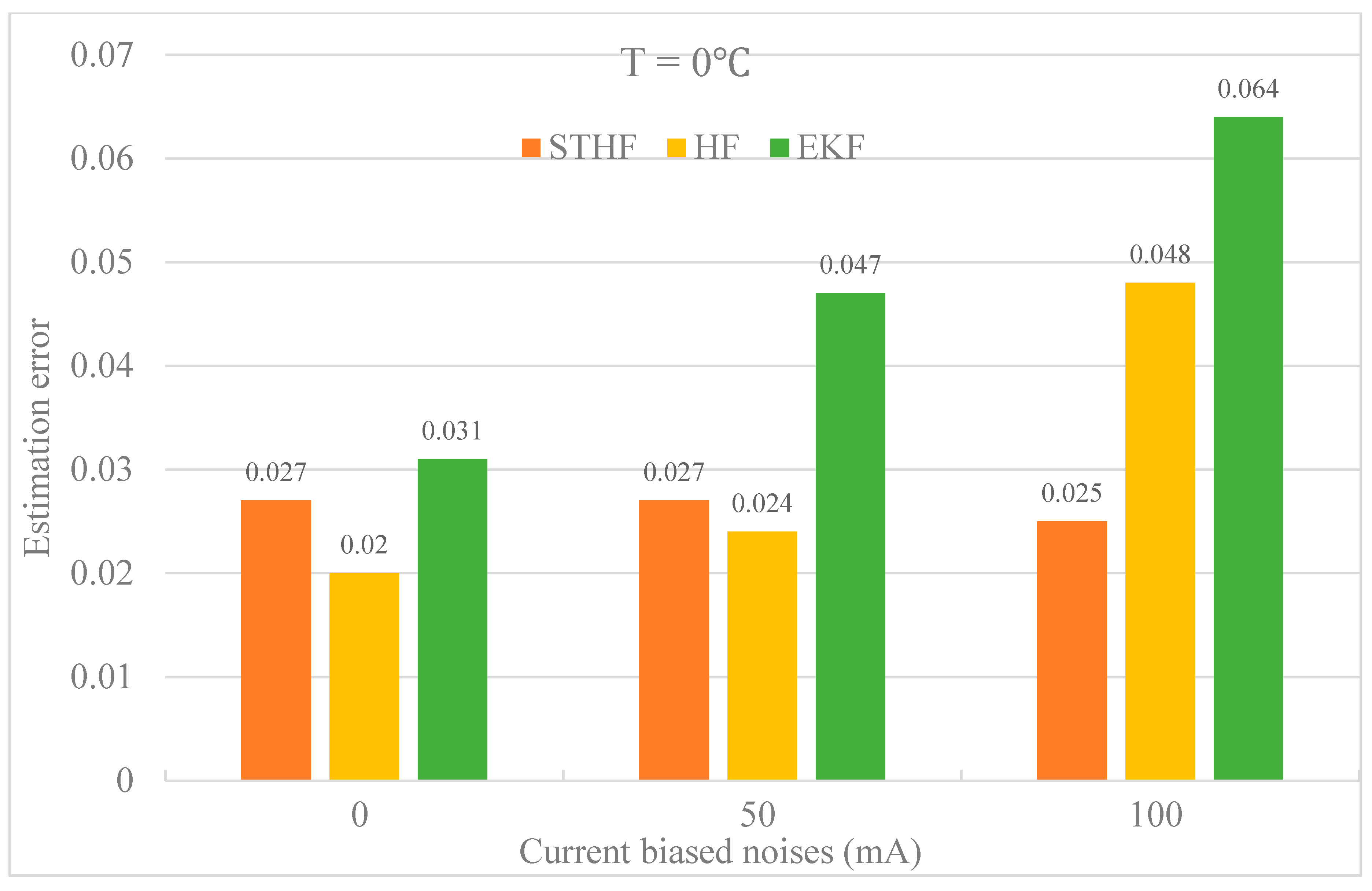
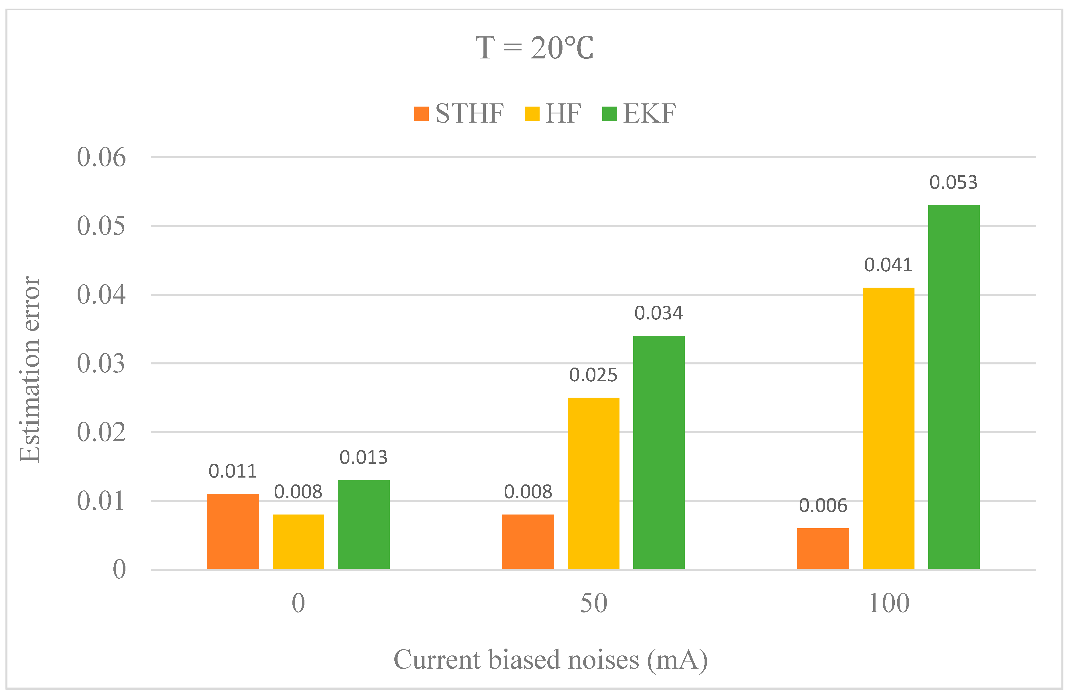
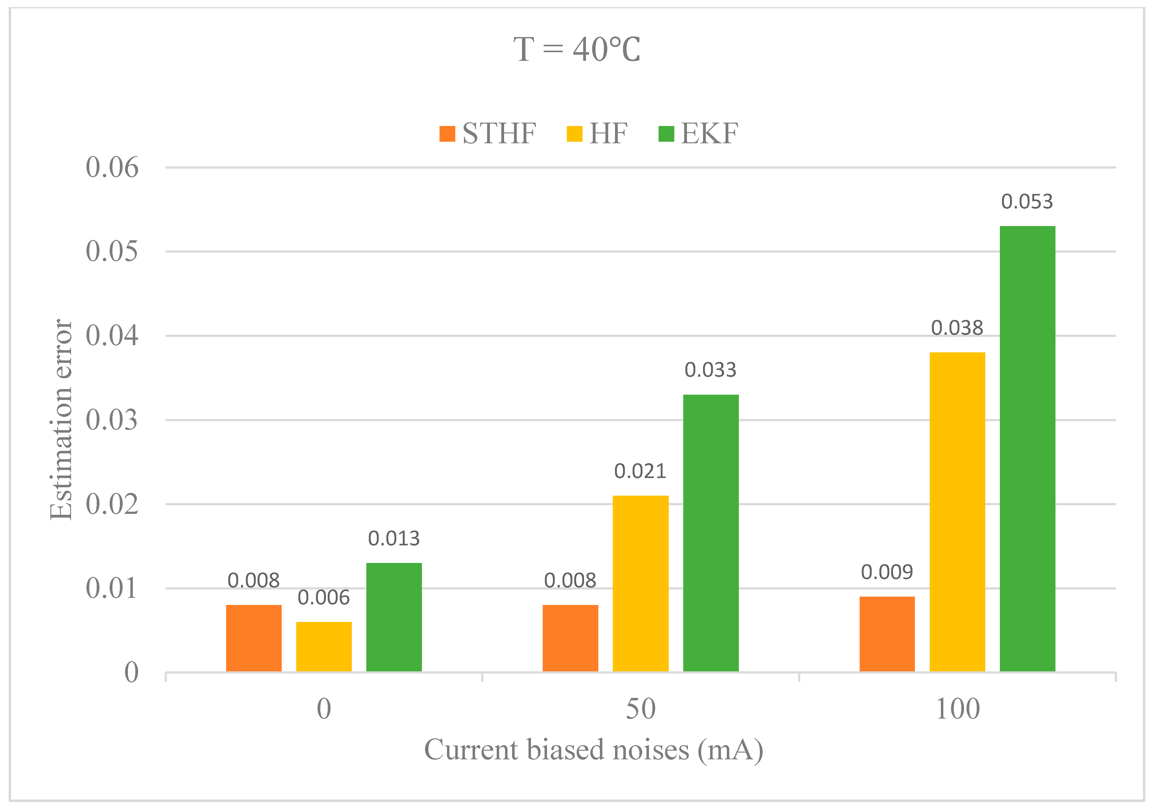
For this purpose, the 0.05 and 0.1 A current-biased noises were added to the data of the NEDC test, and the SOC was estimated using the STHF, HF, and EKF methods. Figure 8 shows the results of estimation with the 0.05 A current-biased noises, obtained using the three methods at different temperatures. Figure 9 shows the corresponding estimation error. Figure 10 and Figure 11 present the estimation results and error with 0.1 A current-biased noises, respectively. The MAEs of the three methods are shown in Figure 12, Figure 13 and Figure 14.
The MAE of the STHF method slightly changed when the current-biased noises were present; however, the MAE of the HF and EKF methods increased rapidly. As shown in Figure 12, Figure 13 and Figure 14, the estimation errors of HF and EKF tended to diverge, but the estimation results of the STHF still converged to the reference value. Thus, compared with the other methods, the STHF approach exhibited a stronger robustness against the biased measured noises, which was more in line with reality.
4.4. Robustness against Initial Error
Another main reason for SOC inaccuracy was the initial error. In many cases, the accuracy of the initial state cannot be predetermined. Thus, the robustness against the initial error is an important criterion for evaluating the performance of the algorithms. In this section, the initial SOC was set to 60% when the true value was 100%. Figure 15 illustrates the estimation results, and Figure 16 shows the estimation errors of the three methods when the initial error was 40%.
To compare the convergence rate, the time when the estimation error converged to less than 10% is marked in Figure 16. The convergence times obtained using the STHF method were 1423, 641, and 461 s at 0 °C, 20 °C, and 40 °C, respectively. The convergence times of the HF and EKF methods were considerably longer than that of the STHF approach.
4.5. Estimation Results of Additional Tests
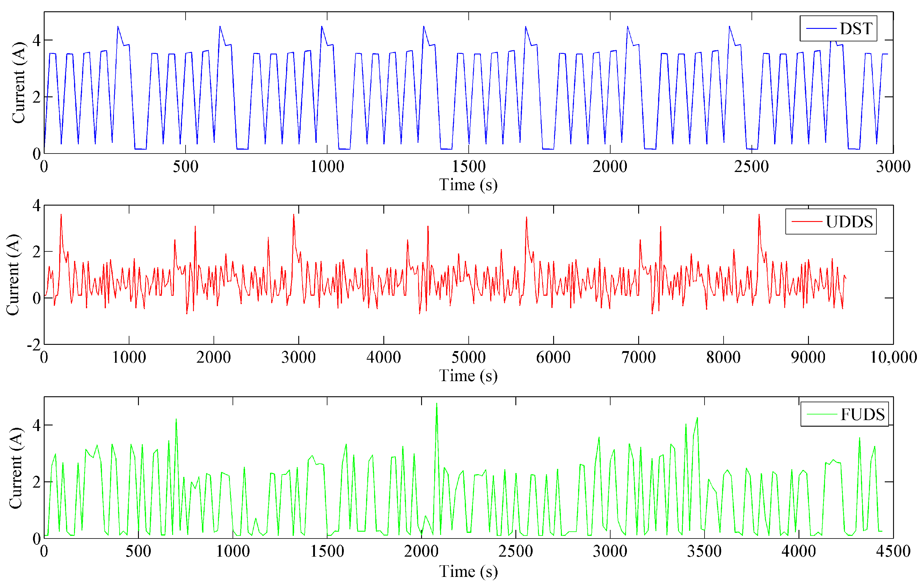
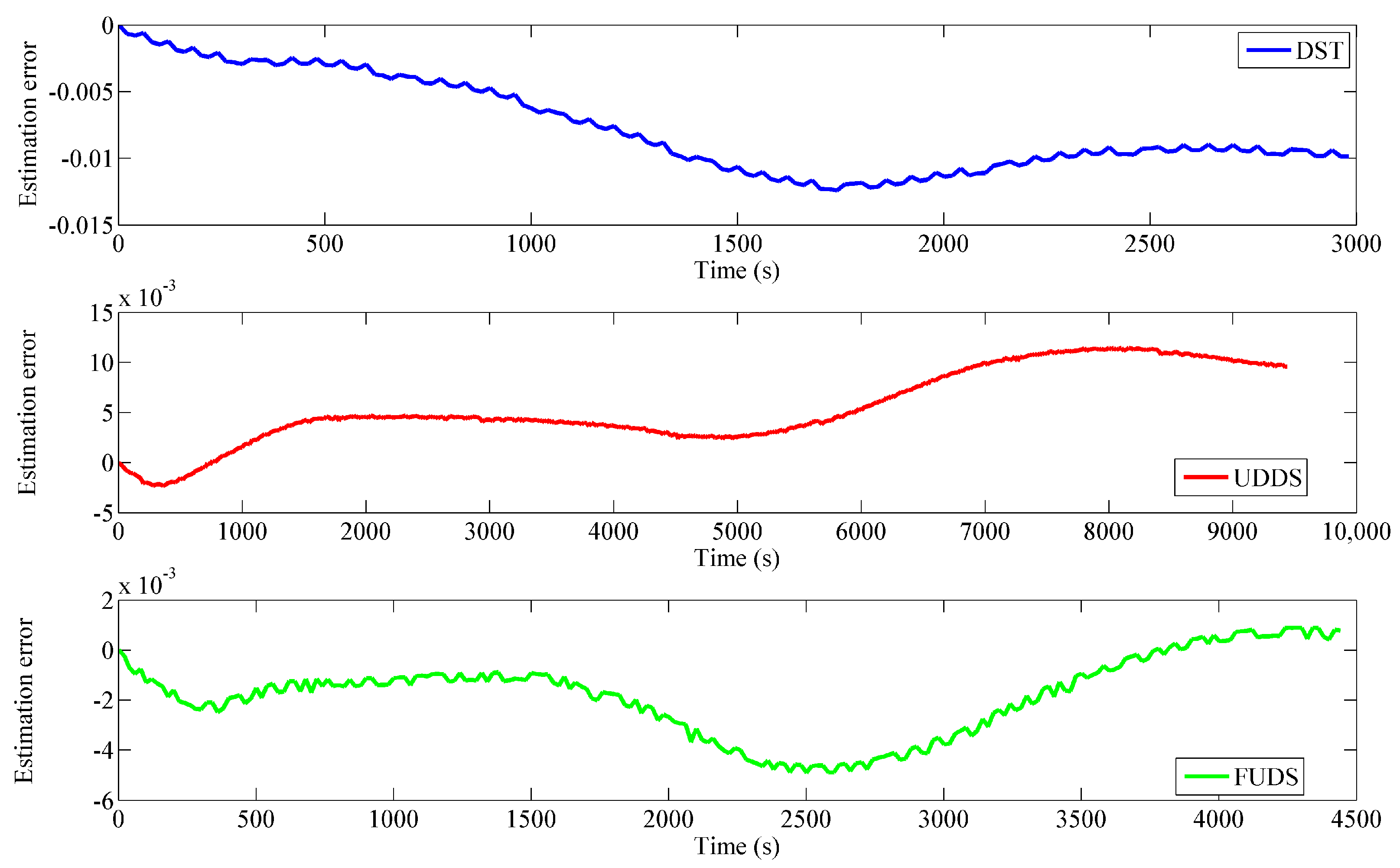
To verify the performance of the STHF method more comprehensively, additional discharge tests were conducted at 25 °C. The Dynamic Stress Test (DST), Urban Dynamometer Driving Schedule (UDDS), and Federal Urban Driving Schedule (FUDS) represent three typical battery test profiles. Figure 17 describes the relationship between discharging current and time. The estimation error of the STHF method at 25 °C under the three test data is shown in Figure 18. The mean absolute error and the maximal error are listed in Table 7. The STHF method clearly shows high estimation accuracy under these battery tests.
4.6. Computational Cost Comparison
Except for the estimation accuracy, the complexity assessment is also important for an algorithm because high computation can affect the hardware cost of BMS and timeliness of estimation results. In this section, the computational time of STHF, HF, and EKF methods are compared under different test profiles. To reduce the error, the algorithms ran three times under each profile and the average results of the three times are shown in Table 8.
Through the data analysis in Table 8, it is obvious that the STHF method required higher computational cost than HF and EKF. But the differences were not enormous, so it can be ignored as the hardware performance improvement in BMS.
5. Conclusions
This work aimed to obtain the accurate SOC of LIBs. To reach this purpose, a novel method was proposed in this paper based on a strong tracking H-infinity filter. First, a commonly used second-order RC equivalent circuit battery model was used, and the parameters of the model were determined by exponential-function fitting. On this basis, the H-infinity filter algorithm was derived based on game theory. The STHF algorithm was then proposed to enhance the robustness of HF. The workbench on which the battery discharging tests were conducted was established. Finally, the battery SOC was estimated using STHF, and the estimation results of HF and EKF were presented for comparison.
The results suggest that the STHF method has higher robustness to measured noise and initial error: (1) if the measured noise is colored noise, estimation using the STHF can obtain high accuracy; (2) when the initial error exists, estimation using STHF can achieve the precise value faster. In summary, owing to its high robustness, the STHF approach is more practical for SOC estimation, particularly under large-noise conditions or in harsh situations.
However, numerous issues can be addressed in future studies. The strong tracking H-infinity filter approach estimates the state of the battery on the basis of the measured voltage; thus, the precision of voltage measurement largely affects the estimation accuracy. In addition, battery experiments are conducted based on a single cell in this study. The effectiveness of the STHF method on the battery module or battery pack of the EV needs to be investigated.
Author Contributions
B.X. and Z.Z. proposed the estimation algorithms and designed the comparative experiments; Z.L. performed the battery tests experiments; B.X. contributed reagents and analysis tools; W.W., W.S., Y.L. and M.W. gave experimental guidance and results analysis. Z.Z. wrote the paper.
Funding
This work is mainly supported by Shenzhen Science and Technology Project (No. JCY20150331151358137) and partly supported by Sunwoda Electronics Co., Ltd. and Tsinghua University.
Conflicts of Interest
The authors declare that there is no conflict of interest.
References
- Tian, Y.; Li, D.; Tian, J.; Xia, B. State of charge estimation of lithium-ion batteries using an optimal adaptive gain nonlinear observer. Electrochim. Acta 2017, 225, 225–234. [Google Scholar] [CrossRef]
- Zhang, Z.-L.; Cheng, X.; Lu, Z.-Y.; Gu, D.-J. SOC Estimation of Lithium-Ion Batteries With AEKF and Wavelet Transform Matrix. IEEE Trans. Power Electron. 2017, 32, 7626–7634. [Google Scholar] [CrossRef]
- Lu, L.; Han, X.; Li, J.; Hua, J.; Ouyang, M. A review on the key issues for lithium-ion battery management in electric vehicles. J. Power Sources 2013, 226, 272–288. [Google Scholar] [CrossRef]
- Yang, N.; Zhang, X.; Li, G. State of charge estimation for pulse discharge of a LiFePO4 battery by a revised Ah counting. Electrochim. Acta 2015, 151, 63–71. [Google Scholar] [CrossRef]
- Xia, B.; Sun, Z.; Zhang, R.; Lao, Z. A Cubature Particle Filter Algorithm to Estimate the State of the Charge of Lithium-Ion Batteries Based on a Second-Order Equivalent Circuit Model. Energies 2017, 10, 457. [Google Scholar] [CrossRef]
- Ng, K.S.; Moo, C.-S.; Chen, Y.-P.; Hsieh, Y.-C. Enhanced coulomb counting method for estimating state-of-charge and state-of-health of lithium-ion batteries. Appl. Energy 2009, 86, 1506–1511. [Google Scholar] [CrossRef]
- Ng, K.S.; Moo, C.S.; Chen, Y.P.; Hsieh, Y.C. State-of-charge estimation for lead-acid batteries based on dynamic open-circuit voltage. In Proceedings of the IEEE International Power and Energy Conference, Johor Bahru, Malaysia, 1–3 December 2008; pp. 972–976. [Google Scholar]
- Zou, Z.; Xu, J.; Mi, C.; Cao, B.; Chen, Z. Evaluation of Model Based State of Charge Estimation Methods for Lithium-Ion Batteries. Energies 2014, 7, 5065–5082. [Google Scholar] [CrossRef] [Green Version]
- Li, Z.; Huang, J.; Liaw, B.Y.; Zhang, J. On state-of-charge determination for lithium-ion batteries. J. Power Sources 2017, 348, 281–301. [Google Scholar] [CrossRef]
- Waag, W.; Fleischer, C.; Sauer, D.U. Critical review of the methods for monitoring of lithium-ion batteries in electric and hybrid vehicles. J. Power Sources 2014, 258, 321–339. [Google Scholar] [CrossRef]
- Huang, S.-C.; Tseng, K.-H.; Liang, J.-W.; Chang, C.-L.; Pecht, M. An Online SOC and SOH Estimation Model for Lithium-Ion Batteries. Energies 2017, 10, 512. [Google Scholar] [CrossRef]
- He, W.; Williard, N.; Chen, C.; Pecht, M. State of charge estimation for Li-ion batteries using neural network modeling and unscented Kalman filter-based error cancellation. Int. J. Electr. PowerEnergy Syst. 2014, 62, 783–791. [Google Scholar] [CrossRef]
- Song, C.; Shao, Y.; Song, S.; Chang, C.; Zhou, F.; Peng, S.; Xiao, F. Energy Management of Parallel-Connected Cells in Electric Vehicles Based on Fuzzy Logic Control. Energies 2017, 10, 404. [Google Scholar] [CrossRef]
- Xing, Y.; He, W.; Pecht, M.; Tsui, K.L. State of charge estimation of lithium-ion batteries using the open-circuit voltage at various ambient temperatures. Appl. Energy 2014, 113, 106–115. [Google Scholar] [CrossRef]
- Lin, C.; Tang, A.; Xing, J. Evaluation of electrochemical models based battery state-of-charge estimation approaches for electric vehicles. Appl. Energy 2017, 207, 394–404. [Google Scholar] [CrossRef]
- Pérez, G.; Garmendia, M.; Reynaud, J.F.; Crego, J.; Viscarret, U. Enhanced closed loop State of Charge estimator for lithium-ion batteries based on Extended Kalman Filter. Appl. Energy 2015, 155, 834–845. [Google Scholar] [CrossRef]
- Xia, B.; Wang, H.; Wang, M.; Sun, W.; Xu, Z.; Lai, Y. A New Method for State of Charge Estimation of Lithium-Ion Battery Based on Strong Tracking Cubature Kalman Filter. Energies 2015, 8, 13458–13472. [Google Scholar] [CrossRef] [Green Version]
- Tian, Y.; Xia, B.; Sun, W.; Xu, Z.; Zheng, W. A modified model based state of charge estimation of power lithium-ion batteries using unscented Kalman filter. J. Power Sources 2014, 270, 619–626. [Google Scholar] [CrossRef]
- Xia, B.; Sun, Z.; Zhang, R.; Cui, D.; Lao, Z.; Wang, W.; Sun, W.; Lai, Y.; Wang, M. A Comparative Study of Three Improved Algorithms Based on Particle Filter Algorithms in SOC Estimation of Lithium Ion Batteries. Energies 2017, 10, 1149. [Google Scholar] [CrossRef]
- Zhong, Q.; Zhong, F.; Cheng, J.; Li, H.; Zhong, S. State of charge estimation of lithium-ion batteries using fractional order sliding mode observer. ISA Trans. 2017, 66, 448–459. [Google Scholar] [CrossRef] [PubMed]
- Xia, B.; Zheng, W.; Zhang, R.; Lao, Z.; Sun, Z. A Novel Observer for Lithium-Ion Battery State of Charge Estimation in Electric Vehicles Based on a Second-Order Equivalent Circuit Model. Energies 2017, 10, 1150. [Google Scholar] [CrossRef]
- Yan, J.; Xu, G.; Xu, Y.; Xie, B. Battery state-of-charge estimation based on H∞ filter for hybrid electric vehicle. In Proceedings of the International Conference on Control, Automation, Robotics and Vision, Hanoi, Vietnam, 17–20 December 2008; pp. 464–469. [Google Scholar]
- Zhang, F.; Liu, G.; Fang, L.; Wang, H. Estimation of Battery State of Charge With H∞ Observer: Applied to a Robot for Inspecting Power Transmission Lines. IEEE Trans. Ind. Electron. 2012, 59, 1086–1095. [Google Scholar] [CrossRef]
- Chen, Y.; Huang, D.; Feng, D.; Wei, K. An H∞ filter based approach for battery SOC estimation with performance analysis. In Proceedings of the IEEE International Conference on Mechatronics and Automation, Beijing, China, 2–5 August 2015; pp. 1613–1618. [Google Scholar]
- Lin, C.; Mu, H.; Xiong, R.; Shen, W. A novel multi-model probability battery state of charge estimation approach for electric vehicles using H-infinity algorithm. Appl. Energy 2016, 166, 76–83. [Google Scholar] [CrossRef]
- Zhang, Y.; Xiong, R.; He, H.; Shen, W. Lithium-Ion Battery Pack State of Charge and State of Energy Estimation Algorithms Using a Hardware-in-the-Loop Validation. IEEE Trans. Power Electron. 2017, 32, 4421–4431. [Google Scholar] [CrossRef]
- Chen, C.; Xiong, R.; Shen, W. A Lithium-Ion Battery-in-the-Loop Approach to Test and Validate Multiscale Dual H Infinity Filters for State-of-Charge and Capacity Estimation. IEEE Trans. Power Electron. 2018, 33, 332–342. [Google Scholar] [CrossRef]
- Alfi, A.; Haddad Zarif, M.; Charkhgard, M. Hybrid state of charge estimation for lithium-ion batteries: Design and implementation. IET Power Electron. 2014, 7, 2758–2764. [Google Scholar] [CrossRef]
- Yu, Q.; Xiong, R.; Lin, C.; Shen, W.; Deng, J. Lithium-Ion Battery Parameters and State-of-Charge Joint Estimation Based on H-Infinity and Unscented Kalman Filters. IEEE Trans. Veh. Technol. 2017, 66, 8693–8701. [Google Scholar] [CrossRef]
- Zhu, Q.; Li, L.; Hu, X.; Xiong, N.; Hu, G.-D. H∞-Based Nonlinear Observer Design for State of Charge Estimation of Lithium-Ion Battery With Polynomial Parameters. IEEE Trans. Veh. Technol. 2017, 66, 10853–10865. [Google Scholar] [CrossRef]
- Liu, C.-Z.; Zhu, Q.; Li, L.; Liu, W.-Q.; Wang, L.-Y.; Xiong, N.; Wang, X.-Y. A State of Charge Estimation Method Based on H∞ Observer for Switched Systems of Lithium-Ion Nickel–Manganese–Cobalt Batteries. IEEE Trans. Ind. Electron. 2017, 64, 8128–8137. [Google Scholar] [CrossRef]
- Wang, C.; He, H.; Zhang, Y.; Mu, H. A comparative study on the applicability of ultracapacitor models for electric vehicles under different temperatures. Appl. Energy 2017, 196, 268–278. [Google Scholar] [CrossRef]
- Samad, N.A.; Wang, B.; Siegel, J.B.; Stefanopoulou, A.G. Parameterization of Battery Electro-Thermal Models Coupled with Finite Element Flow Models for Cooling. J. Dyn. Syst. Meas. Control 2017, 139, 071003. [Google Scholar] [CrossRef]
- Mathew, M.; Kong, Q.H.; McGrory, J.; Fowler, M. Simulation of lithium ion battery replacement in a battery pack for application in electric vehicles. J. Power Sources 2017, 349, 94–104. [Google Scholar] [CrossRef]
- Zhang, X.; Lu, J.; Yuan, S.; Yang, J.; Zhou, X. A novel method for identification of lithium-ion battery equivalent circuit model parameters considering electrochemical properties. J. Power Sources 2017, 345, 21–29. [Google Scholar] [CrossRef]
- Burgos, C.; Sáez, D.; Orchard, M.E.; Cárdenas, R. Fuzzy modelling for the state-of-charge estimation of lead-acid batteries. J. Power Sources 2015, 274, 355–366. [Google Scholar] [CrossRef]
- Shen, X.; Deng, L. Game theory approach to discrete H ∞ filter design. IEEE Trans. Signal Proc. 1997, 45, 1092–1095. [Google Scholar] [CrossRef]
- Dan, S. Optimal State Estimation: Kalman, H∞, and Nonlinear Approaches; Wiley-Interscience: Hoboken, NJ, USA, 2006. [Google Scholar]
- Zhou, D.; Xi, Y.; Zhang, Z. A suboptimal multiple fading extended Kalman Filter. Acta Autom. Sin. 1991, 17, 689–695. [Google Scholar]
- He, X.; Wang, Z.; Wang, X.; Zhou, D.H. Networked Strong Tracking Filtering with Multiple Packet Dropouts: Algorithms and Applications. IEEE Trans. Ind. Electron. 2014, 61, 1454–1463. [Google Scholar] [CrossRef]
- Bai, M.; Zhou, D.H.; Schwarz, H. Adaptive augmented state feedback control for an experimental planar two-link flexible manipulator. IEEE Trans. Robot. Autom. 1998, 14, 940–950. [Google Scholar] [CrossRef]
- Hu, C.; Youn, B.D.; Chung, J. A multiscale framework with extended Kalman filter for lithium-ion battery SOC and capacity estimation. Appl. Energy 2012, 92, 694–704. [Google Scholar] [CrossRef]
- Xiong, R.; Sun, F.; Chen, Z.; He, H. A data-driven multi-scale extended Kalman filtering based parameter and state estimation approach of lithium-ion olymer battery in electric vehicles. Appl. Energy 2014, 113, 463–476. [Google Scholar] [CrossRef]
- Chiang, C.-J.; Yang, J.-L.; Cheng, W.-C. Temperature and state-of-charge estimation in ultracapacitors based on extended Kalman filter. J. Power Sources 2013, 234, 234–243. [Google Scholar] [CrossRef]
- Lee, J.; Nam, O.; Cho, B.H. Li-ion battery SOC estimation method based on the reduced order extended Kalman filtering. J. Power Sources 2007, 174, 9–15. [Google Scholar] [CrossRef]
Figure 1.
Diagram of the second-order resistor–capacitor equivalent circuit model.

Figure 2.
Pulse current discharge experiment procedure.
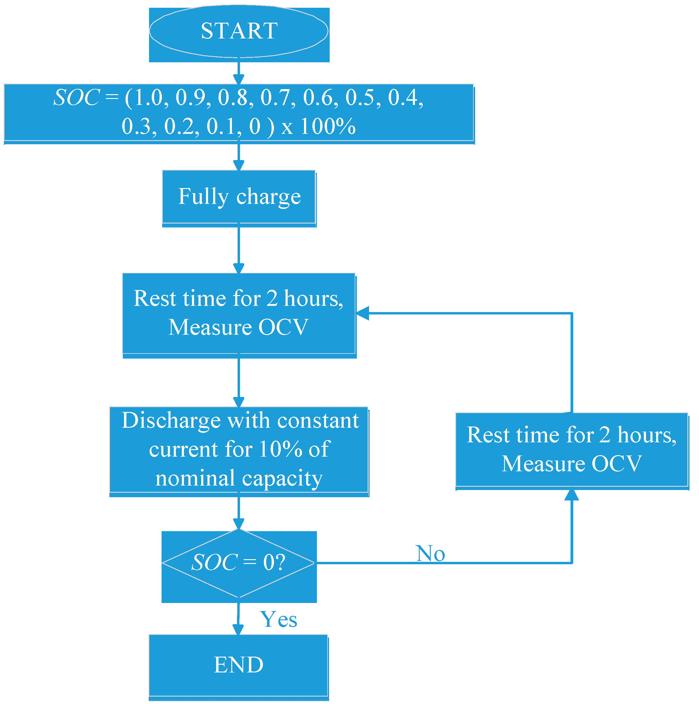
Figure 3.
State of charge (SOC)–open circuit voltage (OCV) nonlinear relationship curve at 0 °C, 20 °C, and 40 °C.
Figure 3.
State of charge (SOC)–open circuit voltage (OCV) nonlinear relationship curve at 0 °C, 20 °C, and 40 °C.
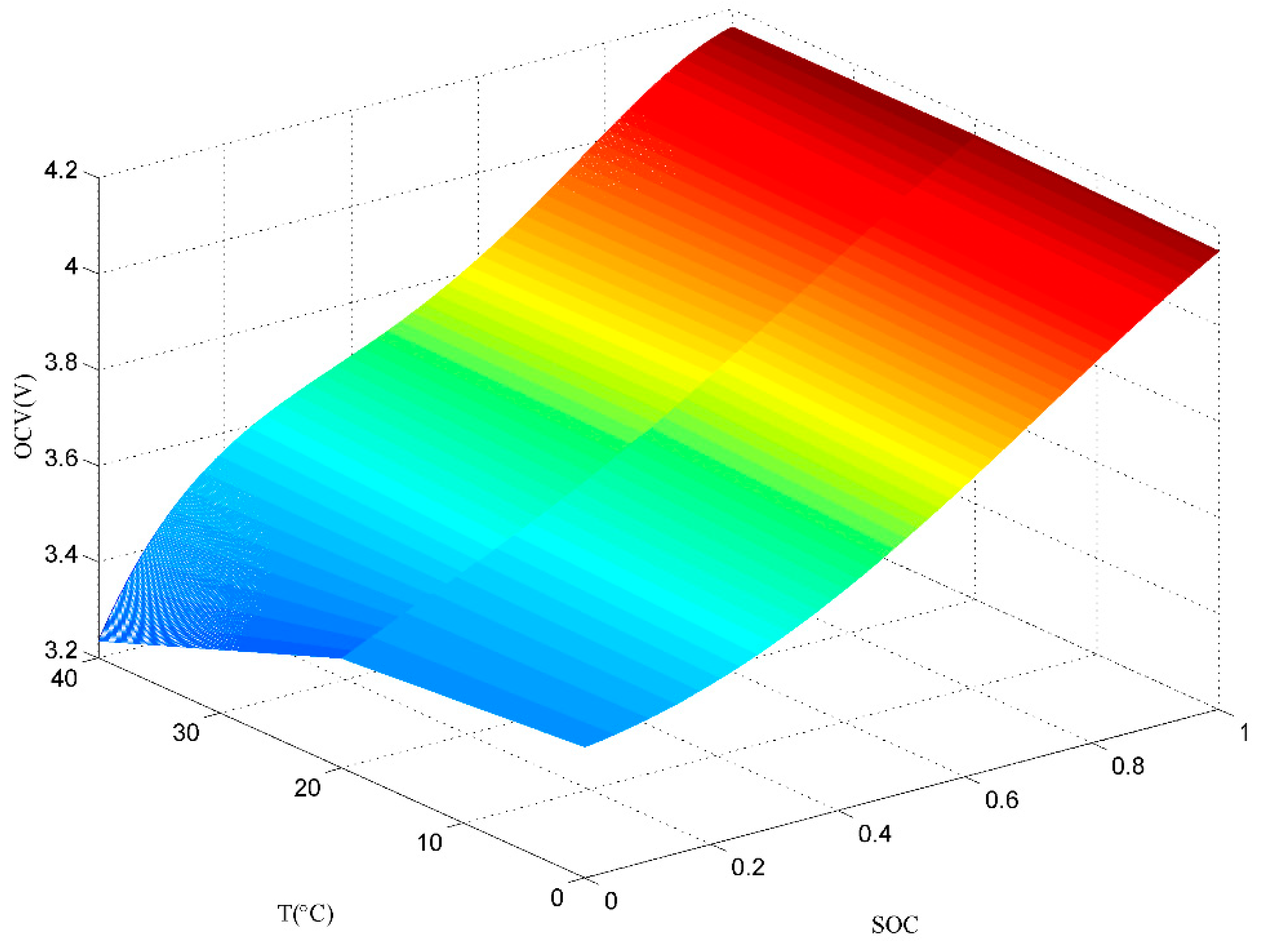
Figure 4.
Diagram of the workbench.

Figure 5.
(a) Discharge current of a complete New Europe Driving Test (NEDC) test; (b) A cycle of the NEDC test.
Figure 5.
(a) Discharge current of a complete New Europe Driving Test (NEDC) test; (b) A cycle of the NEDC test.
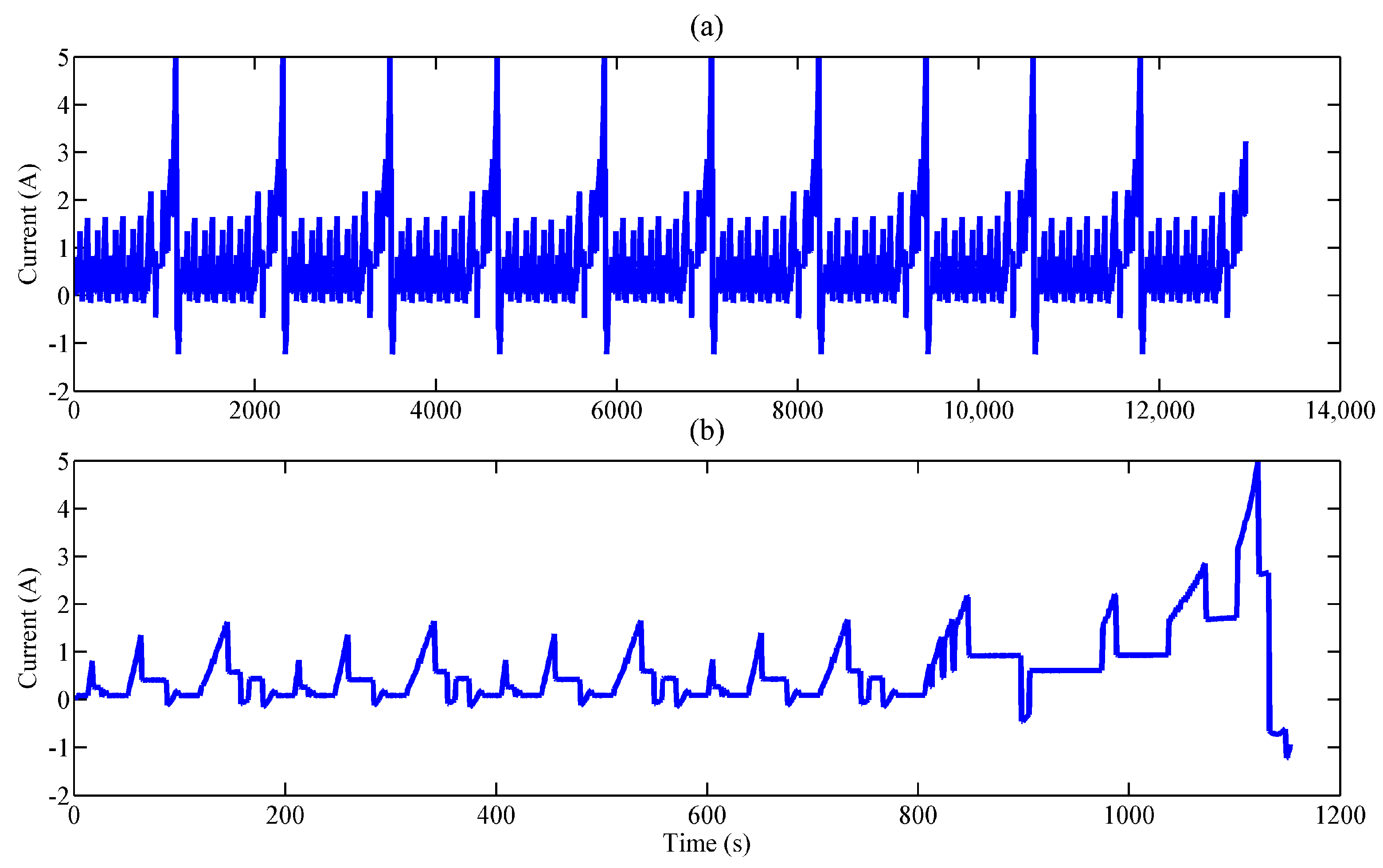
Figure 6.
Estimation results of strong tracking H-infinity filter (STHF), H-infinity filter (HF), and extended Kalman filter (EKF) with white Gaussian noises.
Figure 6.
Estimation results of strong tracking H-infinity filter (STHF), H-infinity filter (HF), and extended Kalman filter (EKF) with white Gaussian noises.

Figure 7.
Estimation errors of STHF, HF, and EKF with white Gaussian noises.

Figure 8.
Estimation results of STHF, HF, and EKF with 0.05 A current-biased noises.
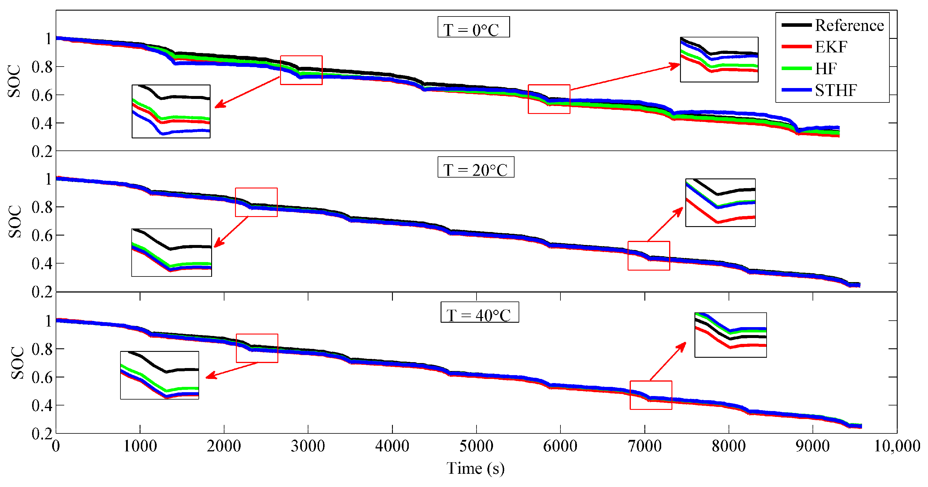
Figure 9.
Estimation errors of STHF, HF and EKF with 0.05 A current-biased noises.

Figure 10.
Estimation results of STHF, HF, and EKF with 0.1 A current-biased noises.
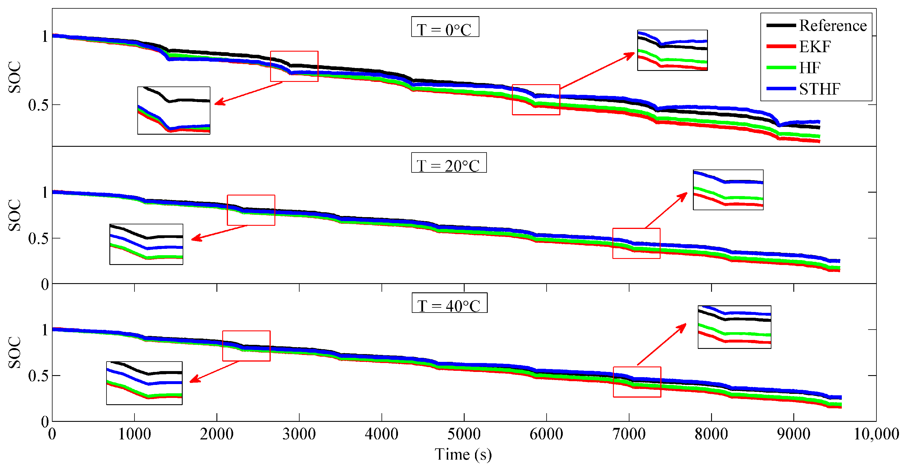
Figure 11.
Estimation errors of STHF, HF, and EKF with 0.1 A current-biased noises.

Figure 12.
Mean absolute errors of STHF, HF, and EKF at 0 °C.

Figure 13.
Mean absolute errors of STHF, HF, and EKF at 20 °C.

Figure 14.
Mean absolute errors of STHF, HF, and EKF at 40 °C.

Figure 15.
Estimation results of STHF, HF, and EKF with an initial error.
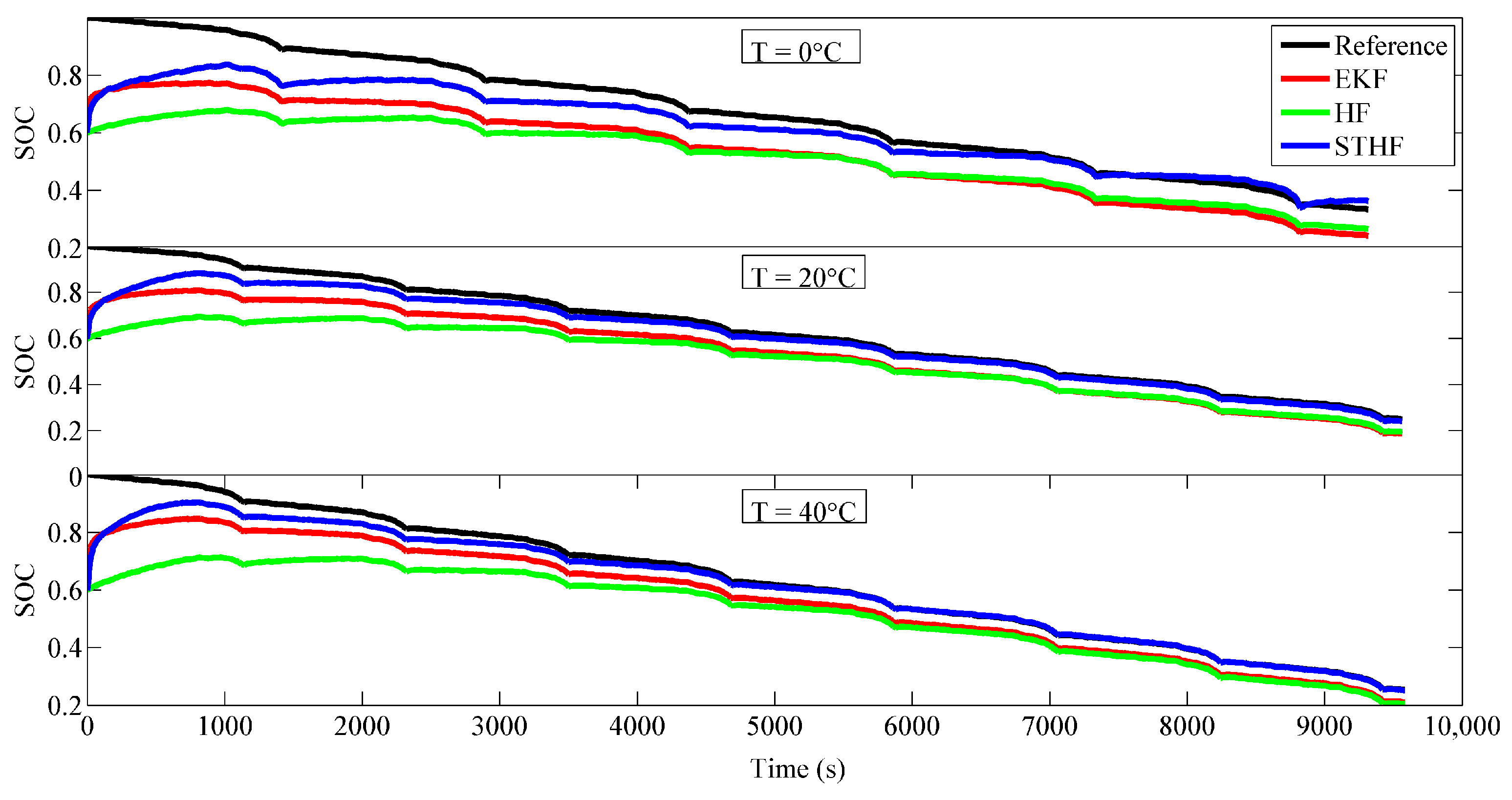
Figure 16.
Estimation errors of STHF, HF, and EKF with an initial error.
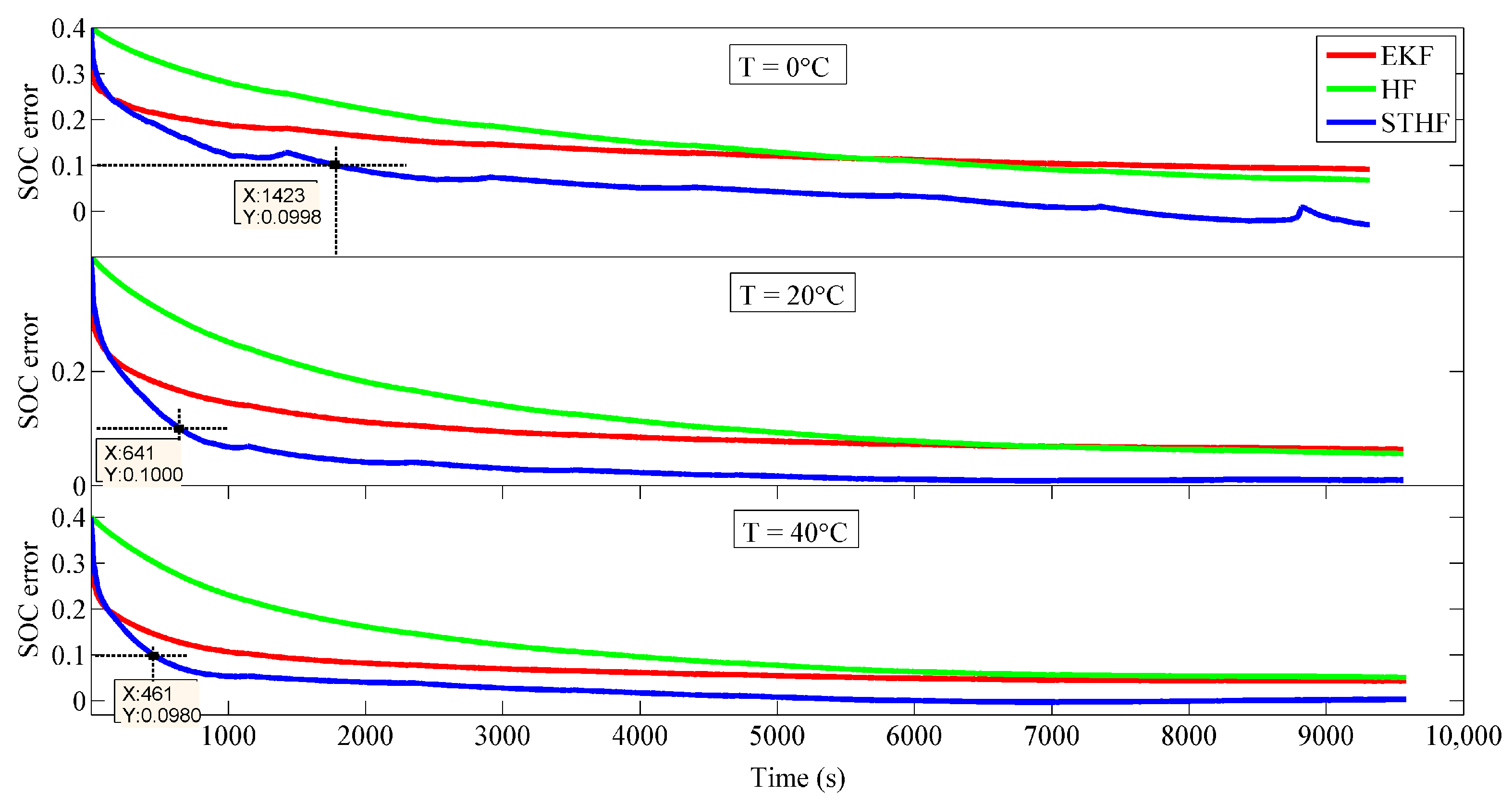
Figure 17.
Discharge current of Dynamic Stress Test (DST), Urban Dynamometer Driving Schedule (UDDS), and Federal Urban Driving Schedule (FUDS) tests.
Figure 17.
Discharge current of Dynamic Stress Test (DST), Urban Dynamometer Driving Schedule (UDDS), and Federal Urban Driving Schedule (FUDS) tests.

Figure 18.
Estimation errors of DST, UDDS, and FUDS tests.


Table 1.
Basic specifications of Samsung ICR18650-22P lithium-ion battery.
| Typical capacity | 2150 mAh |
| Nominal voltage | 3.6 V |
| Charging cut-off voltage | 4.2 ± 0.05 V |
| Discharge cut-off voltage | 2.75 V |
| Max. charge current | 2150 mA |
| Max. discharge current | 10 A |
Table 2.
Identification of battery model parameters at different temperatures.
| T (°C) | R0 (Ω) | R1 (Ω) | R2 (Ω) | C1 (F) | C2 (F) |
|---|---|---|---|---|---|
| 0 | 0.0763 | 0.0147 | 0.0060 | 4508.0 | 12,150 |
| 20 | 0.0395 | 0.0107 | 0.0031 | 4721.2 | 17,288 |
| 40 | 0.0292 | 0.0064 | 0.0013 | 3468.2 | 26,659 |
Table 3.
H-infinity (HF) filter algorithm for state of charge (SOC) estimation.
| Input | Current uk, terminal voltage yk at each time, initial SOC x0 L = [1 0 0] Weighting matrices: Sk, P0, Wk, Vk k = 0 |
| Estimation process | Step 1: Determine Step 2: Linearization of Ck Step 3: Find gain matrix Kk Step 4: Calculate estimation of yk Step 5: State estimation at time k + 1 Step 6: Update covariance matrix Step 7: Output SOC estimation at time k + 1 Step 8: Update time k = k + 1 |
| Output |
Table 4.
Strong tracking H-infinity filter (STHF) algorithm for SOC estimation.
| Input | Current uk, terminal voltage yk at each time, initial SOC x0 L = [1 0 0] Current noise covariance Qk and voltage noise covariance Rk Weighting matrices: Sk, P0, Wk, Vk k = 0 |
| Estimation process | Step 1: Determination of Step 2: Linearization of Ck Step 3: Prior estimation Step 4: Calculation of the suboptimal fading factor λ by Equations (25)–(30) Step 5: Updating of the estimation error covariance matrix Pk by STF Step 6: Finding the gain matrix Kk Step 7: Posteriori estimation Step 6: Update of the estimation error covariance matrix by HF Step 7: Output of SOC estimation at time k + 1 Step 8: Evaluation of estimation timesIf no sampling data are given, estimation is ended; else, go to Step 1. |
| Output |
Table 5.
Strong tracking H-infinity filter (STHF) and extended Kalman filter (EKF) parameters.
| Parameters | Values |
|---|---|
| P0 | [0.001, 0, 0; 0, 0.001, 0; 0, 0, 0.001] |
| Q | [0.001, 0, 0; 0, 0.001, 0; 0, 0, 0.001] |
| R | 0.001 |
Table 6.
Mean absolute errors (MAEs) and maximal errors of STHF, HF and EKF.
| Temperature | 0 °C | 20 °C | 40 °C | ||||||
|---|---|---|---|---|---|---|---|---|---|
| Method | STHF | HF | EKF | STHF | HF | EKF | STHF | HF | EKF |
| MAE | 0.027 | 0.02 | 0.031 | 0.011 | 0.008 | 0.013 | 0.008 | 0.006 | 0.013 |
| Maximal error | 0.072 | 0.034 | 0.040 | 0.026 | 0.015 | 0.020 | 0.024 | 0.019 | 0.024 |
Table 7.
MAEs and maximal errors of Dynamic Stress Test (DST), Urban Dynamometer Driving Schedule (UDDS), and Federal Urban Driving Schedule (FUDS) tests.
Table 7.
MAEs and maximal errors of Dynamic Stress Test (DST), Urban Dynamometer Driving Schedule (UDDS), and Federal Urban Driving Schedule (FUDS) tests.
| Test | DST | UDDS | FUDS |
|---|---|---|---|
| MAE | 0.008 | 0.006 | 0.002 |
| Maximal error | 0.012 | 0.012 | 0.005 |
Table 8.
The running time of STHF, HF, and EKF under different test profiles.
| Test | NEDC | DST | UDDS | FUDS |
|---|---|---|---|---|
| STHF | 0.556 | 0.175 | 0.500 | 0.249 |
| HF | 0.523 | 0.158 | 0.428 | 0.226 |
| EKF | 0.481 | 0.145 | 0.383 | 0.207 |
© 2018 by the authors. Licensee MDPI, Basel, Switzerland. This article is an open access article distributed under the terms and conditions of the Creative Commons Attribution (CC BY) license (http://creativecommons.org/licenses/by/4.0/).
Share and Cite
MDPI and ACS Style
Xia, B.; Zhang, Z.; Lao, Z.; Wang, W.; Sun, W.; Lai, Y.; Wang, M. Strong Tracking of a H-Infinity Filter in Lithium-Ion Battery State of Charge Estimation. Energies 2018, 11, 1481. https://doi.org/10.3390/en11061481
AMA Style
Xia B, Zhang Z, Lao Z, Wang W, Sun W, Lai Y, Wang M. Strong Tracking of a H-Infinity Filter in Lithium-Ion Battery State of Charge Estimation. Energies. 2018; 11(6):1481. https://doi.org/10.3390/en11061481
Chicago/Turabian StyleXia, Bizhong, Zheng Zhang, Zizhou Lao, Wei Wang, Wei Sun, Yongzhi Lai, and Mingwang Wang. 2018. "Strong Tracking of a H-Infinity Filter in Lithium-Ion Battery State of Charge Estimation" Energies 11, no. 6: 1481. https://doi.org/10.3390/en11061481
Note that from the first issue of 2016, this journal uses article numbers instead of page numbers. See further details here.