A Dynamic Model for Indoor Temperature Prediction in Buildings


Control Engineering, University of Oulu, P.O. Box 4300, FI-90014 Oulu, Finland
*
Author to whom correspondence should be addressed.
Energies 2018, 11(6), 1477; https://doi.org/10.3390/en11061477
Submission received: 26 April 2018
/
Revised: 1 June 2018
/
Accepted: 5 June 2018
/
Published: 6 June 2018
Abstract
:A novel dynamic model for the temperature inside buildings is presented, aiming to improve energy efficiency by providing predictive information on the heat demand. To analyse the performance and generalizability of the modelling approach, real measurement data was gathered from five different types of buildings. Easily available data from various sources was utilized. The chosen model structure leads to a minimal number of input variables and free parameters. Simulations with real data from five buildings, and applying the identical model structure showed that the average modelling error during the 28-h prediction horizon was constantly below 5%. The results thus demonstrate that the model structure can be standardized and easily applied to predict the indoor temperatures of large buildings. This would finally enable demand side management and the predictive optimization of the heat demand at city level.
1. Introduction
Buildings still use 20–40% of the world’s total energy consumption and Heating, Ventilation and Air Conditioning (HVAC) account almost half of this energy [1]. At the same time, the heating energy is predominantly based on fossil fuels [2]. Considering this, it is the most important to implement new energy efficiency measures for the building sector. In this article, an identification and validation of a novel dynamic model for predicting the indoor temperatures in large buildings is presented. This modelling approach is argued to provide a key tool for demand side management to enable the predictive optimization of the heat demand at district and city level.
As the requirements for energy efficiency are becoming stricter, it is no longer sufficient to consider buildings as isolated elements in energy systems [3]. They have to be considered as active players having storage capabilities and even their own energy production. Therefore, buildings have to be taken into consideration when developing new control and optimization schemes for district heating systems. A concept for optimizing the heat demand in district heating systems has been proposed by the authors in [4] and preliminary results have shown that significant energy savings and peak load cuts can be achieved [4,5]. The concept approaches the subject by predicting the heat consumption and then optimizing the heat production utilizing demand side management. In this context, the thermal mass of buildings plays a major role for controls towards lower energy usage [6,7] and can offer advantage over centralized storage solutions [8]. However, its use is a challenge due to the slow dynamics of heat storage resulting in time delays [9]. Systems with large delays are generally harder to control and require model-based control. At the same time, maintaining the indoor temperature at an acceptable level is important as the control actions should ensure the quality of the living conditions for the residents. Therefore, a mathematical model for the indoor temperature of a building is critical for predicting the energy demand and for enabling control and optimization strategies aiming at higher energy efficiency [10]. Such a model has to be easily reproducible for multiple buildings to achieve wide impact with energy optimization actions. This sets requirements for the simplicity and ease of parametrization of the model. The straightforward implementation in real applications should also be kept in mind. In modern automation, the cost of implementation work plays a key role while the cost of the hardware is decreasing.
Zhao and Magoulès [11], Kramer et al. [12] and Foucquier et al. [13] have all presented extensive reviews of the building modelling literature. This article addresses especially the modelling and prediction of the indoor temperature in buildings. These models are typically based either on physical principles or they are data driven or a combination of both. Models based on physical principles can vary largely from extremely complex to more simplified structures with respect to the number of parameters and variables [14,15,16,17] but they usually need detailed information on the building characteristics and are in general too computationally heavy to be effectively used for control purposes. On the other hand, data driven models [18,19,20,21,22,23,24,25,26,27,28] are based solely on measurements and are typically identified without information on the physical nature of the building properties. Hybrid or grey box models are a combination of data driven and physical modelling approaches [29,30,31,32,33,34,35]. This model type needs sufficient amount of measurement data for parameter identification and some information about the properties of the building. Generally, the methodology adopts a simplified physical model structure and then its parameters are estimated using measured data [36,37].
For the data driven and hybrid models the data acquisition for the identification of the model and for the estimation of the model parameters is an important issue. If physical parameters are used in the model, they could be calculated using information on building characteristics, but this information is not always easily available. One widely used method for obtaining data for parameter estimation is to apply a physical model for the building to generate an artificial data set [38,39,40,41,42,43,44]. This method was also recently used in [45] where a calibrated EnergyPlus model was utilized to train a simplified model. This kind of data collection would be very time consuming and impractical in case of hundreds or thousands of buildings. Other ways to get a representative data sets for the model identification include the use of data with minimum and maximum historical records [21] or collecting data by performing step response tests [46]. Also, many of the reported studies have acquired data from a particular test building for the model identification [47,48,49,50,51,52]. All these ways can be used to collect data although it can be laborious and time consuming. Also the representativeness of the data and the resulting performance of the model in real buildings at normal operating conditions may remain questionable. This is especially the issue when using physical models to generate the data [53].
For wide use of any indoor temperature model, it should be applicable to different types of buildings with minimum extra implementation work. However, almost all of the reported research discussed above focus on a single building for the development and validation of the model. Furthermore, many of the models presented in previous studies needed detailed information about the building properties and large amount of representative measurements together with many parameters. All of this would increase the complexity and the implementation work of the models thus limiting their application to different buildings in real environments. If the models are only tested in one building, it is very much possible that they cannot be transferred directly to another building. It is not certain if the order of the linear model or the number of hidden layers of neurons of the ANN model can be the same in different buildings, if only one building is used for the model development. Then it comes to the amount of work needed to transfer these models into the different buildings. If the model is to be used only to control an individual building, the implementation time will not necessarily be an issue. However, as the intention of the authors is to perform the optimization of the heating demand at district and city level, the short implementation time for the model is crucial. Days of modelling work on one building is not acceptable if there are hundreds or thousands of buildings that need to be modelled.
To overcome the modelling issues presented above, a new dynamic modelling approach to predict the indoor temperature is proposed. To ensure the model generalizability to the whole building stock together with the reasonable prediction accuracy, the main supporting ideas are:
- To combine easily available, existing real measurements, building information and tabular values while minimizing the number of model parameters and inputs,
- To apply the modelling approach for multiple buildings to validate the generalizability.
Motivation for the proposed modelling approach comes from the fact that it has to be easily implemented in a wide range of energy management systems to enable the city level optimization of the heat demand. In this context, fewer amount of parameters, easily available measurements and generalizable model structure are assumed to make the parameter identification of the model easy in comparison to present modelling methods. The above mentioned model properties would allow the wide application of the model as it is intended to be adaptable to multiple buildings [4].
In the next section, the building information and measurement data is described. The proposed modelling approach and the performance analysis for the model are explained in Section 3. The model identification and validation results are presented in Section 4 and the application of the model in the optimization of the heat demand is discussed in Section 5. Finally, the results are discussed in Section 6 and Section 7 contains our conclusions.
2. Building Characteristics and Measurement Data
2.1. Buildings
Five buildings in Finland were employed as the sites for data collection. Buildings A, B and C are located in the city of Oulu, whereas buildings D and E, are located in the city of Jyväskylä. The characteristics of these buildings are presented in Table 1.
The largest construction, building A, is a school building and it is occupied in weekdays during daytime. Heating and ventilation, including the radiator and floor heating systems, are also scheduled according to the occupancy. Building B is an apartment building. This three story building accommodates residents in two upper floors and offices and services on the first floor. The space heating is supplied by radiators. Building C is a municipal hall, a two story building with thermally heavy structure and low occupancy, namely around eight occupants occasionally. The HVAC system is scheduled according to office hours. Building D is a seven story apartment building from the early 1970s. Finally, building E is a four story apartment building built in 2011.
For all the buildings, the heat is provided through a district heating network. The control systems in studied buildings control the heating based on outdoor temperature. This means that the temperature or the flow of the supply water to the heating circuit is controlled according to outdoor temperature. Those are linearly proportional meaning that the temperature of the supply water rises as the outdoor temperature drops.
2.2. Measurements
Altogether 144 h of data measured from five buildings and consisting of heating power together with outdoor and indoor temperatures was used for the model identification and validation. As large buildings typically have time constants of more than 100 h [54], sampling time for all the measurements was one hour. The measurement periods, the number of different locations for indoor temperature sensors and the range of power and outdoor and indoor temperature measurements are presented in Table 2. Locations for indoor temperature sensors were in different parts of the buildings and there was one indoor temperature sensor in each location.
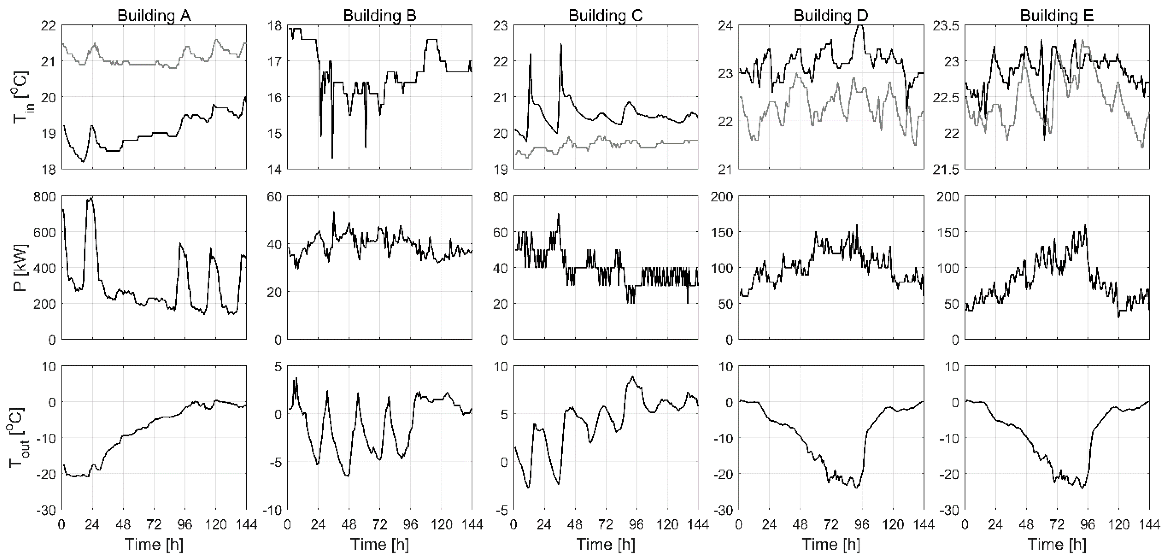
Heating power and outdoor temperature data were provided by district heating companies except for building B where heating power values were calculated from on-site measurements. Also the outdoor temperatures were recorded on-site in building B. During the measurement periods, all the considered buildings were at normal use including the functioning of their control systems. The recorded heating power measurement included the space heating and the usage of hot water. The measurement data is presented in Figure 1, where two indoor temperature measurement locations have been included, except for building B where only one was available.
3. Modelling and Analysis Methods
3.1. General Structure of the Model
The presented model is based on Newton’s cooling law, stating that the rate of heat loss of an object is proportional to the temperature difference between the object and its surroundings. Then, the rate of heat transfer can be formulated as:
where Q is the thermal energy (J), h is the heat transfer coefficient (W/(m2·K)), A is the surface area through which the heat is being transferred (m2), T is the temperature of the object (K) and Tenv is the temperature of the surrounding environment (K).
To make Equation (1) more suitable for the modelling of the indoor temperature, the heat capacity C (J/K) can be expressed as C = dQ/dT, and by differentiating the equation with regard to time gives dQ/dt = C(dT/dt), which can be inserted into Equation (1) to get temperature change instead of energy change. Furthermore, now the temperature of the object is the indoor temperature of the building and the temperature of the surroundings is the outdoor temperature. For simplification, it is assumed that the interior and the building envelope are at the same temperature. Therefore, the entire body of the building can be considered as a lumped capacitance reservoir of heat. Then, applying all this to Equation (1) gives:
where U = hA is the heat loss coefficient (W/K), Tin is the indoor temperature (K) and Tout is the outdoor temperature (K). Including heating power P (W) into Equation (2) gives:
Equation (3) can be further presented as a first order difference equation where the new indoor temperature is calculated using the previous values of Tin, P and Tout as:
where ∆t is the time step between the values Tin(t) and Tin(t − 1). Equation (4) now presents the general model structure for the indoor temperature prediction. In this work, time step of 3600 s (one hour) has been used. When predicting the future values of Tin for longer time horizons, the previous model predictions of Tin are used as inputs as can be seen from Equation (5), where is the predicted indoor temperature:
Preliminary studies revealed that the general model structure (Equation (4)) with only two physical parameters is not able to model and predict the indoor temperature satisfactorily with real measurements. To keep the model straightforward and the number of parameters minimal, two additional parameters a and b are further included to the model as:
This way any unmodelled phenomenon can be taken into account without the need for additional physical parameters. As Brastein et al. [52] showed in their recent article, the initial guesses for the physical parameters can have large impact on the final parameter estimates. Also, this is supposed to minimize the difference between the actual sensor measurement and the physical phenomenon related to indoor temperature changes.
In large buildings, the temperature signal profiles are sinusoidal (Figure 1). It is also known that there exists dynamics in these type of processes. In addition, the temperature signals tend to be autoregressive. This means also that there are delays between the indoor temperature and the input variables of the model. Therefore, the general model structure (Equation (4)) can be further varied to include delayed measurements to capture the dynamic behaviour, namely by including previous heating power values or multiple previous heating power values as presented in Equations (7) and (8) respectively:
where x1, x2 and x3 are parameters and 1 ≤ ϴ1 < ϴ2 < ϴ3 are delay numbers. As the dynamics of the indoor temperature in buildings can be different, several different model structures were analysed to find one generalizable model structure that can be applied to all buildings. In this article, the variants of the general model structure (Equation (4)) are named according to the applied heating power values used in the model. Then, for example P3P8 indicates that previous heating power values only at delays t − 3 and t − 8 were applied.
3.2. Model Performance Analysis
Root Mean Squared Error (RMSE) and Normalized Root Mean Squared Error (NRMSE) were utilized for the evaluation of the model. RMSE and NRMSE are measures of the differences between the model predictions and the real measured values. NRMSE is presented in percentages. Equation for calculating RMSE is shown in Equation (9), where N is the number of data points and ŷt and yt are the predicted and the measured values of variable y at time instance t respectively as:
NRMSE was calculated with Equation (10) by dividing RMSE with the range of the measured data as:
The correlation measure was utilized to examine if the dynamics of the indoor temperature have been captured by the model. For this, Pearson’s correlation coefficient (r) between the measured and predicted indoor temperature was calculated according to Equation (11):
Residual analysis was performed for the validation data by checking the distribution and autocorrelation of the modelling errors. All the data analysis and modelling were performed in the MATLAB® environment (version 2013b).
4. Model Identification and Validation
4.1. Physical Parameters
Based on the construction year of the building, the appropriate overall heat loss coefficient values for the walls, the roof and the floor found in the National Building Code of Finland [55] were used to calculate U value for the building. The overall heat loss coefficient for windows was assumed to be 1.2 W/(m2·K) in all buildings. The values in Table 3 were multiplied with the appropriate surface areas (Table 1) and then summed together to get the final U value presented in Table 4.
Values of the parameter C were calculated using the floor area (Table 1) and type of the building. There are guidelines given in the National Building Code of Finland [55] how to choose the most appropriate structure type (light, medium, heavy) for the heat capacity calculation, however in this work all three available values were included in the model identification. Buildings A and C were considered as office buildings and the characteristic heat capacity values for light, medium and heavy structures were 144, 567 and 792 kJ/(m2·K) respectively. For the apartment buildings (buildings B, D and E) the characteristic heat capacity values were 252, 396 and 576 kJ/(m2·K) for light, medium and heavy structures respectively. As instructed in the National Building Code of Finland [55], these characteristic heat capacity values were multiplied with the floor area of the buildings to get the C value for the building interior. Results are summarised in Table 4.
4.2. Cross-Validation
After the calculation of the physical parameters, cross-validation was carried out. Due to limited amount of data, 4-fold cross-validation was used in the identification and validation of the model. The principle of the applied cross-validation method is presented in Figure 2. Measurement data (indoor temperature, heating power and outdoor temperature) was divided into four folds of equal lengths. First fold was then used for the validation and the rest of the folds were used for the identification of the model parameters. Then the second fold was used for the validation and the remaining folds were used for the identification and so forth. Mean RMSE, NRMSE and r were calculated according to Equations (9)–(11) respectively for all identification and validation data sets. Length of data for the identification was 100 h and for the validation 28 h. For the validation, 28-h ahead prediction was performed as the model calculated the future indoor temperature estimates recursively using its own previously predicted indoor temperatures as inputs along with measured outdoor temperature and realised heating power.
Model structures with delays that range from one to eight hours for heating power were investigated including two and three power value combinations. These amounted to 92 model structure variations to be identified and validated with data from every building with all the available indoor temperature measurements and three constant C values. This resulted in total of 7176 different cross-validation runs. An overview of the identification and validation process is presented in Figure 3.
In cross-validation, pattern search and simulated annealing algorithms from MATLAB®’s Global Optimization Toolbox and fminunc algorithm from MATLAB®’s Optimization Toolbox were used to identify model parameters from Equation (8) by minimizing RMSE between the measured indoor temperature and the model predictions. All algorithms were used with their default parameter settings except for fminunc for which maximum function evaluations were set to 10,000 and maximum iterations to 1000. Algorithms were applied in sequence: First, pattern search was used to find a rough estimate for global minimum, then this estimate served as a starting point for simulated annealing to further refine the result, and finally, the identified parameter values from simulated annealing were set as a new starting point for fminunc to find local minimum.
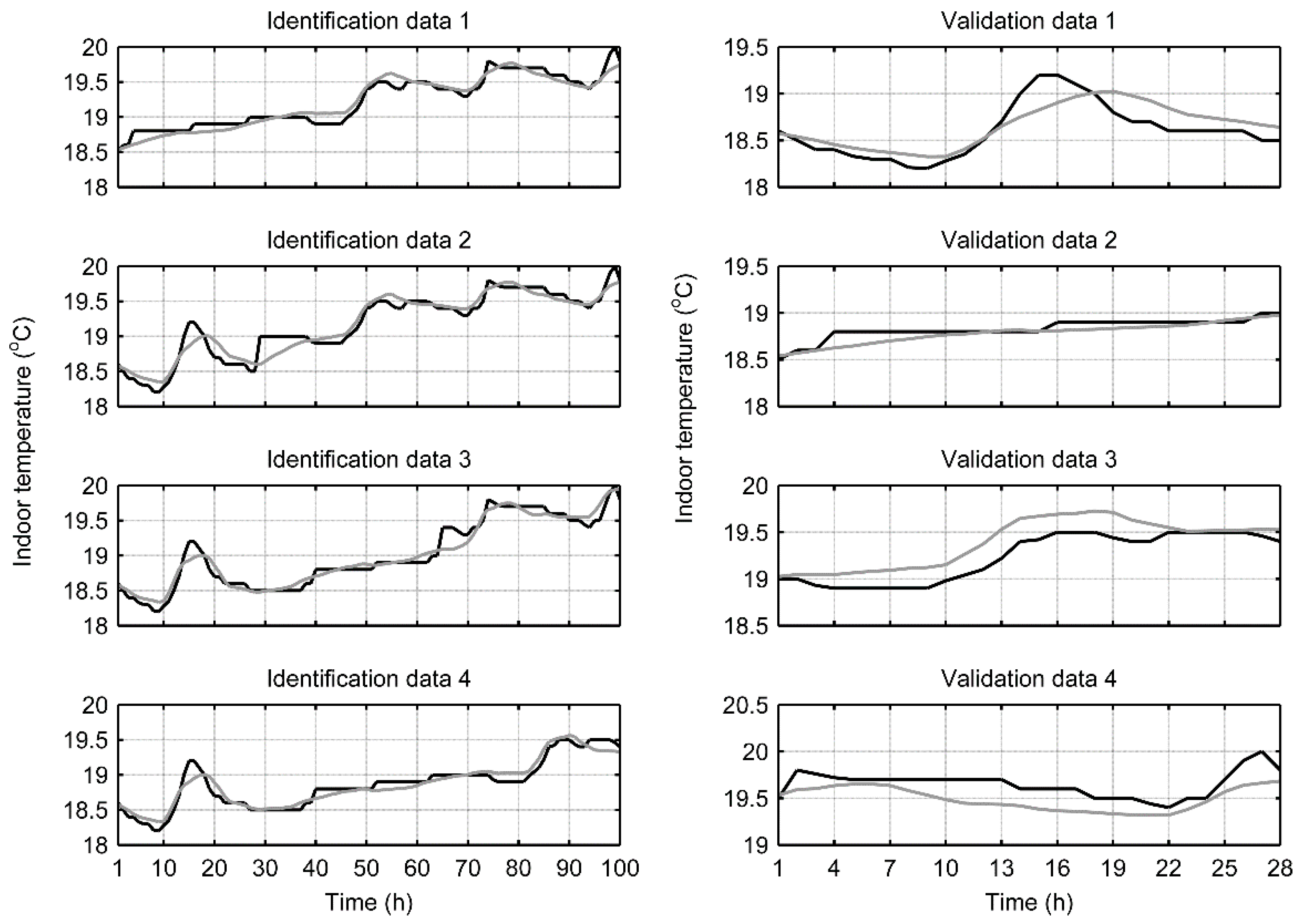
As the validation data might come from the middle of the data during the cross-validation (Figure 2), time discontinuity is introduced in the identification data when the remaining parts are merged as one. This is due to the fact that the dynamic model estimates future indoor temperature values based on past values of the indoor and outdoor temperature and heating power. However, this case only appears in two of four identification data and as can be seen in Figure 4, where an example of the cross-validation result with the modelling procedure (Figure 3) is presented with measured data from building A, it has no notable effect on the identification results. In this case, the average RMSE and r for four identification data sets were 0.10 °C and 0.97 respectively, and for four validation data sets 0.15 °C and 0.86, respectively.
As there were multiple positions for the indoor temperature measurement and three different C values, the results of the cross-validation were further examined to find the most representative indoor temperature measurement and the constant C value for each model structure in each building as presented in Figure 3. For each building, all indoor temperature measurement position and C value combinations for the same model structure were ranked according to NRMSE and r. NRMSE was used here to allow better comparison between different positions of the indoor temperature measurement inside the building as the temperature range could be different between them. For the lowest NRMSE value, the ranking started with the number 1. For the r, the highest value was ranked as number 1. Both the ranking results were then summed together to get the ranking order for each model structure with a different combination of the indoor temperature measurement position and C value. The most representative indoor temperature measurement position and C value combination for each model structure was the one that gave the lowest sum of two ranking numbers. Table 5 presents the cross-validation results for each building with the most representative indoor measurement position and C value combination.
It is worth noting that the model structures differ for all the studied buildings. In some buildings the more delayed power values give better results than the less delayed ones. This is also a clear indication that in some cases there exist significant delays between the measured indoor temperature and the heating power. The best results were achieved with data from building A where average RMSE and r for the validation data were 0.14 °C and 0.87 respectively (Table 5). The model performed most poorly in the building B, where only one indoor temperature measurement was available, indicating that the sensor position for the measurement has importance. For buildings D and E temperature sensors were located in the living rooms or hallways of the apartments. Still, good results were achieved in these buildings. Correlation was below 0.7 for all the studied buildings except for building A and this will be addressed in Section 4.3. At the same time, the average relative modelling error with the validation data sets and the model structures presented in Table 5 was below 5% for all buildings.
4.3. Generalizability Assessment
To investigate the generalizability of the model structures, mean RMSE and r values were calculated for each tested model structure using the simulation results of all five building data sets (Figure 3). This way the applicability of the same model structure to different buildings can be assessed as the best results might not be achieved with the same model structure (Table 5). Model structures were ranked according to mean RMSE and r values. This resulted in an individual ranking number for each model structure, where the lowest value represents the best performing model structure among those studied. As a result, nine of the best model structures according to the ranking procedure are presented in Table 6. The simplest model structure P1 is also included for comparison.
The differences between RMSE values are small among the ranked model structures including the model structure P1 (Table 6). For these model structures, the average relative modelling error for the 28-h prediction was below 5% in every building. Correlation was relatively low for all the listed model structures but differences between the best ranking ones were small. Correlation for P1 was lower and its standard deviation was significantly higher. Correlations were further analysed by calculating p-values for testing the null hypothesis that there is no correlation between the measured and modelled indoor temperature. Significant correlation was considered if the p-value was smaller than 0.05. For buildings A and D the p-value was smaller than 0.05 for all validation data sets. Building B had one validation data set with p-value greater than 0.05 indicating weak correlation. This is due to a very low measured indoor temperature value during one hour compared with previous and next hours. This could be a measurement error and if the value is changed to the mean value of adjacent hours, the correlation coefficient becomes 0.64 and p-value is then smaller than 0.05. For building C, there were two validation data sets that had p-values greater than 0.05. The low correlation for one validation data set can be explained by a sudden spike in the measured indoor temperature although there is no similar increase in the heating power and the model fails to model the change. Building E also had two validation data sets with p-values greater than 0.05. One general reason for the low correlations might be that the model output can be in higher resolution than the measured one, namely 0.1 °C. Therefore, in some cases low r values can be observed although the output of the model follows the measured values quite closely according to small RMSE. This is especially the case when the measured indoor temperature remains constant or it varies less than ±0.2 °C, which is the measurement accuracy for the typical indoor temperature sensors. In conclusion, while it is important to have high correlation between the measured and the modelled indoor temperature, in many cases the low correlation does not necessarily imply that the performance of the model is decreased.
The parameters along with their standard deviation for the best model structures in the case of building A are presented in Table 6. The values for the parameters a, b, x1, x2 and x3 are the mean values of the corresponding parameter with four identification data sets. For most of the best performing model structures the C value corresponds to light building structure (see Table 4). For the parameter a, the standard deviation is low among all the best performing models. Considering the model structures with the fewest parameters (P3 and P1), the standard deviation of the parameter a is six or seven times greater than the lowest standard deviation achieved. The smallest standard deviation for the parameter a can be achieved by the model structures with two heating power values, namely P1P3 and P1P8. When it comes to parameter b, the standard deviation as well as the value of the parameter varies more among the different model structures. Still, one of the smallest standard deviations is achieved with model P1P3.
The values and standard deviations of the parameters x1, x2 and x3 vary depending on the model structure. However, model structures with two heating power values produce smaller standard deviation for these parameters in general compared with model structures with three heating power values.
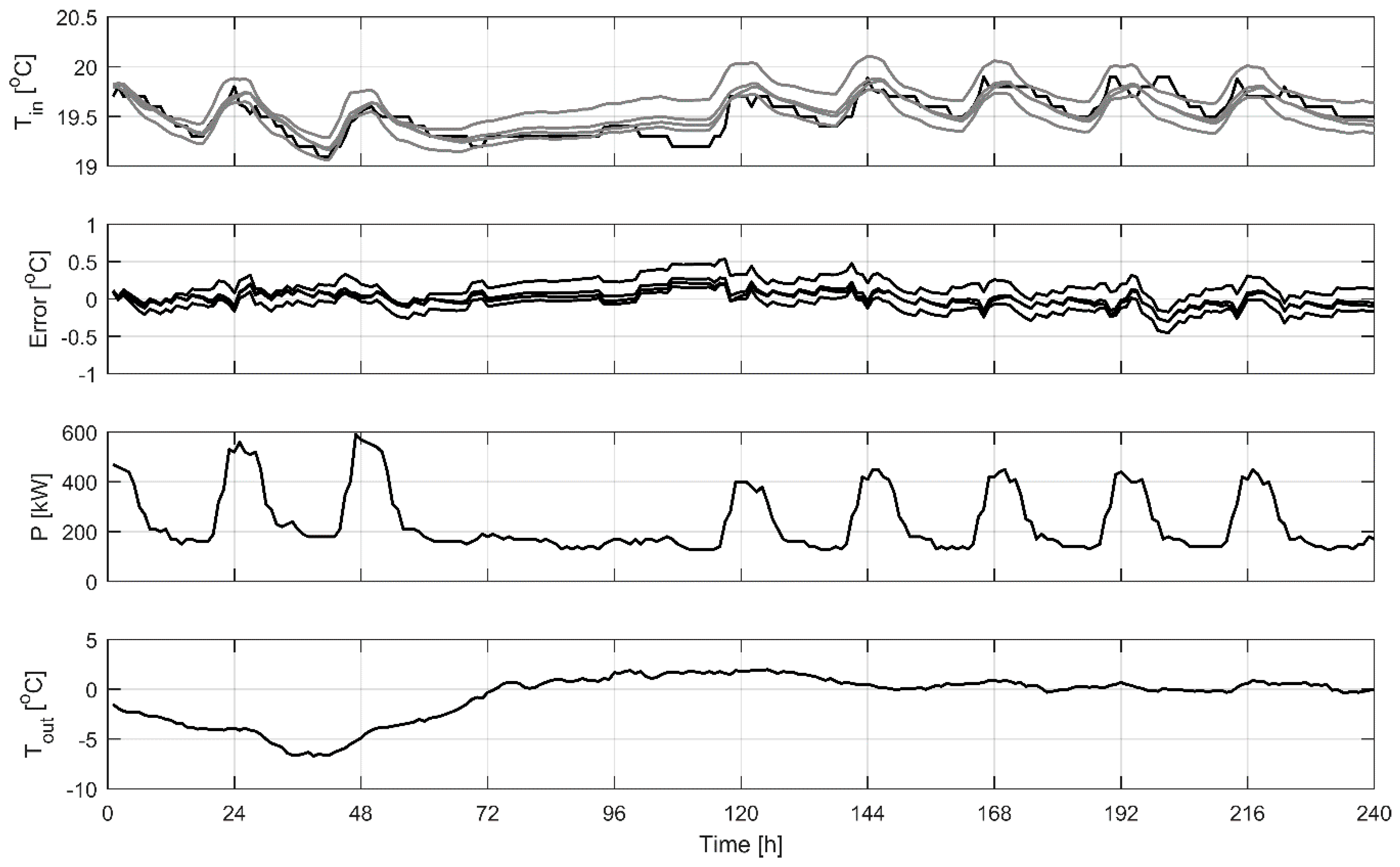
Model performance on a longer time horizon was tested for building A. Data for ten days after the 144-h period used for the cross-validation was utilized to simulate the indoor temperature. P1P3 model structure was used along with the same four sets of parameters that were estimated in the 4-fold cross-validation. The results can be seen in Figure 5. The model can estimate the indoor temperature accurately and the absolute modelling error is mainly under 0.5 °C for the whole simulation period. For the ten-day simulation period, RMSE was from 0.09 °C to 0.22 °C and r was from 0.76 to 0.88 depending on the parameters used. Those are comparable to the results achieved in cross-validation and presented in Figure 4. These results show that the model can accurately estimate the indoor temperature over longer periods of time.
For comparison, a state-of-the-art modelling approach was applied for building A. This model is a thermal network model presented in [52] and it was applied for the four identification and validation data sets. The model has two capacitances: one for the interior and the other for the walls. It also has three resistances: one between the interior and the walls, the second between the walls and the outside and the third for the heat flow through the windows and the doors. In total, the model has five physically interpretable parameters that needs to be estimated. Outputs of the model are the indoor temperature and the wall temperature. The upper and lower bounds for the estimated physical parameters were set as presented in Table 4 (minimum and maximum for U were set as 0 and 20). The resulted mean RMSE for the four identification and validation data sets were 0.28 ± 0.11 and 0.32 ± 0.23 respectively. The mean correlation coefficients for the four identification and validation data sets were 0.81 ± 0.11 and 0.34 ± 0.77 respectively. These are worse results when compared with the results with model P1P3 as presented in Figure 4. In addition, the wall temperature that needs to be estimated presents a challenge. In Brastein et al. [52], the wall temperature was measured but in real buildings this measurement is not available so it has to be estimated or at least initial guess needs to be made. With the identification and validation data of this study, the wall temperature can be estimated so that the model gives the best result with the measured indoor temperature. In prediction, however, initial guess for the wall temperature would be needed and it would be really hard to make. According to the results above, the initial guess for the wall temperature could be anything between 3.8 to 20 °C to achieve the best model performance. Also, the initial guesses and upper and lower bounds for the physical parameters has to be set correctly as they can have large impact on the final parameter estimates [52].
4.4. Error Analysis
Modelling error was further analysed by plotting the errors with four validation data sets as a function of time. Additionally, a histogram with normal distribution fit and a normal probability plot were used to check the statistical properties of the errors. Also, sample autocorrelation function in MATLAB® was applied to check if the modelling error can be considered as a white noise indicating appropriate complexity level of model structure.
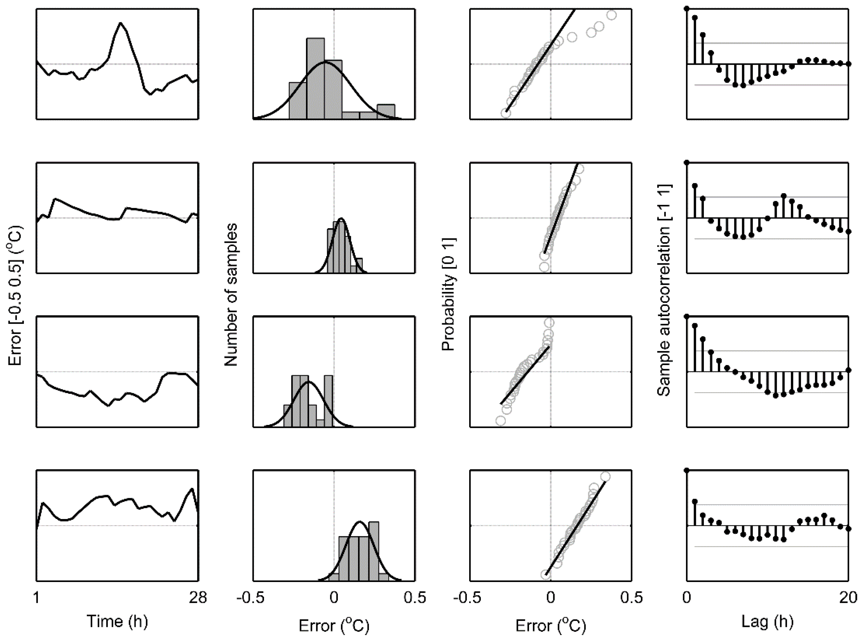
An example of the residual analysis with the measured data from building A is presented in Figure 6. The modelling errors are mainly similar to normal distribution. As the validation data contains only 28 data points, it could be expected that the error distribution would somewhat differ in comparison to theoretical normal distribution. In some error autocorrelation plots the 95% confidence bounds are slightly exceeded. However, in this case statistically significant error autocorrelations are mainly observed at low time lags.
At higher time lags, only few autocorrelations are outside the confidence bounds. In conclusion, the errors cannot be fully explained with white noise, but as the autocorrelations drop quickly and for the most part stays between the confidence bounds reasonable model performance can be assumed. Also, the modelling results with validation data (Figure 4) further support good model performance with respect to the applied performance criteria.
4.5. Uncertainty of the Outdoor Temperature Forecast
Outdoor temperature is an uncontrollable input to the developed model. In this work, validation has been done using the historical measured outdoor temperature. However, in reality an outdoor temperature forecast for predicting the indoor temperature would be required. Thus, the uncertainty of the forecast is an important issue to recognize as the outdoor temperature forecasts are not completely accurate [56]. Therefore, the effect of the uncertainty of the outdoor temperature forecast on the performance of the developed model was studied. Petersen and Bundgaard [56] analysed two years of outdoor temperature forecast data and corresponding actual outdoor temperature data. Based on that, the outdoor temperature forecast was modelled by sampling normally distributed values for the outdoor temperature for each of the 28-h validation data sets for building A. The normally distributed outdoor temperature values had a mean of the measured outdoor temperature value minus 0.4 °C and a standard deviation of 1.4 °C. In addition, outdoor temperature forecasts with a systematic error of 3 °C above or below the actual outdoor temperature for the 28-h validation periods were also examined for simulating the biased estimate. The results are presented in Figure 7. According to the sensitivity analysis with the above described data sets, the relative modelling error for Building A with the model structure P1P3 ranged from 0.3% to 1.6%. The relative modelling error using the actual outdoor temperature ranged from 0.3% to 0.9%. The results of the sensitivity analysis show, that even when the forecasted outdoor temperature deviates 3 °C from the actual outdoor temperature the magnitude of the modelling error stays mainly the same during the 28-h prediction horizon.
5. Applying the Model in Optimization of the Heat Demand
As presented in Section 4, by applying the same model structure in all five buildings an indoor temperature measurement that corresponds to the output of the model was found. It then follows that the model can be applied to predict these particular indoor temperatures in the buildings. By assuming that the current indoor temperature control systems in the buildings work as intended keeping the indoor temperatures at the set point level, the modelled indoor temperatures can be used to optimize the heat demand of the buildings. The modelled indoor temperature is then considered as representative indoor temperature for the building and can be altered between defined limits without compromising the living conditions. Above-mentioned assumptions mean that the indoor temperature in other parts of the building can also be considered being at permissible level.
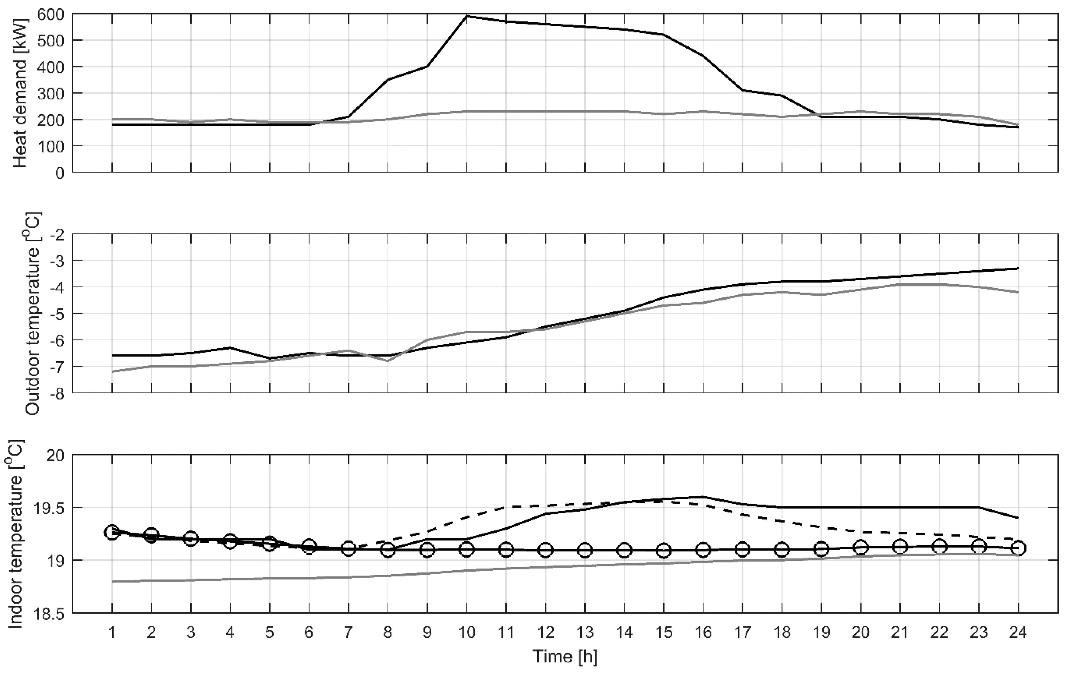
An example of what the optimization of the heat demand could mean in practice is presented in Figure 8 where heating power in building A has been set to lower level from normal operation conditions. Lower heating power level is taken from a reference day with a similar outdoor temperature profile. By applying the lower heating power level, the indoor temperature approaches the indoor temperature of the reference day which shows that the model can be used to predict and optimize the heat demand. In this example, the applied lower heating power can be considered the ‘optimized’ or ‘predicted’ heating power for the simulation period. Simulated indoor temperature with original heating power is also presented and the mean absolute error between the simulated and measured indoor temperature was 0.11 °C.
6. Discussion
It is worth noting that the modelling results presented in this article were achieved with a fairly small amount of measured data. Only 100 h of data was used for the estimation of the model parameters. Also, the data was recorded at the time when the buildings were in normal use. This included the actions of the automatic heating controls of the buildings. Furthermore, the energy used for hot water heating was not excluded from the heating power measurements, which could explain some of the modelling error. Although there were multiple indoor temperature sensors in the studied buildings, the final chosen sensor position may not be the optimal one. On that regard, it is remarkable that the indoor temperature measured inside an apartment could be used for the developed model as a representative temperature. Moreover, the C and U values were calculated using tabular values, which naturally introduces some error, and although three different C values were investigated the selected ones might not be the optimal values. Nevertheless, based on the modelling results, it can be concluded that this kind of data contains enough information to achieve acceptable model performance according to the presented testing criteria.
All the buildings studied in this research were large buildings, namely a school, a municipal hall and apartment buildings. Therefore, to assess the applicability of the model for smaller constructions, like detached houses, would require further studies. In [57], where detached houses were studied, significant consumption peaks in heat consumption due to domestic hot water were seen. In large buildings, the hot water consumption is largely in the noise. It is possible that the domestic hot water consumption will then have a more significant effect on the model performance in detached houses.
The presented model was identified without measuring the effects of the sun or wind to keep the number of model inputs as low as possible. However, Kapetanakis et al. [58] also found that the wind speed has no significant correlation to the heating load of the buildings. In the present study, the effect of the sun on the indoor temperature was investigated by calculating correlation between the modelling error RMSE and sunny weather. For all the buildings, the correlation was below 0.5 indicating no significant correlation. Furthermore, for four of the buildings correlation was also negative. In conclusion, there appeared to be no significant effect from the sun on the indoor temperature that the developed model could not account for. However, the inclusion of the solar heat gains as an input to the model and its impact on modelling accuracy should be investigated more thoroughly in future works. It should be noted that all the studied buildings are located in the northern hemisphere and relatively near the Arctic Circle. Therefore, the developed model can only be expected to work under similar conditions. In future works, the performance of the model in buildings under different climatic conditions should be studied.
Another challenging topic for future works is the application of the model in cases when the indoor temperature measurement is not available allowing even wider application of the model. Lack of the indoor temperature measurement is particularly the case in many older buildings. Also, the calculation of the physical model parameters needs information on building geometry that could be hard to gather for a large number of buildings, therefore more efficient ways to calculate or estimate these parameters are needed and will be looked into in future works.
Remarkably, the clear correlation between the measured indoor temperatures and its estimated values justifies the selected model structure. It then follows that, at least in large buildings, the indoor temperature variation can be modelled by the same parametrized version of the heat transfer equation (Equation (1)). These conclusions lay a foundation for the future studies where the developed model will be applied for the predictive optimization of the heat demand in a large number of buildings. This will include the optimization of the heating power of a single building and, more importantly, the focus then is on the simultaneous optimization and scheduling of multiple buildings, say from 200 to 500, enabled by the indicated generalizability potential of the presented modelling approach.
7. Conclusions
In this article, identification and validation of a novel dynamic model for the prediction and control of the indoor temperature in buildings was presented. The generalizability of the modelling approach was one of the main focus, this is why real measured data acquired from five different types of buildings were utilized in the model performance analysis. Use of easily available measurements and rough estimates for physical parameters are other important features of the studied model. Based on the simulations, relative modelling error during the 28-h prediction was below 5% with every building data set using the same model structure. In addition, the effect of uncertainty related to the outdoor temperature forecast affecting the performance of the model was minor. Results demonstrate a good modelling accuracy in various buildings using identical model structure despite few estimated physical parameters and simplicity of the model with respect to the total number of its parameters and inputs. Generalizable model structure allows to implement and adapt the model easily to a wide variety of different buildings as a part of city level energy optimization concepts.
Author Contributions
Conceptualization, P.H. and M.R.; Formal analysis, P.H. and M.R.; Funding acquisition, P.H., M.R. and K.L.; Investigation, P.H.; Methodology, P.H. and M.R.; Project administration, M.R. and K.L.; Software, P.H.; Supervision, K.L.; Validation, P.H.; Writing—original draft, P.H. and M.R.; Writing—review & editing, K.L.
Funding
This research was funded by the Finnish Funding Agency for Innovation (TEKES) through the project KLEI (40267/13) and the Academy of Finland through the project SEN2050 (287748).
Acknowledgments
The authors thank Oulun Energia Oy, Jyväskylän Energia Oy and Jyväskylän Vuokra-asunnot Oy for providing measurement data for this research and D.Sc. Marko Paavola for his valuable comments on the manuscript.
Conflicts of Interest
The authors declare no conflict of interest.
References
- Pérez-Lombard, L.; Ortiz, J.; Pout, C. A review on buildings energy consumption information. Energy Build. 2008, 40, 394–398. [Google Scholar] [CrossRef]
- Eisentraut, A.; Brown, A. Heating without Global Warming—Market Developments and Policy Considerations for Renewable Heat; IEA: Paris, France, 2014. [Google Scholar]
- Allegrini, J.; Orehounig, K.; Mavromatidis, G.; Ruesch, F.; Dorer, V.; Evins, R. A review of modelling approaches and tools for the simulation of district-scale energy systems. Renew. Sustain. Energy Rev. 2015, 52, 1391–1404. [Google Scholar] [CrossRef]
- Hietaharju, P.; Ruusunen, M. A concept for cutting peak loads in district heating. In Proceedings of the Automaatio XXI, Helsinki, Finland, 17–18 March 2015. [Google Scholar]
- Hietaharju, P.; Ruusunen, M. Peak Load Cutting in District Heating Network. In Proceedings of the 9th EUROSIM Congress on Modelling and Simulation, Oulu, Finland, 12–16 September 2016. [Google Scholar]
- Braun, J.E. Load Control Using Building Thermal Mass. J. Sol. Energy Eng. 2003, 125, 292–301. [Google Scholar] [CrossRef] [Green Version]
- Sun, Y.; Wang, S.; Xiao, F.; Gao, D. Peak load shifting control using different cold thermal energy storage facilities in commercial buildings: A review. Energy Convers. Manag. 2013, 71, 101–114. [Google Scholar] [CrossRef]
- Romanchenko, D.; Kensby, J.; Odenberger, M.; Johnsson, F. Thermal energy storage in district heating: Centralised storage vs. storage in thermal inertia of buildings. Energy Convers. Manag. 2018, 162, 26–38. [Google Scholar] [CrossRef]
- Kensby, J.; Trüschel, A.; Dalenbäck, J.-O. Potential of residential buildings as thermal energy storage in district heating systems—Results from a pilot test. Appl. Energy 2015, 137, 773–781. [Google Scholar] [CrossRef]
- Prívara, S.; Cigler, J.; Váňa, Z.; Oldewurtel, F.; Žáčeková, E. Use of partial least squares within the control relevant identification for buildings. Control Eng. Pract. 2013, 21, 113–121. [Google Scholar] [CrossRef]
- Zhao, H.; Magoulès, F. A review on the prediction of building energy consumption. Renew. Sustain. Energy Rev. 2012, 16, 3586–3592. [Google Scholar] [CrossRef]
- Kramer, R.; van Schijndel, J.; Schellen, H. Simplified thermal and hygric building models: A literature review. Front. Archit. Res. 2012, 1, 318–325. [Google Scholar] [CrossRef]
- Foucquier, A.; Robert, S.; Suard, F.; Stéphan, L.; Jay, A. State of the art in building modelling and energy performances prediction: A review. Renew. Sustain. Energy Rev. 2013, 23, 272–288. [Google Scholar] [CrossRef]
- Fraisse, G.; Viardot, C.; Lafabrie, O.; Achard, G. Development of a simplified and accurate building model based on electrical analogy. Energy Build. 2002, 34, 1017–1031. [Google Scholar] [CrossRef]
- Hudson, G.; Underwood, C.P. A simple building modelling procedure for MATLAB/SIMULINK. In Proceedings of the International Building Performance and Simulation Conference, Kyoto, Japan, 13–15 September 1999; Volume 2, pp. 777–783. [Google Scholar]
- Kossak, B.; Stadler, M. Adaptive thermal zone modeling including the storage mass of the building zone. Energy Build. 2015, 109, 407–417. [Google Scholar] [CrossRef]
- Royapoor, M.; Roskilly, T. Building model calibration using energy and environmental data. Energy Build. 2015, 94, 109–120. [Google Scholar] [CrossRef]
- Collotta, M.; Messineo, A.; Nicolosi, G.; Pau, G. A Dynamic Fuzzy Controller to Meet Thermal Comfort by Using Neural Network Forecasted Parameters as the Input. Energies 2014, 7, 4727–4756. [Google Scholar] [CrossRef] [Green Version]
- Gorni, D.; del Mar Castilla, M.; Visioli, A. An efficient modelling for temperature control of residential buildings. Build. Environ. 2016, 103, 86–98. [Google Scholar] [CrossRef]
- Gouda, M.M.; Danaher, S.; Underwood, C.P. Application of an Artificial Neural Network for Modelling the Thermal Dynamics of a Building’s Space and its Heating System. Math. Comput. Model. Dyn. Syst. 2002, 8, 333–344. [Google Scholar] [CrossRef]
- Huang, H.; Chen, L.; Hu, E. A neural network-based multi-zone modelling approach for predictive control system design in commercial buildings. Energy Build. 2015, 97, 86–97. [Google Scholar] [CrossRef]
- Kusiak, A.; Xu, G.; Zhang, Z. Minimization of energy consumption in HVAC systems with data-driven models and an interior-point method. Energy Convers. Manag. 2014, 85, 146–153. [Google Scholar] [CrossRef]
- Marvuglia, A.; Messineo, A.; Nicolosi, G. Coupling a neural network temperature predictor and a fuzzy logic controller to perform thermal comfort regulation in an office building. Build. Environ. 2014, 72, 287–299. [Google Scholar] [CrossRef]
- Mechaqrane, A.; Zouak, M. A comparison of linear and neural network ARX models applied to a prediction of the indoor temperature of a building. Neural Comput. Appl. 2004, 13, 32–37. [Google Scholar] [CrossRef]
- Mustafaraj, G.; Chen, J.; Lowry, G. Development of room temperature and relative humidity linear parametric models for an open office using BMS data. Energy Build. 2010, 42, 348–356. [Google Scholar] [CrossRef]
- Ruano, A.E.; Crispim, E.M.; Conceição, E.Z.E.; Lúcio, M.M.J.R. Prediction of building’s temperature using neural networks models. Energy Build. 2006, 38, 682–694. [Google Scholar] [CrossRef]
- Zamora-Martínez, F.; Romeu, P.; Botella-Rocamora, P.; Pardo, J. Towards Energy Efficiency: Forecasting Indoor Temperature via Multivariate Analysis. Energies 2013, 6, 4639–4659. [Google Scholar] [CrossRef] [Green Version]
- Attoue, N.; Shahrour, I.; Younes, R. Smart Building: Use of the Artificial Neural Network Approach for Indoor Temperature Forecasting. Energies 2018, 11, 395. [Google Scholar] [CrossRef]
- Fux, S.F.; Ashouri, A.; Benz, M.J.; Guzzella, L. EKF based self-adaptive thermal model for a passive house. Energy Build. 2014, 68, 811–817. [Google Scholar] [CrossRef]
- Gouda, M.M.; Danaher, S.; Underwood, C.P. Building thermal model reduction using nonlinear constrained optimization. Build. Environ. 2002, 37, 1255–1265. [Google Scholar] [CrossRef]
- Liao, Z.; Dexter, A.L. A simplified physical model for estimating the average air temperature in multi-zone heating systems. Build. Environ. 2004, 39, 1013–1022. [Google Scholar] [CrossRef]
- Underwood, C.P. An improved lumped parameter method for building thermal modelling. Energy Build. 2014, 79, 191–201. [Google Scholar] [CrossRef] [Green Version]
- Viot, H.; Sempey, A.; Mora, L.; Batsale, J.-C. Fast on-Site Measurement Campaigns and Simple Building Models Identification for Heating Control. Energy Procedia 2015, 78, 812–817. [Google Scholar] [CrossRef]
- Wang, S.; Xu, X. Simplified building model for transient thermal performance estimation using GA-based parameter identification. Int. J. Therm. Sci. 2006, 45, 419–432. [Google Scholar] [CrossRef]
- Wang, S.; Xu, X. Parameter estimation of internal thermal mass of building dynamic models using genetic algorithm. Energy Convers. Manag. 2006, 47, 1927–1941. [Google Scholar] [CrossRef]
- Braun, J.E.; Chaturvedi, N. An inverse gray-box model for transient building load prediction. HVAC R Res. 2002, 8, 73–99. [Google Scholar] [CrossRef]
- Kramer, R.; van Schijndel, J.; Schellen, H. Inverse modeling of simplified hygrothermal building models to predict and characterize indoor climates. Build. Environ. 2013, 68, 87–99. [Google Scholar] [CrossRef]
- Berthou, T.; Stabat, P.; Salvazet, R.; Marchio, D. Development and validation of a gray box model to predict thermal behavior of occupied office buildings. Energy Build. 2014, 74, 91–100. [Google Scholar] [CrossRef]
- Freire, R.Z.; Oliveira, G.H.C.; Mendes, N. Development of regression equations for predicting energy and hygrothermal performance of buildings. Energy Build. 2008, 40, 810–820. [Google Scholar] [CrossRef]
- Hazyuk, I.; Ghiaus, C.; Penhouet, D. Optimal temperature control of intermittently heated buildings using Model Predictive Control: Part I—Building modeling. Build. Environ. 2012, 51, 379–387. [Google Scholar] [CrossRef]
- Mateo, F.; Carrasco, J.J.; Sellami, A.; Millán-Giraldo, M.; Domínguez, M.; Soria-Olivas, E. Machine learning methods to forecast temperature in buildings. Expert Syst. Appl. 2013, 40, 1061–1068. [Google Scholar] [CrossRef] [Green Version]
- Moon, J.W.; Chung, M.H.; Song, H.; Lee, S.-Y. Performance of a Predictive Model for Calculating Ascent Time to a Target Temperature. Energies 2016, 9, 1090. [Google Scholar] [CrossRef]
- Prívara, S.; Cigler, J.; Váňa, Z.; Oldewurtel, F.; Sagerschnig, C.; Žáčeková, E. Building modeling as a crucial part for building predictive control. Energy Build. 2013, 56, 8–22. [Google Scholar] [CrossRef]
- Royer, S.; Thil, S.; Talbert, T.; Polit, M. A procedure for modeling buildings and their thermal zones using co-simulation and system identification. Energy Build. 2014, 78, 231–237. [Google Scholar] [CrossRef]
- Hilliard, T.; Swan, L.; Qin, Z. Experimental implementation of whole building MPC with zone based thermal comfort adjustments. Build. Environ. 2017, 125, 326–338. [Google Scholar] [CrossRef]
- Killian, M.; Mayer, B.; Kozek, M. Effective fuzzy black-box modeling for building heating dynamics. Energy Build. 2015, 96, 175–186. [Google Scholar] [CrossRef]
- Andersen, K.K.; Madsen, H.; Hansen, L.H. Modelling the heat dynamics of a building using stochastic differential equations. Energy Build. 2000, 31, 13–24. [Google Scholar] [CrossRef] [Green Version]
- Armstrong, P.R.; Leeb, S.B.; Norford, L.K. Control with building mass-Part I: Thermal response model. Trans. Am. Soc. Heat. Refrig. AIR Cond. Eng. 2006, 112, 449. [Google Scholar]
- Bacher, P.; Madsen, H. Identifying suitable models for the heat dynamics of buildings. Energy Build. 2011, 43, 1511–1522. [Google Scholar] [CrossRef] [Green Version]
- Madsen, H.; Holst, J. Estimation of continuous-time models for the heat dynamics of a building. Energy Build. 1995, 22, 67–79. [Google Scholar] [CrossRef]
- Thavlov, A.; Madsen, H. A non-linear stochastic model for an office building with air infiltration. Int. J. Sustain. Energy Plan. Manag. 2015, 7, 55–66. [Google Scholar] [CrossRef]
- Brastein, O.M.; Perera, D.W.U.; Pfeifer, C.; Skeie, N.-O. Parameter estimation for grey-box models of building thermal behaviour. Energy Build. 2018, 169, 58–68. [Google Scholar] [CrossRef]
- Hsu, D. Identifying key variables and interactions in statistical models of building energy consumption using regularization. Energy 2015, 83, 144–155. [Google Scholar] [CrossRef]
- Olsson Ingvarson, L.; Werner, S. Building mass used as short term heat storage. In Proceedings of the 11th International Symposium on District Heating and Cooling, Reykjavik, Iceland, 31 August–2 September 2008. [Google Scholar]
- Ministry of the Environment. The National Building Code of Finland. Available online: http://www.ym.fi/en-US/Land_use_and_building/Legislation_and_instructions/The_National_Building_Code_of_Finland (accessed on 23 April 2018).
- Petersen, S.; Bundgaard, K.W. The effect of weather forecast uncertainty on a predictive control concept for building systems operation. Appl. Energy 2014, 116, 311–321. [Google Scholar] [CrossRef]
- Bacher, P.; Madsen, H.; Nielsen, H.A.; Perers, B. Short-term heat load forecasting for single family houses. Energy Build. 2013, 65, 101–112. [Google Scholar] [CrossRef] [Green Version]
- Kapetanakis, D.-S.; Mangina, E.; Finn, D.P. Input variable selection for thermal load predictive models of commercial buildings. Energy Build. 2017, 137, 13–26. [Google Scholar] [CrossRef]
Figure 1.
Measured indoor temperature (Tin), heating power (P) and outdoor temperature (Tout) for the five different buildings. Two measurements from different locations are presented (one in black and the other in grey) for indoor temperature except for building B where only one measurement was available.

Figure 2.
The principle of the applied 4-fold cross-validation method. Measurement data is divided into four folds of equal lengths and one is used for the validation while the other ones are merged as an identification data for the parameter estimation.
Figure 2.
The principle of the applied 4-fold cross-validation method. Measurement data is divided into four folds of equal lengths and one is used for the validation while the other ones are merged as an identification data for the parameter estimation.
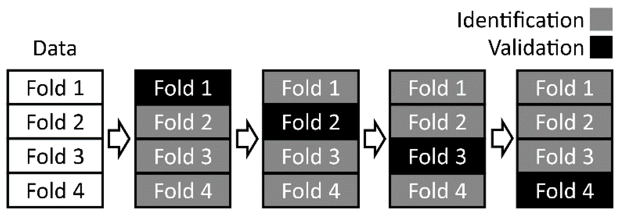
Figure 3.
An overview of the model identification and validation process. Cross-validation of the model structures is carried out for each building with all the combinations of indoor temperature measurements and C values and RMSE, NRMSE and r are calculated. For each model structures, the representative indoor temperature and C value combination is determined based on NRMSE and r. Generalizability is studied after all model structures are cross-validated in all of the buildings. The best model structures are determined based on RMSE and r.
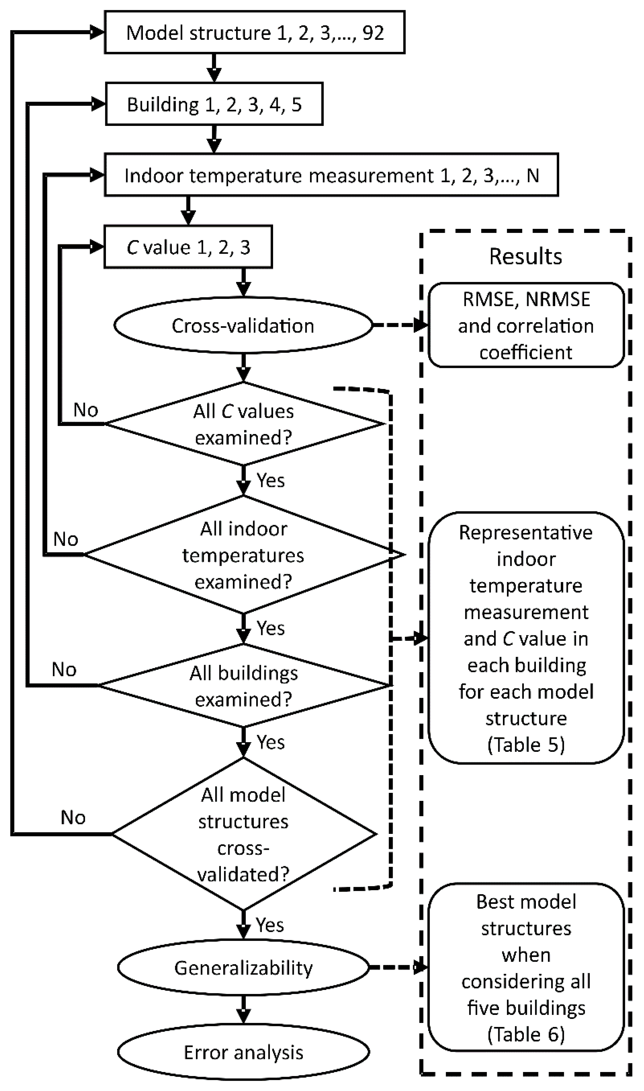
Figure 4.
Cross-validation results with data from building A with model structure P1P3. Black line is the measured indoor temperature and grey line is the estimated indoor temperature. For validation data sets, a 28-h ahead prediction was simulated with measured data. The RMSE for the identification data sets 1, 2, 3 and 4 was 0.09 °C, 0.13 °C, 0.11 °C and 0.09 °C, respectively, and for the validation data sets 1, 2, 3 and 4 it was 0.16 °C, 0.07 °C, 0.18 °C and 0.18 °C, respectively. Correlation coefficients for the identification data sets 1, 2, 3 and 4 were 0.97, 0.96, 0.98 and 0.96, respectively, and for the validation data sets 1, 2, 3 and 4 they were 0.84, 0.89, 0.94 and 0.79, respectively.

Figure 5.
Ten-day indoor temperature simulation for building A with model structure P1P3 utilizing the same four sets of parameters that were estimated in the 4-fold cross-validation. The measured (black line) and the estimated (grey lines) indoor temperatures are presented in the top. Error plots show the evolution of the modelling error during the ten-day simulation period.

Figure 6.
Analysis of the modelling error in case of model structure P1P3 with data from building A for four validation runs. Validation data set 1, 2, 3 and 4 are presented from the up to bottom row respectively. From left to right column: Modelling error (model output–measured); Histogram of the modelling error (grey bars) with normal distribution fit (black line); Normal probability plot for modelling errors; the sample autocorrelation function of the modelling error with 95% confidence bounds (grey lines).

Figure 7.
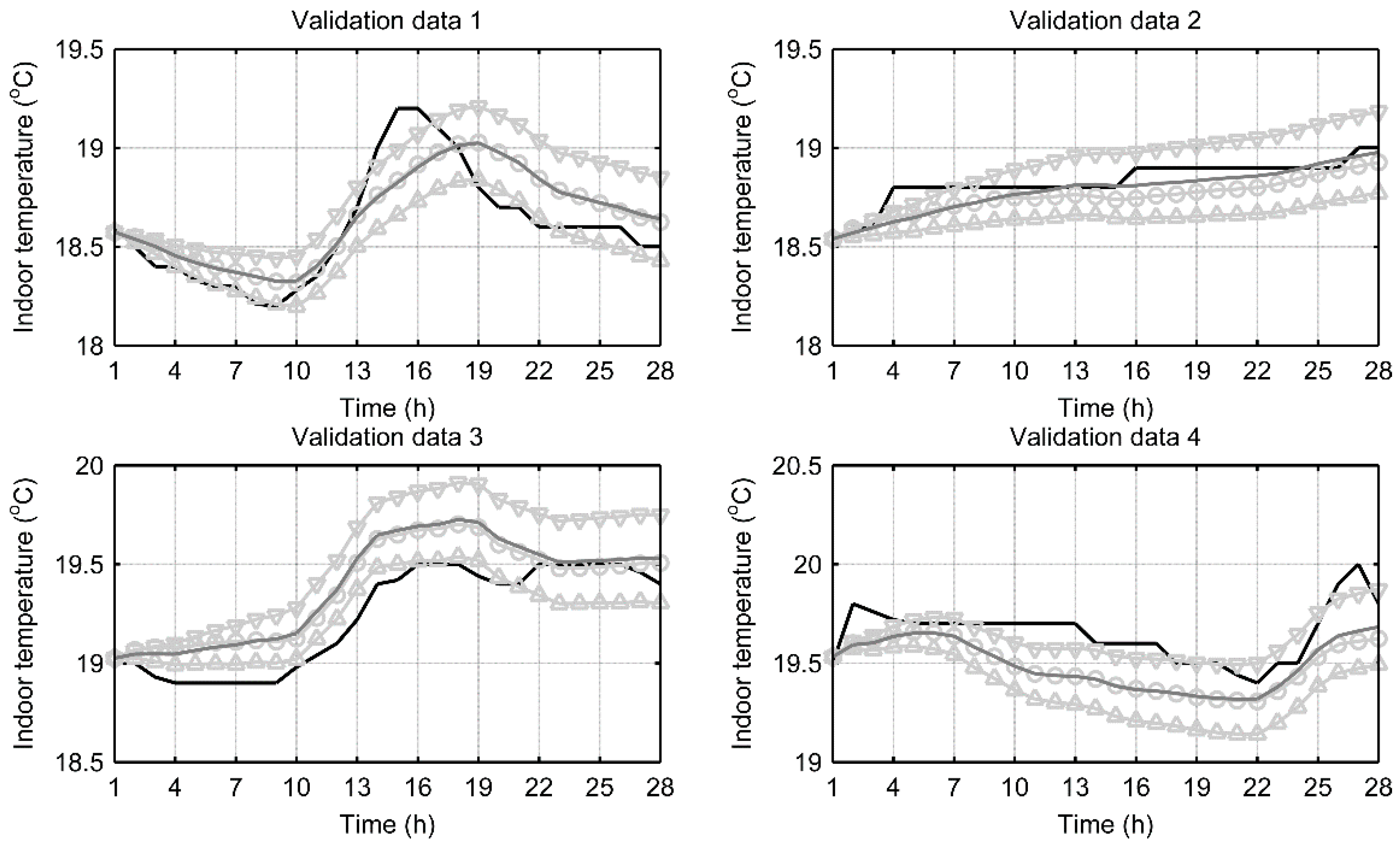
Sensitivity analysis of the indoor temperature prediction with simulated bias to the weather forecast in case of the model structure P1P3 with measured data from building A and four validation data sets. Black line is the measured indoor temperature and dark grey line is the indoor temperature prediction with measured outdoor temperature. Light grey line with circles is a representative example of the indoor temperature prediction with a normally distributed weather forecast. Light grey lines with upward and downward triangles are the simulated indoor temperature predictions using a weather forecast that contains a bias of 3 °C below or above the measured outdoor temperature respectively.
Figure 7.
Sensitivity analysis of the indoor temperature prediction with simulated bias to the weather forecast in case of the model structure P1P3 with measured data from building A and four validation data sets. Black line is the measured indoor temperature and dark grey line is the indoor temperature prediction with measured outdoor temperature. Light grey line with circles is a representative example of the indoor temperature prediction with a normally distributed weather forecast. Light grey lines with upward and downward triangles are the simulated indoor temperature predictions using a weather forecast that contains a bias of 3 °C below or above the measured outdoor temperature respectively.

Figure 8.
An example on the optimization of the heat demand in building A for a 24-h period. Upper: Measured heating powers for simulation day (black) and reference day (grey). Middle: Measured outdoor temperatures for simulation day (black) and reference day (grey). Lower: Measured (solid black) and simulated (dashed black) indoor temperature for simulation day and measured indoor temperature for reference day (grey). Black line with circles is the simulated indoor temperature for simulation day using reference day heating power.


Table 1.
Building characteristics.
| Building | Basal Area (m2) | Wall Area (m2) | Window Area (m2) | Floor Area (m2) | Volume (m3) | Construction Year | Building Type |
|---|---|---|---|---|---|---|---|
| A | 6700 | 4979 | 2418 | 13,400 | 79,781 | 2003–2004 | School |
| B | 633 | 1153 | 352 | 1903 | 8300 | 1982 | Apartment building |
| C | 1510 | 1274 | 142 | 3020 | 10,250 | 1983 | Municipal hall |
| D | 545 | 2000 | 400 | 3703 | 12,400 | 1972 | Apartment building |
| E | 993 | 2900 | 510 | 4200 | 15,617 | 2011 | Apartment building |
Table 2.
Measurement period, the number of different locations for indoor temperature sensors and the range of power and outdoor and indoor temperature measurement.
Table 2.
Measurement period, the number of different locations for indoor temperature sensors and the range of power and outdoor and indoor temperature measurement.
| Building | Measurement Period (mm/dd/yyyy) | Number of Sensor Locations | Range of Measurement Data | ||
|---|---|---|---|---|---|
| Heating Power (kW) | Outdoor Temperature (°C) | Indoor Temperature (°C) | |||
| A | 1/30/2014–2/5/2014 | 6 | 140–790 | −20.8–+0.5 | +16.1–+22.7 |
| B | 10/14/2014–10/20/2014 | 1 | 30–53 | −6.5–+3.8 | +14.3–+17.9 |
| C | 4/8/2014–4/14/2014 | 5 | 20–70 | −2.7–+9.0 | +19.3–+24.4 |
| D | 1/3/2015–1/8/2015 | 8 | 60–160 | −24.0–+0.4 | +20.2–+24.0 |
| E | 1/3/2015–1/8/2015 | 6 | 30–160 | −24.0–+0.4 | +21.2–+24.0 |
Table 3.
The overall heat loss coefficient values for the walls, roof and floor of the building in different years based on the National Building Code of Finland [55].
Table 3.
The overall heat loss coefficient values for the walls, roof and floor of the building in different years based on the National Building Code of Finland [55].
| Year | Walls (W/(m2·K)) | Roof (W/(m2·K)) | Floor (W/(m2·K)) | Building(s) Where Used |
|---|---|---|---|---|
| 1978 | 0.35 | 0.29 | 0.29 | B, C and D |
| 2003 | 0.25 | 0.16 | 0.20 | A |
| 2010 | 0.17 | 0.09 | 0.14 | E |
Table 4.
U and C values calculated from tabular values for buildings.
| Building | U (kW/K) | C (kJ/K) | ||
|---|---|---|---|---|
| Light | Medium | Heavy | ||
| A | 6.58 | 3,376,800 | 5,306,400 | 7,718,400 |
| B | 1.19 | 274,032 | 1,096,128 | 1,507,176 |
| C | 1.49 | 761,040 | 1,195,920 | 1,739,520 |
| D | 1.50 | 533,232 | 2,132,928 | 2,932,776 |
| E | 1.33 | 604,800 | 2,419,200 | 3,326,400 |
Table 5.
Cross-validation results with mean RMSE and r and their standard deviation. RMSE and r values were calculated by averaging the values of four identification/validation data sets. Parameters are presented as average values with their standard deviation over four identification data sets.
Table 5.
Cross-validation results with mean RMSE and r and their standard deviation. RMSE and r values were calculated by averaging the values of four identification/validation data sets. Parameters are presented as average values with their standard deviation over four identification data sets.
| Building (Model Structure) | Identification Data | Validation Data | Parameters 1 | |||||||
|---|---|---|---|---|---|---|---|---|---|---|
| RMSE ± stdRMSE (°C) | corr ± stdcorr | RMSE ± stdRMSE (°C) | corr ± stdcorr | C | a | b | x1 | x2 | x3 | |
| A (P2P3) | 0.12 ± 0.03 | 0.96 ± 0.01 | 0.14 ± 0.06 | 0.87 ± 0.07 | L | 0.92 ± 0.01 | 1.65 ± 0.15 | −0.64 ± 0.29 | 0.82 ± 0.31 | - |
| B (P2P3P7) | 0.48 ± 0.10 | 0.63 ± 0.14 | 0.42 ± 0.44 | 0.59 ± 0.29 | L | 0.96 ± 0.07 | 0.91 ± 1.53 | −0.15 ± 0.83 | 1.12 ± 1.25 | −0.85 ± 1.26 |
| C (P8) | 0.28 ± 0.12 | 0.45 ± 0.16 | 0.23 ± 0.20 | 0.67 ± 0.33 | L | 0.65 ± 0.10 | 7.06 ± 1.98 | - | - | - |
| D (P1P2) | 0.21 ± 0.01 | 0.74 ± 0.04 | 0.23 ± 0.06 | 0.68 ± 0.14 | M | 0.79 ± 0.06 | 4.50 ± 1.39 | 2.61 ± 1.92 | 0.06 ± 1.67 | - |
| E (P3) | 0.25 ± 0.01 | 0.69 ± 0.11 | 0.27 ± 0.11 | 0.65 ± 0.28 | M | 0.90 ± 0.03 | 2.09 ± 0.56 | - | - | - |
1 For C values, light (L), medium (M) or heavy (H) is used and the reader is referred to Table 4 for numerical values as well as for U values.
Table 6.
Modelling results with mean RMSE and r and their standard deviation with five buildings. RMSE and r values were calculated by averaging the values of the four identification/validation data sets for every building and then calculating the mean using values of all five buildings.
Table 6.
Modelling results with mean RMSE and r and their standard deviation with five buildings. RMSE and r values were calculated by averaging the values of the four identification/validation data sets for every building and then calculating the mean using values of all five buildings.
| Model Structure (Rank No.) | Identification Data | Validation Data | Parameters 1 | |||||||
|---|---|---|---|---|---|---|---|---|---|---|
| RMSE ± stdRMSE (°C) | corr ± stdcorr | RMSE ± stdRMSE (°C) | corr ± stdcorr | C | a | b | x1 | x2 | x3 | |
| P1P3 (1) | 0.25 ± 0.13 | 0.68 ± 0.18 | 0.27 ± 0.14 | 0.59 ± 0.19 | L | 0.92 ± 0.01 | 1.62 ± 0.12 | −0.32 ± 0.12 | 0.53 ± 0.09 | - |
| P3P6 (1) | 0.25 ± 0.13 | 0.69 ± 0.17 | 0.27 ± 0.11 | 0.59 ± 0.12 | L | 0.91 ± 0.02 | 1.86 ± 0.31 | −0.32 ± 0.08 | 0.44 ± 0.07 | - |
| P3 (2) | 0.28 ± 0.13 | 0.61 ± 0.17 | 0.28 ± 0.10 | 0.59 ± 0.15 | L | 0.51 ± 0.06 | 10.11 ± 1.29 | - | - | - |
| P1P8 (2) | 0.25 ± 0.13 | 0.69 ± 0.18 | 0.27 ± 0.13 | 0.58 ± 0.17 | L | 0.91 ± 0.01 | 1.76 ± 0.21 | −0.09 ± 0.06 | 0.28 ± 0.02 | - |
| P1P4P7 (2) | 0.24 ± 0.13 | 0.69 ± 0.18 | 0.29 ± 0.13 | 0.60 ± 0.18 | M | 0.95 ± 0.01 | 1.08 ± 0.11 | 0.13 ± 0.22 | −0.50 ± 0.22 | 0.65 ± 0.20 |
| P2P6P7 (2) | 0.24 ± 0.14 | 0.68 ± 0.15 | 0.26 ± 0.10 | 0.57 ± 0.12 | L | 0.80 ± 0.11 | 4.34 ± 2.18 | 0.63 ± 0.22 | −0.85 ± 0.29 | 0.67 ± 0.10 |
| P1P4 (3) | 0.24 ± 0.14 | 0.67 ± 0.17 | 0.28 ± 0.15 | 0.58 ± 0.15 | M | 0.88 ± 0.07 | 2.65 ± 1.36 | −0.25 ± 0.14 | 0.70 ± 0.02 | - |
| P2P3P6 (3) | 0.25 ± 0.12 | 0.73 ± 0.15 | 0.29 ± 0.12 | 0.59 ± 0.17 | L | 0.92 ± 0.01 | 1.63 ± 0.14 | 0.08 ± 0.25 | −1.04 ± 0.62 | 1.19 ± 0.45 |
| P3P7P8 (3) | 0.27 ± 0.13 | 0.69 ± 0.19 | 0.31 ± 0.13 | 0.61 ± 0.12 | L | 0.92 ± 0.01 | 1.69 ± 0.28 | 0.84 ± 0.34 | −1.18 ± 0.33 | 0.54 ± 0.05 |
| P1 (17) | 0.28 ± 0.14 | 0.61 ± 0.19 | 0.31 ± 0.15 | 0.46 ± 0.28 | L | 0.56 ± 0.07 | 9.23 ± 1.40 | - | - | - |
1 Parameters are presented for building A. For C values, light (L), medium (M) or heavy (H) is used and the reader is referred to Table 4 for numerical values as well as for U values.
© 2018 by the authors. Licensee MDPI, Basel, Switzerland. This article is an open access article distributed under the terms and conditions of the Creative Commons Attribution (CC BY) license (http://creativecommons.org/licenses/by/4.0/).
Share and Cite
MDPI and ACS Style
Hietaharju, P.; Ruusunen, M.; Leiviskä, K. A Dynamic Model for Indoor Temperature Prediction in Buildings. Energies 2018, 11, 1477. https://doi.org/10.3390/en11061477
AMA Style
Hietaharju P, Ruusunen M, Leiviskä K. A Dynamic Model for Indoor Temperature Prediction in Buildings. Energies. 2018; 11(6):1477. https://doi.org/10.3390/en11061477
Chicago/Turabian StyleHietaharju, Petri, Mika Ruusunen, and Kauko Leiviskä. 2018. "A Dynamic Model for Indoor Temperature Prediction in Buildings" Energies 11, no. 6: 1477. https://doi.org/10.3390/en11061477
Note that from the first issue of 2016, this journal uses article numbers instead of page numbers. See further details here.