Passivity-Based Robust Output Voltage Tracking Control of DC/DC Boost Converter for Wind Power Systems

Abstract

This paper exhibits a passivity-based robust output voltage controller for DC/DC boost converters for wind power system applications. The proposed technique has two features. The first one is to introduce a nonlinear disturbance observer for estimating the disturbances arising from the load and parameter variations. The second one is to derive a proportional-type passivity-based output voltage tracking controller incorporating the disturbance observer output, which simplifies the control algorithm by removing the use of tracking error integrators and an anti-windup algorithm. These two features constitute the useful closed-loop properties called the performance recovery and offset-free properties. Numerical simulation results confirm the efficacy of the proposed scheme, where a wind power system including the proposed controller is emulated using the PowerSIM software.

1. Introduction

A DC/DC boost converter driven by pulse-width modulation (PWM) provides an acceptable output voltage and current regulation performance with a power factor correction property. Because of these two beneficial properties, the DC/DC boost converter has wide industrial applications, including variable home appliances, electrical vehicles, and solar/wind power systems [1,2,3,4,5,6].

Conventionally, the cascade-type output voltage regulator has primarily been adopted for DC/DC boost converter control systems where the outer-loop voltage control output is used as the reference signal for the inner-loop current controller [7]. These inner- and outer-loops can be implemented using a simple proportional-integral (PI) controller with two degree of freedom for each loop, and the resulting closed-loop performance can be adjusted through the frequency domain using the Bode and Nyquist techniques [7,8]. The feedback-linearization technique was applied by combining the classical PI scheme and the converter parameter dependent feed-forward compensation terms, in which the PI gains are tuned for the cut-off frequency of the closed-loop transfer function using the converter parameters [7]. Thus, the parameter identification accuracy critically affects the closed-loop performance. The parameter dependency can be reduced by also incorporating the gain-scheduling techniques in the control algorithms, as in [9,10].

It was reported that closed-loop performance improvement could be achieved by applying several advanced techniques, such as deadbeat [11], predictive [12], sliding mode [13], adaptive [14,15], model predictive [16,17,18,19], and robust controllers [20]. However, these advanced techniques still have the parameter dependency problem, and, even in the case of an adaptive controller, knowledge of the true inductance value is required. Recently, a sliding mode technique [21] was devised through a multi-variable approach and efficiently alleviated the chattering effect. The upper and lower bounds of the disturbances should be found using a trial-and-error procedure, which determines the feed-forward compensation terms dominating the disturbances coming from the load and parameter variations.

This paper presents a robust output voltage tracking controller for DC/DC boost converters, which considers the nonlinear dynamic behavior and model–plant mismatches arising from load and parameter variations. The proposed technique is devised through a multi-variable approach in the port-controlled Hamiltonian (PCH) framework introduced in [22]. This study made three contributions. First, a nonlinear disturbance observer (DOB) was constructed to exponentially estimate the disturbances given in the perturbed converter dynamical equations. Second, a proportional-type output voltage controller was devised by solving a partial differential equation (PDE) for the desired closed-loop energy function, including the DOB state variables. Third, it is rigorously proven that the closed-loop system driven by the proposed technique ensures two beneficial properties called the performance recovery and offset-free properties without the use of the tracking error integrators. These three contributions could simplify the control algorithms by: (1) reducing the dependency on converter information, such as the parameters and load current; and (2) removing the tracking error integral actions with anti-windup algorithms, which is a stark contrast to previous studies. Realistic simulations verify the effectiveness of the proposed technique by implementing a wind power system comprised of a wind turbine, permanent magnet synchronous generator (PMSG), and three-phase diode rectifier.

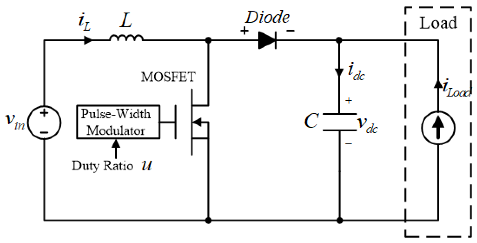
2. DC/DC Boost Converter Nonlinear Dynamics

The application of the averaging technique to the DC/DC boost converter depicted in Figure 1 leads to the nonlinear differential equations as [7]

$$\begin{array}{ccc}\hfill L{\dot{i}}_L(t)& =& -(1-u(t))v_{dc}(t)+v_{in}(t),\hfill \end{array}$$

(1)

$$\begin{array}{ccc}\hfill C{\dot{v}}_{dc}(t)& =& (1-u(t))i_L(t)-i_{Load}(t),\forall t\ge 0,\hfill \end{array}$$

(2)

where the averaged inductor current of $i_L(t)$ and output voltage of $v_{dc}(t)$ are treated as the state variables, and the duty ratio of $u(t)$ acts as the control input constrained in the closed-interval of $[0,1]$. The inductance and capacitance values are denoted as L and C, respectively. The input DC source voltage of $v_{in}(t)$ comes from a wind power system comprised of a wind turbine, PMSG, and rectifier, and the load current of $i_L(t)$ acts as the external disturbance.

Considering the wind power system implementations, the following assumptions are made:

• The true inductance and capacitance values are unknown but their nominal values, denoted as $L_0$ and $C_0$, are known.
• The input DC source voltage of $v_{in}(t)$ is time-varying but unknown except for its initial value, i.e., $v_{in,0}=v_{in}(0)$ is known.
• The load current of $i_{Load}(t)$ is unknown and time-varying.
• The inductor current of $i_L(t)$ and output voltage of $v_{dc}(t)$ are available for feedback.

The converter dynamics of Equations (1) and (2) show that the output voltage tracking control problem is not trivial because of the nonlinear terms presented in the inductor and output voltage dynamics and the unstable zero-dynamics. This paper tackles this difficulty by combining the passivity approach introduced in [22] and DOB techniques. For details, see the following section.

3. Output Voltage Tracking Controller Design

This section develops an output voltage tracking algorithm that allows the closed-loop output voltage behavior to be convergent to the low-pass filter (LPF) dynamics as

$$\begin{array}{c}\hfill \frac{V_{dc}(s)}{V_{dc,ref}(s)}=\frac{{\omega }_{vc}}{s+{\omega }_{vc}},\forall s\in \mathbb{C},\end{array}$$

(3)

with a desired cut-off frequency of ${\omega }_{vc}>0$, where $V_{dc}(s)$ and $V_{dc,ref}(s)$ stand for the Laplace transforms of $v_{dc}(t)$ and $v_{dc,ref}(t)$, respectively. For this purpose, Section 3.1 analyzes the open-loop stability using a positive-definite energy function, which is used to constitute a PDE. Section 3.2 designs the PDE using the open-loop and closed-loop energy functions and proposes an output voltage tracking controller for solving the resulting PDE. Finally, Section 3.3 presents two useful closed-loop properties, called the performance recovery and offset-free properties, by analyzing the closed-loop dynamics.

3.1. Open-Loop Stability Analysis

First, to remove the true parameter dependency, rewrite the nonlinear dynamics of Equations (1) and (2) using the nominal converter parameters of $L_0$ and $C_0$ with the initial input DC source voltage of $v_{in,0}$ as:

$$\begin{array}{ccc}\hfill L_0{\dot{i}}_L(t)& =& -(1-u(t))v_{dc}(t)+v_{in,0}+d_{L,o}(t),\hfill \end{array}$$

(4)

$$\begin{array}{ccc}\hfill C_0{\dot{v}}_{dc}(t)& =& (1-u(t))i_L(t)+d_{v,o}(t),\forall t\ge 0,\hfill \end{array}$$

(5)

with $d_{L,o}(t)$ and $d_{v,o}(t)$ being unknown lumped disturbances caused by the model–plant mismatches, which can be written in a vector form:

$$\begin{array}{c}\hfill \mathbf{M}\dot{\mathbf{x}}(t)=\mathbf{J}(u(t)){\mathbf{M}}^{-1}\nabla H(\mathbf{x}(t))+\mathbf{g}+{\mathbf{d}}_o(t),\forall t\ge 0,\end{array}$$

(6)

where the state vector of $\mathbf{x}(t)$ is defined as $\mathbf{x}(t):={\left[\begin{array}{cc}{i}_L(t)& v_{dc}(t)\end{array}\right]}^T$, $\nabla H(\mathbf{x}(t))$ denotes the gradient of the open-loop energy function of $H(\mathbf{x}(t))$ given by $H(\mathbf{x}(t)):=\frac{1}{2}{\mathbf{x}}^T(t)\mathbf{M}\mathbf{x}(t)$, $\forall t\ge 0$ with the positive definite matrix of $\mathbf{M}:=$ diag$\left\{L_0,C_0\right\}$, and the rest of the system matrices are defined as

$$\begin{array}{c}\hfill \mathbf{J}(u(t)):=\left[\begin{array}{cc}0& -(1-u(t))\\ (1-u(t))& 0\end{array}\right],\mathbf{g}:=\left[\begin{array}{c}{v}_{in,0}\\ 0\end{array}\right],{\mathbf{d}}_o(t):=\left[\begin{array}{c}{d}_{L,o}(t)\\ d_{v,o}(t)\end{array}\right],\forall t\ge 0.\end{array}$$

The open-loop stability can easily be seen using the open-loop energy function of $H(\mathbf{x}(t))$ and the state equation of Equation (6) as

$$\begin{array}{ccc}\hfill \dot{H}(\mathbf{x}(t))& =& \nabla H^T(\mathbf{x}(t))\dot{\mathbf{x}}(t)={\mathbf{x}}^T(t)\mathbf{M}\left({\mathbf{M}}^{-1}\left[\mathbf{J}(u(t)){\mathbf{M}}^{-1}\nabla H(\mathbf{x}(t))+\mathbf{g}+{\mathbf{d}}_o(t)\right]\right)\hfill \\ & =& {\mathbf{x}}^T(t)\left(\mathbf{J}(u(t))\mathbf{x}(t)+\mathbf{g}+{\mathbf{d}}_o(t)\right)={\mathbf{x}}^T(t)(\mathbf{g}+{\mathbf{d}}_o(t)),\forall t\ge 0,\hfill \end{array}$$

which shows the passivity for the input-output mapping of $(\mathbf{g}+{\mathbf{d}}_o(t))\mapsto \mathbf{x}(t)$.

3.2. Controller Design

The control problem for the target dynamics of Equation (3) can be solved by deriving a control law that forces the closed-loop output voltage trajectory of $v_{dc}(t)$ to exponentially converge to the desired trajectory of $v_{dc}^{\ast }(t)$ governed by

$$\begin{array}{c}\hfill {\dot{v}}_{dc}^{\ast }(t)={\omega }_{vc}\left(v_{dc,ref}(t)-v_{dc}^{\ast }(t)\right),\forall t\ge 0,\end{array}$$

(7)

because the dynamical Equation (7) is the inverse Laplace transform of Equation (3). To this end, define the tracking error vector as $\tilde{\mathbf{x}}(t):={\mathbf{x}}_{ref}(t)-\mathbf{x}(t)={\left[\begin{array}{cc}{\tilde{i}}_L(t)& {\tilde{v}}_{dc}^{\ast }(t)\end{array}\right]}^T$ with the reference vector of ${\mathbf{x}}_{ref}(t):={\left[\begin{array}{cc}{i}_{L,ref}(t)& v_{dc}^{\ast }(t)\end{array}\right]}^T$, where $i_{L,ref}(t)$ refers to the inductor current reference determined later. Then, the tracking error dynamics are obtained as

$$\begin{array}{ccc}\hfill \mathbf{M}\dot{\tilde{\mathbf{x}}}(t)& =& \mathbf{M}({\dot{\mathbf{x}}}_{ref}(t)-\dot{\mathbf{x}}(t))\hfill \\ & =& -\mathbf{J}(u(t)){\mathbf{M}}^{-1}\nabla H(\mathbf{x}(t))-\mathbf{g}+\mathbf{d}(t),\forall t\ge 0,\hfill \end{array}$$

(8)

where the disturbance vector of $\mathbf{d}(t)$ is defined as $\mathbf{d}(t):=\mathbf{M}{\dot{\mathbf{x}}}_{ref}(t)-{\mathbf{d}}_o(t)$, $\forall t\ge 0$. Now, consider the closed-loop positive definite energy function given by

$$\begin{array}{c}\hfill H_{cl}(\tilde{\mathbf{x}}(t)):=\frac{1}{2}{\tilde{\mathbf{x}}}^T(t)\mathbf{M}\tilde{\mathbf{x}}(t),\forall t\ge 0,\end{array}$$

(9)

which gives its time-derivative along the trajectory of Equation (8):

$$\begin{array}{ccc}\hfill {\dot{H}}_{cl}(\tilde{\mathbf{x}}(t))& =& \nabla H_{cl}^T(\tilde{\mathbf{x}}(t))\dot{\tilde{\mathbf{x}}}(t)\hfill \\ & =& \nabla H_{cl}^T(\tilde{\mathbf{x}}(t)){\mathbf{M}}^{-1}\left(-\mathbf{J}(u(t)){\mathbf{M}}^{-1}\nabla H(\mathbf{x}(t))-\mathbf{g}+\mathbf{d}(t)\right),\forall t\ge 0.\hfill \end{array}$$

(10)

Through a further analysis using Lemma 1, it can be proven that a useful inequality of

$$\begin{array}{c}\hfill {\dot{H}}_{cl}(\tilde{\mathbf{x}}(t))\le -{\alpha }_{cl}{H}_{cl}(\tilde{\mathbf{x}}(t))+{\tilde{\mathbf{d}}}^T(t)\tilde{\mathbf{x}}(t),\forall t\ge 0,\end{array}$$

(11)

holds for some ${\alpha }_{cl}>0$ where $\tilde{\mathbf{d}}(t):=\mathbf{d}(t)-\widehat{\mathbf{d}}(t)$ with $\widehat{\mathbf{d}}(t)={\left[\begin{array}{cc}{\widehat{d}}_L(t)& {\widehat{d}}_v(t)\end{array}\right]}^T$ being the estimated disturbance vector, $\forall t\ge 0$, if the PDE of

$$\begin{array}{c}\hfill -\mathbf{J}(u(t)){\mathbf{M}}^{-1}\nabla H(\mathbf{x}(t))-\mathbf{g}=\left({\mathbf{J}}_{cl}(u(t))-{\mathbf{R}}_{cl}\right){\mathbf{M}}^{-1}\nabla H_{cl}(\tilde{\mathbf{x}}(t))-\widehat{\mathbf{d}}(t),\forall t\ge 0,\end{array}$$

(12)

is solvable for some skew-symmetric matrix of ${\mathbf{J}}_{cl}(u(t))$ and positive definite matrix of ${\mathbf{R}}_{cl}$.

The PDE of Equation (12) can be solved using the proposed control law $u(t)$, with the inductor current reference $i_{L,ref}(t)$ given by

$$\begin{array}{ccc}\hfill u(t)& =& \frac{1}{v_{dc}^{\ast }(t)}\left(L_0{k}_{cc}{\tilde{i}}_L(t)+v_{dc}^{\ast }(t)-v_{in,0}+{\widehat{d}}_L(t)\right),\hfill \end{array}$$

(13)

$$\begin{array}{ccc}\hfill i_{L,ref}(t)& =& \frac{1}{1-u(t)}\left(C_0{k}_{vc}{\tilde{v}}_{dc}^{\ast }(t)+{\widehat{d}}_v(t)\right),\forall t\ge 0,\hfill \end{array}$$

(14)

with ${\mathbf{J}}_{cl}(u(t))=\mathbf{J}(u(t))$ and ${\mathbf{R}}_{cl}=$ diag$\left\{L_0{k}_{cc},C_0{k}_{vc}\right\}$ for any given tuning parameters of $k_{cc}>0$ and $k_{vc}>0$. Meanwhile, the estimated disturbance vector of $\widehat{\mathbf{d}}(t)$ is given by

$$\begin{array}{c}\hfill \widehat{\mathbf{d}}(t)=\mathbf{z}(t)+\mathbf{L}\mathbf{M}\tilde{\mathbf{x}}(t),\forall t\ge 0,\end{array}$$

(15)

with the diagonal DOB gain matrix of $\mathbf{L}=$ diag$\{l_{cc},l_{vc}\}>\mathbf{0}$. The DOB state vector of $\mathbf{z}(t)$ is updated as

$$\begin{array}{c}\hfill \dot{\mathbf{z}}(t)=-\mathbf{L}\mathbf{z}(t)-{\mathbf{L}}^2\mathbf{M}\tilde{\mathbf{x}}(t)+\mathbf{L}\left(\mathbf{J}(u(t))\mathbf{x}(t)+\mathbf{g}\right),\forall t\ge 0,\end{array}$$

(16)

Lemma 1 presents a beneficial inequality of Equation (11) to derive a closed-loop property through investigating the closed-loop energy function behavior driven by the proposed controller of Equation (13) with the inductor current reference of Equation (14). The proof is given in the Appendix A.

Lemma 1.

For any given $k_x>0$, $x=cc,vc$, the proposed controller of Equation (13) with the inductor current reference of Equation (14) solves the PDE of Equation (12) such that the inequality of Equation (11) holds true.

3.3. Closed-Loop Property Analysis

This subsection rigorously analyzes the closed-loop properties. First, Theorem 1 derives a closed-loop property, called the performance recovery property, which includes the DOB output of Equation (15) and the DOB state equation of Equation (16) based on the inequality of Equation (11) derived by Lemma 1. The Appendix A presents the proof of Theorem 1.

Theorem 1.

Under the assumption of Lemma 1, for any $k_x>0$ and $l_x$, $x=cc,vc$, the proposed controller of Equation (13) with the inductor current reference of Equation (14) and DOB of Equations (15) and (16) ensures strict passivity for the input–output mapping:

$$\begin{array}{c}\hfill \mathit{w}(t)\mapsto \mathit{y}(t),\end{array}$$

(17)

where $\mathit{w}(t):={\left[\begin{array}{ccc}0& 0& {(\Gamma \dot{\mathit{d}}(t))}^T\end{array}\right]}^T$ and $\mathit{y}(t):={\left[\begin{array}{cc}{\tilde{\mathit{x}}}^T(t)& {\tilde{\mathit{d}}}^T(t)\end{array}\right]}^T$ for some $\Gamma ={\Gamma }^T>\mathbf{0}$, $\forall t\ge 0$.

The proof of Theorem 1 can be accomplished by showing that the composite-type positive-definite function of $V(t)$ defined as

$$\begin{array}{c}\hfill V(\tilde{\mathbf{x}}(t),\tilde{\mathbf{d}}(t)):=H_{cl}(\tilde{\mathbf{x}}(t))+\frac{1}{2}{\tilde{\mathbf{d}}}^T(t)\Gamma \tilde{\mathbf{d}}(t),\forall t\ge 0,\end{array}$$

(18)

with a positive definite weighting matrix of $\Gamma$ gives

$$\begin{array}{c}\hfill \dot{V}(\tilde{\mathbf{x}}(t),\tilde{\mathbf{d}}(t))\le -\beta V(\tilde{\mathbf{x}}(t),\tilde{\mathbf{d}}(t))+{\mathbf{w}}^T(t)\mathbf{y}(t),\forall t\ge 0,\end{array}$$

(19)

for some $\beta >0$. For details, see the Appendix A. The resulting inequality of Equation (19) implies that the closed-loop system driven by the proposed control algorithm exponentially recovers the target output voltage tracking performance of Equation (7) as the disturbance vector of $\mathbf{d}(t)$ exponentially reaches its steady state, i.e., $v_{dc}(t)\to v_{dc}^{\ast }(t)$ as $\dot{\mathbf{d}}(t)\to \mathbf{0}$, exponentially.

Theorem 2 shows that the closed-loop system does not suffer from an offset error despite the absence of the tracking error integrators in the proposed controller, thanks to the DOB dynamics of Equations (15) and (16). This property is called the offset-free property to simplify the controller by removing the additional anti-windup algorithms. The proof is given in the Appendix A.

Theorem 2.

The closed-loop system controlled by the proposed control algorithm of Equations (13)–(16) always removes the output voltage steady state error, i.e, $v_{dc}(\infty )=v_{dc,ref}(\infty )$ where $v_{dc}(\infty )$ and $v_{dc,ref}(\infty )$ denote the steady states of $v_{dc}(t)$ and $v_{dc,ref}(t)$, respectively.

4. Simulation Results

This section describes the simulation results of a wind power system that includes the DC/DC boost converter to numerically demonstrate the effectiveness of the proposed technique. Section 4.1 gives the simulation setup. The numerical verification results are presented in Section 4.2. Section 4.3 concludes this section by discussing the numerical verification results.

4.1. Simulation Setup

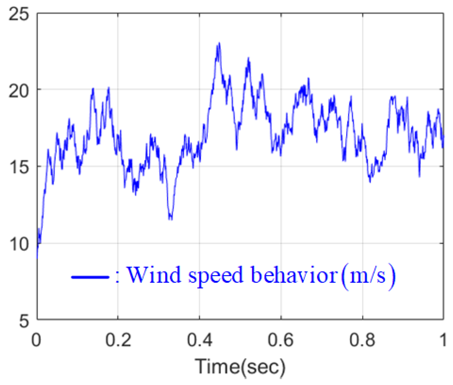
The wind power system was emulated by the powerSIM (PSIM) software using its wind turbine and permanent magnet synchronous machine (PMSM) model. The following values were selected for the nominal output power, inertia, base wind and rotational speed, and initial rotational speed of the wind turbine: 10-kW, $0.1{\mathrm{kg}·\mathrm{m}}^2$, $20\mathrm{m}/\mathrm{s}$, 50 rpm, and 10 rpm, respectively. The PMSM parameters were chosen as $R_s=0.099\Omega$ (stator resistance), $L_d=L_q=4.07\mathrm{mH}$ (d-q inductances), ${\lambda }_{PM}=0.3166\mathrm{Wb}$ (flux), $P=40$ (number of poles), $J=0.12{\mathrm{kg}·\mathrm{m}}^2$ (inertia), $B=0.000425\mathrm{Nm}/\mathrm{rad}/\mathrm{s}$ (viscous damping). The Weibull distribution-based wind model [23] was used to randomly determine the wind speed for the wind turbine, which is shown in Figure 2. As components of the DC/DC boost converter, the inductance of L and the capacitance of C were selected as

$$\begin{array}{c}\hfill L=460\mu H,C=470\mu F,\end{array}$$

(20)

and their nominal values were determined to be

$$\begin{array}{c}\hfill L_0=0.5L,C_0=1.5C,\end{array}$$

(21)

to take the model–plant mismatches into account, where the input DC source voltage was supplied by the PMSM with a three-phase diode rectifier. Figure 3 shows the emulated wind power system configuration, whose output DC-link voltage of $v_{dc}(t)$ was controlled by the DC/DC boost converter. The control algorithms were implemented using the dynamic link library (DLL) block written in the C language, where the pulse-width modulation (PWM) and control periods were chosen to be synchronized to $0.1$ ms.

For comparison, the feedback linearization (FL) technique was considered [7], which is given as

$$\begin{array}{c}\hfill u(t)=2L_0{\omega }_{cc}{\tilde{i}}_L(t)+L_0{\omega }_{cc}^2{\int }_0^t{\tilde{i}}_L(\tau )d\tau ,\forall t\ge 0,\end{array}$$

(22)

with the inductor current tracking error of ${\tilde{i}}_L(t):=i_{L,ref}(t)-i_L(t)$, $\forall t\ge 0$, where the inductor current reference of $i_{L,ref}(t)$ is updated by the outer-loop voltage regulator as

$$\begin{array}{c}\hfill i_{L,ref}(t)=2C_0{\omega }_{vc}{\tilde{v}}_{dc}(t)+C_0{\omega }_{vc}^2{\int }_0^t{\tilde{v}}_{dc}(\tau )d\tau ,\forall t\ge 0,,\end{array}$$

(23)

with the output voltage tracking error of ${\tilde{v}}_{dc}(t):=v_{dc,ref}(t)-v_{dc}(t)$, $\forall t\ge 0$. The resulting closed-loop system controlled by the FL technique gives the closed-loop transfer function

$$\begin{array}{c}\hfill \frac{I_L(s)}{I_{L,ref}(s)}\approx \frac{{\omega }_{cc}}{s+{\omega }_{cc}},\frac{V_{dc}(s)}{V_{dc,ref}(s)}\approx \frac{{\omega }_{vc}}{s+{\omega }_{vc}},\forall s\in \mathbb{C},\end{array}$$

(24)

as long as the nominal parameters of $L_0$ and $C_0$ exactly match their true values of L and C for all operating points, where $I_L(s)$, $I_{L,ref}(s)$, $V_{dc}(s)$, and $V_{dc,ref}(s)$ represent the Laplace transforms of $i_L(t)$, $i_{L,ref}(t)$, $v_{dc}(t)$, and $v_{dc,ref}(t)$, respectively. It is easy to see that the control objective of the FL technique is the same as that of the proposed technique. The FL controller of Equations (22) and (23) was implemented using the nominal parameters of $L_0$ and $C_0$ with the cut-off frequencies of ${\omega }_{cc}=2\pi f_{cc}=600\pi$ rad/s and ${\omega }_{vc}=2\pi f_{vc}=2\pi$ rad/s, i.e., $f_{cc}=300$ Hz and $f_{vc}=4$ Hz.

The proposed algorithm was also constructed using the nominal parameters of $L_0$ and $C_0$, where the cut-off frequency of ${\omega }_{vc}$ was set the same as the FL controller. The design parameters of $k_{cc}$ and $k_{vc}$ and DOB gains of $l_{cc}$ and $l_{vc}$ were tuned as $k_{cc}={\omega }_{cc}$, $k_{vc}=95$, $l_{cc}=62.8$, and $l_{vc}=62.8$, respectively, which are summarized in Figure 4.

4.2. Simulation Results

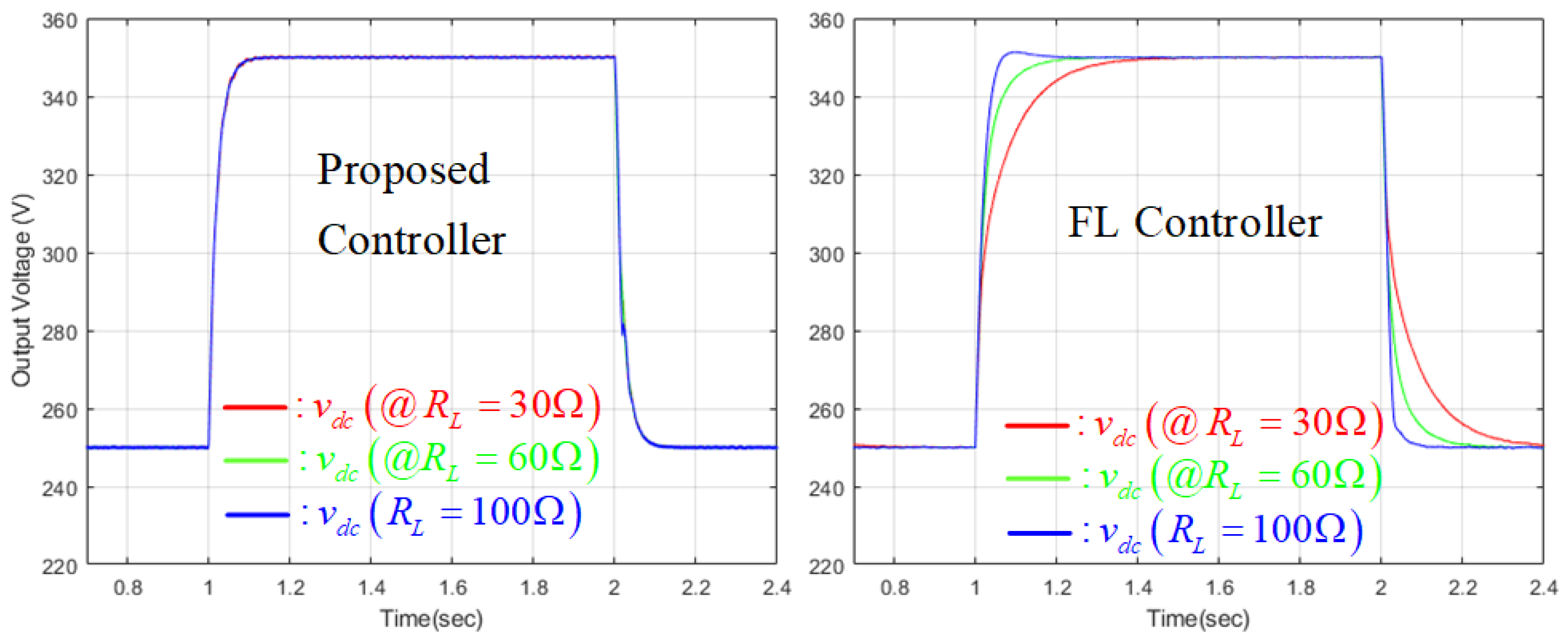
The first simulation evaluates the output voltage tracking performance for a time-varying output voltage reference that was increased from $v_{dc,ref}(t)=250\mathrm{V}$ to $v_{dc,ref}(t)=350\mathrm{V}$ and afterwards was restored to $v_{dc,ref}(t)=250\mathrm{V}$. This simulation was performed for three-types of resistive loads ($R_L=30,60,100\Omega$) to evaluate the closed-loop robustness against load variations. The resulting closed-loop output voltage behaviors are shown in Figure 5, and the trajectories of the estimated disturbances from the DOBs are depicted in Figure 6. Figure 7 shows the corresponding input DC voltage and PMSM speed responses that originated from the wind turbine and velocity. These results indicate that the proposed technique precisely assigned the desired output voltage tracking performance to the closed-loop system in the presence of model–plant mismatches and load variations, thanks to the DOBs.

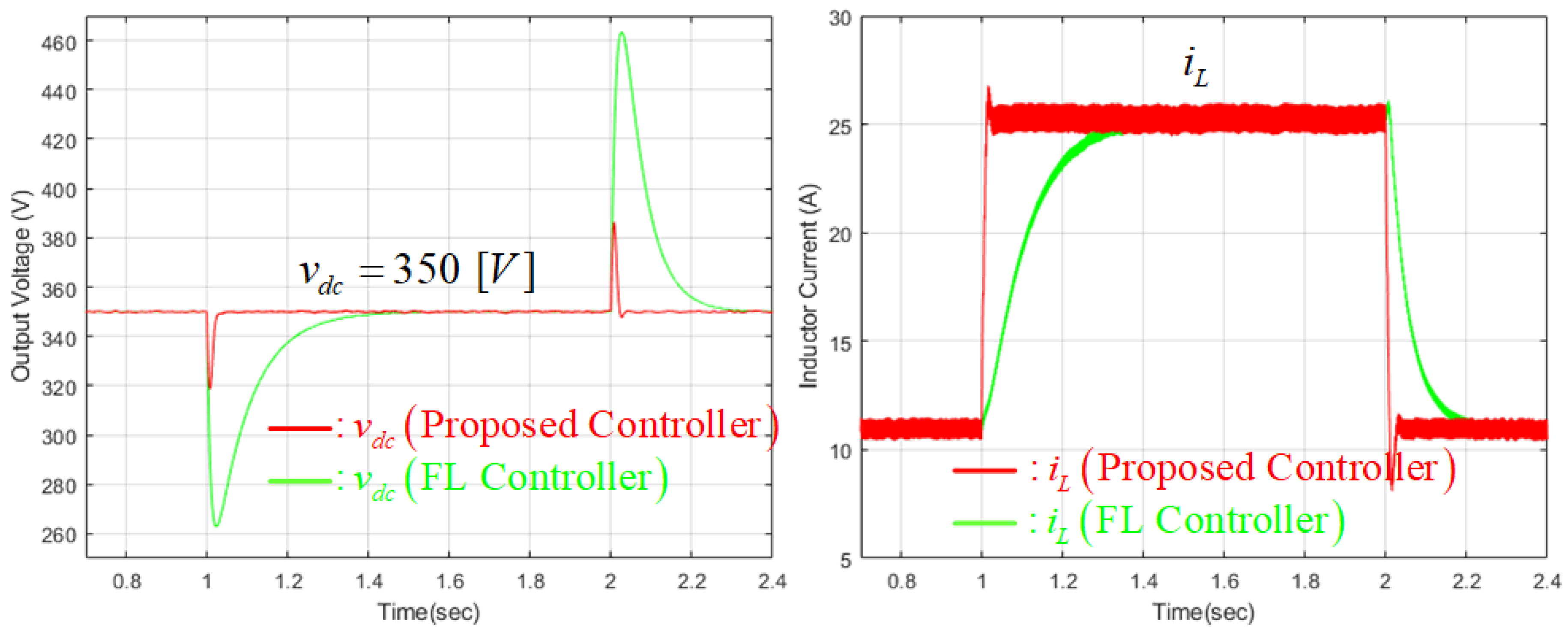
The second simulation investigates the output voltage regulation performance under a sudden load variation, where the resistive load of $R_L$ was changed from $R_L=60\Omega$ to $R_L=30\Omega$, and it was restored to $R_L=60\Omega$ in a sequential manner. The resulting closed-loop responses are depicted in Figure 8, which observes that the proposed technique considerably enhanced the output voltage regulation performance by speeding up the output voltage restoring rate with a rapid inductor current response. This feature was also obtained because the DOB exponentially estimated the disturbances coming from load current variations and model–plant mismatches.

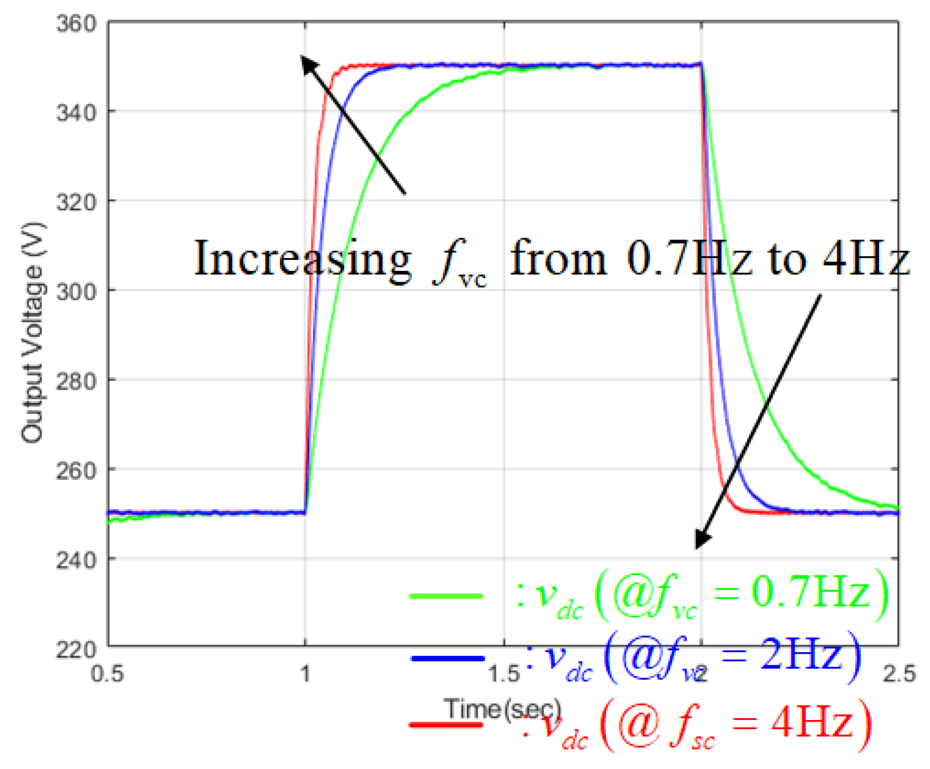
The last simulation examines the output voltage tracking performance change behaviors as increasing the cut-off frequency of $f_{vc}$ to $f_{vc}=0.7,2,4$ Hz. In this simulation, the output voltage reference was increased from $v_{dc,ref}(t)=250\mathrm{V}$ to $v_{dc,ref}(t)=350\mathrm{V}$ under a resistive load of $R_L=30\Omega$. The comparison results are presented in Figure 9, which indicates that the closed-loop output voltage tracking performance was precisely adjusted by the proposed technique using a fixed control parameter set in the presence of model–plant mismatches.

4.3. Discussion

These numerical verifications confirmed the beneficial closed-loop properties proven in Theorems 1 and 2, and this section clearly shows that a considerable output voltage tracking and regulation performance improvement can be obtained using the proposed technique in the presence of input voltage variations caused by wind speed changes. Therefore, it can be concluded that the proposed technique is qualified as a promising solution for wind power system applications.

5. Conclusions

For DC/DC boost converter applications, this paper suggests a passivity-based proportional-type output voltage tracking control algorithm incorporating the DOB under the PCH framework, which results in a classical cascade structure. The proposed control algorithm was derived by solving a PDE so that the closed-loop system had the desired positive-definite energy function. Moreover, it is shown that the proposed controller guarantees the performance recovery property by rendering the closed-loop energy function to be decreased exponentially, and it also ensures the offset-free property in the absence of tracking error integrators by analyzing the closed-loop steady-state equations. The beneficial closed-loop properties were numerically verified by emulating a wind power system equipped with a wind turbine, PMSM, three-phase diode rectifier, and DC/DC boost converter. In this study, the closed-loop cut-off frequency was manually found through a trial and error process, and it was fixed for all time. An auto-tuning mechanism for the closed-loop cut-off frequency will be devised and experimentally verified in a future study.

References

- Zhai, L.; Zhang, T.; Cao, Y.; Yang, S.; Kavuma, S.; Feng, H. Conducted EMI Prediction and Mitigation Strategy Based on Transfer Function for a High-Low Voltage DC-DC Converter in Electric Vehicle. Energies 2018, 11, 1028. [Google Scholar] [CrossRef]
- Tran, V.T.; Nguyen, M.K.; Choi, Y.O.; Cho, G.B. Switched-Capacitor-Based High Boost DC-DC Converter. Energies 2018, 11, 987. [Google Scholar] [CrossRef]
- Padmanaban, S.; Bhaskar, M.S.; Maroti, P.K.; Blaabjerg, F.; Fedak, V. An Original Transformer and Switched-Capacitor (T & SC)-Based Extension for DC-DC Boost Converter for High-Voltage/Low-Current Renewable Energy Applications: Hardware Implementation of a New T & SC Boost Converter. Energies 2018, 11, 783. [Google Scholar] [CrossRef]
- Park, Y.J.; Khan, Z.H.N.; Oh, S.J.; Jang, B.G.; Ahmad, N.; Khan, D.; Abbasizadeh, H.; Shah, S.A.A.; Pu, Y.G.; Hwang, K.C.; et al. Single Inductor-Multiple Output DPWM DC-DC Boost Converter with a High Efficiency and Small Area. Energies 2018, 11, 725. [Google Scholar] [CrossRef]
- Bi, H.; Wang, P.; Wang, Z. Common Grounded H-Type Bidirectional DC-DC Converter with a Wide Voltage Conversion Ratio for a Hybrid Energy Storage System. Energies 2018, 11, 349. [Google Scholar] [CrossRef]
- Zhang, S.; Wang, Y.; Chen, B.; Han, F.; Wang, Q. Studies on a Hybrid Full-Bridge/Half-Bridge Bidirectional CLTC Multi-Resonant DC-DC Converter with a Digital Synchronous Rectification Strategy. Energies 2018, 11, 227. [Google Scholar] [CrossRef]
- Erickson, R.W.; Maksimovic, D. Fundamentals of Power Electronics, 2nd ed.; Springer: New York, NY, USA, 2001. [Google Scholar]
- Alexander, G.P.; Feng, G.; Yan-Fei, L.; Paresh, C.S. A Design Method for PI-like Fuzzy Logic Controllers for DC/DC Converter. IEEE Trans. Ind. Electron. 2007, 54, 2688–2696. [Google Scholar]
- Olalla, C.; Leyva, R.; Queinnec, I.; Maksimovic, D. Robust Gain-Scheduled Control of Switched-Mode DC-DC Converters. IEEE Trans. Power Electron. 2012, 27, 3006–3019. [Google Scholar] [CrossRef]
- Su, J.T.; Liu, C.W. Gain scheduling control scheme for improved transient response of DC-DC converters. IET Power Electron. 2012, 5, 678–692. [Google Scholar] [CrossRef]
- Bibian, S.; Jin, H. High Performance Predictive Dead-Beat Digital Controller for DC Power Supplies. IEEE Trans. Power Electron. 2002, 17, 420–427. [Google Scholar] [CrossRef]
- Zhang, Q.; Min, R.; Tong, Q.; Zou, X.; Liu, Z.; Shen, A. Sensorless Predictive Current Controlled DC-DC Converter With a Self-Correction Differential Current Observer. IEEE. Trans. Ind. Electron. 2014, 61, 6747–6757. [Google Scholar] [CrossRef]
- Salimi, M. Sliding Mode Control of the DC-DC Fly back Converter with Zero Steady-State Error. J. Basic Appl. Sci. Res. 2012, 2, 10693–10705. [Google Scholar]
- Oucheriah, S.; Guo, L. PWM-Based Adaptive Sliding-Mode Control for Boost DC/DC Converters. IEEE Trans. Ind. Electron. 2013, 60, 3291–3294. [Google Scholar] [CrossRef]
- Linares-Flores, J.; Mendez, A.H.; G.-Rodriguez, C.; S.-Ramirez, H. Robust Nonlinear Adaptive Control of a Boost Converter via Algebraic Parameter Identification. IEEE Trans. Ind. Electron. 2014, 61, 4105–4114. [Google Scholar] [CrossRef]
- Kim, S.K.; Park, C.R.; Lee, Y.I. A Stabilizing Model Predictive Controller for Voltage Regulation of a DC/DC Boost Converter. IEEE Trans. Control Syst. Technol. 2014, 41, 2107–2114. [Google Scholar] [CrossRef]
- Kim, S.K.; Kim, J.S.; Park, C.R.; Lee, Y.I. Output-feedback model predictive controller for voltage regulation of a DC/DC converter. IET Control Theory Appl. 2013, 7, 1959–1968. [Google Scholar] [CrossRef]
- Beccuti, A.G.; Mariethoz, S.; Cliquennois, S.; Wang, S.; Morari, M. Explicit Model Predictive Control of DC/DC Switched-Mode Power Supplies With Extended Kalman Filtering. IEEE Trans. Ind. Electron. 2009, 56, 1864–1874. [Google Scholar] [CrossRef]
- Karamanakos, P.; Geyer, T.; Manias, S. Direct Voltage Control of DC-DC Boost Converters Using Enumeration-Based Model Predictive Control. IEEE Trans. Power Electron. 2014, 29, 968–978. [Google Scholar] [CrossRef]
- Wang, Y.X.; Yu, D.H.; Kim, Y.B. Robust Time-Delay Control for the DC/DC Boost Converter. IEEE Trans. Ind. Electron. 2014, 61, 4829–4837. [Google Scholar] [CrossRef]
- Wai, R.J.; Shih, L.C. Design of Voltage Tracking Control for DC-DC Boost Converter Via Total Sliding-Mode Technique. IEEE Trans. Ind. Electron. 2011, 58, 2502–2511. [Google Scholar] [CrossRef]
- Ortega, R.; van der Schaft, A.; Maschke, B.; Escobar, G. Interconnection and damping assignment passivity-based control of port-controlled Hamiltonian systems. Automatica 2002, 38, 585–596. [Google Scholar] [CrossRef] [Green Version]
- Mathew, S. Wind Energy: Fundamentals, Resource Analysis and Economics; Springer: New York, NY, USA, 2006. [Google Scholar]
Figure 1.
DC/DC boost converter topology.
Figure 2.
Wind speed pattern from Weibull distribution-based wind model.
Figure 3.
Wind power system configuration.
Figure 4.
Simulation parameter summary table.
Figure 5.
Output voltage tracking performance change behaviors for .
Figure 6.
Estimated disturbance behaviors.
Figure 7.
Permanent magnet synchronous machine (PMSM) speed and input voltage behaviors.
Figure 8.
Output voltage regulation performance comparison for sudden load change from to .
Figure 9.
Output voltage tracking performances for several cut-off frequencies, Hz.
© 2018 by the author. Licensee MDPI, Basel, Switzerland. This article is an open access article distributed under the terms and conditions of the Creative Commons Attribution (CC BY) license (http://creativecommons.org/licenses/by/4.0/).
Share and Cite
MDPI and ACS Style
Kim, S.-K. Passivity-Based Robust Output Voltage Tracking Control of DC/DC Boost Converter for Wind Power Systems. Energies 2018, 11, 1469. https://doi.org/10.3390/en11061469
AMA Style
Kim S-K. Passivity-Based Robust Output Voltage Tracking Control of DC/DC Boost Converter for Wind Power Systems. Energies. 2018; 11(6):1469. https://doi.org/10.3390/en11061469
Chicago/Turabian StyleKim, Seok-Kyoon. 2018. "Passivity-Based Robust Output Voltage Tracking Control of DC/DC Boost Converter for Wind Power Systems" Energies 11, no. 6: 1469. https://doi.org/10.3390/en11061469
Note that from the first issue of 2016, this journal uses article numbers instead of page numbers. See further details here.