Experimental Investigation of Static Stall Hysteresis and 3-Dimensional Flow Structures for an NREL S826 Wing Section of Finite Span

Abstract

Flow characteristics of an S826 airfoil at different Reynolds numbers, ranging from 40,000–400,000 (based on airfoil chord length) and angles of attack from −10–25 degrees are thoroughly investigated in a low-speed wind tunnel. The airfoil’s lift and drag polars are first measured, and with a focus on pitching the airfoil in upstroke and downstroke orders, static stall hysteresis is identified in selected experiments at Reynolds numbers below 100,000 near the stall angle and subsequently investigated. Experiments using wire-generated free stream turbulence are conducted, and the hysteresis effects are shown to disappear when introducing a free stream turbulence of less than 2.5%. Further, spanwise flow is detected by comparing lift and drag values measured using both surface pressure integration at one cross section as well as integral force gauge measurement, and the surface oil flow visualization technique is subsequently used to study the 3D flow topologies formed on the airfoil. The formation of distinct stall cells on the suction side of the airfoil is observed at Reynolds numbers above 100,000 near the stall angle. By repeating the experiments, stall cells are proven to be reproduceable, although the identical geometries are necessarily not retained in abscence of surface impurities such as tapes. The effect of disturbances on the stall cells is investigated by utilizing roughness elements on the airfoil surface, and it is found that while such disturbances tend to change the shape of the stall cells, they do not contribute to the creation, nor destruction of the cells. Polar and visualisation measurements are also used to study flow separation, and it is observed that the separation location, as well as the laminar separation bubble, moves towards the leading edge when increasing the angle of attack.

1. Introduction

The aerodynamics at low Reynolds numbers is of high relevance for the design of small domestic wind turbines with rotor diameters ranging from 2–7 m, corresponding to rated generator capacities of 0.3–10 kW. Laboratory-scale rotors and wind turbines used for research purposes (e.g., [1,2,3]) are other examples of such flow regimes, while the flight of insects and unmanned aerial vehicles (UAV) are among the more general applications. UAVs are remotely-controlled small aerial vehicles operating at low chord Reynolds numbers (between 10,000 and 500,000; see [4]). They are used as play toys in the entertainment industry and as tools for topography inspection. Other examples of low Reynolds number flows include flows in turbo-machinery blades and micro-air-vehicles [5]. Transitional Reynolds number flows around airfoils are complex in nature and may lead to uncertainties in the aerodynamic performance. In order to maximize the efficiency, it is essential to understand the physics of flows over airfoils at low Reynolds numbers.

Airfoils and lifting surfaces at low Reynolds numbers are often prone to exhibiting a somewhat challenging behavior owing to the laminar-turbulent transition and separation of the flow, which makes it difficult to understand the flow features entirely. Where the flow on the suction side of the airfoil is subject to an adverse pressure gradient, the boundary layer undergoes a transition to turbulence by the magnification of fluctuations and generation of unsteady vortex structures, followed by flow separation. This process is referred to as separation-induced transition [5]. The turbulent flow then re-attaches to the surface and forms a separation bubble (SB). The highly energetic turbulent boundary layer keeps attached to the surface and withstands the adverse pressure gradients some distance downstream until the final possible turbulent separation appears at high angles of attack (see [4,6,7,8,9]).

The separation bubble is insignificant when the chordwise extent of the airfoil is smaller than 1% (short SB), especially on thin airfoil sections near the leading edge where large pressure gradients exist [10]. The short SBs can burst and lead to long SBs when increasing the angle of attack or when decreasing the Reynolds number [11] with the SB spanning a considerable part of the chord. Long SBs are usually seen on thick airfoils at low Reynolds numbers, as discussed in [5], and can significantly impact the aerodynamic behavior of airfoils.

Lifting surfaces, such as wings or wind turbine blades, are often designed using two-dimensional airfoil polars, utilizing a blade element approach assuming little or no mutual influence between the spanwise-located elements. However, the 2D flow on a rectangular wing produces 3D “mushroom” structures known as stall cells at high angles of attack due to the periodic spanwise breakdown of vortices that are created on the airfoil suction side [12,13]. This contradicts the assumption of local two-dimensionality of the flow. It is also known that the number of vortex pairs increases with the aspect ratio (span-to-chord ratio) (see [12]) and that the number and location of stall cells can be different at two different realizations of the same flow condition [14,15].

Due to the impact of such large flow structures on the separation location, understanding the mechanisms through which stall cells are generated and formed is of crucial importance. The work by Boiko (1996) [16] contains a detailed qualitative comparison of various findings of the formation of stall cells. Quantitatively, stall cells have been identified using experimental techniques such as tuft visualization [14,17,18], particle image velocimetry (PIV) [17,19] and surface flow visualization [12,19]. Due to their intrinsic beauty and physical significance, stall cells have been subject to theoretical and numerical analyses; see, e.g., [13,20,21]. Broeren et al. (2001) [18] have shown that the formation of stall cells is related to the separation from the trailing edge, unlike the laminar separation bubble (which is usually near the leading edge). In a recent research work, the effects of the aspect ratio on the formation and characteristics of the stall cells were investigated by [22] using a series of Reynolds-Averaged Navier-Stokes (RANS) and Delayed-Detached Eddy Simulation (DDES) numerical simulations on the symmetric NACA0012 airfoil. They found deterioration of aerodynamics (lift drop and increase in drag) associated with the formation of stall cells. They also found that the stall cells appear to have spacings around 1.4- and 1.8-times the chord length. The extent of spanwise spacings of stall cells agrees well with other numerical simulations performed on the S826 airfoil [23], suggesting a possible independence of the stall cell from the airfoil geometry.

Recent wind turbine rotor experiments and CFD investigations [2,24] have suggested that the airfoil investigated in the current study exhibits a complex flow behavior at the operating Reynolds numbers in the range from 40,000–200,000. In order to understand the flow physics with respect to this specific airfoil, we performed a series of numerical and experimental studies [23,25] to provide accurate tabulated airfoil data as input to the computational tools such as blade element momentum (BEM) codes and actuator line/disc models. A few articles have recently been published to investigate some aspects of the S826 airfoil [23,25,26,27]. However, these investigations are limited to some few specific cases and do not go into detail of other complexities such as static stall hysteresis and stall cell formation. This article is an extension of an earlier work ([28]) and aims at presenting more details of wind tunnel measurements in order to provide a deeper understanding of the fluid flow phenomena and the mechanisms in which stall cells are formed. With this in mind, the structure of this article is as follows: after the current introduction, Section 2 presents the airfoil geometry, as well as experimental setup. Details of lift, drag and pressure measurements, investigation of stall hysteresis, as well as oil flow visualization are covered in Section 3, and conclusions from various experiments are drawn in Section 4. The airfoil data for a wide range of Reynolds numbers and angle of attack are appended at the end for possible future validation studies.

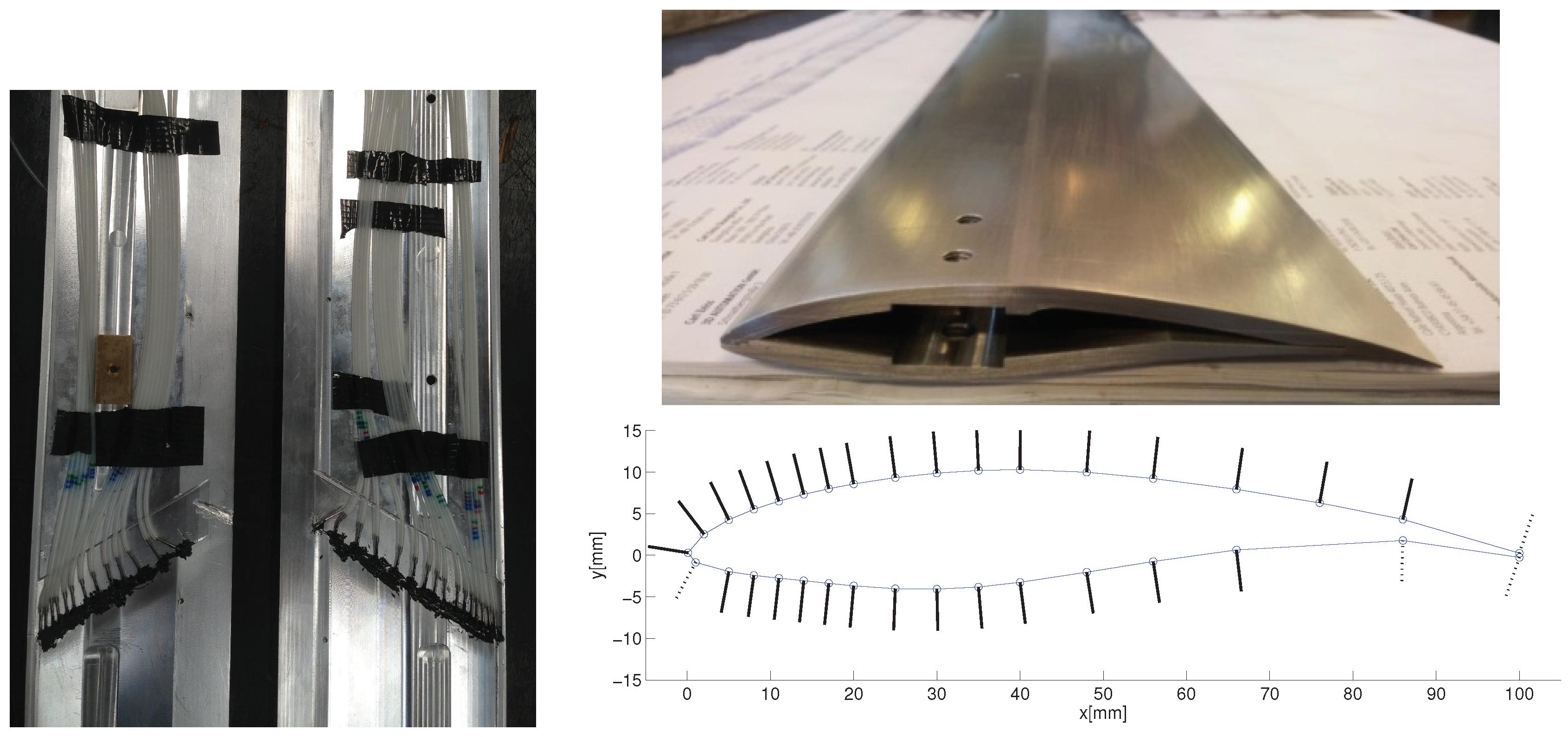
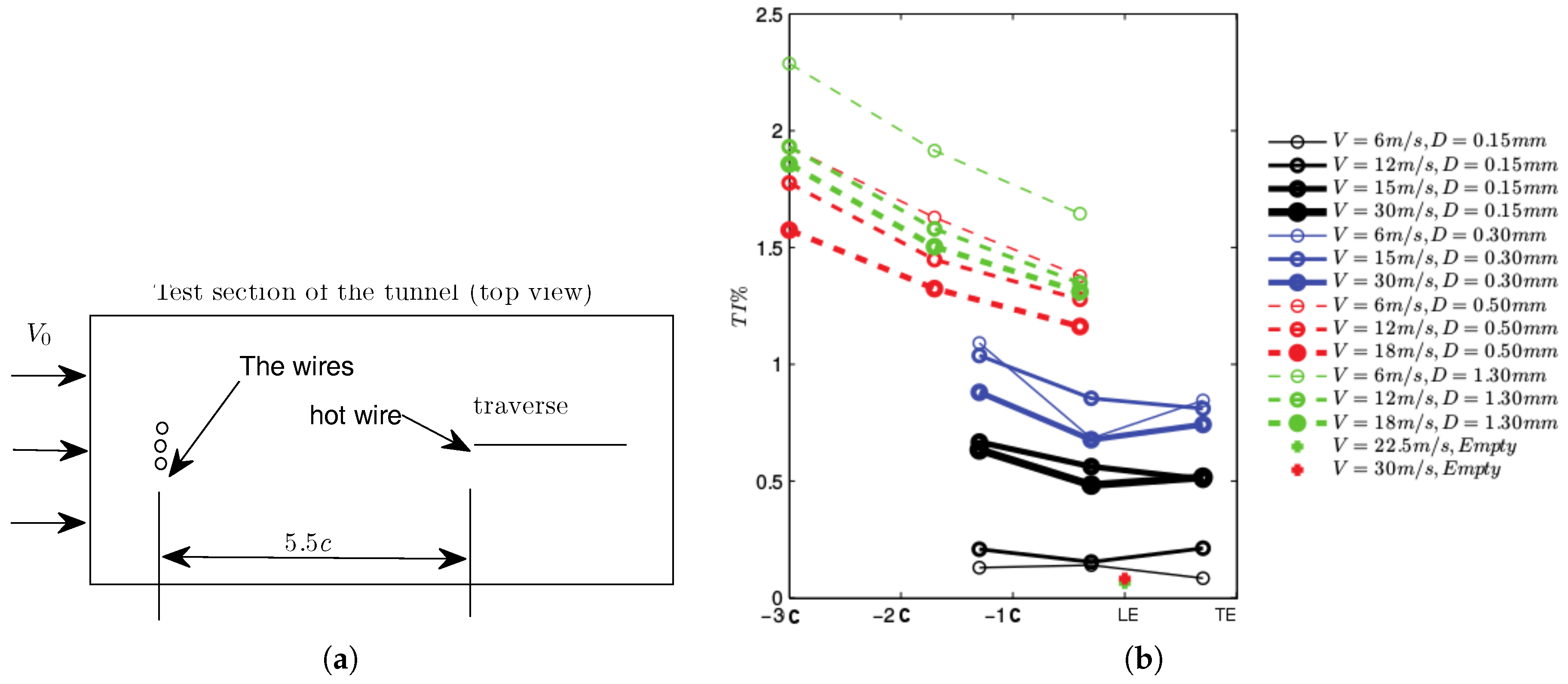
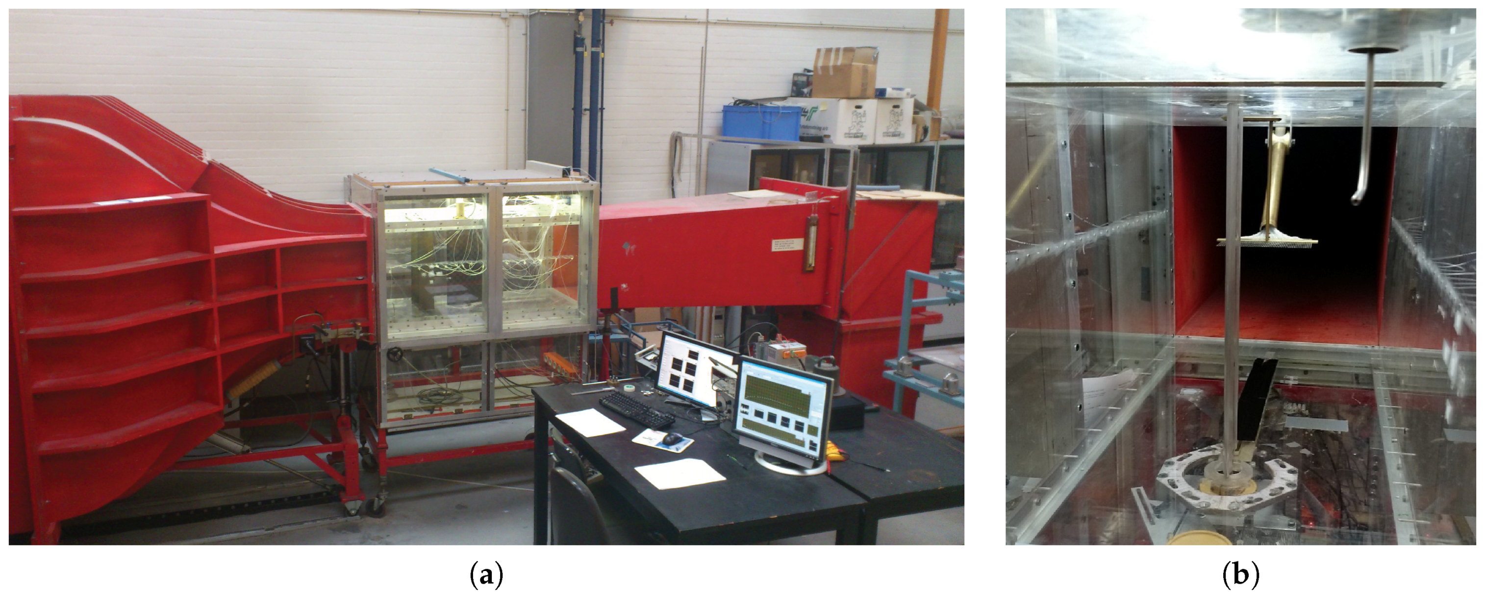
2. The Experimental Setup

The experiments were performed in a low-speed open-loop wind tunnel as shown in Figure 1a. The tunnel’s test section measures 1.3 m × 0.5 m × 0.5 m in streamwise, lateral and vertical directions, respectively, and due to a contraction ratio of 1:12.5, it is capable of delivering a uniform maximum velocity of $U_{\infty }$ = 65 m/s with a maximum turbulent intensity of about $0.1\%$ [28]. The vertically-mounted S826 airfoil shown in Figure 1b measures 100 mm in chord and 499 mm in span, leaving 0.5 mm of clearance between the airfoil and the side walls of the tunnel to minimize wall effects.

The wind tunnel is equipped with a one component, full bridge force balance for lift measurements, a wake-rake for wake and subsequently drag measurement (the latter being based on analysis of momentum loss and valid at pre-stall attached flow) and multiple pressure taps on sidewalls of the test section, which can be used to investigate flow uniformity, as well as lift integration. The bottom of the airfoil is connected to the force gage through a connection rod where the other end can rotate freely. Two different gages with $\pm 200$ N ($\pm 0.03$ N) and $\pm 20$ N ($\pm 0.002$ N) are used depending on the magnitude of forces experienced by the wind. The wake-rake, consisting of 32 measuring points, is mounted $x=1.6c$ downstream of the airfoil and at a height $z=2.1c$ of the test object. Airfoil pitching is performed using a set of JVL MAC servomotor with a resolution of 4096 pulses per revoluttion and encoder with an accuracy of $\pm 0.01°$. Thirty pressure taps are mounted unevenly over the airfoil at mid-span and along a 30${}^{\circ }$ chordwise line. A static pitot tube is installed at the inlet section of the wind tunnel to measure the reference pressure and subsequently the free-stream velocity. Pressure measurements for the airfoil surface and tunnel walls are performed using two sets of PSI pressure scanners with pressure ranges of $\pm 6895$ Pa ($\pm 1$ psi) and $\pm 2540$ Pa (±10 in H${}_2$O) and a sampling frequency of 125Hz for a duration of 10 seconds at each angle of incidence in the upstroke (from −10${}^{\circ }$ to 25${}^{\circ }$), as well as in the downstroke (+25${}^{\circ }$–−10${}^{\circ }$) pitching (For experiments at Re> 200,000, the more sensitive sensor is mounted on the walls as opposed to the airfoil surface to experience lower peak pressures, and vice versa). The first and last one-second of acquired data for each angle of attack are excluded for post-processing to avoid transitional effects, therefore a total of 1000 useable realizations for each experiment is analysed. The wake-rake and sidewall pressure taps are connected to the same pressure sensors as those used for the airfoil. The stagnation pressure is then measured in front of each tube. The airfoil is made of aluminum using Computer Numerical Control (CNC) milling, with a surface accuracy of $\pm 0.01$ mm. Due to the machining limitations, the trailing edge is cut with a finite thickness of $0.5$ mm. Figure 2 shows the location of the pressure taps and the corresponding normal vectors at each location.

3. Results and Discussions

3.1. Wind Tunnel Measurement

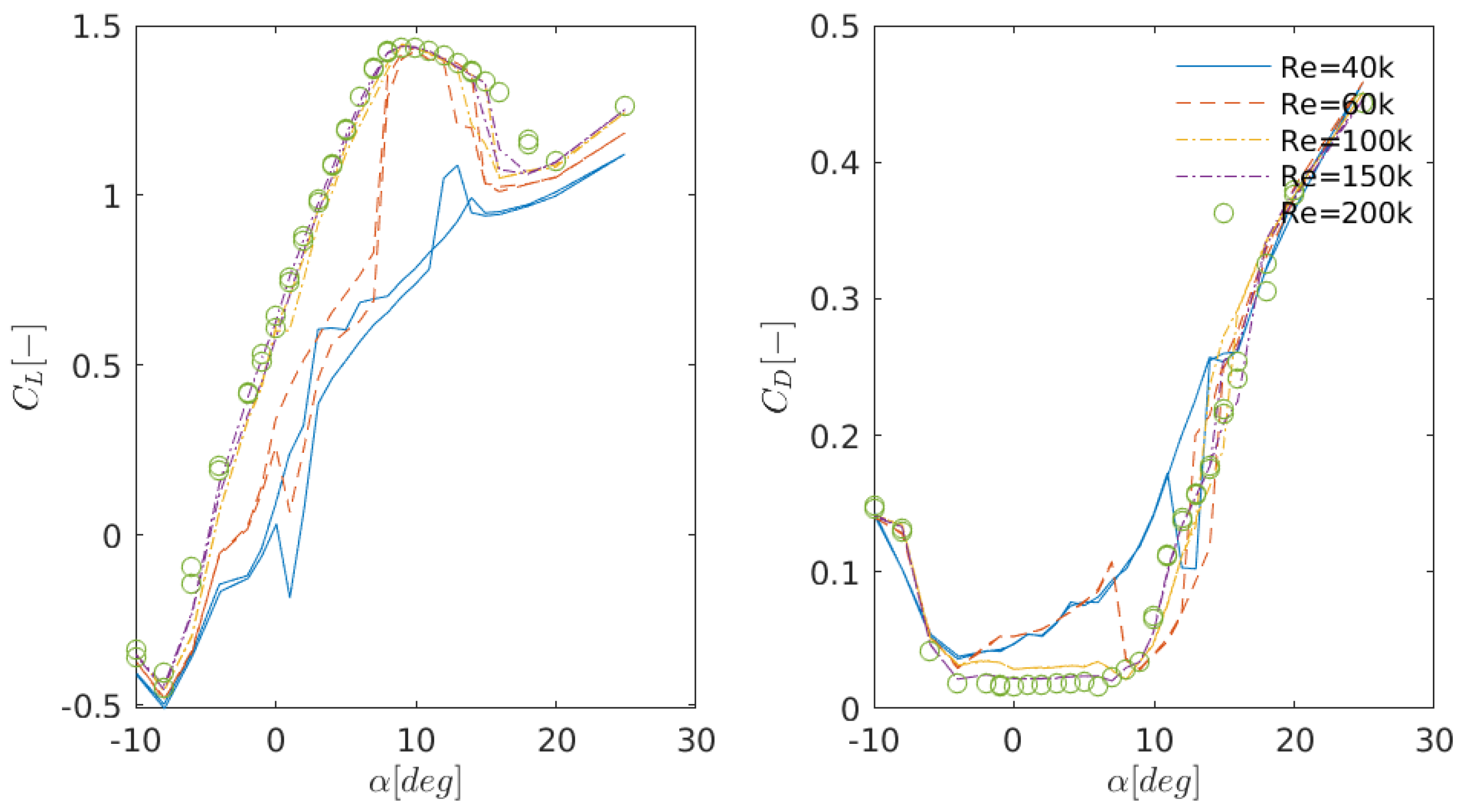
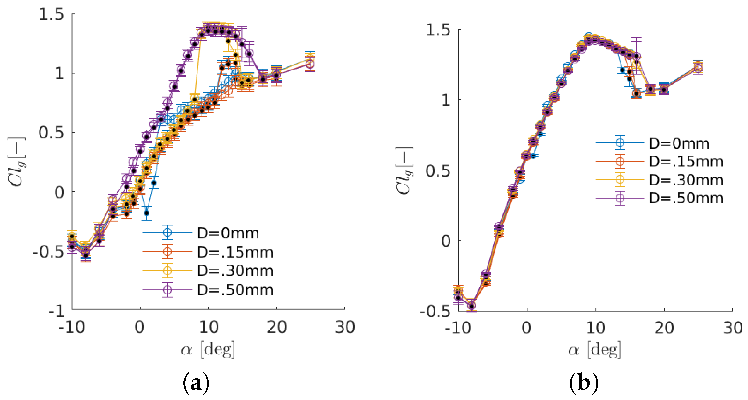
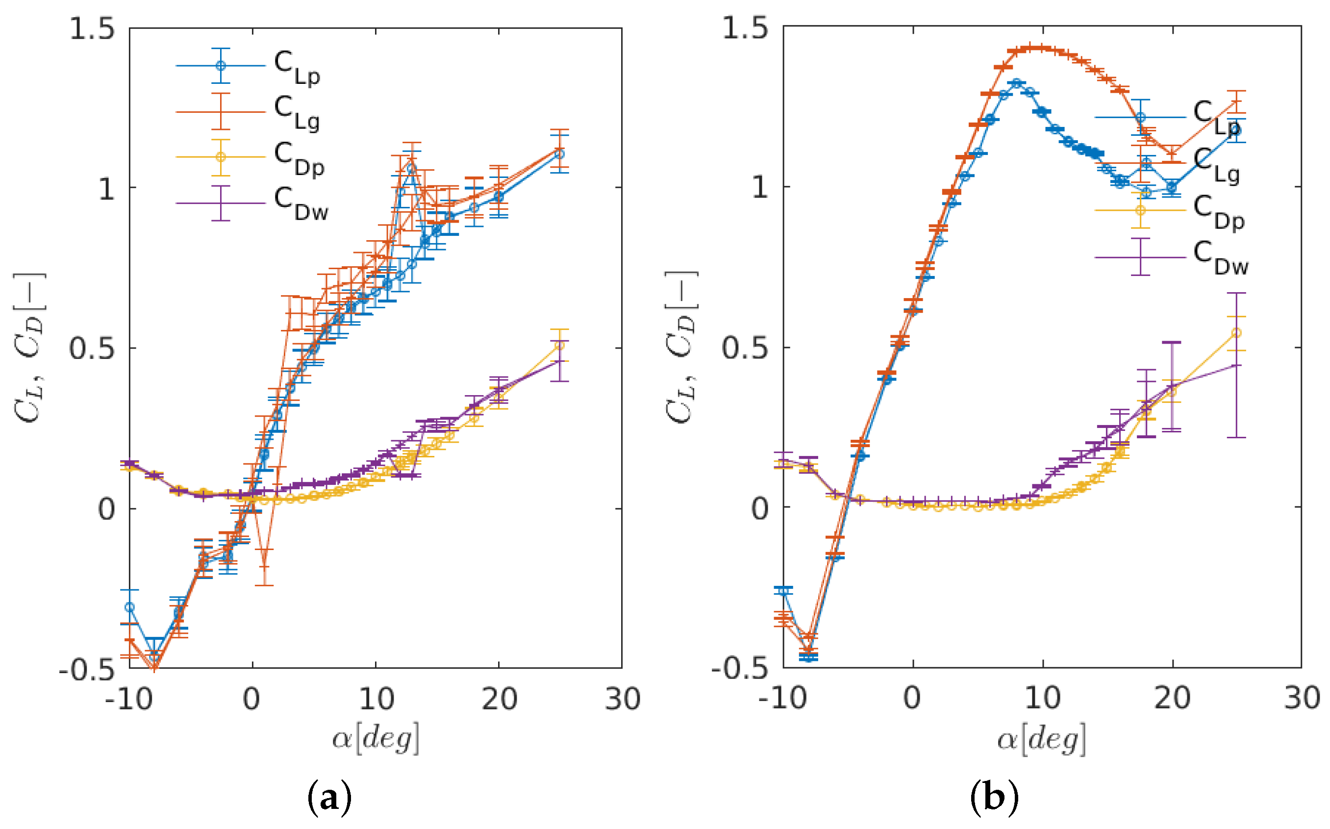
3.1.1. Polar Measurements

Figure 3 shows the lift and drag polars at different Reynolds numbers. As can be observed from the figure and the appendices, there is a very small difference between the lift coefficients at Reynolds numbers above 100,000 at the post-stall angles. It can also be seen that the lift and drag coefficients corresponding to Re = 40,000 result in different values for increasing (upstroke) and decreasing (downstroke) the angle of attack. This is due to so-called static stall hysteresis (the ability of flow to remember its past history). Static stall hysteresis will be thoroughly discussed in Section 3.1.4. Note that the error bars indicating uncertainties in the measurements are omitted in this figure for more clarity, but are discussed in the next sections.

3.1.2. Wind Tunnel Correction

The presence of the wind-tunnel walls has an impact on the airfoil measurements in the form of an increase in the measured lift, drag and pitching moments, due to the velocity increase around the model. The lateral walls in a 2D airfoil measurement cause solid blockage, wake blockage and streamline curvature effects, as investigated. The measured polars in this research are corrected against correction procedures proposed by [29,30], and the lift-drag ratios are plotted in Figure 4. As can be seen, the effect of tunnel correction is negligible as the test section-to-airfoil area ratio is adequately large.

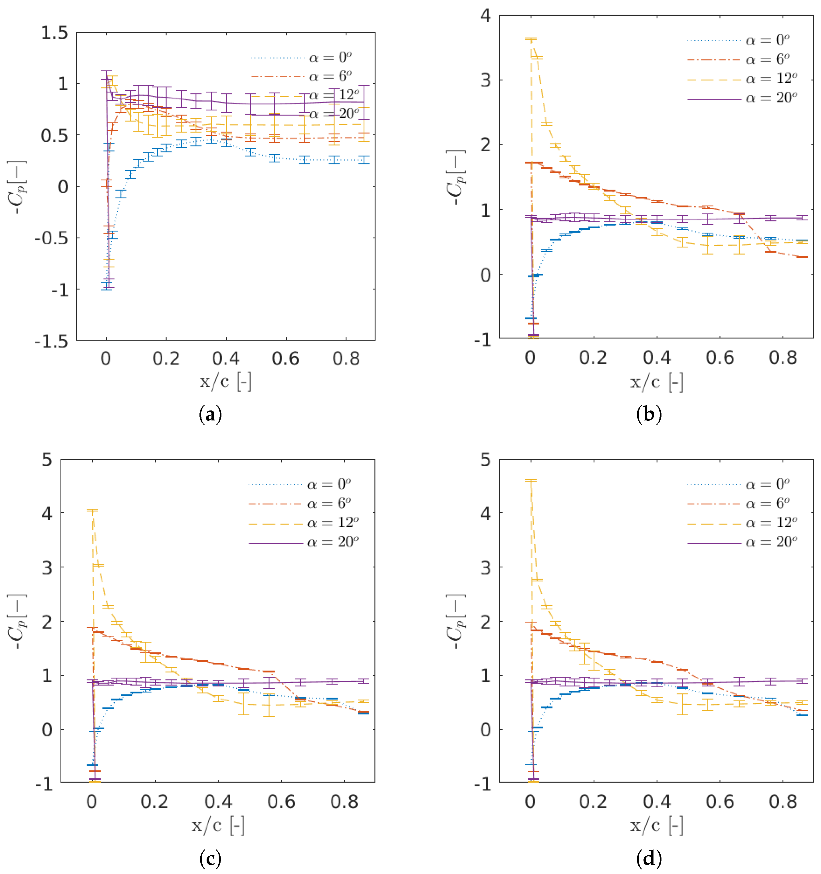
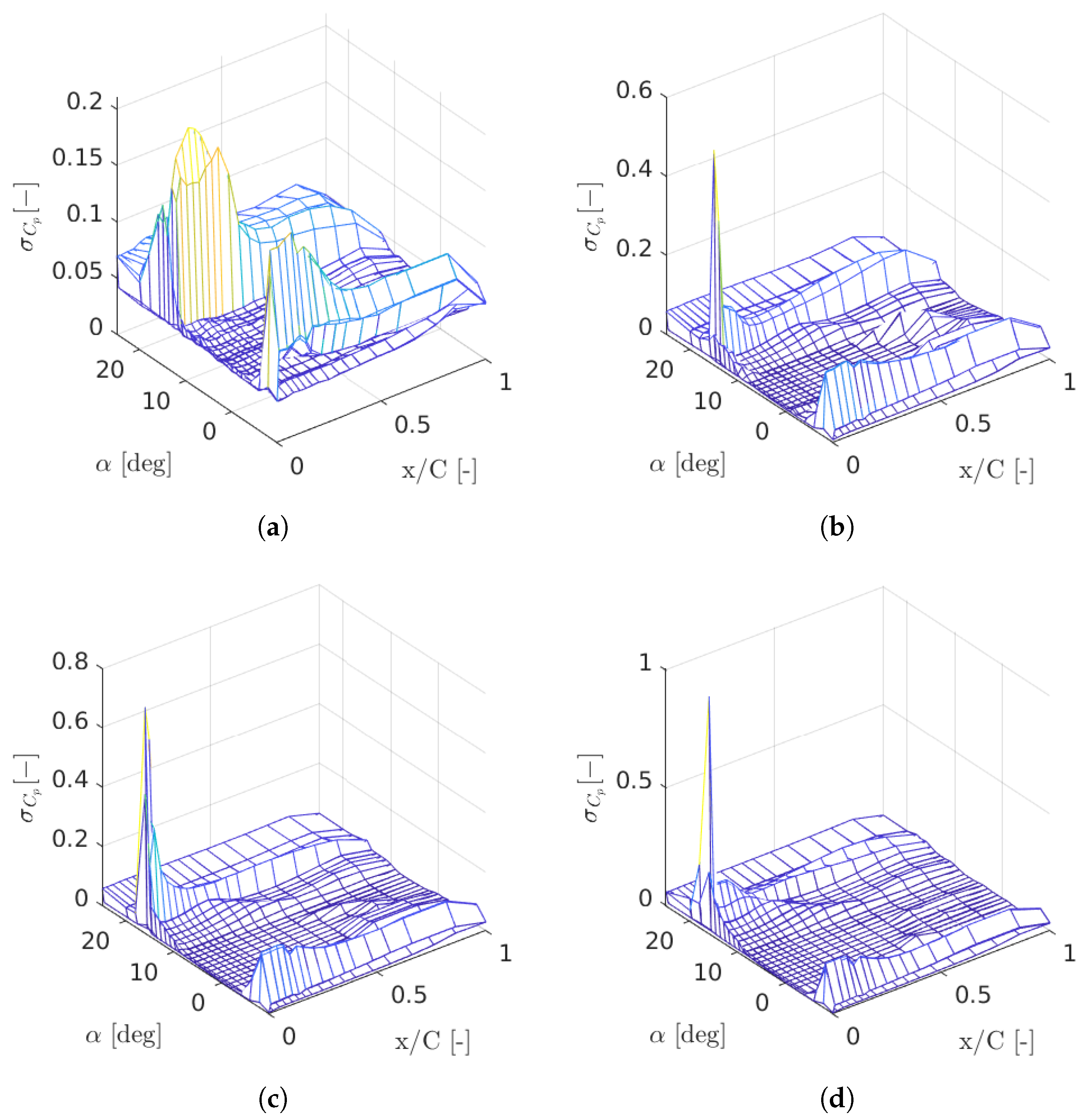
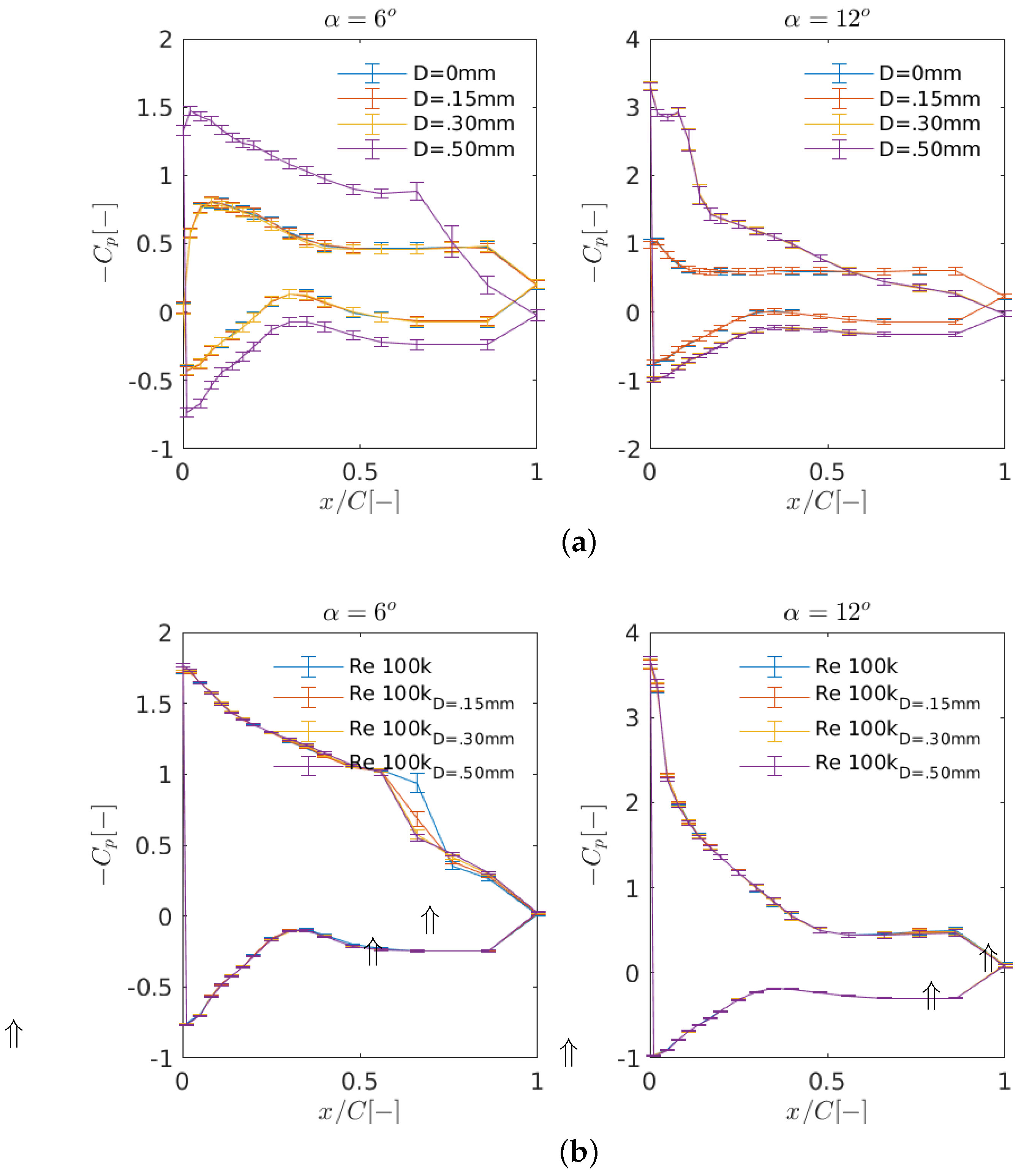
3.1.3. Pressure Distribution

Figure 5 represents the pressure coefficient on the suction side of the airfoil for various free stream velocities, $V_{\infty }$. Here, the pressure coefficient is calculated as:

$$C_p=\frac{p_i-p_{\infty }}{\frac{1}{2}{\rho }_{\infty }{V}_{\infty }^2}$$

(1)

where ${\rho }_{\infty }$ is the freestream density, $p_i$ is the static pressure at the i-th pressure tap, $p_{\infty }$ is the static pressure in the free stream and the denominator is the dynamic pressure calculated as $p_0-p_{\infty }$ with $p_0$ being the stagnation pressure in the freestream. Each figure contains four curves corresponding to different measured angles of attack. The standard deviation of the measured signal is also plotted on top of the pressure measurement for all cases, and for clarity, only the pressure distributions on the suction side of the airfoil are shown in the figures (pressure side values do not represent any significant phenomena). As expected, the suction peak becomes larger with increasing Reynolds numbers, especially at AoA = 12${}^{\circ }$. From Figure 5a, the pressure increases with the angle of attack until the stall angle. The suction peak also gets larger with the angle of attack. In some cases, a pressure plateau is observed, indicating a laminar separation bubble. From the standard deviations, it is clear that the variability of measurements is substantially higher at Re = 40,000, which is due to higher unsteadiness associated with the flow.

Uncertainties associated with the experiments are also quantified. In comparison with temperature and density variations and other instrument uncertainties, local flow variability due to wind tunnel turbulence and blockage effects especially at higher angles of attack are found to be the main contributors to the uncertainties. Figure 6 shows the standard deviation at each pressure tap and for each angle of attack for various Reynolds numbers. It is found that the peak of the standard deviation occurs near the leading edge and around stall angles. Cases at Re = 40,000 generally exhibit higher uncertainties, especially near mid-chord, which is a result of flow unsteadiness in such cases.

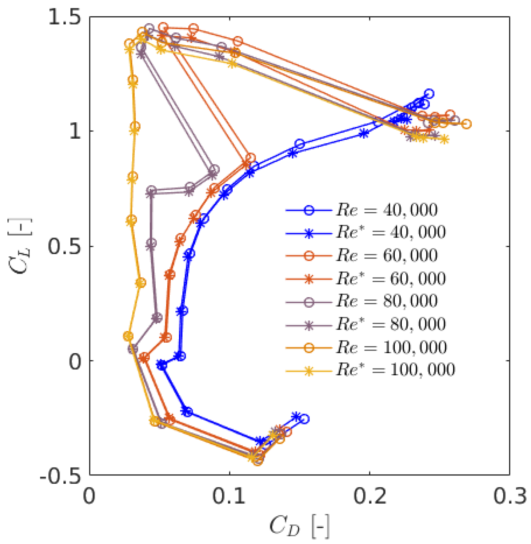
3.1.4. Stall Hysteresis

At low Reynolds numbers, the turbulent momentum transport is smaller than the adverse pressure gradient effect; hence, the momentum flux is not able to close the bubble, and a large separation bubble, potentially up to the trailing edge, is formed. This is followed by a further increase in $C_D$ and a loss of $C_L$, resulting in a nonlinear behavior in the lift and drag prediction and a strong hysteresis effect. This effect can be discarded by triggering turbulence near the leading edge (LE) of the airfoil. To investigate the sensitivity of the airfoil to the hysteresis behavior at low Reynolds numbers, an experiment has been performed by locating a set of three parallel wires with cylindrical cross-sections vertically at a distance of $5.5c$ upstream of the test section to produce a turbulent in-flow with a small amount of turbulence intensity. To get an accurate measure of the turbulence levels produced by the wires, they are put in the empty test section, and the turbulence intensity produced by the wires is measured using a single sensor (5-$\mathsf{\mu }$m tungsten wire) hot-wire probe, moving on a 1D traversing system. Figure 7a shows a sketch of the wire configuration used to generate turbulence, and Figure 7b shows the corresponding turbulence intensities at different locations downstream of the test section giving the decay of turbulence alongside the tunnel. The empty tunnel without wires is represented by the markers for $U_{\infty }=22.5$ and 30 m/s, and four wires of 1.3 mm, 0.5 mm, 0.3 mm and 0.15 mm in thickness are used for the investigations. To get an idea of what type of disturbance we are creating using each wire configuration, a simple calculation of the Reynolds numbers is carried out and presented in

Table 1. Approximate Reynolds numbers associated with various wires tested in the wind tunnel.

U [m/s]	${\mathit{\sigma }}_{\overline{\mathit{U}}}$	Re${}_{\mathit{airfoil}}$	Re${}_{\mathit{wire}}$
			D = 0.15 mm	D = 0.3 mm	D = 0.5 mm	D = 1.3 mm
6	0.0057	40,000	60	120	200	520
15	0.0054	100,000	150	300	500	1300
30	0.0063	200,000	300	600	1000	2600

. In the table, ${\sigma }_{\overline{U}}$ corresponds to the standard deviation of the empty wind tunnel velocity, averaged over all measured angles of attack. As seen in the table, the lowest and highest Reynolds numbers based on wire diameter are 60 and 2600 for U = 6 m/s (chord-based Reynolds number of Re = 40,000) and U = 30 m/s (chord-based Reynolds number of Re = 200,000). This corresponds to a range of flow regimes with laminar vortex shedding up to turbulent vortex streets. As it is not our intention to further examine flow around a cylinder, we refer the interested reader to other references (e.g., [31]) to gain further insight into flow physics at such Reynolds numbers. For brevity, the other Reynolds numbers are not shown here.

The turbulence intensities are measured at different downstream locations where a decay of turbulence can be seen for almost all cases. Thicker wires produce higher turbulence as they correspond to a higher wire Reynolds number. On the other hand, the turbulence levels are generally higher at lower velocities due to the quality of the wind in the wind tunnel. Here, we use the results shown in Figure 7a as an indication of the free stream turbulence generated by each wire at the corresponding wind velocity in the tunnel (chord Reynolds number). For example, the 1.3 mm-thick wire setup produces turbulence intensities of $2.28\%$, $1.93\%$ and $1.85\%$ at wind speeds of 6 m/s (Re = 40,000), 12 m/s and 18 m/s at three chords upstream of the airfoil LE location ($\frac{x}{c}=-3$). The turbulence then decays as particles get closer to the airfoil. At a wind velocity of 6 m/s (Re = 40,000), the wire setups of 0.15, 0.30 and 0.5 mm in thickness produce an added turbulence of 0.14, 0.68 and 1.37%, respectively. These will be used to quantify the aerodynamics of the S826 airfoil in the following.

As a first visual assessment of the effect of added turbulence at Re = 40,000, flow structures in the wake of the airfoil are compared, and the wave velocity time series at certain angles of attack and at the center of the wake rake ($\gamma /c=0$), as well as average wake velocities behind the airfoil are shown in Figure 8. Two cases are considered for comparison: the least turbulent case without wire-generated turbulence (D = 0 mm) and the case with the highest wire-generated turbulence among considered experiments (D = 0.50 mm). It is generally clear that, following the previous literature, adding the extra turbulence enhances flow attachment, thereby reducing the fluctuating signals. This effect is more pronounced at $\alpha =6^{\circ }$ and $\alpha ={12}^{\circ }$, where a significant reduction of fluctuations and a smaller wake are seen by adding turbulence to the flow. A lower drag is therefore expected for the extra turbulence case due to smaller wake velocities. At $\alpha =0^{\circ }$ and $\alpha ={20}^{\circ }$, the flow is fully attached and fully separated, respectively. Therefore, no significant impacts of adding the turbulence are seen.

Figure 9 and Figure 10 show the effect of the free-stream turbulence on lift and pressure measurements at Re = 40,000 and Re = 100,000. The impact of inflow turbulence on the temporal variability of the pressure measurements is also examined through plotting the error bars shown in both figures. At low Reynolds numbers, the use of wires results in a higher pressure distribution, which leads to higher lift coefficients. At $\alpha ={12}^{\circ }$, the two wires of thickness D = 0.30 mm and D = 0.50 mm reach an asymptotic behavior, which means no further changes will occur in the aerodynamics for higher turbulence levels. However, at Re = 100,000, results obtained using different turbulence levels are very similar as the hysteresis is almost disappearing at such higher Reynolds numbers. At $\alpha ={12}^{\circ }$, no change can be observed in the aerodynamic values, and for $\alpha =6^{\circ }$, adding turbulence results in a slightly smaller separation jump close to the trailing edge (TE). From the lift polars for Re = 40,000, mounting a wire of D = 0.50 mm at the inlet removes the hysteresis almost completely and results in a rise in the lift curve. The increase in turbulence intensity, therefore, has a similar impact on the airfoil performance as the increase in Reynolds number. The general trend of an inverse relation between hysteresis and free stream turbulence agrees well with the literature (see e.g., [32]).

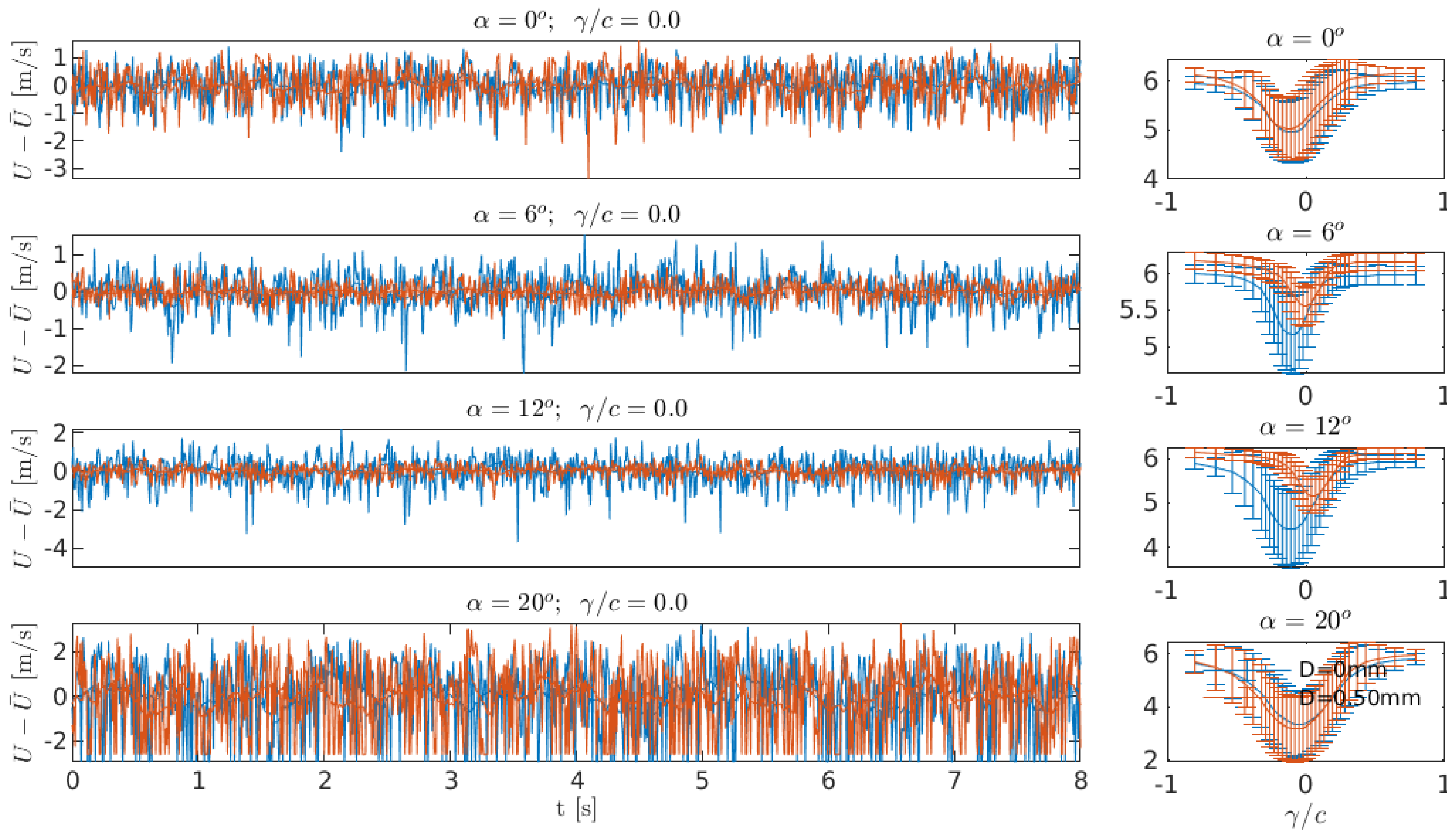
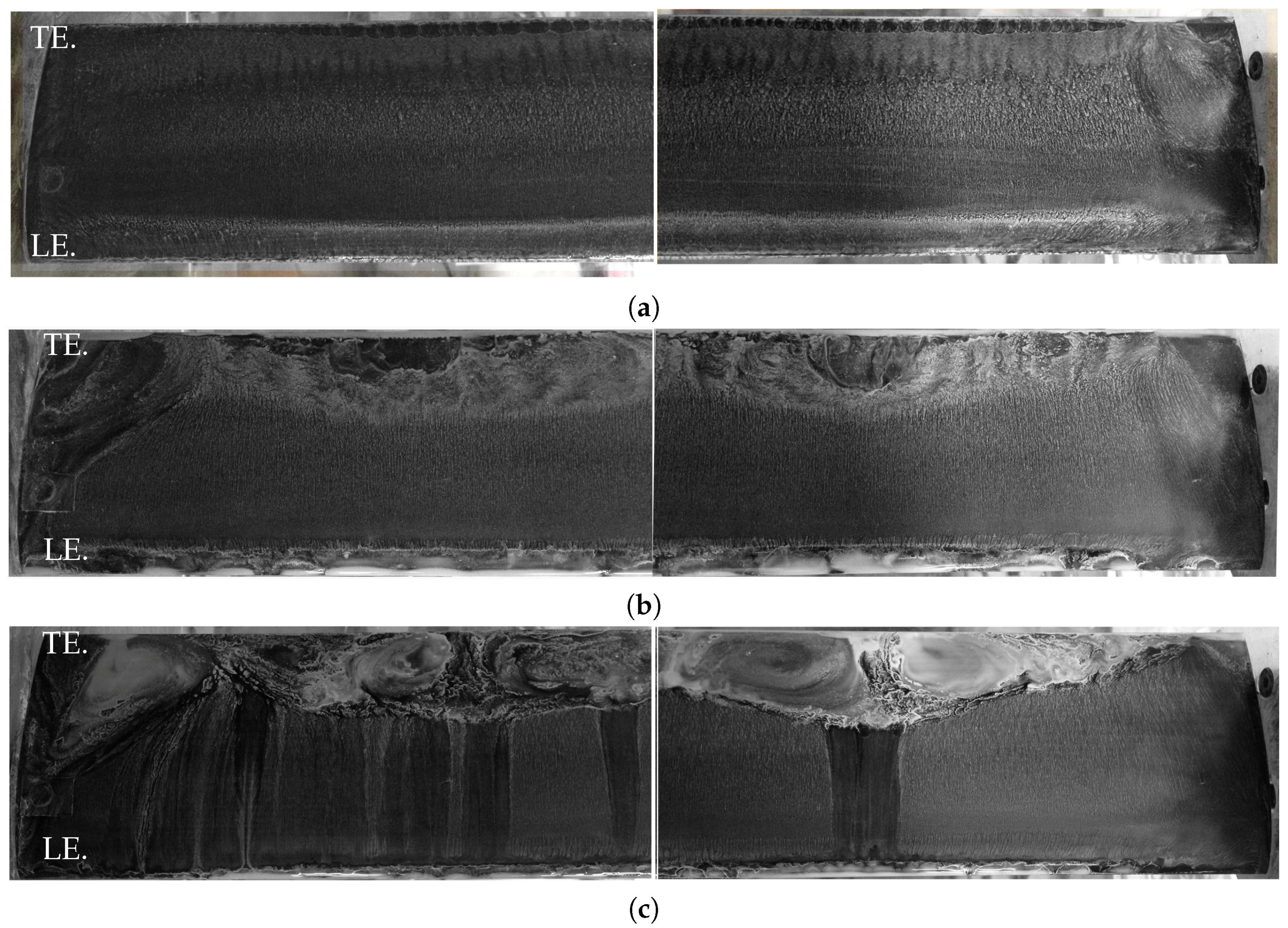
3.2. Identification of Three-Dimensional Flow over the Airfoil

In this paper, lift coefficients have been measured using both integration of surface pressure ($C{l}_p$) and through direct reading of the force gauge ($C{l}_g$). As presented earlier, pressure measurements have only been performed over an inclined line of pressure taps and not through the entire span; therefore, assuming an adequate number of pressure tap readings, which is to a high degree the case in current experiments, a nonidentical lift value given by gauge and pressure measurements is a direct indication of the three-dimensionality of the flow over the airfoil. A similar argument can be made for drag measurements using surface pressure integration ($C{d}_p$), as well as momentum analysis using wake rake pressure scanners ($C{d}_w$), which happens at a spanwise location other than airfoil pressure taps. Figure 11 shows such a comparison of lift measurements for Reynolds numbers 40,000 and 200,000. As can be seen, for both cases, there is an inconsistency between both measurements, which reveals the presence of 3D effects. Further analysis of spanwise flow structures is presented in the following section.

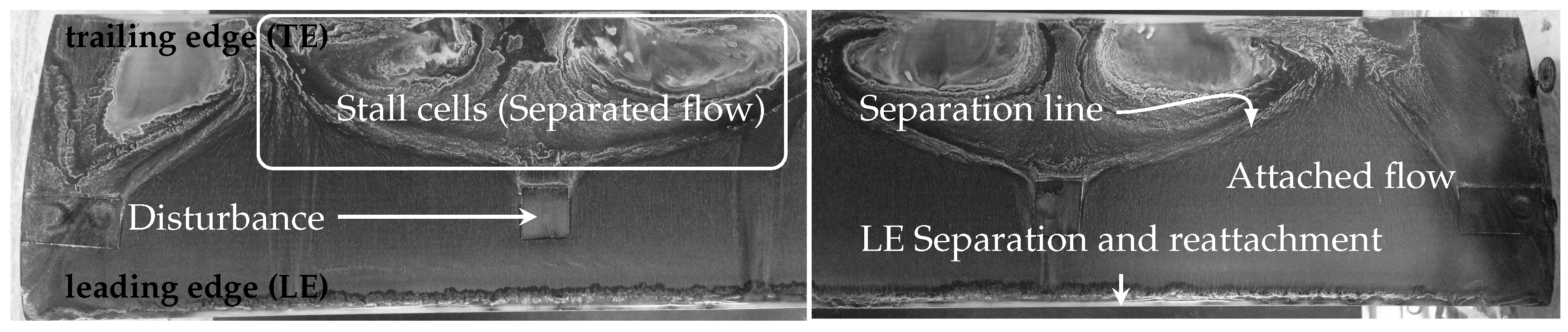
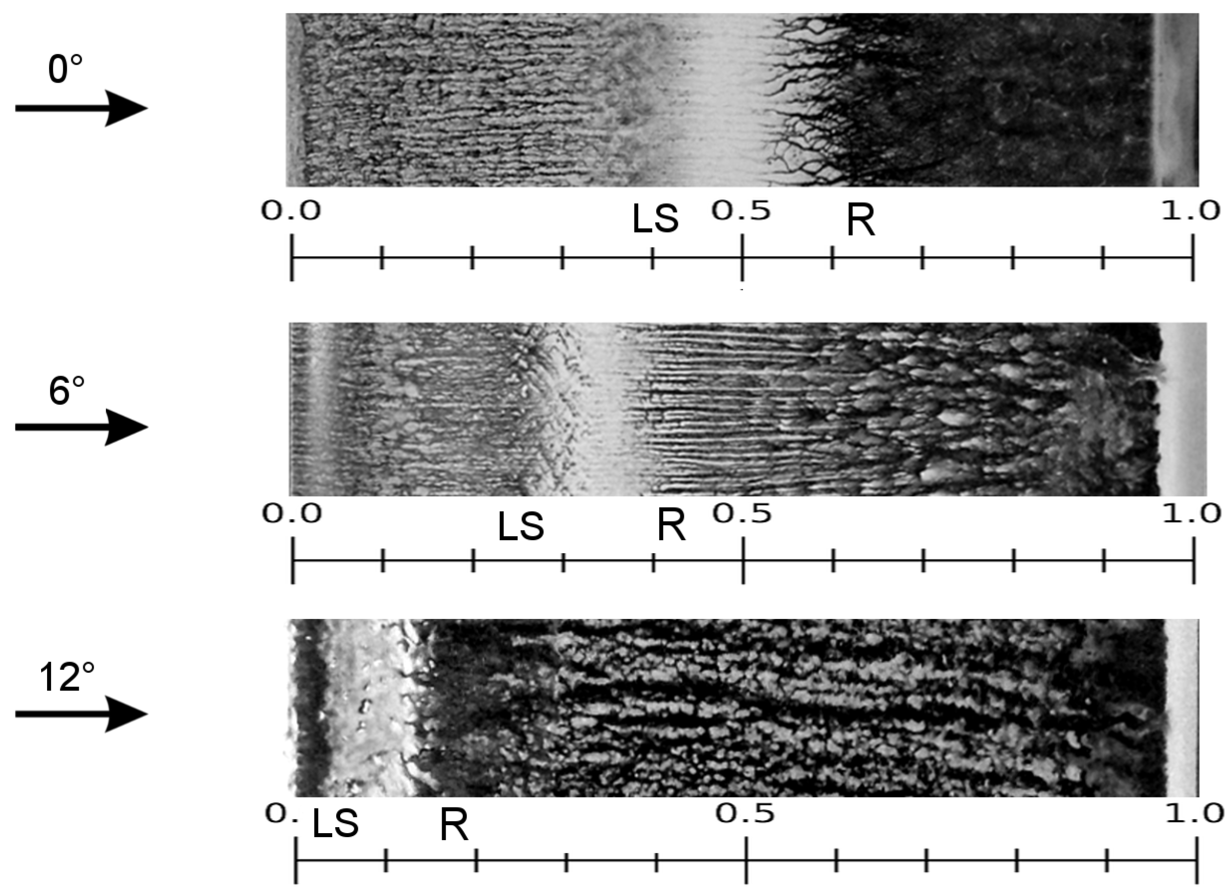
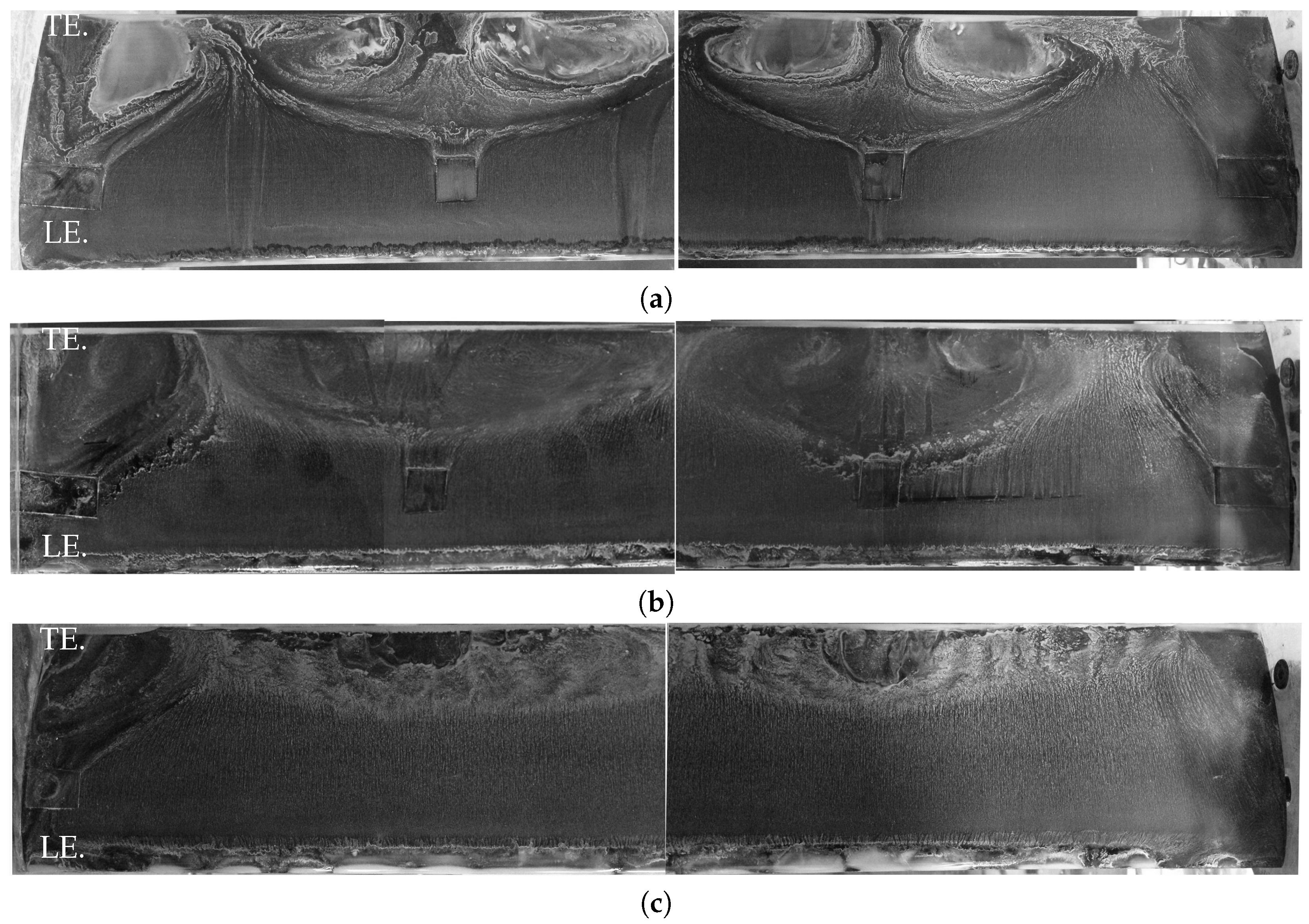
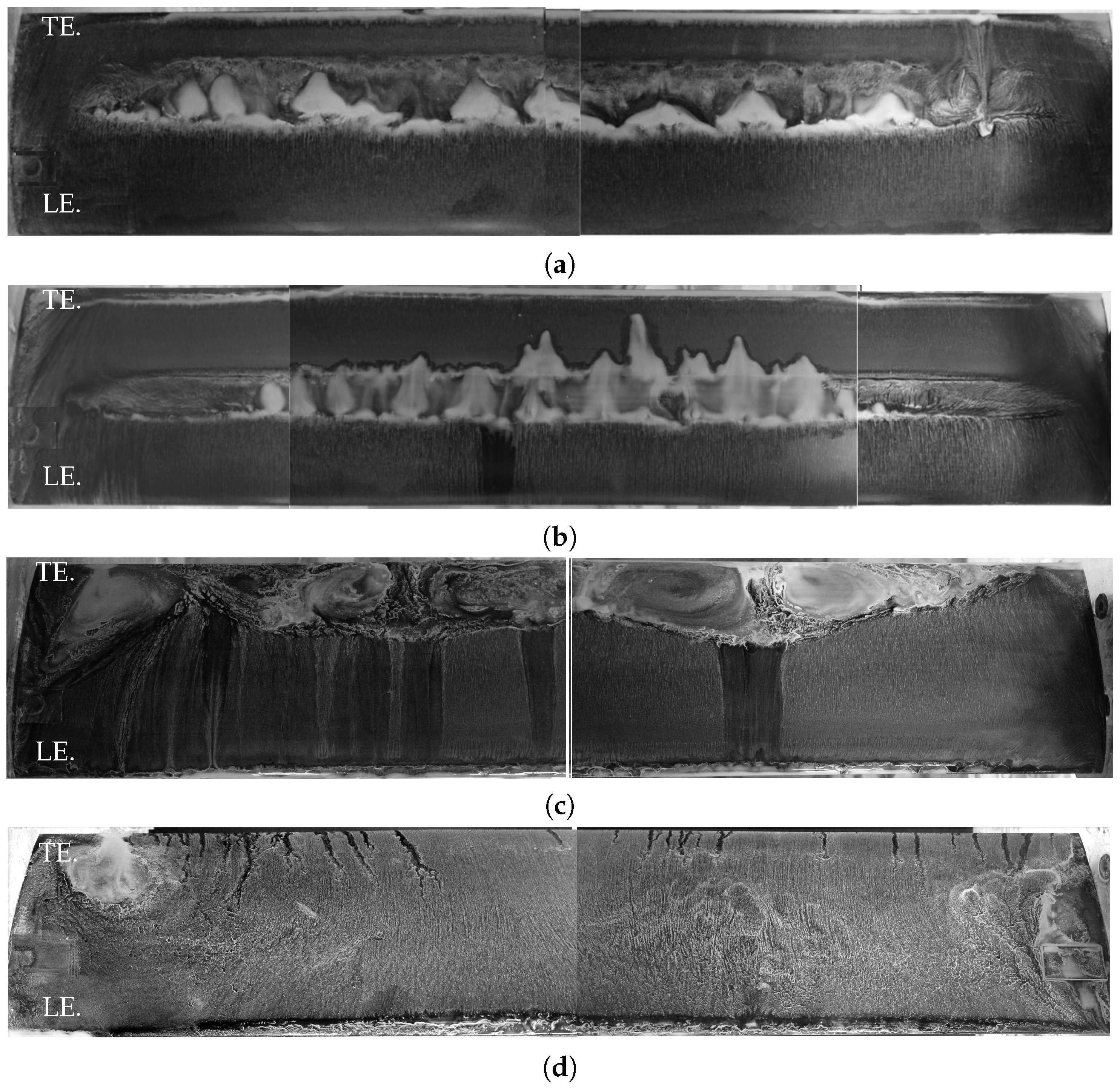
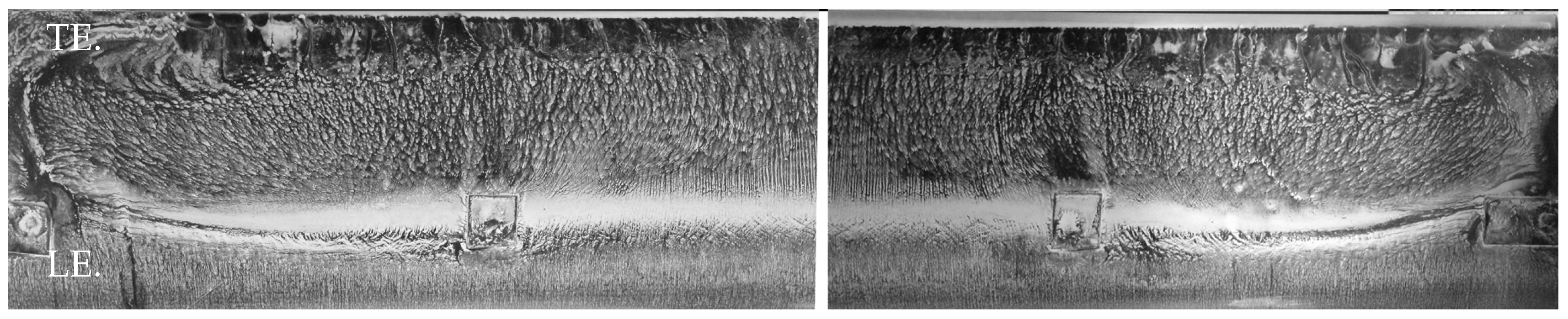
Surface Oil Flow Visualization

In connection with the above observations on the three-dimensionality of the flow, a surface oil flow visualization (SOFV) technique is used on the airfoil to study flow topology on the suction side of the airfoil. In order to prepare for the experiments, a visualization mixture with the components as presented in

Table 2. Components of the mixture used for surface oil flow visualization (SOFV) (per 100 g of the mixture).

Material	Composition	Amount
Titanium dioxide	TiO${}_2$	9 g
Talcum powder	Mg${}_3$Si${}_4$O${}_{10}$(OH)${}_2$	3 g
Kerosene	C${}_{12}$H${}_{26}$	40 g
Linseed oil *		16 g
Petroleum	C${}_{10}$H${}_{16}$	31 g
Oleic acid	C${}_{18}$H${}_{34}$O${}_2$	5 drops
Total		≈100 g

* No fixed formula exists for this. Linseed oil can polymerize into a solid form due to the distinctive reaction between one of its sub-components and oxygen in air. It is therefore used as a drying oil.

is sprayed on the airfoil surface.

Depending on the angle of attack and Reynolds number, the experimental time is adjusted for the mixture to dry out. The corresponding figures represent the oil traces at the end of each test. Subsequently, no time evolution of the flow is considered in this section. Figure 12 illustrates a visualization of stall cell formation performed in the present research with visible pairs of stall cells at Re = 160,000 near the stall angle of attack. This case has been chosen here for demonstration as it resulted in the clearest stall cell patterns. The flow passing from the leading edge (LE) towards the trailing edge (TE) undergoes a short separation and reattachment and later on separates due to geometrical constraints and strong pressure gradients. The shape and number of stall cells are governed by a combination of Reynolds number, the angle of attack and airfoil geometry (including aspect ratio).

As presented previously, strong low Reynolds number effects appear at Re = 40,000, particularly for angles of attack near stall. Figure 13 shows the evolution of the flow for increasing angles of attack ($\alpha =0^{\circ }$, $6^{\circ }$, ${12}^{\circ }$) at Re = 40,000. The presence of a laminar separation bubble (LSB) can be detected by an accumulation of white powder, which is observed for the three angles of attack. It is seen that the separation and reattachment locations (and hence, the LSB) move upstream towards the leading edge as the angle of attack increases. This is in agreement with the previous findings (e.g., Figure 5a).

Only portions of the span are presented in Figure 13, as the flow in most cases is two-dimensional at this Reynolds number; see Figure 14 for the case at $\alpha =6^{\circ }$. In this figure, the flow is directed from bottom to top, and the full span is represented by the junction of two pictures showing respectively the left and right parts of the span. Some wall effects in the form of corner vortices are observed; however, they do not impact the center of the test section where the pressure measurements were taken.

The 2D flow characteristics observed at Re = 40,000 for $\alpha =0^{\circ }$, $6^{\circ }$, ${12}^{\circ }$ and ${20}^{\circ }$ somewhat evolve at higher Reynolds numbers into large 3D structures. This is well visualized in Figure 15. Note that in order to have the possibility to separate the upper and lower surfaces of the airfoil, for accessing the pressure gauges, for example, the two surfaces were screwed together, leaving screw holes that can be treated as surface inhomogeneities or vortex generators, which can consequently initiate the formation of stall cells. In order to mitigate the effect of these disturbances, all measurements are performed by covering the screw holes in all experiments using plastic tape, which is a somewhat common practice. However, to minimize the effect of any disturbances, the airfoil surface holes have been made completely smooth by applying metal filler, and SOFV is performed for further investigation.

The Figure 15 also shows the flow visualizations at $\alpha ={12}^{\circ }$ for three cases to cross-compare the effects of both the Reynolds number and disturbances on the topology of the 3D structure: two cases with adhesive tape at Re = 160,000 and 100,000 and one case with filler at Re = 100,000. Compared to Figure 13, it can be seen that the location of the laminar separation and reattachment is now moved much further upstream towards the leading edge (indicated by the thick white lines at the leading edge). All cases develop distinct stall cells as well as the so called corner vortices near the wall. The figures also show that the tape pieces influence the shape of the stall cells; however, this is not the only reason for the generation of the stall cells (Figure 12 may be used to explain the physics further). Indeed, stall cells are observed even with the filler. They are present on a smaller portion of the chord, but their width is similar. As the tape pieces were influencing the flow, the following tests were performed with the tape filler.

Similar to Figure 13, the effect of the angle of attack is investigated in Figure 16 at a Reynolds number of Re = 200,000. As can be seen, both cases at $\alpha =0^{\circ }$ and $\alpha =6^{\circ }$ exhibit a laminar separation at about 50% and 40% of the chord, respectively, and a turbulent reattachment at about 80% and 60% of the chord. The laminar separation bubble becomes hence smaller and moves upstream as the angle of attack increases. However, no sign of stall cells is visible at such low angles of attack. At $\alpha ={12}^{\circ }$, two distinct pairs of vortices are visible in the middle of the airfoil span, and increasing the angle of attack to $\alpha ={20}^{\circ }$ results in the disappearance of the stall cell and the occurrence of leading edge separation.

Figure 17 illustrates the Reynolds number effects on the flow patterns on the airfoil by keeping the angle of attack constant at $\alpha ={12}^{\circ }$. As can be seen, no stall cells are created at Re = 40,000. At Re = 100,000 and 200,000; however, the patterns of stall cell are clear, and it can be seen that the strength of the stall cells increases and the vortex pairs near the trailing edge become more distinguishable as the Reynolds number increases. Another observation is that in Figure 16 and Figure 17, one can observe corner vortices whose magnitude increases with the angle of attack and Reynolds number.

4. Conclusions

Detailed experimental analysis of the NREL S826 airfoil at Reynolds numbers ranging from 40,000–200,000 was presented in this paper. In particular, surface pressure measurements were carried out for angles of attack of $0^{\circ }$, $6^{\circ }$, ${12}^{\circ }$ and ${20}^{\circ }$, respectively, and the flow patterns on the suction side of the airfoil were particularly studied to investigate the creation of separation bubbles, as well as the formation of the stall cells (mushroom structures) due to the 3D flow separation. The main findings of the current research are summarized below.

• The NREL S826 airfoil was experimentally investigated and detailed airfoil polars, pressure distribution, as well as surface flow visualizations were documented for future use as a reference.
• It was found that the separation point moves towards the leading edge when increasing the angle of attack and Reynolds number.
• Strong hysteresis effects were observed at Reynolds numbers lower than 100,000. The characteristics of the airfoil for higher Reynolds number flows are somewhat independent of the Reynolds number.
• No stall cells were found at Re = 40,000, but it was observed that increasing the Reynolds number may result in distinct vortex pairs, which are most visible around an angle of attack $\alpha ={12}^{\circ }$, close to the stall angle.
• Through upstroke and downstroke pitching of the airfoil, static stall hysteresis was found responsible for some of the complexities of the S826 airfoil at low Reynolds numbers, and a method for removing such effects based on inflow turbulence generation was tested successfully. It was found that the hysteresis strength has an inverse relation with the Reynolds number, and the effects diminish at Re = 100,000.
• The dependence of the flow patterns on the disturbances on the airfoil surface was investigated, and it was found that the presence of surface roughness results in more distinct vortex pairs on the suction side of the airfoil. However, disturbances themselves cannot promote the formation of stall cells.
• As mentioned in the Introduction, results presented in this article will be applicable to a wide range of low Reynolds number flows such as domestic and vertical axis wind turbines. Of particular interest is, nonetheless, the importance of 3D flow aerodynamics near the blade hub where the Reynolds numbers are smaller due to low speeds. The evolution of root vortices may be affected by the flow distribution and 3D effects stemming from the formation of stall cells. The interesting flow features in the root region, which consequently may affect the evolution of tip vortices, thereby influencing the wake behind turbines, have received little attention in the past, nor have they been addressed in the present article, but these flows will be studied in future research.

References

1. Bastankhah, M.; Porté-Agel, F. Wind tunnel study of the wind turbine interaction with a boundary-layer flow: Upwind region, turbine performance, and wake region. Phys. Fluids 2017, 29, 065105. [Google Scholar] [CrossRef]
2. Pierella, F.; Krogstad, P.Å.; Sætran, L. Blind Test 2 calculations for two in-line model wind turbines where the downstream turbine operates at various rotational speeds. Renew. Energy 2014, 70, 62–77. [Google Scholar] [CrossRef]
3. Bartl, J.; Sætran, L. Blind test comparison of the performance and wake flow between two in-line wind turbines exposed to different turbulent inflow conditions. Wind Energy Sci. 2017, 2, 55–76. [Google Scholar] [CrossRef] [Green Version]
4. Hu, H.; Yang, Z. An experimental study of the laminar flow separation on a low-Reynolds-number airfoil. J. Fluids Eng. 2008, 130, 051101. [Google Scholar] [CrossRef]
5. Choudhry, A.; Arjomandi, M.; Kelso, R. A study of long separation bubble on thick airfoils and its consequent effects. Int. J. Heat Fluid Flow 2015, 52, 84–96. [Google Scholar] [CrossRef]
6. Windte, J.; Scholz, U.; Radespiel, R. Validation of the RANS-simulation of laminar separation bubbles on airfoils. Aerosp. Sci. Technol. 2006, 10, 484–494. [Google Scholar] [CrossRef]
7. Selig, M. Low Reynolds number airfoil design lecture notes. In VKI Lecture Series; von Karman Institute for Fluid Dynamics: Sint-Genesius-Rode, Belgium, 2003; pp. 24–28. [Google Scholar]
8. Horton, H. Laminar Separation Bubbles in Two and Three Dimensional Incompressible Flow. Ph.D. Thesis, Queen Mary University of London, London, UK, 1968. [Google Scholar]
9. Sarlak, H. Large Eddy Simulation of an SD7003 Airfoil: Effects of Reynolds number and Subgrid-scale modeling. J. Phys. Conf. Ser. 2017, 854, 012040. [Google Scholar] [CrossRef] [Green Version]
10. Tani, I. Boundary-layer transition. Ann. Rev. Fluid Mech. 1969, 1, 169–196. [Google Scholar] [CrossRef]
11. Gaster, M. The Structure and Behaviour of Laminar Separation Bubbles; HM Stationery Office: Richmond, UK, 1969. [Google Scholar]
12. Winkelman, A.; Barlow, J. Flowfield model for a rectangular planform wing beyond stall. AIAA J. 1980, 18, 1006–1008. [Google Scholar] [CrossRef]
13. Rodríguez, D.; Theofilis, V. On the birth of stall cells on airfoils. Theor. Comput. Fluid Dyn. 2011, 25, 105–117. [Google Scholar] [CrossRef] [Green Version]
14. Manolesos, M.; Papadakis, G.; Voutsinas, S.G. Experimental and computational analysis of stall cells on rectangular wings. Wind Energy 2014, 17, 939–955. [Google Scholar] [CrossRef]
15. Manolesos, M.; Voutsinas, S.G. Geometrical characterization of stall cells on rectangular wings. Wind Energy 2014, 17, 1301–1314. [Google Scholar] [CrossRef]
16. Boiko, A.; Dovgal, A.; ZANIN, B.; Kozlov, V. Three-dimensional structure of separated flows on wings (review). Thermophys. Aeromech. 1996, 3, 1–13. [Google Scholar]
17. Yon, S.; Katz, J. Study of the unsteady flow features on a stalled wing. AIAA J. 1998, 36, 305–312. [Google Scholar] [CrossRef]
18. Broeren, A.P.; Bragg, M.B. Spanwise variation in the unsteady stalling flowfields of two-dimensional airfoil models. AIAA J. 2001, 39, 1641–1651. [Google Scholar] [CrossRef]
19. Ragni, D.; Ferreira, C. Effect of 3D stall-cells on the pressure distribution of a laminar NACA64-418 wing. Exp. Fluids 2016, 57, 127. [Google Scholar] [CrossRef]
20. Zarutskaya, T.; Arieli, R. On vortical flow structures at wing stall and beyond. In Proceedings of the 35th AIAA Fluid Dynamics Conference and Exhibit, Toronto, ON, Canada, 6–9 June 2005; pp. 1–10. [Google Scholar]
21. Shur, M.; Spalart, P.R.; Squires, K.D.; Strelets, M.; Travin, A. Three dimensionality in Reynolds-averaged Navier–Stokes solutions around two-dimensional geometries. AIAA J. 2005, 43, 1230–1242. [Google Scholar] [CrossRef]
22. Manni, L.; Nishino, T.; Delafin, P.L. Numerical study of airfoil stall cells using a very wide computational domain. Comput. Fluids 2016, 140, 260–269. [Google Scholar] [CrossRef]
23. Sarlak, H.; Nishino, T.; Sørensen, J.N.; Simos, T.; Tsitouras, C. URANS simulations of separated flow with stall cells over an NREL S826 airfoil. AIP Conf. Proc. 2016, 1738, 030039. [Google Scholar] [CrossRef] [Green Version]
24. Sarlak, H.; Meneveau, C.; Sørense, J. Role of subgrid-scale modelling in large eddy simulation of wind turbine wake interactions. Renewable Energy 2015, 77, 386–399. [Google Scholar] [CrossRef]
25. Frère, A.; Hillewaert, K.; Sarlak, H.; Mikkelsen, R.; Chatelain, P. Cross-validation of numerical and experimental studies of transitional airfoil performance. In Proceedings of the 33rd Wind Energy Symposium, Kissimmee, FL, USA, 5–9 Janurary 2015; American Institute of Aeronautics & Astronautics: Reston, VA, USA, 2015. [Google Scholar]
26. Sagmo, K.; Bartl, J.; Sætran, L. Numerical simulations of the NREL S826 airfoil. J. Phys. Conf. Ser. 2016, 753, 082036. [Google Scholar] [CrossRef]
27. Sarlak, H. Large Eddy Simulation of Turbulent Flows in Wind Energy. Ph.D. Thesis, Technical University of Denmark, Lyngby, Denmark, 2014. [Google Scholar]
28. Sarlak, H.; Mikkelsen, R.; Sarmast, S.; Sørensen, J. Aerodynamic behaviour of NREL S826 at Re = 100,000. J. Phys. Conf. Ser. 2014, 524, 012027. [Google Scholar] [CrossRef]
29. Ross, I.; Altman, A. Wind tunnel blockage corrections: Review and application to Savonius vertical-axis wind turbines. J. Wind Eng. Ind. Aerodyn. 2011, 99, 523–538. [Google Scholar] [CrossRef]
30. Barlow, J.; Rae, W.; Pope, A. Low-Speed Wind Tunnel Testing; Wiley: New York, NY, USA, 1999. [Google Scholar]
31. Sumer, B.M. Hydrodynamics Around Cylindrical Strucures; World Scientific: Singapore, 2006; Volume 26. [Google Scholar]
32. Mittal, S.; Saxena, P. Prediction of hysteresis associated with static stall of an airfoil. AIAA J. 2000, 38, 933–935. [Google Scholar] [CrossRef]
Figure 1. A sketch of the wind tunnel facility at the Technical University of Denmark. (a) Wind tunnel and data processing systems; (b) test section.
Energies 11 01418 g001
Figure 2. The S826 airfoil model and the pressure tap locations. The points shown by the dashed line are not instrumented, and the pressure data are interpolated for these locations based on the neighboring pressure tap values.
Energies 11 01418 g002
Figure 3. Measured lift (left) and drag (right) coefficients for the S826 airfoil at various Reynolds numbers. Lift values are obtained using a force gauge and drag is obtained by integrating the velocity deficit at the wake rake location. Curves of the same color and angle of attack indicate upstroke and downstroke pitching. A discrepancy between the same lines, therefore, indicates static stal hysteresis at the specific angle.
Energies 11 01418 g003
Figure 4. Comparison of the measured lift and drag distributions with and without wind tunnel correction. Circles show the uncorrected measured data, and stars show the corrected measurement.
Energies 11 01418 g004
Figure 5. Pressure distribution on the suction side of the S826 airfoil at Reynolds numbers Re = 40,000, 100,000, 150,000 and 200,000. The standard deviation is plotted using error bars. (a) Re = 40,000; (b) Re = 100,000; (c) Re = 150,000; (d) Re = 200,000.
Energies 11 01418 g005
Figure 6. Uncertainty (standard deviation) of surface pressure measurements over the entire range of angles of attack at Reynolds numbers Re = 40,000, 100,000, 150,000 and 200,000. (a) Re = 40,000; (b) Re = 100,000; (c) Re = 150,000; (d) Re = 200,000.
Energies 11 01418 g006
Figure 7. The effects of wires of various thickness in generating downstream turbulence in the wind tunnel. (a) Wire setup used.; (b) turbulence intensities alongside the tunnel (C: chord, LE and TE: leading and trailing edges) with wires in place.
Energies 11 01418 g007
Figure 8. Instantaneous and time averaged wake velocities showing the effects from added turbulence. The Reynolds number is 40,000, and the legend indicates which free stream turbulence cases are being run.
Energies 11 01418 g008
Figure 9. Effect of added turbulence in lift coefficients at (a) Re = 40,000 and (b) Re = 100,000, respectively. Each marker color shows a full circle of measurements at a Reynolds number, while the hollow and filled circles of the same color represent the upstroke and downstroke pitching, respectively.
Energies 11 01418 g009
Figure 10. Effect of added turbulence in pressure distribution at (a) Re = 40,000 and (b) Re = 100,000. For clarity, the downstroke pitching is not shown. The three points shown by upward-pointing double arrows on the horizontal axes of pressure distribution subfigures are found by interpolating/extrapolating the neighboring points, as it was not possible to make measurements at those points due to machining and size limitations.
Energies 11 01418 g010
Figure 11. Investigation of 3D flow effects: comparison of lift coefficients using pressure integration ( C l p ) and force gauge ( C l g ) at Reynolds numbers 40,000 and 200,000. (a) Re = 40,000; (b) Re = 200,000.
Energies 11 01418 g011
Figure 12. Visualization of stall cells formed over the S826 airfoil at Re = 160,000 and α = 12 .
Energies 11 01418 g012
Figure 13. visualization of the Laminar Separation (LS) and Reattachment (R) positions for different angles of attack ( α = 0 , 6 and 12 ). Top view on a mid-span section of the suction side for Re = 40,000.
Energies 11 01418 g013
Figure 14. Flow visualization on the suction side at Re = 40,000 and α = 6 . Flow going from bottom to top. Two pictures (left and right) are combined to form a visualization along the full span.
Energies 11 01418 g014
Figure 15. The effect of disturbances on the stall cell patterns at α = 12 . Flow is passing from bottom (LE) to top (TE). (a) Re = 160,000 and α = 12 : screw holes covered by tape; (b) Re = 100,000 and α = 12 : screw holes covered by tape; (c) Re = 100,000 and α = 12 : screw holes covered by filler.
Energies 11 01418 g015
Figure 16. Effect of increasing the angle of attack on stall cell flow patterns for Re = 200,000. Flow is directed from bottom (LE) to top (TE). (a) Re = 200,000 and α = 0 ; (b) Re = 00,000 and α = 6 ; (c) Re = 200,000 and α = 12 ; (d) Re = 200,000 and α = 20 .
Energies 11 01418 g016
Figure 17. Effect of increasing the Reynolds number near stall ( α = 12 ) on stall cell patterns. Flow is directed from bottom (LE) to top (TE). (a) Re = 40,000; (b) Re = 100,000; (c) Re = 200,000.
Energies 11 01418 g017