Time-Domain Voltage Sag State Estimation Based on the Unscented Kalman Filter for Power Systems with Nonlinear Components


1
División de Estudios de Posgrado, Facultad de Ingeniería Eléctrica, Universidad Michoacana de San Nicolás de Hidalgo, Av. Francisco J. Múgica S/N, Morelia, Michoacán 58030, Mexico
2
Institute for Energy and Environment, Department of Electronic and Electrical Engineering, University of Strathclyde, 204 George Street, Glasgow G1 1RX, UK
*
Author to whom correspondence should be addressed.
Energies 2018, 11(6), 1411; https://doi.org/10.3390/en11061411
Submission received: 1 May 2018
/
Revised: 17 May 2018
/
Accepted: 23 May 2018
/
Published: 1 June 2018
(This article belongs to the Special Issue Power Quality in Microgrids Based on Distributed Generators)
Abstract
:This paper proposes a time-domain methodology based on the unscented Kalman filter to estimate voltage sags and their characteristics, such as magnitude and duration in power systems represented by nonlinear models. Partial and noisy measurements from the electrical network with nonlinear loads, used as data, are assumed. The characteristics of voltage sags can be calculated in a discrete form with the unscented Kalman filter to estimate all the busbar voltages; being possible to determine the rms voltage magnitude and the voltage sag starting and ending time, respectively. Voltage sag state estimation results can be used to obtain the power quality indices for monitored and unmonitored busbars in the power grid and to design adequate mitigating techniques. The proposed methodology is successfully validated against the results obtained with the time-domain system simulation for the power system with nonlinear components, being the normalized root mean square error less than 3%.
1. Introduction
Power quality (PQ) is an important operation issue in any power system. Utilities must comply with strict standards, relating primarily harmonics, transients and voltage sags [1,2,3,4]. PQ depends on the power supply, the transmission and distribution systems and the electrical load condition. Voltage sags are among the adverse PQ effects; they can cause malfunction of electronic loads, and can reset voltage-sensitive loads [5,6]. The voltage sags characteristics in magnitude and duration are necessary to determine their effect in the grid and its loads. They constitute the majority of PQ problems, representing about 60% of them [7,8]. Among the problems that the nonlinear electrical components introduce to the power grid is the increase of harmonic distortion, which is an important effect to mitigate. Voltage sags have increased due to the use of nonlinear varying loads such as power electronic devices, smelters, arc furnaces and electric welders, the starting of large electrical loads, switching transients, connection of transformers and transmission lines, network faults, lightning strikes, network switching operations, among others [9].
The Kalman filter (KF) and the least squares methods have been used to estimate the voltage fluctuations in linear power systems [10,11,12,13]. PQ state estimation based on the KF uses a linear model, partial and noisy measurements from the system. In [14] the number of sags is estimated using a limited number of monitored busbars, recording the number of voltage sags during a determined period.
This research work proposes as an innovation, an alternative methodology based on the unscented Kalman filter (UKF) to perform the voltage sags state estimation (VSSE) in nonlinear load power networks; this method can also be applied to nonlinear micro grids. The VSSE determines the magnitude, duration and beginning-ending time of sags, with an observable system condition for the busbars voltages using the available measurements.
The KF has been applied to estimate harmonics and voltage transients in a signal [15], KF gain can be modified during the state estimation to reduce the estimation error [16], both references assess linear cases; [17] has proposed the UKF to detect sags in a voltage waveform. In this work, the UKF is extended to the nonlinear case to solve the time-domain VSSE, to estimate voltage sags in all busbars of a power system including nonlinear components. The UKF makes use of a power grid nonlinear model and noisy measurements from the same electrical network to estimate all the busbar voltages.
The extended Kalman filter (EKF) can be also applied to solve the nonlinear state estimation. The UKF error is slightly smaller when compared to the EKF error. This state estimation error increases in the filters when sudden variations are present, both being of about the same accuracy. The EKF can lead to divergence more easily than UKF, which shows good numerical stability properties.
The state estimation receives measurements from the power network, through a wide area measurement system (WAMS) and estimates the state vector, using algorithms such as the UKF. Practical implementation of the time-domain state estimation can be achieved with measuring instruments and data acquisition cards, capable of recording the voltage and current waveforms synchronously during several cycles, e.g., using the global positioning system (GPS) to time stamp the measurements [18,19,20,21]. The use of adequate communication channels like especially dedicated optical fibre links, allows to the measurements be sent to the control centre with high data updating rate, where they are received and numerically processed using computational systems with sufficient memory and adequate capability [9].
Due to economic reasons measurement technology for VSSE is currently limited, making the system underdetermined. The VSSE presents different problems from those of the traditional power system state estimation, where redundancy of measurements is possible [22].
The VSSE has been assessed in the frequency domain [14,23]. In this work, the UKF is proposed as an alternative method to obtain the time-domain VSSE. This approach makes possible the use of nonlinear models to represent more accurately the power system components and to obtain the results with a low state estimation error. The state estimation obtains the global or total system state that can be used to take corrective actions to mitigate the adverse effects of voltage sags, such as the network configuration change or control of flexible alternating current transmission system (FACTS) devices, e.g., the static synchronous compensator (STATCOM).
The time-domain UKF state estimation methodology can be used not only to estimate voltage sags but also to estimate over voltages, over currents or electromagnetic transients. The main objective of this work is to apply the UKF to obtain the VSSE, by addressing the dynamics of the nonlinear electrical networks and by estimating and delimiting the voltage sags in the time-domain. The case studies address short circuit faults and transient load conditions. The results are validated against the actual time-domain response of the power grid.
2. Dynamic State Estimation
The network model can be a set of first order differential equations to describe the dynamic state performance. The dynamic estimation data are the grid model with its inputs and a measurement set of selected outputs from the system during a determined number of cycles to define the measurement equation.
The KF dynamically follows the variations in the states, i.e., currents and voltages, detecting changes in the voltage waveform within less than half of a cycle and it is a good tool for instantaneous tracking and detection of voltage sags [24,25].
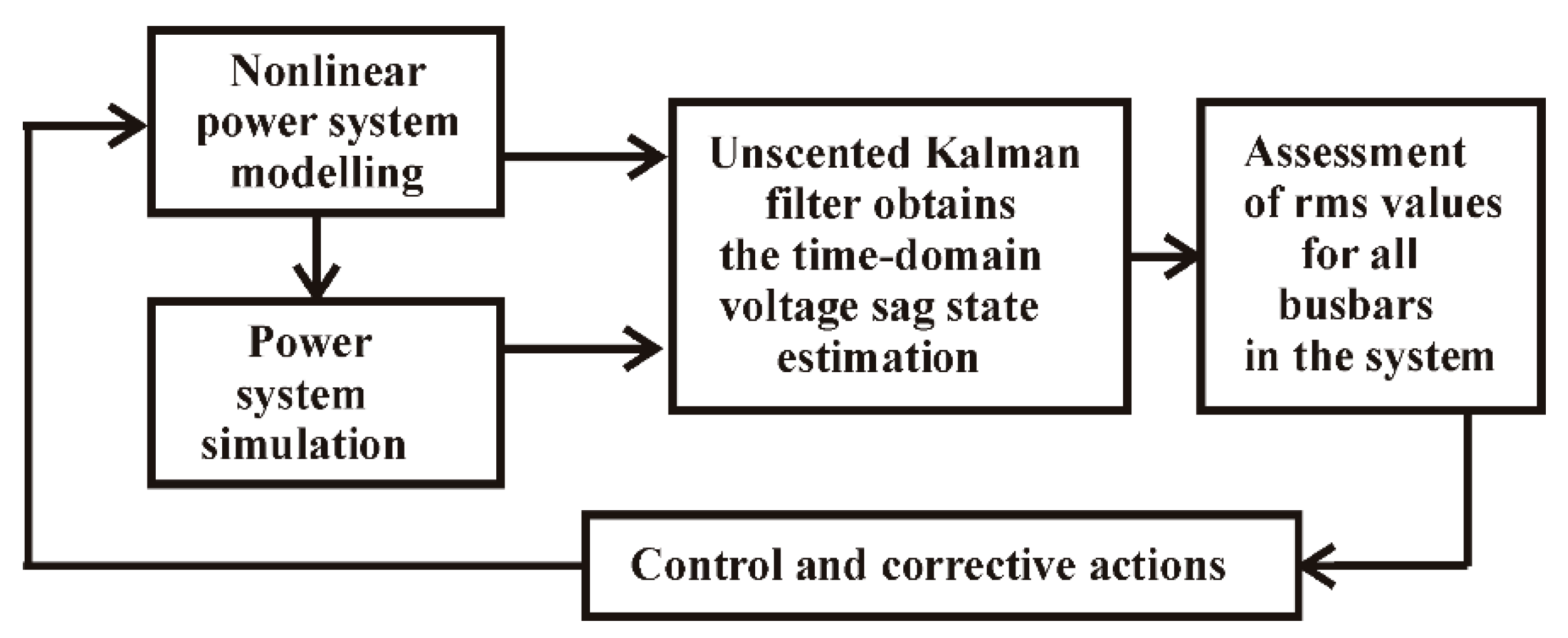
The KF solves the dynamic estimation, due to its recursive process [26,27]; being applied in linear cases. The UKF solves the dynamic estimation in nonlinear cases. In this work, the UKF estimates the nonlinear power system state under transient conditions, e.g., voltage sags [28]. Figure 1 describes the proposed VSSE methodology. The main steps are the nonlinear power system modelling and simulation, then UKF is applied to obtain the time-domain VSSE, and lastly the assessment of rms busbar voltages.
The UKF applies a deterministic sampling technique; i.e., the unscented transform (UT), which takes a set of sigma points near of their mean value. These points are propagated through the nonlinear model by evaluating the estimated mean and covariance [25]. The mean and covariance are encoded in the set of sigma points; these points are treated as elements of a discrete probability distribution, which has mean and covariance equal to those originally given. The distribution is propagated by applying the non-linear function to each point. The mean and the covariance of the transformed points represent the transformed estimate.
The main advantage of the UKF is the derivative free nonlinear state estimation, thus avoiding analytical or numerical derivatives [29,30]. The UT avoids the need of linearization using the Jacobian matrix as in the EKF, and it can be applied to any function, independently if it is differentiable or not. The UKF includes a Cholesky decomposition with an inverse matrix to evaluate the sigma points at each time step.
Inaccuracies of the model and its parameters can be taken into account with a statistical term w, called noise process. It accounts for the existence of phenomena such as the thermal noise of the electrical elements and the ambiguity in the accuracy of the parameters. Metering devices have errors and noise; they are represented by a statistical term v. In most cases, w and v have a Gaussian distribution. UKF is able to operate with partial, noisy, and inaccurate measurements [31,32].
3. Unscented Kalman Filter Methodology
The UT is based on the mean and covariance propagation by a nonlinear transform. The system and measurement nonlinear models can be represented as:
where is the state vector, u the known input vector of variable order, y the variable order output vector, f a nonlinear state function and h is a nonlinear output function, with n states and m measurements.
UKF uses a deterministic approach for mean and covariance calculation; 2n + 1 sigma points are defined by using a square root decomposition of prior covariance. Sigma points propagation through the model (1) obtains the weighted mean and covariance. Wi represents the scalar weights, defined as:
where λ and γ are scaling parameters, α and κ determine the spread of sigma points; β is associated with the distribution of x. If Gaussian β = 2 is optimal, α = 10−3 and κ = 0 are normal values [30].
UT takes the sigma points with their mean and covariance values, and transform them by applying the nonlinear function f, and then the mean and covariance can be calculated for the transformed points. A weight Wi is assigned to each point.
UKF defines the n-state discrete-time nonlinear system from (1) and (2) as:
Process noise w and measurement noise v are assumed stationary, zero-averaged and uncorrelated, and are the covariance matrices for noises w and v, respectively.
UKF applies the following steps:
(a) Initialization, k = 0.
E is the expected value, P is the error covariance matrix, + indicates update estimate or a posteriori estimate and − project estimate or a priori estimate. Subscripts k and k − 1 denote time instants tk = k∆t and tk−1 = (k − 1)∆t, respectively, ∆t is the time step.
(b) Sigma points assessment in matrix form by columns:
(c) Update time step k from k − 1.
matrix represents the sigma points; matrix represents the updated sigma points and the updated output vector with sigma points.
(d) Evaluate the error covariance matrices as:
(e) UKF algorithm evaluates the filter gain Kk and updates the estimated state and the error covariance matrix.
The steps (b)–(d), Equations (14)–(22), define the prediction stage, and the last step (e), Equations (23)–(25), defines the update stage, as in the KF algorithm [33,34]. The main objective of this work is to use the UKF formulation to estimate the busbar voltage waveforms, mainly at unmonitored busbars in the presence of voltage sags generated by faults and load transients.
Waveforms can be contaminated with noise, and the assumption of constant values for Q and R is valid when the noise characteristics are constant, like its standard deviation and variance. If the noise is varying, Q and R should be computed at each time step and an adaptive KF is a requirement [16]. UKF algorithm tracks the time-varying model and noise through the on-line calculation of Q and R. In this work, Q and R matrices are assumed constant, in order to mainly analyse the UKF application to time-domain VSSE.
UKF identifies the interval where the sags are present, as well as their magnitude, with an acceptable precision. By increasing the number of cycles, the UKF can identify the voltage characteristics during fault transient periods.
The number of points per cycle is of important concern to evaluate the time-domain state estimation with periodic signals. This number defines the sampling rate for the monitored signals. The sampled waveform is a sequence of values taken at defined time intervals and represents the measured variable. Interpolation can be used to adjust the number of points per cycle, linearly or nonlinearly [35]. In addition, the interpolation should be used carefully with discrete signals to satisfy the sampling theorem. The sampling rate defines the speed at which the input channels are sampled; this rate is defined in samples per cycle. To detect transients, high sampling rates compared with the fundamental frequency may be necessary [36].
Rms Value of Discrete Waveforms and Normalized Root Mean Square Error
The rms voltage magnitude can be determined by processing the discrete values for the voltage waveform according to the used data window size and the sampling frequency. The rms voltage magnitude Vrms for a discrete voltage signal can be calculated as:
where Vj is the sample voltage j and N is the number of samples per cycle taken in the sampling window; i is the sampled cycle. This expression can be applied to discrete voltage and current waveforms [22].
Normalized root mean square error (NRMSE) is used to validate the UKF-VSSE methodology; this error evaluates the state estimation residual between actually observed values and the estimated values; lower residual indicates less state estimation error. NRMSE is defined as:
is the estimated vector, y is the real or actually observed vector and np the number of elements of these vectors.
4. Case Studies
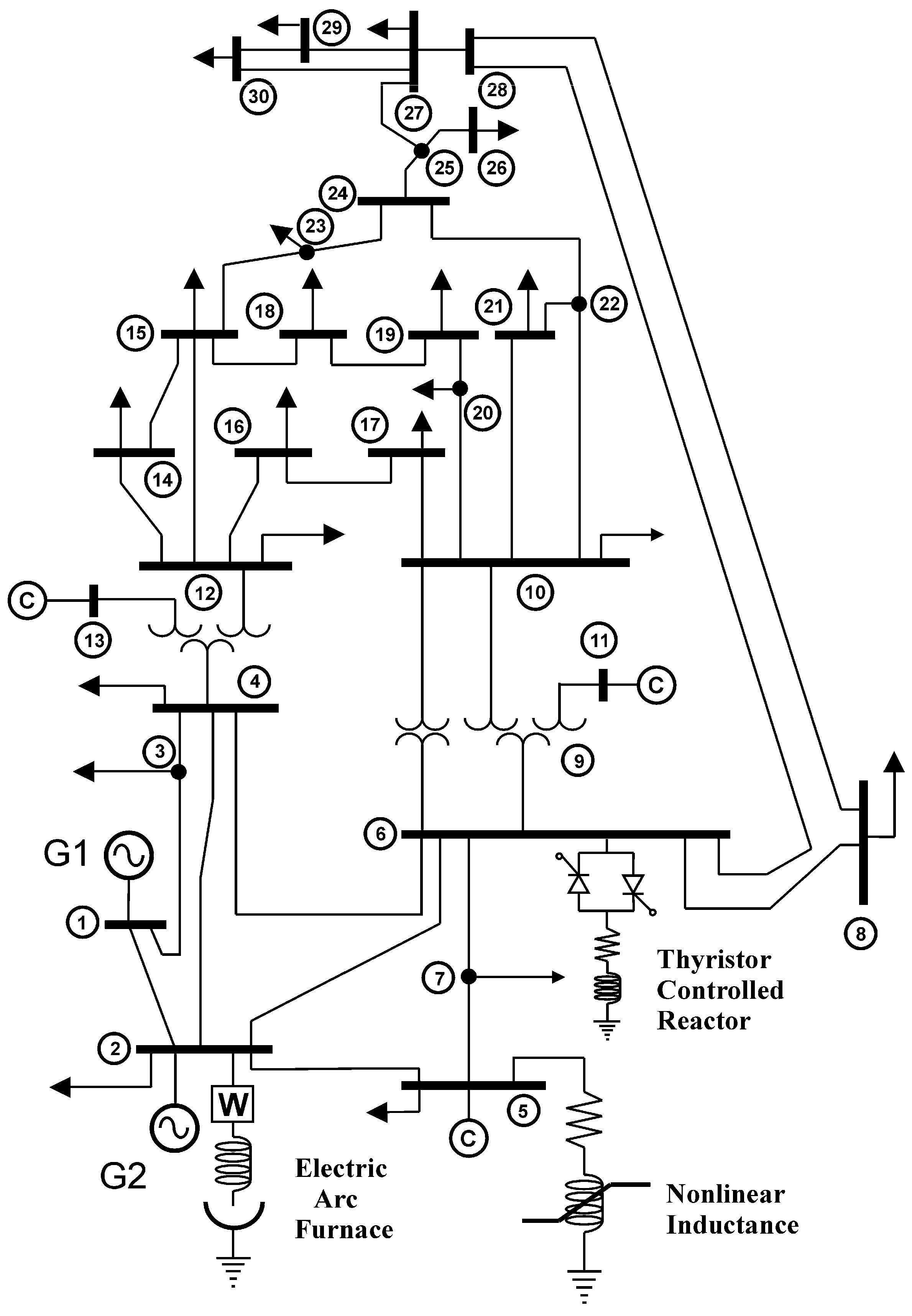
Figure 2 shows the modified IEEE 30-bus test system used in the case studies described next, assuming a three-phase base power of 100 MVA and a phase-to-phase base voltage of 230 kV. Lines 1–2, 1–4, 2–4, 2–5, 2–6, 4–6 and 5–6 are represented by an equivalent pi model and by series impedance the rest of lines; transformers 6–10, 4–12–13, 6–10–11, are represented by an inductive reactance, according to the IEEE 30-bus test power system [37].
The system is modified adding three nonlinear electrical loads, i.e., an electric arc furnace (EAF) to busbar 2, a nonlinear inductance to busbar 5 and a thyristor-controlled reactor (TCR) to busbar 6. The addition of these nonlinear elements gives the nonlinearity of (1) and (2). Appendix A gives additional parameters of nonlinear loads. Appendix B presents the nonlinear load models and their differential equations.
Generators are modelled as voltage sources connected to busbars through a series inductance. Linear electric loads are represented as constant impedances. Busbar voltages, line and load currents are defined as state variables to obtain the state space model for the power network; the measurements are function of these state variables.
The measurement locations are selected so that the busbar voltages are observable. Table 1 and Table 2 show x and z vectors, respectively, to form the measurement equation by obtaining 103 measurements to estimate 110 state variables (n = 110, m = 103). The observation equation with this set of measurements has an underdetermined condition, but all the busbar voltages are observable to estimate the voltage sags. When busbar voltages are assessed and estimated other variables can be calculated, i.e., line currents or the TCR current.
The EAF real power and the nonlinear inductance current are included as nonlinear functions in the measurement equation (z = Hx) represented in the formulation by (2).
In the measurement matrix , each measurement is associated with its corresponding state variable (Table 2). The sampling frequency is at least 30.72 kHz, to obtain 512 samples per cycle, for a fundamental frequency of 60 Hz [24].
The conventional trapezoidal rule is used to solve the 110 first order ordinary differential equations set. To represent the power system, busbar voltages, line and load currents are defined as state variables; a step size of 512 points per period is used, i.e., 32.5 microseconds. The simulation time is set to 0.4 s or 24 cycles. The measurements are taken from this simulation and then are contaminated using randomly generated noise.
4.1. Case Study: UKF VSSE Short-Circuit Fault at Busbar 4
A transient condition is simulated by applying a single-phase to ground fault at busbar 4. The fault impedance is of 0.1 pu, to simulate a short-circuit fault, starting in cycle 13 (0.216 s) and ending in cycle 17 (0.283 s). This fault generates busbar voltage sags and swells, which can be estimated with the power network model, partial and noisy measurements from the system, and the UKF algorithm. The criterion to select this case study is to represent a transient fault in the transmission system and verify the proposed VSSE method.
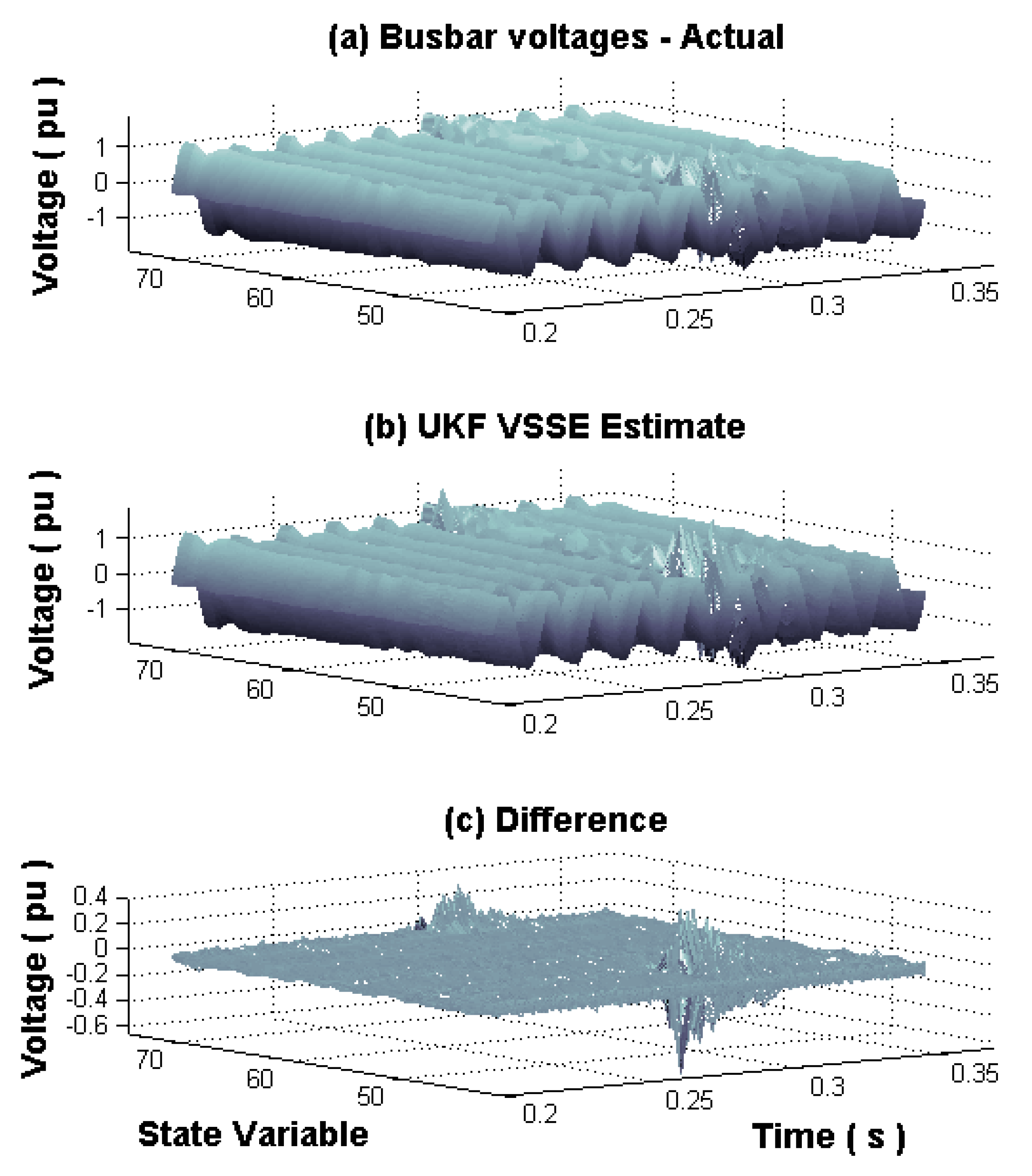
Measurement noise is assumed with a signal to noise ratio (SNR) of 0.025 pu or 2.5%; while a SNR of 0.001 pu or 0.1% is assumed for the noise process. Figure 3 shows the busbar voltages 1–30, where the actual, the proposed UKF estimate and the difference between instantaneous values during the fault at busbar 4 are shown, corresponding to state variables 42–71.
The largest estimation error is present when the fault condition is removed at 0.283 s; this error is due to sudden changes in the busbar voltages. It is approximately 7%, but quickly decreases in the next three cycles to 1%. These voltage fluctuations are due to the short-circuit transient condition at busbar 4.
Voltage waveforms for the faulted busbar 4 and for busbar 6, near to fault, are shown in Figure 4. Actual, UKF estimation and residual waveforms are illustrated. The presence of a voltage sag/swell condition at these busbars can be observed. Voltage sag lasts 4 cycles, while the fault condition is present, originating a reduction in the voltage magnitude of 12% for busbar 4 and 8% for busbar 6. Post-fault period begins at cycle 18, when the short circuit fault is removed. A voltage swell condition is present with a duration of two cycles and then the voltage eventually reaches the steady state. Residuals take considerable values during the voltage swell condition, the first two cycles of the post-fault period, and are due to the fast fluctuations of the state variables.
In Figure 4, NRMSE has been calculated using (27) to evaluate the state estimation error between actual and UKF estimated waveforms for the voltage busbars 4, and 6, during the 24 cycles under analysis, resulting on 2.5% and 1.2%, respectively.
Busbars 3–30 show a similar behavior as for busbars 4 and 6 during and after the short-circuit fault. The busbar voltage magnitude reduction mainly depends on the network topology, the load condition and the line impedance between the busbars. Fluctuations in the voltage waveforms at busbars are due to noisy measurements, network modelling, and the short-circuit fault used for the voltage sag/swell transient state estimation.
Line currents are shown in Figure 5 for the actual, UKF estimate and difference, respectively; with the fault condition at busbar 4 from 0.216 to 0.283 s.
The distribution of line currents in the power system is shown for the interval of study. This distribution represents the fault currents from generators to the faulted busbar 4, which can be observed in Figure 5 by the current fluctuations in the first state variables during and after the fault period. During the first cycle after fault clearance, the error increases to 12%, but once, this cycle ends the error decreases to around 1% in the post-fault period. The difference graph (c) presents this error at 0.283 s for the state variables representing the currents from generators to the faulted busbar 4.
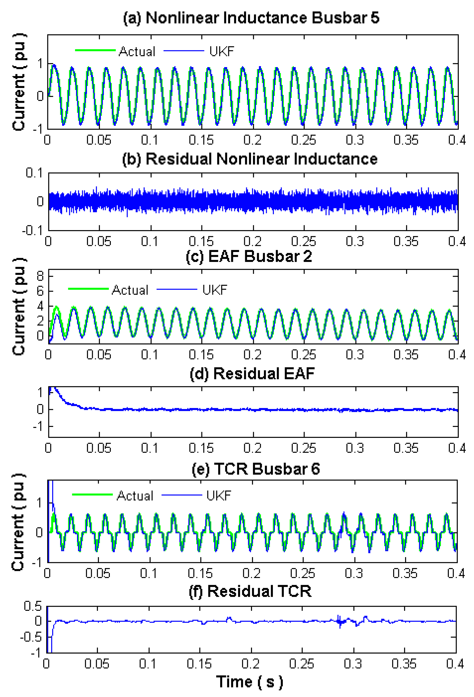
Actual, UKF estimated currents and residuals of nonlinear components are illustrated in Figure 6, for the nonlinear inductance (a,b), the EAF (c,d) and the TCR (e,f).
These state variables show small variations for the considered fault condition. Only in the post-fault period, TCR current differs by approximately 2.5%, but this difference decreases quickly after one cycle to negligible proportions, i.e., approximately to 1%. This error is due to the fast changes in the state variables which make the numerical process of state estimation difficult. The NRMSE between actual and UKF estimated waveforms for nonlinear load currents in Figure 6 gives 0.8% for the nonlinear inductance, 1.35% for the EAF, and 2.16% for the TCR.
4.2. RMS Busbar Voltages under the Short-Circuit Fault at Busbar 4
The voltage sags can be detected directly from the instantaneous or rms values of the nodal voltage waveforms, which are defined as state variables, by comparing the voltage values in the time interval under analysis. If these values vary, a voltage fluctuation (sag or swell) occurs.
Figure 7 shows the rms voltage magnitude for the faulted busbar 4 and for busbars 3, 6, 9, 12 and 14; these busbars are near to busbar 4 and present the largest voltage sags.
The rms magnitude of these voltages is computed using (26), the initial step when the voltage sag begins is due to the short-circuit fault; this time is at cycle 13 or 0.216 s. During the first cycle of post-fault period (cycle 18 or 0.283 s), a noticeable difference is present in the rms voltage of the nearby busbars. The largest difference is 20% for busbar 6, but this error is reduced drastically in the next cycle to 4.5%, being of negligible proportions during the following cycles (approximately 1%). This effect is due to sudden variations in the state variables during and after the fault is removed, which are difficult to follow exactly with the UKF algorithm.
Table 3 shows the actual and estimated voltage sags at the network busbars, referred to the pre-fault magnitudes, due to the single-phase to ground fault at busbar 4. These values are computed again using (26); not listed busbars have a voltage variation of less than 0.01 pu during the fault. The magnitude of the estimated voltage sags closely matches the actual values, thus validating the proposed UKF VSSE methodology.
4.3. Case Study: UKF VSSE Single-Phase to Ground Fault at Busbar 15
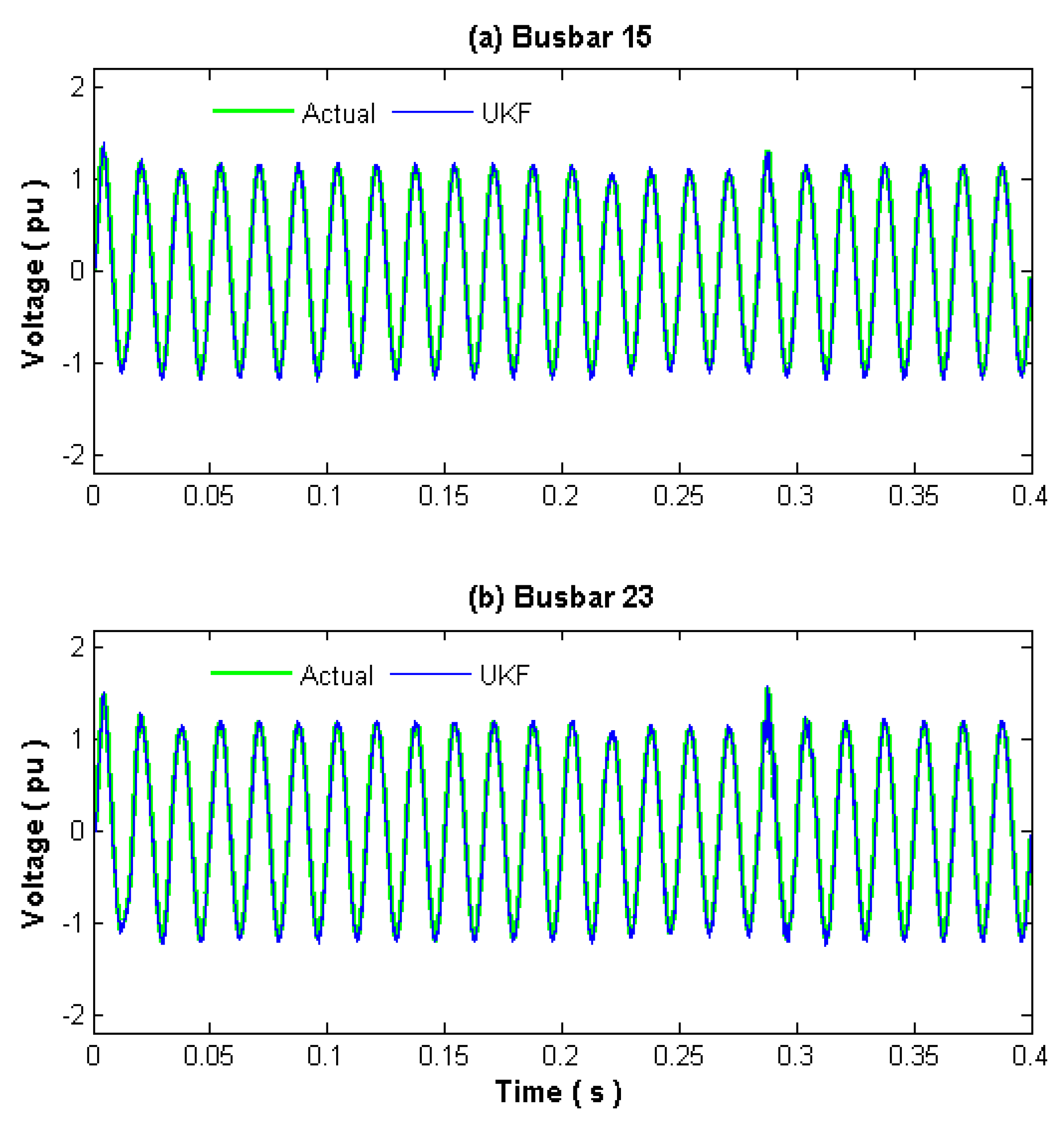
This case study reviews the UKF VSSE when a single-phase to ground fault is applied at busbar 15; the fault impedance is 0.35 pu. This impedance is used to decrease the fault effect in the transient system condition. Busbar 15 has no voltage measurement, however, the state estimation is able to assess its voltage and the voltage of the nearby busbars with the same measurement points of the previous case. Measurements are contaminated with a 2.5% SNR noise. This case study is addressed to represent a short-circuit in the distribution network to assess the VSSE. The state estimation assessment of high power load switching can be also addressed. Figure 8 shows results under the short-circuit fault condition for busbar voltages 15 and 23; these are the busbars that present the largest voltage sag during the examined transient condition.
A close agreement between the actual and UKF estimated signals including the post-fault period is achieved. Note the swell condition after the fault period. The UKF NRMSE for voltage at busbars 15 and 23 are 1.5%, and 0.65%, respectively.
Figure 9 shows the rms busbar voltages near of the busbar 15. The proposed UKF algorithm gives acceptable estimates for the voltage sag magnitude and duration, mainly for the transient starting and ending time, respectively. This data can be used to classify the type of voltage sags. After the fault period, a voltage swell condition of different magnitude is present during the next two cycles, disappearing when the system transits to its steady state.
4.4. Case Study: UKF VSSE Transient Load Condition at Busbar 24
The proposed UKF-VSSE methodology is applied to estimate a transient load condition; this condition originates a fluctuating voltage sag/swell. The load at busbar 24 varies from cycles 6.25 to 18.75, generating a 12.5 cycle voltage transient in the busbar voltage waveforms. The current demanded by the load at busbar 24 increases 3 times during the first 4.25 cycles of the transient period and 6 times during the next 4 cycles. It then goes back to three times of the initial load current over the following 4.25 cycles, giving a transient condition during 12.5 cycles. Table 4 gives these load changes; the variations may represent mechanical load transients of an electrical motor, the commutation of linear and nonlinear electric loads at the power system busbars, faults, heavy motors starting, or electric heaters turning on, among others. This case study addresses a transient load condition in the distribution system.
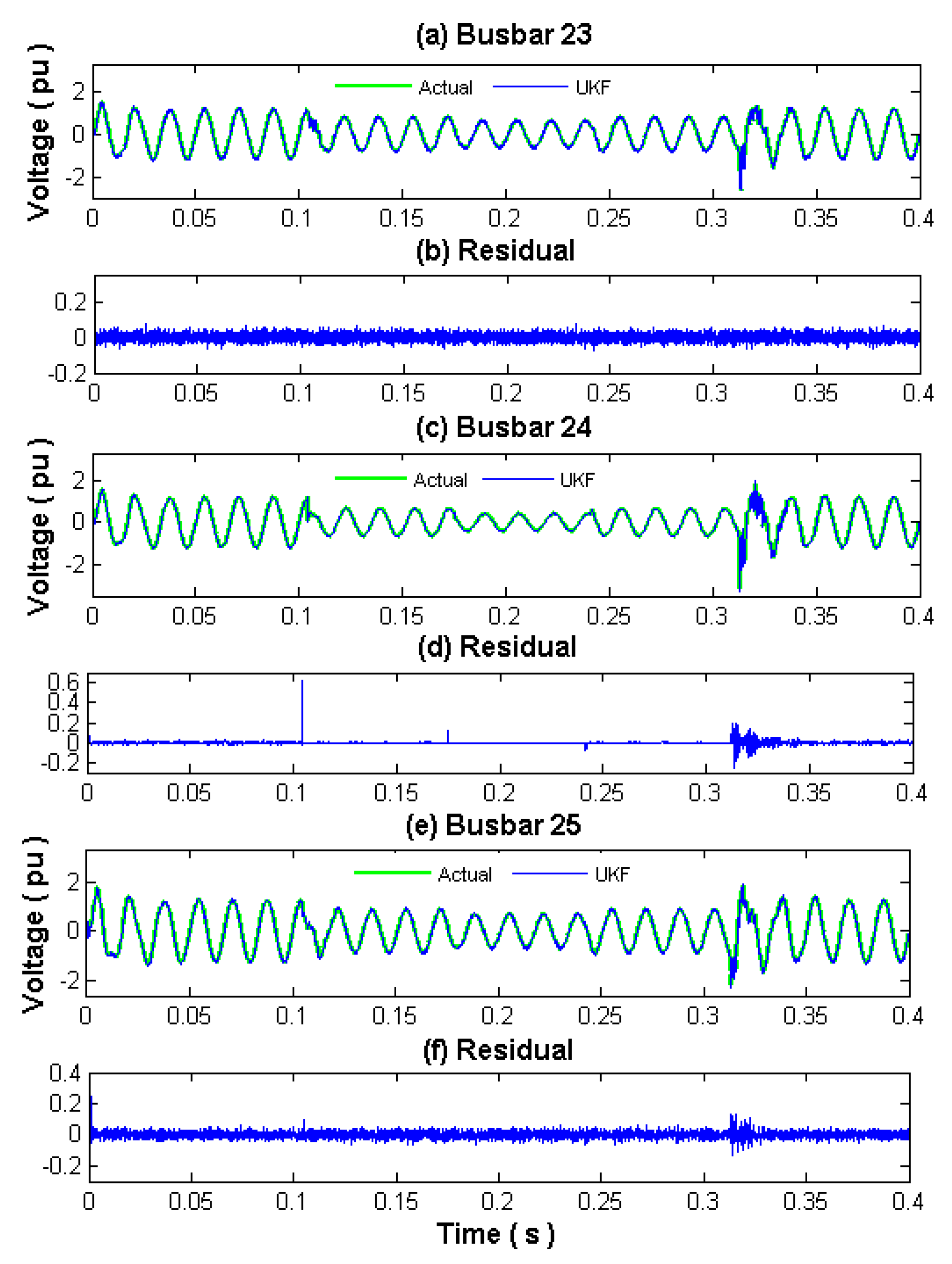
Figure 10 shows the voltage waveforms at busbars 23, 24, and 25 during the transient load condition. The busbar voltages show the largest fluctuations as a result of the varying load at busbar 24. When the load current increases 3 times, the busbar voltages tend to drop generating a voltage sag. The voltage drops during the first 4.25 cycles of the transient period (6.25 to 10.5 cycles) then again decreases over the next 4 cycles to show the effect of the load current, which increases 6 times during those 4 cycles (10.5 to 14.5 cycles). Finally, the current goes back to three times of the value at the initial period (14.5 to 18.75 cycles).
Load transient initiates at 6.25 cycles instead of 6 cycles to evaluate a more critical transient; similarly, the load transient finishes at 18.75 cycles instead of 18 cycles.
The transient state lasts 12.5 cycles (0.208 s), ending at 18.75 cycles (0.312 s), a voltage swell condition is present during the three cycles of the final transient period; voltage waveforms eventually reach the steady state close to the pre-fault operating condition.
NRMSE between actual and UKF estimated waveforms for voltage at busbars 23, 24 and 25 in Figure 10, are 0.45%, 0.40% and 2.43%, respectively.
The rms voltage magnitudes have been calculated using (26) for actual and UKF estimated waveforms during the transient load condition. Figure 11 shows the rms voltage magnitude for each cycle at busbars 21–26, which are close to the load transient of busbar 24.
The obtained rms voltage magnitudes represent the initial, transient and final operation periods, as well as the intermediate transient generating a fluctuating voltage sag. Actual and UKF estimate rms magnitudes closely agree. Please notice the voltage swell of different magnitude during the final period. The proposed UKF VSSE methodology closely estimates these voltage variations.
The use of detailed models to represent the power system components can reduce the state estimation error. Parameters should be close to their real values, filtering the noise from measurements before the assessment of the estimation, and increasing the available measurements.
It should be noted from the above case studies, that the UKF implemented in Matlab script language is still slow to be used in real-time applications. However, with adequate computational techniques such as parallel processing, better computational capability and programs compilation, the execution time can be significantly reduced.
5. Conclusions
A time-domain state estimation methodology for voltage sags in power networks using the UKF has been proposed. Nonlinear models for system and measurement equation have been used. It has been demonstrated that the UKF can be applied to precisely assess the voltage sag state estimation in power systems with nonlinear components. The proposed method has been verified using a modified version of the IEEE 30-bus test power system and noisy measurements.
It has been shown that the proposed UKF method dynamically follows the generation of voltage sags, by executing the estimator continuously, to record the voltage sags originated during the power network operation, especially for unmonitored busbars. This requires of an accurate model, a set of synchronized measurements preferably with low noise, sufficient to obtain an observable condition of busbar voltages. The measurement sampling frequency should satisfy the sampling theorem. The rms value can be computed from discrete waveforms; this value gives the information to define the sag magnitude, delimiting the sag time interval.
From the conducted case studies, it has been observed that when the power system goes under fast transients, the UKF estimator error is more noticeable; however, as the network evolves to steady state, the error quickly decreases to negligible proportions, i.e., on average 1%. In most cases, this period is short compared with the voltage sag estimation interval. This condition is present during the final period of the reviewed case studies, when the fault or transient condition is removed. It should be noted that usually at this time, a voltage swell is generated.
The state estimation error increases when sudden transient variations are present. The results obtained with the proposed UKF VSSE methodology have been successfully compared against actual values taken from a simulation of the test power system under the same transient condition. A close agreement has been achieved in all cases between the compared responses.
Author Contributions
R.C.-M. performed the simulation and modelling, analyzed the data, and wrote the paper. A.M. analyzed the results, reviewed the modeling and text, and supervised the related research work. O.A.-L. provided critical comments and revised the paper.
Acknowledgments
The authors gratefully acknowledge the Universidad Michoacana de San Nicolás de Hidalgo through the Facultad de Ingeniería Eléctrica, División de Estudios de Posgrado (FIE-DEP) Morelia, México, for the facilities granted to carry out this investigation. First two authors acknowledge financial assistance from CONACYT to conduct this investigation.
Conflicts of Interest
The authors declare no conflict of interest.
Nomenclature
| List of Abbreviations | |
| EAF | Electric arc furnace |
| FACTS | Flexible alternating current transmission system |
| KF | Kalman filter |
| NRMSE | Normalized root mean square error |
| PQ | Power quality |
| SNR | Signal to noise ratio |
| STATCOM | Static synchronous compensator |
| TCR | Thyristor-controlled rectifier |
| UKF | Unscented Kalman filter |
| UT | Unscented transform |
| VSSE | Voltage sags state estimation |
| WAMS | Wide area measurement system |
| List of Symbols | |
| e | State estimation error vector |
| f | Nonlinear state function |
| h | Nonlinear output function |
| k | Time instant t = k∆t |
| k + 1 | Time instant t = (k + 1)∆t |
| m | Number of measurements |
| n | Number of state variables |
| t | Time vector |
| u | Input vector |
| v | Process noise vector |
| w | Measurement noise vector |
| x | State vector |
| Estimated state vector | |
| y | Output vector |
| z | Measurement vector |
| E | Expected value |
| H | Measurements matrix |
| K | Kalman filter gain matrix |
| N | Normal distribution |
| P | Error covariance matrix |
| Q | Process noise covariance matrix |
| R | Measurement noise covariance matrix |
| Vrms | Rms voltage magnitude |
| W | Scalar weights |
| + | A posteriori or after measurement estimate |
| – | A priori or before measurement estimate |
| ∆t | Step time |
| α | Parameter to determine the spread of sigma points |
| β | Parameter to determine the distribution of x |
| λ | Scaling parameter |
| γ | Scaling parameter |
| κ | Parameter to determine the spread of sigma points |
| Sigma points matrix | |
Appendix A. Per Unit Additional Nonlinear Load Parameters
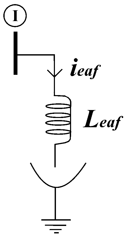
EAF busbar 2: Leaf = 0.5, k1 = 0.004, k2 = 0.0005, k3 = 0.005, m = 0, n = 2.0, initial condition EAF arc radius = 0.1
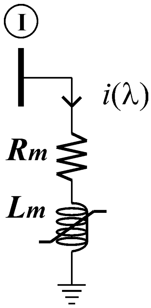
Nonlinear inductance busbar 5: Rm = 4.0, Lm = 1.0, n = 5.0, a = 0, b = 0.3
TCR busbar 6: Rtcr = 1.0, Ltcr = 0.5, firing angle α = 100 deg.
Appendix B. Nonlinear Models
Appendix B.1. Nonlinear Inductor
Figure A1 shows a nonlinear inductor.
Figure A1.
Nonlinear inductance.

According to KVL, the first-order differential equation to represent the nonlinear inductance is:
The discrete form of (A1) to define (8) and (9) is given by,
where Δt is the time step and k indicates the evaluation at time t(k).
The nonlinear solution of (A1), is represented by i(λ), λ is the nonlinear inductor magnetic flux, the polynomial approximation for i(λ) is:
n is an odd number due to the odd symmetry of (A3). Coefficients a, b and n adjust the nonlinear saturation curve. The rational fractions and hyperbolic approximations are alternative methods to represent this nonlinearity [38,39].
Appendix B.2. Electric Arc Furnace
Figure A2 shows the EAF model which can be expressed mathematically by two first-order nonlinear differential equations based on the energy conservation law, where the state variables are the arc radius reaf and the EAF current ieaf [39].
Figure A2.
Electric arc furnace.

The first-order nonlinear differential equations to represent the EAF are:
where n represents the arc cooling effect and m the arc column resistivity [38,39].
The following expressions give the discrete forms of (A4) and (A5) to define (8–9),
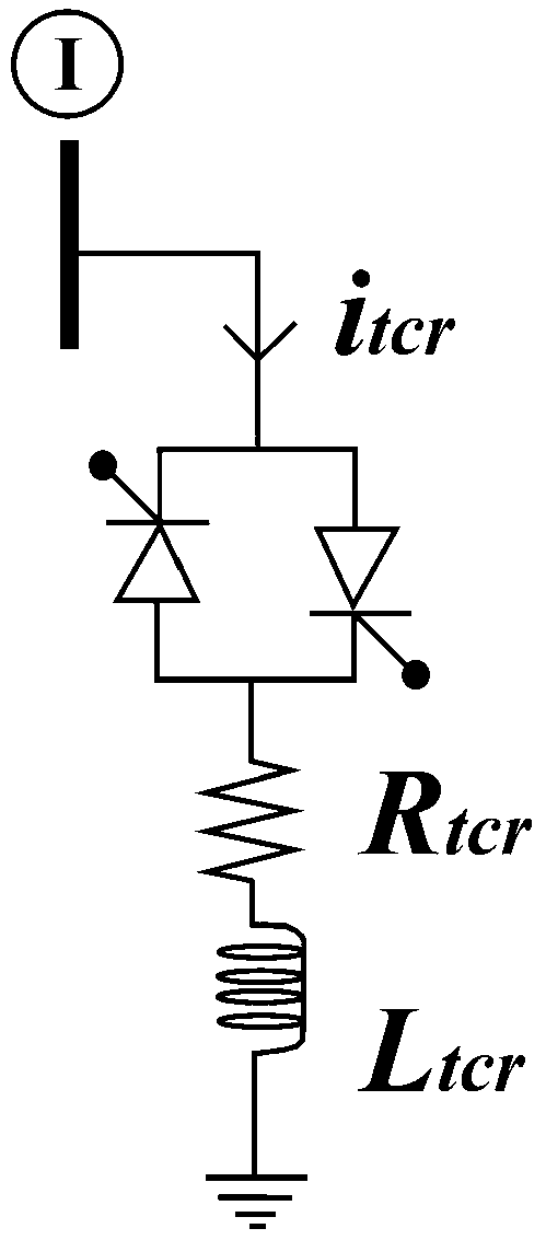
Appendix B.3. Thyristor Controlled Reactor
A thyristor pair back-to-back connection represents the TCR jointly with an RL circuit. The TCR current is the state variable, the TCR model is shown in Figure A3.
Figure A3.
Thyristor controlled reactor.

According to KVL, the first-order nonlinear differential equation modelling the TCR is:
The discrete form of (A8) to define (8) and (9) is given by,
The TCR current is controlled by the thyristor-firing angle α, the variable s represents this dependency being the switching function to turn on the thyristors, which varies according to the desired firing angle α. This generates harmonic distortion in the voltage and current waveforms. Because of this distortion, the TCR can be considered as a nonlinear component.
References
- Smith, J.C.; Hensley, G.; Ray, L. IEEE Recommended Practice for Monitoring Electric Power Quality; IEEE: Piscataway Township, NJ, USA, 1995; pp. 1159–1995. [Google Scholar]
- International Electrotechnical Commission (IEC). Int. Std. IEC 61000-4-30: Electromagnetic Compatibility (EMC) Part 4-30: Testing and Measurement Techniques—Power Quality Measurement Methods, 1st ed.; IEC: Geneva, Switzerland, 2003. [Google Scholar]
- IEEE Standard. IEEE Recommended Practice for Evaluating Electric Power System Compatibility with Electronic Process Equipment; IEEE: Piscataway Township, NJ, USA, 1998; pp. 1346–1998. [Google Scholar]
- National Electrical Manufacturers Association. American National Standard for Electric Power Systems and Equipment-Voltage Ratings (60 Hertz); C84.1-2011; National Electrical Manufacturers Association: Washington, DC, USA, 2011. [Google Scholar]
- Heydt, G.T. Electric Power Quality, 2nd ed.; Stars in a Circle Publications; Lafayette: Paris, France, 1991. [Google Scholar]
- Dugan, R.C.; Mcgranaghan, M.F.; Santoso, S.; Wayne, B.H. Electrical Power Systems Quality, 2nd ed.; McGraw-Hill: New York, NY, USA, 2002. [Google Scholar]
- Sankaran, C. Power Quality; CRC Press: Boca Raton, FL, USA, 2002. [Google Scholar]
- Bollen, M.H.J. Understanding Power Quality Problems Voltage Sags and Interruptions; IEEE Press Series on Power Engineering; IEEE: Piscataway Township, NJ, USA, 2000. [Google Scholar]
- Arrillaga, J.; Watson, N.R.; Chen, S. Power System Quality Assessment; John Wiley & Sons: Hoboken, NJ, USA, 2000. [Google Scholar]
- Watson, N.R. Power quality state estimation. Eur. Trans. Electr. Power 2010, 20, 19–33. [Google Scholar] [CrossRef]
- Yu, K.K.C.; Watson, N.R. An approximate method for transient state estimation. IEEE Trans. Power Deliv. 2007, 22, 1680–1687. [Google Scholar] [CrossRef]
- Medina, A.; Cisneros-Magaña, R. Time-domain harmonic state estimation based on the Kalman filter Poincaré map and extrapolation to the limit cycle. IET Gener. Transm. Distrib. 2012, 6, 1209–1217. [Google Scholar] [CrossRef]
- Cisneros-Magaña, R.; Medina, A. Time domain transient state estimation using singular value decomposition Poincare map and extrapolation to the limit cycle. Electr. Power Energy Syst. 2013, 53, 810–817. [Google Scholar] [CrossRef]
- Espinosa-Juarez, E.; Hernandez, A. A method for voltage sag state estimation in power systems. IEEE Trans. Power Deliv. 2007, 22, 2517–2526. [Google Scholar] [CrossRef]
- Mallick, R.K. Application of linear Kalman filter in power quality estimation. In Proceedings of the ITR International Conference, Bhubaneswar, India, 6 April 2014; ISBN 978-93-84209-02-5. [Google Scholar]
- Cisneros-Magaña, R.; Medina, A.; Segundo-Ramírez, J. Efficient time domain power quality state estimation using the enhanced numerical differentiation Newton type method. Electr. Power Energy Syst. 2014, 63, 141–422. [Google Scholar] [CrossRef]
- Siavashi, E.M.; Rouhani, A.; Moslemi, R. Detection of voltage sag using unscented Kalman smoother. In Proceedings of the 2010 9th International Conference on Environment and Electrical Engineering (EEEIC), Prague, Czech Republic, 16–19 May 2010; Volume 1, pp. 128–131. [Google Scholar] [CrossRef]
- Kusko, A.; Thompson, M.T. Power Quality in Electrical Systems; McGraw-Hill: New York, NY, USA, 2007. [Google Scholar]
- Fuchs, E.F.; Masoum, M.A.S. Power Quality in Power Systems and Electrical Machines; Academic Press Elsevier: New York, NY, USA, 2008. [Google Scholar]
- Baggini, A. Handbook of Power Quality; John Wiley & Sons: Hoboken, NJ, USA, 2008. [Google Scholar]
- Shahriar, M.S.; Habiballah, I.O.; Hussein, H. Optimization of Phasor Measurement Unit (PMU) Placement in Supervisory Control and Data Acquisition (SCADA)-Based Power System for Better State-Estimation Performance. Energies 2018, 11, 570. [Google Scholar] [CrossRef]
- Moreno, V.M.; Pigazo, A. Kalman Filter: Recent Advances and Applications; I-Tech Education and Publishing: Vienna, Austria, 2009. [Google Scholar]
- Chen, R.; Lin, T.; Bi, R.; Xu, X. Novel Strategy for Accurate Locating of Voltage Sag Sources in Smart Distribution Networks with Inverter-Interfaced Distributed Generators. Energies 2017, 10, 1885. [Google Scholar] [CrossRef]
- Amit, J.; Shivakumar, N.R. Power system tracking and dynamic state estimation. Power Syst. Conf. Exp. 2009. [Google Scholar] [CrossRef]
- Wang, S.; Gao, W.; Meliopoulos, A.P.S. An alternative method for power system dynamic state estimation based on unscented transform. IEEE Trans. Power Syst. 2012, 27, 942–950. [Google Scholar] [CrossRef]
- Charalampidis, A.C.; Papavassilopoulos, G.P. Development and numerical investigation of new non-linear Kalman filter variants. IET Control Theory Appl. 2011, 5, 1155–1166. [Google Scholar] [CrossRef]
- Tebianian, H.; Jeyasurya, B. Dynamic state estimation in power systems: Modeling, and challenges. Electr. Power Syst. Res. 2015, 121, 109–114. [Google Scholar] [CrossRef]
- Lalami, A.; Wamkeue, R.; Kamwa, I.; Saad, M.; Beaudoin, J.J. Unscented Kalman filter for non-linear estimation of induction machine parameters. IET Electr. Power Appl. 2012, 6, 611–620. [Google Scholar] [CrossRef]
- Ghahremani, E.; Kamwa, I. Online state estimation of a synchronous generator using unscented Kalman filter from phasor measurements units. IEEE Trans. Energy Convers. 2011, 26, 1099–1108. [Google Scholar] [CrossRef]
- Julier, S.J.; Uhlmann, J.K. Unscented filtering and nonlinear estimation. Proc. IEEE 2004, 92, 401–422. [Google Scholar] [CrossRef]
- Qing, X.; Yang, F.; Wang, X. Extended set-membership filter for power system dynamic state estimation. Electr. Power Syst. Res. 2013, 99, 56–63. [Google Scholar] [CrossRef]
- Huang, M.; Li, W.; Yan, W. Estimating parameters of synchronous generators using square-root unscented Kalman filter. Electr. Power Syst. Res. 2010, 80, 1137–1144. [Google Scholar] [CrossRef]
- Van der Merwe, R.; Wan, E.A. The square-root unscented Kalman filter for state and parameter estimation. In Proceedings of the 2001 IEEE International Conference on Acoustics, Speech, and Signal Processing, Salt Lake City, UT, USA, 7–11 May 2001. [Google Scholar]
- Aghamolki, H.G.; Miao, Z.; Fan, L.; Jiang, W.; Manjure, D. Identification of synchronous generator model with frequency control using unscented Kalman filter. Electr. Power Syst. Res. 2015, 126, 45–55. [Google Scholar] [CrossRef]
- Bretas, N.; Bretas, A.; Piereti, S. Innovation concept for measurement gross error detection and identification in power system state estimation. IET Gener. Transm. Distrib. 2011, 5, 603–608. [Google Scholar] [CrossRef]
- Jain, S.K.; Singh, S.N. Harmonics estimation in emerging power system: Key issues and challenges. Electr. Power Syst. Res. 2011, 81, 1754–1766. [Google Scholar] [CrossRef]
- University of Washington, Electrical Engineering, Power Systems Test Case Archive. Available online: http://www.ee.washington.edu/research/pstca/pf30/pg_tca30bus.htm (accessed on 15 March 2018).
- Waston, N.R.; Bathurst, G. Task Force on Harmonics Modeling and Simulation, Modeling devices with nonlinear voltage-current characteristics for harmonic studies. IEEE Trans. Power Deliv. 2004, 19, 1802–1811. [Google Scholar] [CrossRef]
- Acha, E.; Madrigal, M. Power Systems Harmonics Computer Modelling and Analysis; John Wiley & Sons: Hoboken, NJ, USA, 2001. [Google Scholar]
Figure 1.
Time-domain UKF VSSE.

Figure 2.
Modified IEEE 30-bus test power system with nonlinear loads at busbars 2, 5, and 6.

Figure 3.
Busbar voltages (a) Actual, (b) UKF VSSE, (c) Difference, short-circuit at busbar 4 from 0.216 to 0.283 s.
Figure 3.
Busbar voltages (a) Actual, (b) UKF VSSE, (c) Difference, short-circuit at busbar 4 from 0.216 to 0.283 s.

Figure 4.
Actual, UKF estimation, and residuals of busbars 4 and 6, voltage sag 14–17 cycles from 0.216 to 0.283 s, voltage swell 18–19 cycles, short-circuit at busbar 4.
Figure 4.
Actual, UKF estimation, and residuals of busbars 4 and 6, voltage sag 14–17 cycles from 0.216 to 0.283 s, voltage swell 18–19 cycles, short-circuit at busbar 4.

Figure 5.
Line currents (a) Actual, (b) UKF estimation, (c) Difference, short-circuit at busbar 4 from 0.216 to 0.283 s.
Figure 5.
Line currents (a) Actual, (b) UKF estimation, (c) Difference, short-circuit at busbar 4 from 0.216 to 0.283 s.

Figure 6.
Nonlinear load currents, actual, UKF, and residuals, short-circuit at busbar 4 from 0.216 to 0.283 s.
Figure 6.
Nonlinear load currents, actual, UKF, and residuals, short-circuit at busbar 4 from 0.216 to 0.283 s.

Figure 7.
Actual, UKF VSSE, rms voltage magnitude for faulted busbar 4 and busbars 3, 6, 9, 12, and 14. Sags of different magnitude are present from 0.216 to 0.283 s. Swells are present at first post-fault cycle after 0.283 s.
Figure 7.
Actual, UKF VSSE, rms voltage magnitude for faulted busbar 4 and busbars 3, 6, 9, 12, and 14. Sags of different magnitude are present from 0.216 to 0.283 s. Swells are present at first post-fault cycle after 0.283 s.

Figure 8.
Actual and UKF estimated voltage waveforms of busbars 15 and 23, voltage sag from 0.216 to 0.283 s, cycles 14–17, voltage swell during cycle 18, short-circuit at busbar 15.
Figure 8.
Actual and UKF estimated voltage waveforms of busbars 15 and 23, voltage sag from 0.216 to 0.283 s, cycles 14–17, voltage swell during cycle 18, short-circuit at busbar 15.

Figure 9.
Actual and UKF rms voltage, short-circuit at busbar 15 during 14–17 cycles, from 0.216 to 0.283 s.
Figure 9.
Actual and UKF rms voltage, short-circuit at busbar 15 during 14–17 cycles, from 0.216 to 0.283 s.

Figure 10.
Voltage waveforms, actual, UKF, and residuals of busbars 23, 24, and 25; transient load condition at busbar 24 (0.104 to 0.312 s).
Figure 10.
Voltage waveforms, actual, UKF, and residuals of busbars 23, 24, and 25; transient load condition at busbar 24 (0.104 to 0.312 s).

Figure 11.
Actual and UKF rms voltage magnitudes, transient load condition at busbar 24 from 0.104 to 0.312 s, during 6.25–18.75 cycles.
Figure 11.
Actual and UKF rms voltage magnitudes, transient load condition at busbar 24 from 0.104 to 0.312 s, during 6.25–18.75 cycles.


Table 1.
State variable vector x.
| Description | State Variable |
|---|---|
| Line currents | 1–41 |
| Busbar voltages | 42–71 |
| Generator currents | 72–77 |
| Busbar load currents | 78–106 |
| Nonlinear inductor magnetic flux | 107 |
| EAF current and arc radius | 108–109 |
| TCR current | 110 |
Table 2.
Measurements vector z.
| Description | Output Variable |
|---|---|
| Line currents | 1–38 |
| Busbar voltages | 42–68 |
| Generator currents | 72–77 |
| Busbar load currents | 78–106 |
| Nonlinear inductor current | 107 |
| EAF real power | 108–109 |
Table 3.
Actual and UKF VSSE voltage sags (pu).
| Busbar | Actual | UKF | Busbar | Actual | UKF |
|---|---|---|---|---|---|
| 3 | 0.752 | 0.753 | 19 | 0.889 | 0.890 |
| 4 | 0.713 | 0.717 | 20 | 0.889 | 0.890 |
| 6 | 0.858 | 0.860 | 21 | 0.892 | 0.892 |
| 7 | 0.908 | 0.910 | 22 | 0.892 | 0.893 |
| 9 | 0.870 | 0.876 | 23 | 0.893 | 0.893 |
| 10 | 0.890 | 0.900 | 24 | 0.887 | 0.888 |
| 12 | 0.870 | 0.880 | 25 | 0.888 | 0.889 |
| 14 | 0.880 | 0.885 | 26 | 0.892 | 0.892 |
| 15 | 0.872 | 0.873 | 27 | 0.891 | 0.892 |
| 16 | 0.880 | 0.890 | 28 | 0.880 | 0.881 |
| 17 | 0.892 | 0.895 | 29 | 0.884 | 0.885 |
| 18 | 0.875 | 0.880 | 30 | 0.907 | 0.909 |
Table 4.
Transient load condition.
| Period | Cycles | Time (s) | Load Current (pu) |
|---|---|---|---|
| Initial | 00.00–06.25 | 0.000–0.104 | 1.00 |
| Load transient 1 | 06.25–10.50 | 0.104–0.175 | 3.00 |
| Load transient 2 | 10.50–14.50 | 0.175–0.241 | 6.00 |
| Load transient 3 | 14.50–18.75 | 0.241–0.312 | 3.00 |
| Final | 18.75–24.00 | 0.312–0.400 | 1.00 |
© 2018 by the authors. Licensee MDPI, Basel, Switzerland. This article is an open access article distributed under the terms and conditions of the Creative Commons Attribution (CC BY) license (http://creativecommons.org/licenses/by/4.0/).
Share and Cite
MDPI and ACS Style
Cisneros-Magaña, R.; Medina, A.; Anaya-Lara, O. Time-Domain Voltage Sag State Estimation Based on the Unscented Kalman Filter for Power Systems with Nonlinear Components. Energies 2018, 11, 1411. https://doi.org/10.3390/en11061411
AMA Style
Cisneros-Magaña R, Medina A, Anaya-Lara O. Time-Domain Voltage Sag State Estimation Based on the Unscented Kalman Filter for Power Systems with Nonlinear Components. Energies. 2018; 11(6):1411. https://doi.org/10.3390/en11061411
Chicago/Turabian StyleCisneros-Magaña, Rafael, Aurelio Medina, and Olimpo Anaya-Lara. 2018. "Time-Domain Voltage Sag State Estimation Based on the Unscented Kalman Filter for Power Systems with Nonlinear Components" Energies 11, no. 6: 1411. https://doi.org/10.3390/en11061411
Note that from the first issue of 2016, this journal uses article numbers instead of page numbers. See further details here.