Improved Genetic Algorithm-Based Unit Commitment Considering Uncertainty Integration Method

Department of Energy System Engineering, Chung-Ang University, 84 Heukseok-ro, Dongjak-gu, Seoul 06974, Korea
*
Author to whom correspondence should be addressed.
Energies 2018, 11(6), 1387; https://doi.org/10.3390/en11061387
Submission received: 3 May 2018
/
Revised: 24 May 2018
/
Accepted: 28 May 2018
/
Published: 29 May 2018
(This article belongs to the Special Issue Electric Power Systems Research 2018)
Abstract
:In light of the dissemination of renewable energy connected to the power grid, it has become necessary to consider the uncertainty in the generation of renewable energy as a unit commitment (UC) problem. A methodology for solving the UC problem is presented by considering various uncertainties, which are assumed to have a normal distribution, by using a Monte Carlo simulation. Based on the constructed scenarios for load, wind, solar, and generator outages, a combination of scenarios is found that meets the reserve requirement to secure the power balance of the power grid. In those scenarios, the uncertainty integration method (UIM) identifies the best combination by minimizing the additional reserve requirements caused by the uncertainty of power sources. An integration process for uncertainties is formulated for stochastic unit commitment (SUC) problems and optimized by the improved genetic algorithm (IGA). The IGA is composed of five procedures and finds the optimal combination of unit status at the scheduled time, based on the determined source data. According to the number of unit systems, the IGA demonstrates better performance than the other optimization methods by applying reserve repairing and an approximation process. To account for the result of the proposed method, various UC strategies are tested with a modified 24-h UC test system and compared.
1. Introduction
Global environmental problems are becoming a major issue in the power industry. Recently, renewable energies such as wind and solar have become preferable, because they are economical and relatively less adverse to the environment [1]. However, these renewable sources possess intermittent characteristics, which may lead to significant unexpected loads and operational problems in power grid. Power system operations are designed to address a limited amount of uncertainty in the system, which does not consider changes due to the use of renewable energy at an unprecedented scale. When renewable energy is associated with power system operation, their characteristic problems appear larger [2]. To solve the intermittency problem, an accurate prediction of renewable sources that considers volatility is needed [3]. Therefore, it is necessary to develop a framework not only to consider the uncertainties of renewable energies, but also to improve the potential risks of the power grid.
The unit commitment (UC) problem is an optimization procedure that deducts the best combinations of units in on and off status, which is important for power system operational planning. Generally, the UC problem constitutes a process of calculating system operating cost by optimizing the schedule of the generating units such that the load of time-varying is secured by taking account of the constraints of system. In the existing power system, it has become difficult to determine the UC of various renewable sources that have been recently connected, and their intermittent nature makes it difficult to optimize the operation of the system. Thus, it is necessary to find a UC solution that considers the uncertainties of renewable energy and apply it to a framework to mitigate a risk caused by uncertainties.
Many studies have been conducted to optimize UC problems, such as memetic algorithms [4], bacterial foraging [5], second-order cone programming [6], mixed-integer programming [7], particle swarm optimization [8], discrete differential evolution method [9], and genetic algorithms (GA) [10]. Based on these optimization algorithms, progress with UC problems has also been made by considering the volatility, intermittency, and uncertainty of system constraints. A fuzzy mathematical programming model has been suggested to resolve the problem of unit scheduling for solar and wind energy [11]. This fuzzy optimization method was designed to acquire optimal unit scheduling through fuzzy sets and a membership function. A stochastic programming framework was implemented in ref. [12], which was built as a multi-objective problem. In this model, uncertainties of load, solar, wind, and market price are modeled, which is based on scenario stochastic programming. The interval optimization approach and a stochastic model for security-constrained UC were illustrated in ref. [13]. The approach is formed by a mixed-integer programming problem that is composed of two approaches: interval optimization solution and a scenario-based solution. In another study, a solution for a long-term security-constrained UC was described [14]. Scenario-based stochastic unit commitment (SUC), including a worst-case analysis, was described in ref. [15]. In this study, the management is conducted with a loss of the load risk by using the conditional value-at-risk. The proposed SUC problem is modeled in a mixed-integer linear programming formulation and solved by a modified Benders decomposition algorithm with two enhancement strategies. In ref. [16], a robust optimization was proposed that is based on the outer approximation technique and Benders decomposition algorithm. In ref. [17], the authors introduced a UC solution that was based on the robust optimization that accounted for the fluctuation scenario of the worst wind power. Recently, a profit-based UC problem was solved through a hybrid optimization technique [18]. The technique is based on the integration of binary successive approximation. In ref. [19], authors addressed the design of a convex model that is based on conic relaxations with valid inequalities. To improve forecast accuracy, the authors suggested a method that includes temperature variables from two thermal regions [20]. Short-term forecasting and UC are combined and formulated in the model. In ref. [21], a technique to resolve the UC problem based on an imperialistic competition algorithm has been described by using cluster algorithm. However, most of the models focused only on stochastic methods modeling, which did not consider the correlation of uncertainties. Moreover, there was no extensive comparative study of deterministic and stochastic UC solutions.
In this paper, an improved genetic algorithm (IGA)-based procedure is proposed to resolve the UC problem. Uncertainties in wind power, solar power, and load are represented with a normal distribution in a Monte Carlo simulation. The value of generator outages is given by a capacity outage probability table. Within the range of reserve requirements to be secured, the best combination of scenarios for load, wind, and solar is assembled by using the uncertainty integration method (UIM). Based on the UIM, the stochastic unit commitment (SUC) problem is formulated with non-linear optimization under various thermal unit constraints by using IGA, which consists of five processes. In particular, a modified repair operator and an approximation process make IGA efficient. The result of the UC problem with deterministic cases using IGA compared with other optimization methods demonstrates the algorithm’s effectiveness.
The remainder of this paper is arranged as follows. The structure of the UIM is illustrated in Section 2. Section 3 presents a mathematical formulation that take into account system constraints. The IGA-based UC procedure is described in Section 4. The results of numerical studies are provided in Section 5, along with an analysis of the computational time, reserve requirements, and operating costs. The conclusions are given in Section 6.
2. Uncertainty Integration Method
2.1. Uncertainty Modeling
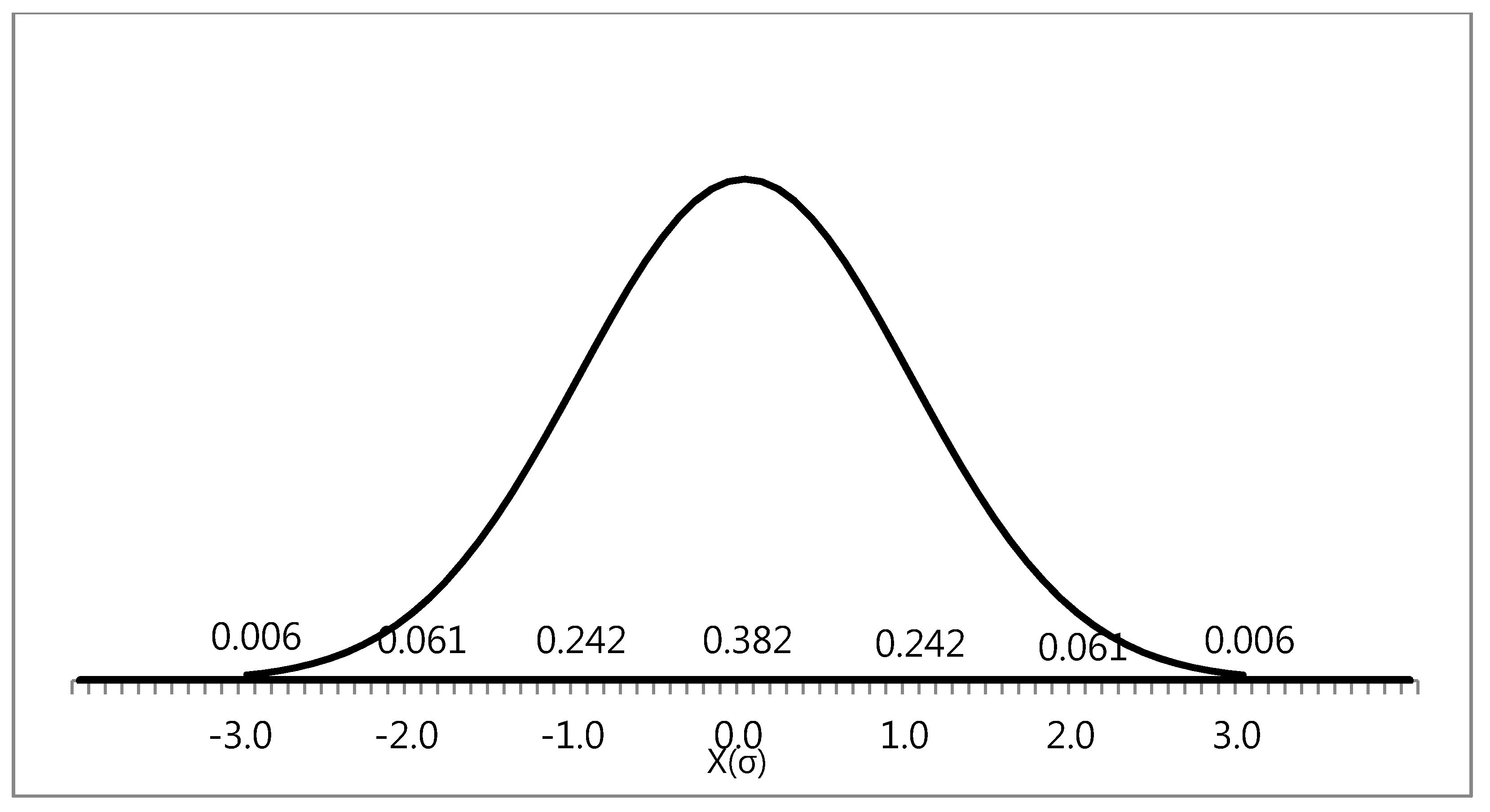
In the UC problem, the forecasting of uncertainty is a key factor, because it is needed to protect the power system from a sudden load increase. It also has an effect on calculations of the operating cost and planning for the reserve requirement. Thus, to guarantee the economical operation and reliability of the power grid, it is necessary to accurately predict uncertainty. Uncertainty in load forecasting could be reasonably illustrated by a normal distribution that can be estimated from past experience and future considerations. The uncertainty of load forecasting is expressed as a probability distribution where the predicted peak load is expressed with a distribution mean and standard deviation. The probability distribution can be divided into a discrete number of class intervals. The area of each class interval represents the probability of the load, which is equal to the class interval mid-value. The mean absolute percentage error is used as a basis for calculating the range of forecasting errors, and the range is set from 2% to 4% for day-ahead load forecasting [22].
Generally, renewable energy is a fluctuating and uncontrollable power source. For this reason, forecasting errors should be accurately measured when solving the UC problem. The active power of wind is expressed as a function of the wind speed constant rated power between the rated wind speed and the cutout wind speed. It is described in Equations (1)–(3).
The active power of solar energy is expressed by the power density, ambient temperature at the solar plant, and solar irradiation. It is represented in Equation (4).
To obtain accurate predictions, the normal distribution is used as the joint probability density function of short-term solar power and wind power output [23]. At each time interval, the expected value of output from the renewable sources is selected as the mean value. The standard deviation is then determined by a specific percentage of the mean value, and it depends on the level of forecasting error. Based on this value, a large number of random computational scenarios are generated by Monte Carlo simulation. Uncertainties distribution is shown in Figure 1.
In this study, generator outages are also considered to have a discrete probability distribution and are shown in a probability table of a capacity outage [24]. The table provides the probability of occurrence in each capacity of generator outage. To make the UIM simpler and ensure compatibility by using the concept of net load, a similar generator can be applied to express the generator outage’s uncertainty. If the generator has sudden outages, a scenario is created with the same demand growth, and demand increases will happen during the period in which the generator is assumed to have an outage. In our work, the outage rate of the expected forced generator is 2%. Duration and the outage rate can be conformed according to the historical outage statistics for different generators.
2.2. Scenario Integration Technique
The process of scenario generation is to choose measurements and predict inputs, parameters, and disturbances to acquire the best solution. This process is used to resolve problems related to uncertainty constraints with a normal distribution, and a probability distribution based on Monte Carlo simulation. The value of uncertainty prediction for each of the wind, solar, load, and generator outages is calculated through scenario generation. These uncertainties are integrated through the scenario integration technique, which is the process of computing values by calculating the association between uncertainties that occur as a result of considering various sources in the power grid. The values of load, wind power, and solar power, including the predictions for each uncertainty, are selected to determine the best scenario to meet the reserve needs. The process of uncertainty integration is as follows.
Forecasting errors of the load, solar power, and wind power are represented in Equations (5)–(7).
The prediction error of the energy sources meets the constraints using a spinning reserve of the thermal unit. The reserve requirement considering the forecasting error constraint of the energy source is expressed by Equations (8) and (9).
To compensate for unpredicted fluctuation in energy sources, an additional reserve requirement is estimated to be a percentage of the load in the power grid. Accordingly, the additional reserve requirements are reformulated as Equations (10)–(12).
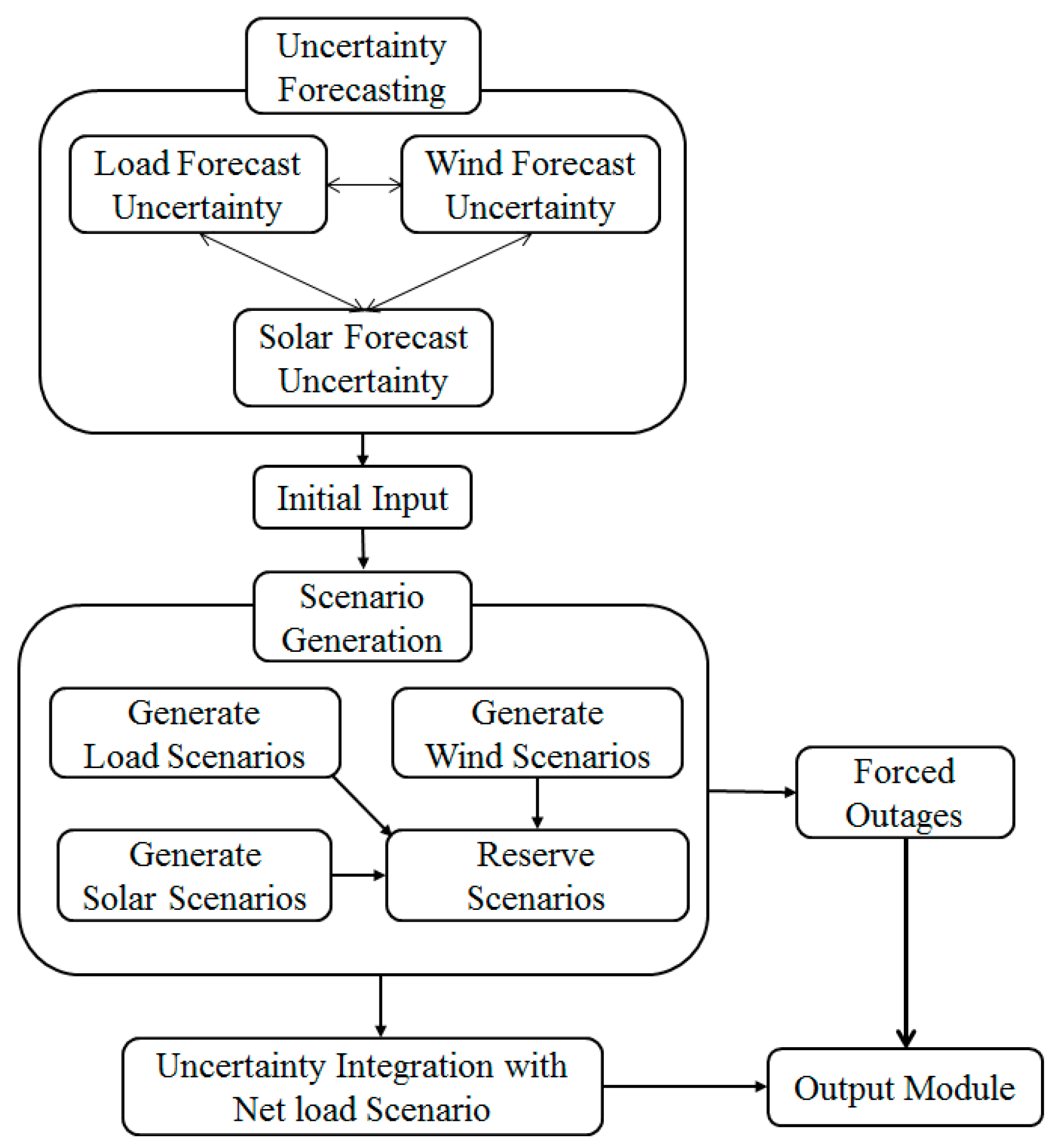
The net load concept simplified the formulation of the UC problem. Due to the intermittency of the energy sources, it is necessary to predetermine a schedule that meets the net load. Based on the predicted values, hourly random loads, solar power, and wind power are considered in each scenario. The probability of the scenario determines the value of each parameter, and the realization of future random processes is represented by each of these scenarios. Figure 2 shows the structure of UIM. A separate module or sub-module is represented by each function. The initial input data is calculated with the forecasted value for each hour for day-ahead scheduling. Using Monte Carlo simulation, a scenario is generated that considers forecasting error information. The output of the load, wind, and solar scenarios is used with the prediction error to calculate reserve scenarios. An additional reserve is calculated from the generator outages of a thermal generator. Uncertainties of the input energy sources are integrated through the net load concept, and a 24-h net load scenario is created.
3. Proposed Stochastic Unit Commitment Formulation
Generally, the current UC problems have been formulated with many additional operation constraints, namely emissions, transmission, and other services [25,26]. However, in this paper, we focused on the effects of uncertainties constraints, which do not consider emission, transmission constraints, and other services in this SUC model.
3.1. Objective Function
The objective function involves status of unit and power outputs for distributed power generators at each time in respective scenario. The purpose of the function is to minimize the operating cost. The objective function is described as Equation (13):
This function consists of three parts: start-up cost, shut-down cost, and the fuel cost of all of the thermal generators. The fuel cost of a thermal generator is generally represented by a quadratic function. Here, the operating costs of wind turbines and solar turbines are generally excluded when computing total operating costs.
The start-up cost and shut-down cost of the thermal unit is calculated by the following linear function.
3.2. System Constraints
The load for every combination to satisfy the constraints of the power balance should equal the total generated power over each time interval in each scenario. Power balance constraints are described as Equation (16).
In the power system, some amount of reserve is needed to complement unbalance between the load and the power output. It is shown in Equations (17)–(20).
An amount of spinning reserve should be prepared so that even if one unit is lost, the system frequency will not drop too much. The up-spinning reserve complements a sudden increase in load by ramping up the capacity of the unit when the load is suddenly increased.
3.3. Thermal Unit Constraints
The minimum and maximum power output limits must be satisfied in each thermal unit. It is represented by following formulation:
The minimum time limits of each unit’s on and off g are expressed as:
The power output of the thermal unit cannot be altered by more than a certain amount for time t of the optimization period. This is because sudden fluctuations in the power output of the generator can cause damage to the turbine. For each generator, the constraints of the operating ramp rate are formulated in Equations (24)and (25).
Constraints of the shut-down costs and start-up costs are represented in Equation (26):
4. IGA-Based SUC Problem Solution
4.1. Improved Genetic Algorithm
The SUC problem is a generally non-linear optimization problem under various constraints. However, in order to obtain a UC solution, a proposed SUC model is linearized and approximated in the formulation and optimization procedure. The problem is constructed by considering generation scheduling and inequality constraints on unit on/off states. The results of the optimal UC schedule should be economical and reliable. The results obtained in the deterministic UC may not be accurate due to the uncertainty of energy sources, whereas the stochastic model allows for a more accurate estimation of the variability of energy sources, which are considered with respect to each other through the UIM. To solve this problem, we propose an IGA-based solution that is a development of the conventional GA [10]. A GA is better suited to solving UC problems using binary representations than other methods for parameter optimization. However, conventional GAs only work efficiently in the optimization of objective functions without constraints. The binding constraints disturb the efficiency of the search process in a GA. Moreover, the existing GA has a problem in that the computational time is very long when the system size is large, as well as when it operates in a wide search space including infeasible solutions. On the other hand, the IGA offers some advantages compared with the standard GA. First, it does not work in a broad search space with infeasible solutions, but it does work with a feasible solution to reduce the search area. The IGA also consumes less computation, and thus, the best solution can be determined through the violation of constraints using a repair and approximation procedure. To provide a feasible solution to the problem, the constraints are formulated as penalty objective functions.
Therefore, in the IGA, this is accomplished through crossover, swap mutation, repair operators, approximation operators, and selection. The IGA offers economic efficiency and stability compared with the standard GA. The algorithm is implemented as shown below.
- (1)
- (2)
- Swap mutation: Figure 4 shows the swap mutation process, which is sorted in descending order in accordance with the operating cost of each generator. The probability of initial mutation is 0.2. Operating cost is obtained by considering the heat rate of the fuel cost at a full load time. If the average operating cost of the i-th unit is lower than that of the j-th unit, and the units are “ON” and “OFF”, respectively, the states of the i-th and j-th units are switched with each other. This procedure is performed for each scheduled time, which helps to lower the operating cost. The swap mutation process is shown in Figure 4.
- (3)
- Repairing: The repairing operator modifies an infeasible solution by considering the minimum-up and minimum-down constraints. The state of the generator is checked every time interval, and if the minimum-up and minimum-down time constraint is limited at a given time t, the state of the unit is reversed and updated at that time.
- (4)
- Approximation: This operator approximates an infeasible solution under conditions that satisfy demand and spinning reserve constraints. The demand and spinning reserve constraints are examined every hour to determine whether to change the state of the unit or not.
- (5)
- Selection: Entire units are displayed in descending order. The best solution is gained by considering fuel cost and various constraints. Maximum iteration value is 300.
4.2. Solution Procedure of Unit Commitment
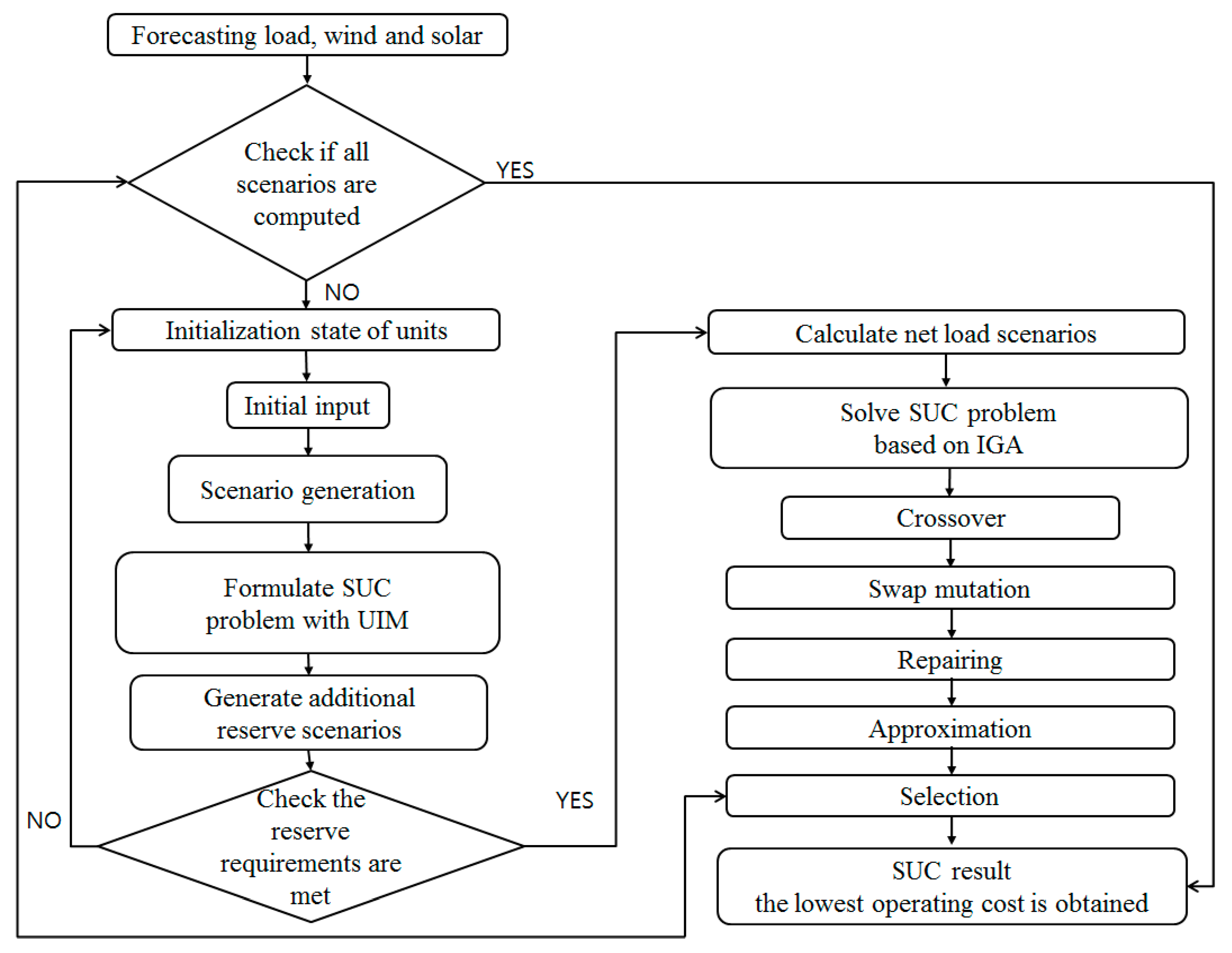
Figure 5 summarizes the proposed solution process for SUC problems. The procedure is implemented sequentially. Initial input data is calculated based on available system information and predictions. A scenario is generated by using Monte Carlo simulation, and the SUC problem is then formulated. After generating energy sources that take uncertainty into account, additional reserve requirements are calculated from Equations (10) and (11). In this process, we find the combination of scenarios for energy sources generated through UIM that best complement each other’s uncertainties. Here, the power system balance will be checked, including the reserve requirement. If the balance is not satisfied, the system goes back to the initial state, and restarts the first process again. The net load scenario is calculated by considering Equation (12). In this process, we find that several random scenarios obtain a better combination, and then the UC problem is optimized through IGA. This procedure makes repetition continuously to gain the best solution.
5. Simulation Results
5.1. Performance Comparison of Optimization Algorithm
To show the performance of IGA, IGA was compared with other optimization algorithms in the deterministic cases [28,29,30,31,32,33,34,35]. Power systems of 10, 20, 40, 60, 80, and 100 units with a planning horizon of 24 h are simulated in each test case. The base case is a 10-unit power system. The parameter and load demands of the base case during a 24-h cycle can be found in ref. [36]. Each power system is obtained by using the 10-unit base case, while the demands are altered in part of the size of the system. In our study, the spinning reserve is supposed to be 10% of the load demand. IGA is executed with 30 runs on each test case. For other parameters used in the IGA, the iteration number is 200. IGA is also implemented in MATLAB and simulated on a laptop computer with an Intel quad-core 3.20 GHz processor, 8 GB of memory, and a 64-bit Windows 7 operating system.
Table 1 represents a comparison of the operating costs of the schedules obtained by each algorithm. IGA presents the lowest operating cost over most power system sizes, except for the 10-unit test system, whereas LR (Lagrangian Relaxation) and ES-PSO (Expert System-Particle Swarm Optimization) offer the lowest operating cost in a 10-unit test system. In general, because the differences between the best and worst of each case could represent the algorithms’ robustness, large differences between cases means that the result of the algorithm’s optimization has high volatility, and it cannot guarantee a stable result. Comparing each test case, IGA provides better performance, because the difference between best and worst is smaller than with other algorithms. The operating costs of the UC calculated by IGA are smaller than those from PSO (Particle Swarm Optimization), IBPSO (Improved Binary Particle Swarm Optimization), QBPSO (Quantum-inspired binary Particle Swarm Optimization), and ES-PSO, especially for test cases of a large number of units. The results demonstrate that the reserve repairing and approximation process that commit/decommit units for a successive period of hours can improve the efficiency and lower the operating cost.
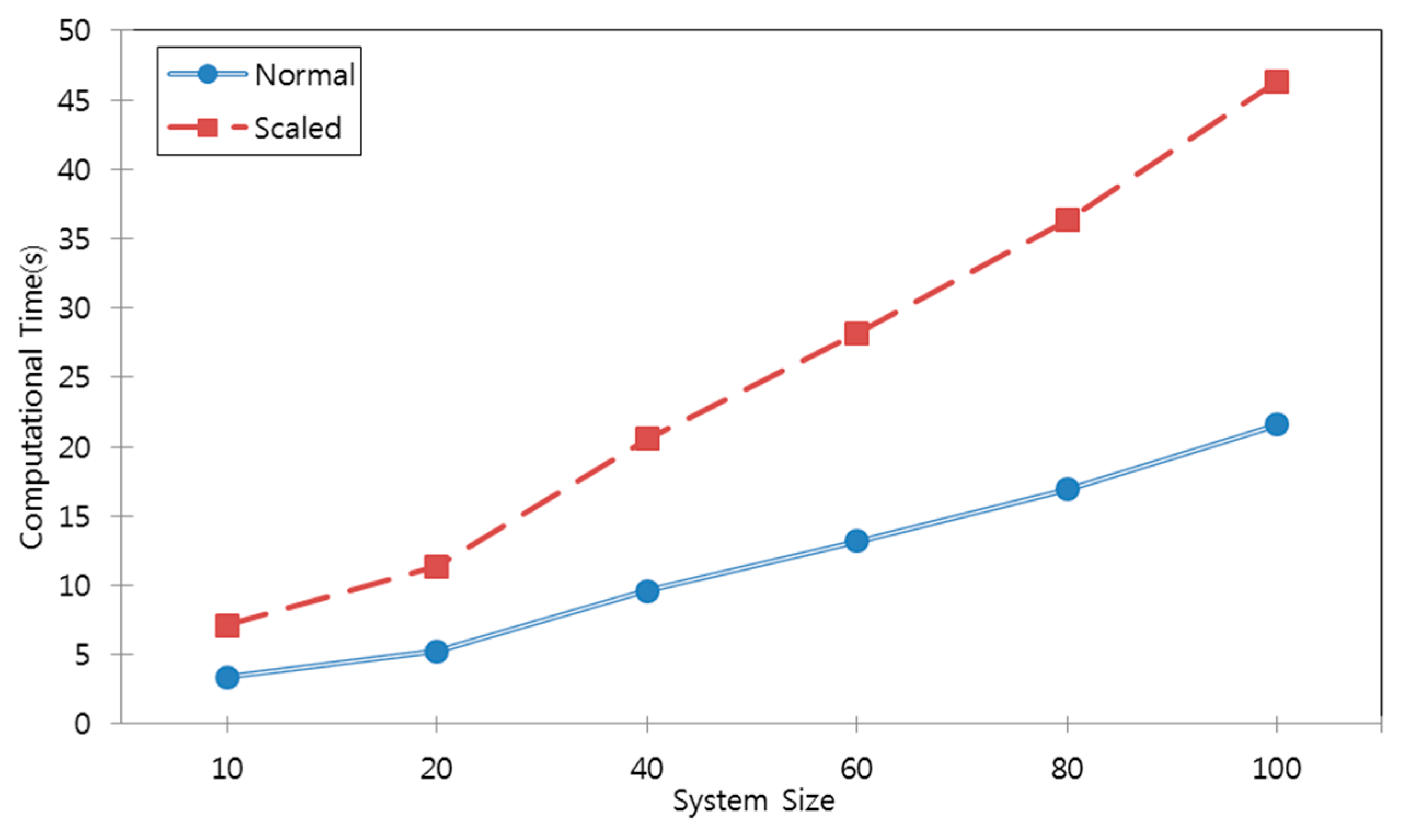
The computational time is a critical factor in proving the efficiency of the algorithm. However, because the computational time of an optimization algorithm is measured on different performance computers, it is necessary to standardize the time over the computational time measurements. Here, to show the efficiency of the algorithm, time is converted to values over a common base CPU (central processing unit) frequency of 1.5 GHz [29]. The computational time of the IGA is the average value of the 30 runs. The scaled time is computed as:
Table 2 shows the analysis of the algorithms in terms of performance. QBPSO requires the longest scaled computational time on most of the test systems, except for the 10-unit test system, because it requires a long time to iteratively linearize the objective function. Figure 6 illustrates the computational time of the IGA for each system size. The IGA has a fast computational time, and it possesses the desirable characteristic of a computational time that grows linearly with the system size. Unit decommitment and the reserve repairing need more execution time as the system size grows, whereas the computational framework of the IGA is less affected. Since the beginning search area of the IGA is an adjacent area, and the UC scheduling is highly likely to produce possible near-optimal schedules, the search convergence is significantly expedited for each unit size.
5.2. Result of UC Problem
A modified 24-h UC test system was used to schedule the UC problem [37]. In this system, we run the computational experiments at different forecast levels to compare the performance of each case. The capacity of solar and wind energy are supposed to be 100 MW and 200 MW, respectively. Thus, the total capacity of renewable sources is 300 MW, which is 20% of the peak load.
Table 3 shows four stochastic and five deterministic cases of UC strategies. The spinning reserve requirement of all of the deterministic cases is set to 10% of the load demand in the day-ahead UC scheduling. On the other hand, stochastic cases examine each reserve strategies with a prediction for renewable sources. Additional reserve requirements are set to recompense for the uncertainties that may not be covered by the basic spinning reserve. The summation for forecasting values of solar and wind power are also applied for setting different reserve strategies in the four stochastic cases. For each simulation case, 100 scenarios have been generated for each uncertainty of energy sources, such as wind, solar, load, and generator outage uncertainties.
Table 4 lists the scheduled operating cost in the day-ahead UC decision for each test case. For deterministic cases, one scenario is simulated with renewable energy, and the result is a single value of operating cost. When comparing four deterministic cases, the highest operating cost corresponds to the no-forecast case of Det1, because the cost of renewable generation is regarded as zero in this case. Certainly, the larger proportion of renewable generation penetration will lead to a smaller generation cost, and vice versa. The penetration of renewable sources is moderate in Det2, so operating cost also stays at moderate levels. Det4 obtains the second-highest operating cost because it uses a conservative 20% quantile forecast of renewable sources, while Det5 has the lowest cost of all of the deterministic cases due to the positive forecast. Therefore, the order of operating costs from the lowest to the highest is Det5 < Det2 < Det3 < Det4 < Det1.
In the stochastic cases, 100 scenarios are considered for the UIM for load and renewable source, and the cost is an expected value. As shown in Table 4, the result of the overall operating cost with the UIM is lower than that without the UIM in all of the cases. On the other hand, the reserve requirement with the UIM is higher than that without the UIM. The UIM complements the uncertainties with each other, thus reducing the total operating cost and reserve requirements. The order of the SUC cost and reserve requirement is the same with or without UIM. Therefore, operating costs from the lowest to the highest are Stc1 < Stc3 < Stc4 < Stc2.
Comparing the results of the deterministic and stochastic cases, it can be seen that there is a large difference in the operating cost between each case in the deterministic strategy. On the contrary in the stochastic cases, there is a relatively small difference in the operating cost. Since the probability of each deterministic case implies that it is more likely to differ from the real value than the stochastic cases, in the end, the stochastic strategy provides a better solution when making decisions to solve UC problems.
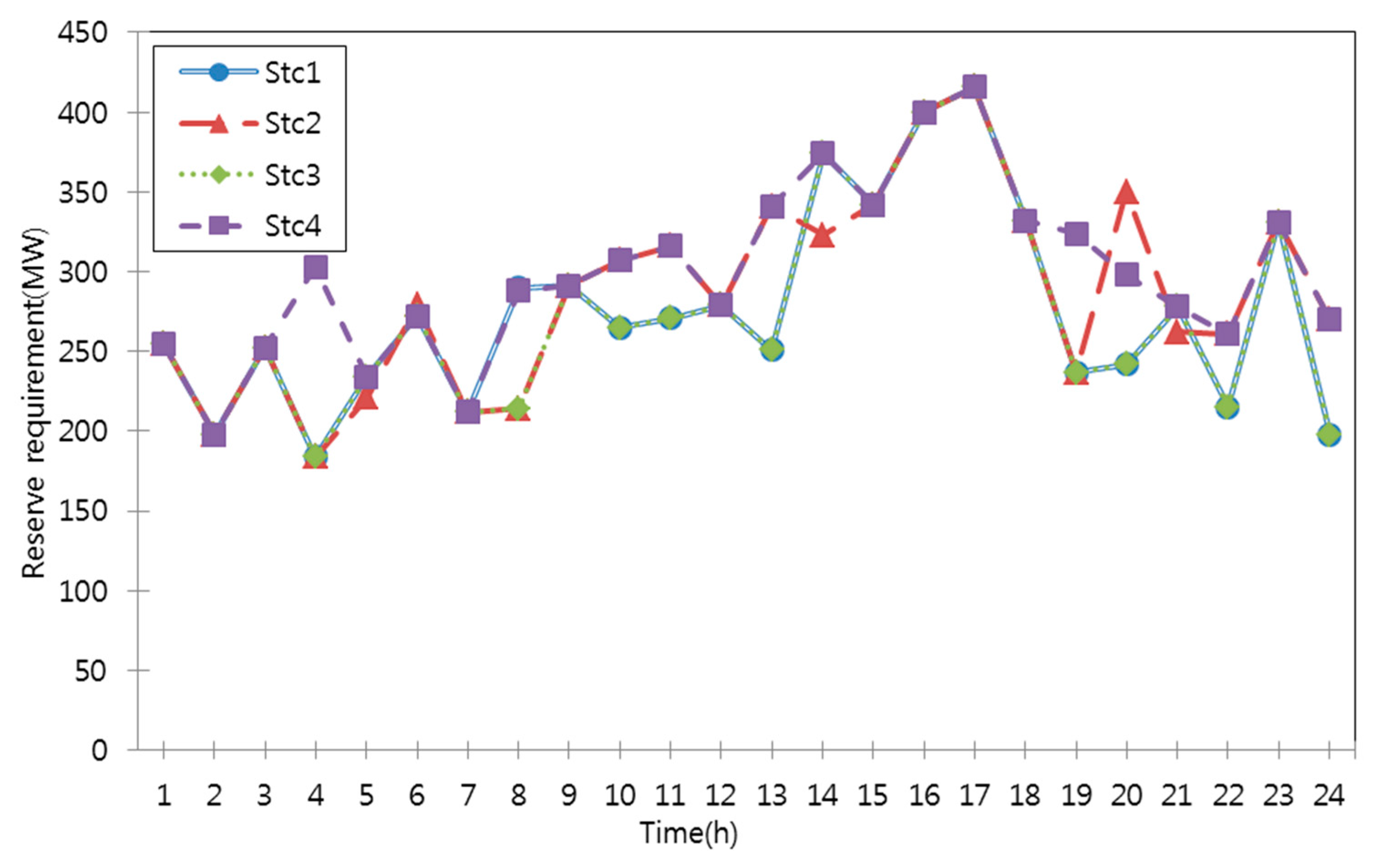
Figure 7 shows the results for the reserve requirement with the UIM. All of the UC strategies satisfied the reserve requirement for each hour. Depending on the uncertainty forecast, the total reserve requirement for each stochastic case may vary. It should be noted that according to the results of SUC scheduling and forecast, the reserve requirement to be secured varies during each hour. Stc1 is the standard case, and its level of the spinning reserve requirement and operating cost are the lowest of all the stochastic cases, whereas Stc2 required the highest reserve level and led to the highest cost.
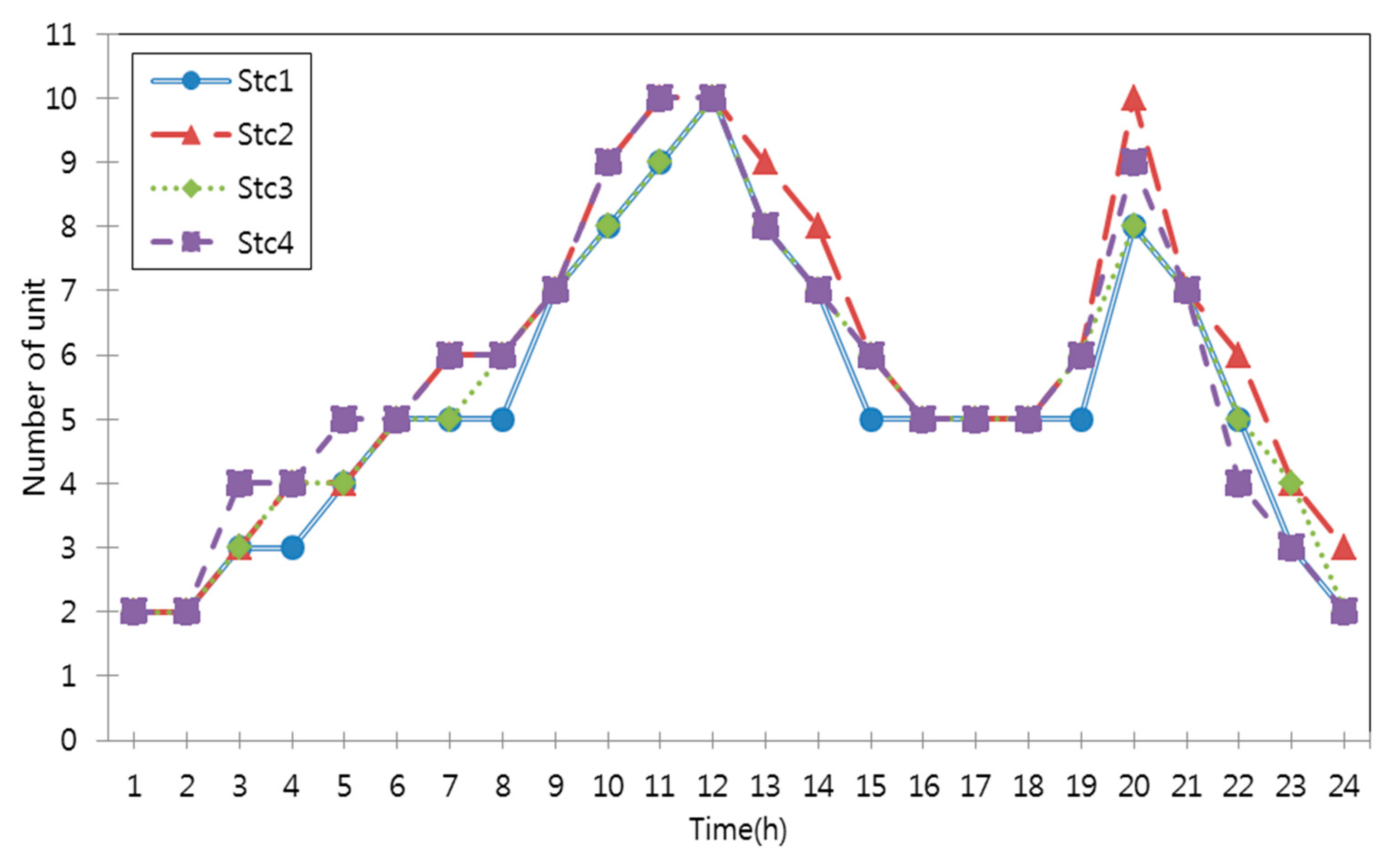
Figure 8 shows the number of turned-on units with the UIM. The on and off operation of each unit is closely related to the amount of reserve requirement. Stc1 has the fewest units turned on for most hour intervals. This is because Stc1 has a lesser reserve requirement than other cases. Conversely, Stc2 has the most units turned on for most hour intervals, because Stc2 has a higher reserve requirement (15% of load forecast) than the other stochastic cases. Additionally, the unit behavior of the best SUC solution for each case is shown in Appendix A.
6. Conclusions
In this paper, an IGA-based UC solution was proposed with the UIM considering renewable energy. Uncertainties of energy sources were supposed to have a normal distribution in a Monte Carlo simulation. To deal with uncertainties of various sources in the UC problem, the UIM was proposed by using a combination of scenarios that were selected considering the correlation of energy sources. The SUC problem was formulated with a simplified objective function by using the net load concept. To acquire better optimization results for the SUC problem, the IGA was applied, including an approximation process. To demonstrate the effectiveness of the IGA, computational time and operating costs were compared with other optimization methods for deterministic cases. The IGA showed better performance compared with other optimization methods. The UIM is the process of finding the best combination, considering the correlation of uncertainties based on the generated scenarios of load, wind, and solar power. It can also be seen that renewable energy source penetration can help relieve strict reserve requirements. Therefore, the system operator can obtain a suitable solution to determine unit scheduling with fast computational time through the proposed IGA-based SUC procedure. Further research work will focus on how to formulate more efficient SUC problems, including various operational constraints such as emission, transmission, and other services.
Author Contributions
Kyu-Hyung Jo proposed the main idea of this paper and Mun-Kyeom Kim coordinated the proposed approach in the manuscript.
Acknowledgments
This research was supported by the Basic Science Research Program through the National Research Foundation of Korea (NRF) funded by the Ministry of Education (2017R1D1A1B03029308).
Conflicts of Interest
The authors declare no conflict of interest.
Nomenclature
Constants
| πs | probability of scenario occurrence |
| FCg | fuel cost function of unit |
| Sg | unit’s start-up/shut down cost |
| ai, bi, ci | fuel cost coefficients of fitted parameters for each unit |
| SUg | unit’s start-up cost |
| SDg | unit’s shut-down cost |
| generator capacity value at minimum and maximum | |
| generator ramping rate value of maximum | |
| UTi, DTi | minimum up and down times for unit |
| RUg | unit’s ramping-up rate |
| SURg | unit’s start-up ramping rate |
| RDg | unit’s ramping-down rate |
| SDRg | unit’s shut-down ramping rate |
| Vc | cut-in speed of wind |
| Vo | cut-out speed of wind |
| Vr | rated speed of wind |
Variables
| Lst | load scenario at time t |
| Lforecasted,st | predicted value of load |
| Wgst | wind power of unit g |
| Wforecasted,st | predicted value of wind power |
| Sgst | solar power of unit g |
| Sforecasted,st | predicted value of solar power |
| WLRst | additional reserve requirement |
| Lerror,st | forecasting error of load |
| Werror,st | forecasting error of wind |
| Serror,st | forecasting error of solar |
| Rst | basic reserve requirement |
| Rgst | basic reserve requirement of unit g |
| maximum capacity of unit g | |
| pgst | power output of unit g |
| ugst | commitment of unit g |
| sgst | start-up binary indicator of unit g |
| xgst | shut-down binary indicator of generator g |
| minimum and maximum value of basic reserve requirement | |
| rated output of wind power | |
| USgst | up-spinning reserve of unit g |
| SUgst | start-up cost for unit g |
| ESTC | irradiance in standard condition |
| PSTC | maximum power in standard condition |
| k | temperature coefficient of the solar power |
| TM | temperature of solar module |
| TSTC | reference temperature |
Indices
| g | generator index |
| n | number of modules in the solar plant |
| s | scenario index |
| t | time index (hour) |
| st | scenario s at time t |
| gst | unit g at time t in scenario s |
| i | thermal unit index |
Appendix A

Table A1.
Unit State Combination of Stc1.
| Unit | Time (h) | |||||||||||||||||||||||
|---|---|---|---|---|---|---|---|---|---|---|---|---|---|---|---|---|---|---|---|---|---|---|---|---|
| 1 | 2 | 3 | 4 | 5 | 6 | 7 | 8 | 9 | 10 | 11 | 12 | 13 | 14 | 15 | 16 | 17 | 18 | 19 | 20 | 21 | 22 | 23 | 24 | |
| 1 | 1 | 1 | 1 | 1 | 1 | 1 | 1 | 1 | 1 | 1 | 1 | 1 | 1 | 1 | 1 | 1 | 1 | 1 | 1 | 1 | 1 | 1 | 1 | 1 |
| 2 | 1 | 1 | 1 | 1 | 1 | 1 | 1 | 1 | 1 | 1 | 1 | 1 | 1 | 1 | 1 | 1 | 1 | 1 | 1 | 1 | 1 | 1 | 1 | 1 |
| 3 | 0 | 0 | 0 | 0 | 1 | 1 | 1 | 1 | 1 | 1 | 1 | 1 | 1 | 1 | 0 | 0 | 0 | 0 | 0 | 1 | 1 | 1 | 1 | 0 |
| 4 | 0 | 0 | 0 | 0 | 0 | 1 | 1 | 1 | 1 | 1 | 1 | 1 | 1 | 1 | 1 | 1 | 1 | 1 | 1 | 1 | 1 | 1 | 0 | 0 |
| 5 | 0 | 0 | 0 | 1 | 1 | 1 | 1 | 1 | 1 | 1 | 1 | 1 | 1 | 1 | 1 | 1 | 1 | 1 | 1 | 1 | 1 | 1 | 0 | 0 |
| 6 | 0 | 0 | 0 | 0 | 0 | 0 | 0 | 0 | 1 | 1 | 1 | 1 | 1 | 1 | 1 | 1 | 1 | 1 | 1 | 1 | 1 | 0 | 0 | 0 |
| 7 | 0 | 0 | 0 | 0 | 0 | 0 | 0 | 0 | 1 | 1 | 1 | 1 | 1 | 1 | 0 | 0 | 0 | 0 | 0 | 1 | 1 | 0 | 0 | 0 |
| 8 | 0 | 0 | 1 | 0 | 0 | 0 | 0 | 0 | 0 | 1 | 1 | 1 | 1 | 0 | 0 | 0 | 0 | 0 | 0 | 0 | 0 | 0 | 0 | 0 |
| 9 | 0 | 0 | 0 | 0 | 0 | 0 | 0 | 0 | 0 | 0 | 1 | 1 | 0 | 0 | 0 | 0 | 0 | 0 | 0 | 0 | 0 | 0 | 0 | 0 |
| 10 | 0 | 0 | 0 | 0 | 0 | 0 | 0 | 0 | 0 | 0 | 0 | 1 | 0 | 0 | 0 | 0 | 0 | 0 | 0 | 1 | 0 | 0 | 0 | 0 |
Table A2.
Unit State Combination of Stc2.
| Unit | Time (h) | |||||||||||||||||||||||
|---|---|---|---|---|---|---|---|---|---|---|---|---|---|---|---|---|---|---|---|---|---|---|---|---|
| 1 | 2 | 3 | 4 | 5 | 6 | 7 | 8 | 9 | 10 | 11 | 12 | 13 | 14 | 15 | 16 | 17 | 18 | 19 | 20 | 21 | 22 | 23 | 24 | |
| 1 | 1 | 1 | 1 | 1 | 1 | 1 | 1 | 1 | 1 | 1 | 1 | 1 | 1 | 1 | 1 | 1 | 1 | 1 | 1 | 1 | 1 | 1 | 1 | 1 |
| 2 | 1 | 1 | 1 | 1 | 1 | 1 | 1 | 1 | 1 | 1 | 1 | 1 | 1 | 1 | 1 | 1 | 1 | 1 | 1 | 1 | 1 | 1 | 1 | 1 |
| 3 | 0 | 1 | 0 | 0 | 1 | 1 | 1 | 1 | 1 | 1 | 1 | 1 | 1 | 1 | 0 | 0 | 0 | 0 | 0 | 1 | 1 | 1 | 1 | 1 |
| 4 | 0 | 0 | 0 | 0 | 0 | 1 | 1 | 1 | 1 | 1 | 1 | 1 | 1 | 1 | 1 | 1 | 1 | 1 | 1 | 1 | 1 | 1 | 0 | 0 |
| 5 | 0 | 0 | 0 | 1 | 1 | 1 | 1 | 1 | 1 | 1 | 1 | 1 | 1 | 1 | 1 | 1 | 1 | 1 | 1 | 1 | 1 | 1 | 0 | 0 |
| 6 | 0 | 0 | 0 | 0 | 0 | 0 | 0 | 0 | 1 | 1 | 1 | 1 | 1 | 1 | 1 | 1 | 1 | 1 | 1 | 1 | 1 | 0 | 0 | 0 |
| 7 | 0 | 0 | 0 | 0 | 0 | 0 | 0 | 0 | 1 | 1 | 1 | 1 | 1 | 0 | 0 | 0 | 0 | 0 | 0 | 0 | 0 | 0 | 0 | 0 |
| 8 | 0 | 0 | 1 | 0 | 0 | 0 | 0 | 0 | 0 | 1 | 1 | 1 | 1 | 0 | 0 | 0 | 0 | 0 | 0 | 0 | 0 | 0 | 0 | 0 |
| 9 | 0 | 0 | 0 | 0 | 0 | 0 | 0 | 0 | 0 | 0 | 1 | 1 | 1 | 0 | 0 | 0 | 0 | 0 | 0 | 0 | 0 | 0 | 0 | 0 |
| 10 | 0 | 0 | 0 | 0 | 0 | 0 | 0 | 0 | 0 | 0 | 0 | 1 | 0 | 0 | 0 | 0 | 0 | 0 | 0 | 1 | 0 | 0 | 0 | 0 |
Table A3.
Unit State Combination of Stc3.
| Unit | Time (h) | |||||||||||||||||||||||
|---|---|---|---|---|---|---|---|---|---|---|---|---|---|---|---|---|---|---|---|---|---|---|---|---|
| 1 | 2 | 3 | 4 | 5 | 6 | 7 | 8 | 9 | 10 | 11 | 12 | 13 | 14 | 15 | 16 | 17 | 18 | 19 | 20 | 21 | 22 | 23 | 24 | |
| 1 | 1 | 1 | 1 | 1 | 1 | 1 | 1 | 1 | 1 | 1 | 1 | 1 | 1 | 1 | 1 | 1 | 1 | 1 | 1 | 1 | 1 | 1 | 1 | 1 |
| 2 | 1 | 1 | 1 | 1 | 1 | 1 | 1 | 1 | 1 | 1 | 1 | 1 | 1 | 1 | 1 | 1 | 1 | 1 | 1 | 1 | 1 | 1 | 1 | 1 |
| 3 | 0 | 0 | 0 | 0 | 1 | 1 | 1 | 1 | 1 | 1 | 1 | 1 | 1 | 1 | 0 | 0 | 0 | 0 | 0 | 1 | 1 | 1 | 1 | 1 |
| 4 | 0 | 0 | 0 | 0 | 0 | 1 | 1 | 1 | 1 | 1 | 1 | 1 | 1 | 1 | 1 | 1 | 1 | 1 | 1 | 1 | 1 | 1 | 0 | 0 |
| 5 | 0 | 0 | 0 | 1 | 1 | 1 | 1 | 1 | 1 | 1 | 1 | 1 | 1 | 1 | 1 | 1 | 1 | 1 | 1 | 1 | 1 | 0 | 0 | 0 |
| 6 | 0 | 0 | 0 | 0 | 0 | 0 | 0 | 0 | 1 | 1 | 1 | 1 | 1 | 1 | 1 | 1 | 1 | 1 | 1 | 1 | 1 | 0 | 0 | 0 |
| 7 | 0 | 0 | 0 | 0 | 0 | 0 | 0 | 0 | 1 | 1 | 1 | 1 | 1 | 1 | 0 | 0 | 0 | 0 | 0 | 1 | 0 | 0 | 0 | 0 |
| 8 | 0 | 0 | 1 | 0 | 0 | 0 | 0 | 0 | 0 | 1 | 1 | 1 | 1 | 0 | 0 | 0 | 0 | 0 | 0 | 0 | 0 | 0 | 0 | 0 |
| 9 | 0 | 0 | 0 | 0 | 0 | 0 | 0 | 0 | 0 | 0 | 1 | 1 | 0 | 0 | 0 | 0 | 0 | 0 | 0 | 0 | 0 | 0 | 0 | 0 |
| 10 | 0 | 0 | 0 | 0 | 0 | 0 | 0 | 0 | 0 | 0 | 1 | 0 | 0 | 0 | 0 | 0 | 0 | 0 | 0 | 0 | 0 | 0 | 0 | 0 |
Table A4.
Unit State Combination of Stc4.
| Unit | Time (h) | |||||||||||||||||||||||
|---|---|---|---|---|---|---|---|---|---|---|---|---|---|---|---|---|---|---|---|---|---|---|---|---|
| 1 | 2 | 3 | 4 | 5 | 6 | 7 | 8 | 9 | 10 | 11 | 12 | 13 | 14 | 15 | 16 | 17 | 18 | 19 | 20 | 21 | 22 | 23 | 24 | |
| 1 | 1 | 1 | 1 | 1 | 1 | 1 | 1 | 1 | 1 | 1 | 1 | 1 | 1 | 1 | 1 | 1 | 1 | 1 | 1 | 1 | 1 | 1 | 1 | 1 |
| 2 | 1 | 1 | 1 | 1 | 1 | 1 | 1 | 1 | 1 | 1 | 1 | 1 | 1 | 1 | 1 | 1 | 1 | 1 | 1 | 1 | 1 | 1 | 1 | 1 |
| 3 | 0 | 0 | 0 | 0 | 1 | 1 | 1 | 1 | 1 | 1 | 1 | 1 | 1 | 1 | 0 | 0 | 0 | 0 | 0 | 1 | 1 | 1 | 1 | 0 |
| 4 | 0 | 0 | 0 | 0 | 0 | 1 | 1 | 1 | 1 | 1 | 1 | 1 | 1 | 1 | 1 | 1 | 1 | 1 | 1 | 1 | 1 | 1 | 0 | 0 |
| 5 | 0 | 0 | 0 | 1 | 1 | 1 | 1 | 1 | 1 | 1 | 1 | 1 | 1 | 1 | 1 | 1 | 1 | 1 | 1 | 1 | 1 | 1 | 0 | 0 |
| 6 | 0 | 0 | 0 | 0 | 0 | 0 | 0 | 0 | 1 | 1 | 1 | 1 | 1 | 1 | 1 | 1 | 1 | 1 | 1 | 1 | 1 | 0 | 0 | 0 |
| 7 | 0 | 0 | 0 | 0 | 0 | 0 | 0 | 0 | 1 | 1 | 1 | 1 | 1 | 1 | 0 | 0 | 0 | 0 | 0 | 1 | 1 | 0 | 0 | 0 |
| 8 | 0 | 0 | 1 | 0 | 0 | 0 | 0 | 0 | 0 | 1 | 1 | 1 | 1 | 1 | 0 | 0 | 0 | 0 | 0 | 0 | 0 | 0 | 0 | 0 |
| 9 | 0 | 0 | 0 | 0 | 0 | 0 | 0 | 0 | 0 | 0 | 1 | 1 | 1 | 0 | 0 | 0 | 0 | 0 | 0 | 0 | 0 | 0 | 0 | 0 |
| 10 | 0 | 0 | 0 | 0 | 0 | 0 | 0 | 0 | 0 | 0 | 0 | 0 | 1 | 0 | 0 | 0 | 0 | 0 | 0 | 1 | 0 | 0 | 0 | 0 |
References
- Min, C.G.; Kim, M.K. Net Load Carrying Capability of Generating Units in Power Systems. Energies 2017, 10, 1221. [Google Scholar] [CrossRef]
- Ji, B.; Yuan, X.; Chen, Z.; Tian, H. Improved gravitational search algorithm for unit commitment considering uncertainty of wind power. Energy 2014, 67, 52–62. [Google Scholar] [CrossRef]
- Ko, W.; Park, J.-K.; Kim, M.-K.; Heo, J.-H. A Multi-Energy System Expansion Planning Method Using a Linearized Load-Energy Curve A Case Study in South Korea. Energies 2017, 10, 1663. [Google Scholar] [CrossRef]
- Cheng, Y.; Lai, C. Control Strategy Optimization for Parallel Hybrid Electric Vehicles Using a Memetic Algorithm. Energies 2017, 10, 305. [Google Scholar] [CrossRef]
- Kishore, C.; Ghosh, S.; Karar, V. Symmetric Fuzzy Logic and IBFOA Solutions for Optimal Position and Rating of Capacitors Allocated to Radial Distribution Networks. Energies 2018, 11, 766. [Google Scholar] [CrossRef]
- Bai, Y.; Zhong, H.; Xia, Q.; Kang, C.; Xie, L. A decomposition method for network-constrained unit commitment with AC power flow constraints. Energy 2015, 88, 595–603. [Google Scholar] [CrossRef]
- Hengrui, M.; Bo, W.; Wenzhong, G.; Dichen, L.; Yong, S.; Zhijun, L. Optimal Scheduling of an Regional Integrated Energy System with Energy Storage Systems for Service Regulation. Energies 2018, 11, 195. [Google Scholar] [CrossRef]
- Jianzhong, Z.; Yanhe, X.; Yang, Z.; Yuncheng, Z. Optimization of Guide Vane Closing Schemes of Pumped Storage Hydro Unit Using an Enhanced Multi-Objective Gravitational Search Algorithm. Energies 2015, 109, 765–780. [Google Scholar]
- Mohamed, A.T.; Hegazy, R.; Vladimir, T.; Ahmed, A.Z.D.; Almoataz, Y.A.; Artem, V. Impact of Optimum Allocation of Renewable Distributed Generations on Distribution Networks Based on Different Optimization Algorithms. Energies 2018, 11, 245. [Google Scholar] [CrossRef]
- Luis, A.C.R.; Dalila, B.M.M.F.; Fernando, A.C.C.F. A Metaheuristic Approach to the Multi-Objective Unit Commitment Problem Combining Economic and Environmental Criteria. Energies 2017, 10, 2029. [Google Scholar] [CrossRef]
- Liang, R.-H.; Liao, J.-H. A fuzzy-optimization approach for generation scheduling with wind and solar energy systems. IEEE Trans. Power Syst. 2007, 22, 1665–1674. [Google Scholar] [CrossRef]
- Niknam, T.; Azizipanah-Abarghooee, R.; Narimani, M.R. An efficient scenariobased stochastic programming framework for multi-objective optimal microgrid operation. Appl. Energy 2012, 99, 455–470. [Google Scholar] [CrossRef]
- Wu, L.; Shahidehpour, M.; Li, Z. Comparison of scenario-based and interval optimization approaches to stochastic SCUC. IEEE Trans. Power Syst. 2012, 27, 913–921. [Google Scholar] [CrossRef]
- Kuznetsova, E.; Li, Y.-F.; Ruiz, C.; Zio, E. An integrated framework of agent-based modelling and robust optimization for microgrid energy management. Appl. Energy 2014, 129, 70–88. [Google Scholar] [CrossRef]
- Zhang, Y.; Wang, J.; Ding, T.; Wang, X. Conditional value at risk-based stochastic unit commitment considering the uncertainty of wind power generation. IET Gener. Transm. Distrib. 2018, 12, 482–489. [Google Scholar] [CrossRef]
- Jiang, R.; Wang, J.; Guan, Y. Robust unit commitment with wind power and pumped storage hydro. IEEE Trans. Power Syst. 2012, 27, 800–810. [Google Scholar] [CrossRef]
- Bertsimas, D.; Litvinov, E.; Sun, X.; Zhao, J.; Zheng, T. Adaptive robust optimization for the security constrained unit commitment problem. IEEE Trans. Power Syst. 2013, 28, 52–63. [Google Scholar] [CrossRef]
- Anand, H.; Narang, N.; Dhillon, J.S. Profit based unit commitment using hybrid optimization technique. Energy 2018, 148, 701–715. [Google Scholar] [CrossRef]
- Fattahi, S.; Ashraphijuo, M.; Lavaei, J.; Atamturk, A. Conic relaxations of the unit commitment problem. Energy 2017, 134, 1079–1095. [Google Scholar] [CrossRef]
- Moshoko, E.; Caston, S.; Alphonce, B.; Robert, F.; John, E.B. Short term electricity demand forecasting using partially linear additive quantile regression with an application to the unit commitment problem. Appl. Energy 2018, 222, 104–118. [Google Scholar]
- Reddy, G.V.S.; Ganesh, V.; Rao, C.S. Implementation of clustering based unit commitment employing imperialistic competition algorithm. Int. J. Elec. Power Energy Syst. 2016, 82, 621–628. [Google Scholar]
- Wang, Q.; Guan, Y.; Wang, J. A Chance-Constrained Two-Stage Stochastic Program for Unit Commitment with Uncertain Wind Power Output. IEEE Trans. Power Syst. 2012, 27, 206–215. [Google Scholar] [CrossRef]
- Heo, S.Y.; Kim, M.K.; Choi, J.W. Hybrid Intelligent Control Method to Improve the Frequency Support Capability of Wind Energy Conversion Systems. Energies 2015, 8, 11430–11451. [Google Scholar] [CrossRef]
- Matos, M.A.; Bessa, R.J. Setting the operating reserve using probabilistic wind power forecasts. IEEE Trans. Power Syst. 2011, 26, 594–603. [Google Scholar] [CrossRef]
- Bo, W.; Shuming, W.; Xianzhong, Z.; Junzo, W. Multi-objective unit commitment with wind penetration and emission concerns under stochastic and fuzzy uncertainties. Energy 2016, 111, 18–31. [Google Scholar]
- Emmanouil, A.; Christos, K.; Pandelis, N.; Anastasios, G. Storage management by rolling stochastic unit commitment for high renewable energy penetration. Electr. Power Syst. Res. 2018, 158, 240–249. [Google Scholar]
- Mohsen, N.; Martin, B.; Stefan, T. Optimization of unit commitment and economic dispatch in microgrids based on genetic algorithm and mixed integer linear programming. Appl. Energy 2018, 210, 944–963. [Google Scholar]
- Chen, P.H. Two-level hierarchical approach to unit commitment using expert system and elite PSO. IEEE Trans. Power Syst. 2012, 27, 780–789. [Google Scholar] [CrossRef]
- Yu, X.; Zhang, X. Unit commitment using Lagrangian relaxation and particle swarm optimization. Electr. Power Energy Syst. 2014, 61, 510–522. [Google Scholar] [CrossRef]
- Benhamida, F.; Abdelbar, B. Enhanced Lagrangian relaxation solution to the generation scheduling problem. Int. J. Electr. Power Energy Syst. 2010, 32, 1099–1105. [Google Scholar] [CrossRef]
- Juste, K.A.; Kita, H.; Tanaka, E.; Hasegawa, J. An evolutionary programming solution to the unit commitment problem. IEEE Trans. Power Syst. 1999, 14, 1452–1459. [Google Scholar] [CrossRef]
- Kazarlis, S.A.; Bakirtzis, A.G.; Petridis, V. A genetic algorithm solution to the unit commitment problem. IEEE Trans. Power Syst. 1996, 11, 83–92. [Google Scholar] [CrossRef]
- Balci, H.H.; Valenzuela, J.F. Scheduling electric power generators using particle swarm optimization combined with the Lagrangian relaxation method. Int. J. Appl. Math. Comput. Sci. 2004, 14, 411–421. [Google Scholar]
- Yuan, X.H.; Nie, H.; Su, A.J.; Wang, L.; Yuan, Y.B. An improved binary particle swarm optimization for unit commitment problem. Expert Syst. Appl. 2009, 36, 8049–8055. [Google Scholar] [CrossRef]
- Jeong, Y.W.; Park, J.B.; Jang, S.H.; Lee, K.Y. A new quantum-inspired binary PSO: Application to unit commitment problems for power systems. IEEE Trans. Power Syst. 2010, 25, 1486–1495. [Google Scholar] [CrossRef]
- Lee, K.Y.; Cha, Y.T.; Park, J.H. Short-term load forecasting using an artificial neural network. IEEE Trans. Power Syst. 1992, 7, 124–132. [Google Scholar] [CrossRef]
- Ongsakul, W.; Petcharaks, N. Unit commitment by enhanced adaptive Lagrangian relaxation. IEEE Trans. Power Syst. 2004, 19, 620–628. [Google Scholar] [CrossRef]
Figure 1.
Probability Distribution of the Uncertainty Forecasting.

Figure 2.
Structure of the uncertainty integration method (UIM).

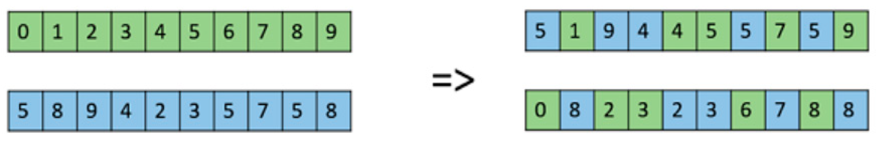
Figure 3.
Crossover operator.

Figure 4.
Swap mutation operator.

Figure 5.
Solution process of improved genetic algorithm (IGA)-based stochastic unit commitment (SUC) problem.
Figure 5.
Solution process of improved genetic algorithm (IGA)-based stochastic unit commitment (SUC) problem.

Figure 6.
IGA computational time for each system size.

Figure 7.
Reserve requirement with the UIM.

Figure 8.
Number of units turned on with the UIM.

Table 1.
Comparison of operating costs.
| Algorithms | Generation Cost ($) for Each Unit Size | ||||||
|---|---|---|---|---|---|---|---|
| 10 | 20 | 40 | 60 | 80 | 100 | ||
| PSO [32] | Best | 563,977 | 1,124,038 | 2,243,256 | 3,362,881 | 4,482,940 | 5,603,749 |
| Average | 564,502 | 1,125,406 | 2,245,966 | 3,366,801 | 4,488,982 | 5,609,274 | |
| Worst | 565,186 | 1,125,836 | 2,247,688 | 3,368,559 | 4,493,069 | 5,611,131 | |
| LR [30] EP [28] GA [29] | 563,938 | 1,122,637 | 2,243,245 | 3,363,376 | 4,484,915 | 5,604,470 | |
| Best | 564,551 | 1,125,494 | 2,249,093 | 3,371,611 | 4,498,479 | 5,623,885 | |
| Best | 565,825 | 1,126,243 | 2,251,911 | 3,376,625 | 4,504,933 | 5,627,437 | |
| ES-PSO [31] | Best | 563,938 | 1,123,003 | 2,242,167 | 3,362,084 | 4,481,863 | 5,602,039 |
| Average | 563,942 | 1,123,474 | 2,243,517 | 3,364,719 | 4,483,992 | 5,603,815 | |
| Worst | 563,977 | 1,124,540 | 2,246,305 | 3,368,112 | 4,487,569 | 5,606,491 | |
| PSO-LR [33] | Best | 565,869 | 1,128,072 | 2,251,116 | 3,376,407 | 4,496,717 | 5,623,607 |
| IBPSO [34] | Best | 563,977 | 1,125,216 | 2,248,581 | 3,367,865 | 4,491,083 | 5,610,293 |
| Average | 564,155 | 1,125,448 | 2,248,875 | 3,368,278 | 4,491,681 | 5,611,181 | |
| Worst | 565,312 | 1,125,730 | 2,249,302 | 3,368,779 | 4,492,686 | 5,612,265 | |
| QBPSO [35] | Best | 563,977 | 1,123,297 | 2,242,957 | 3,361,980 | 4,482,085 | 5,602,486 |
| Average | 563,977 | 1,123,981 | 2,244,657 | 3,363,763 | 4,485,410 | 5,604,275 | |
| Worst | 563,977 | 1,124,294 | 2,245,941 | 3,365,707 | 4,487,168 | 5,606,178 | |
| IGA | Best | 564,037 | 1,122,035 | 2,242,031 | 3,360,324 | 4,481,714 | 5,601,771 |
| Average | 564,314 | 1,122,216 | 2,242,217 | 3,360,514 | 4,481,896 | 5,601,924 | |
| Worst | 564,537 | 1,122,424 | 2,242,462 | 3,360,717 | 4,482,028 | 5,602,136 | |
Table 2.
Comparison of computational time.
| Algorithms | Normal/Scaled | Computational Time (s) for Each Unit Size | |||||
|---|---|---|---|---|---|---|---|
| 10 | 20 | 40 | 60 | 80 | 100 | ||
| LR [30] | Normal | 10 | 14 | 25 | 39 | 64 | 80 |
| Scaled | 11.5 | 16.2 | 28.8 | 44.9 | 73.8 | 92.2 | |
| EP [28] | Normal | 100 | 340 | 1176 | 2267 | 3584 | 6120 |
| Scaled | 10.6 | 36.2 | 125.4 | 241.8 | 382.2 | 652.8 | |
| GA [29] | Normal | 221 | 733 | 2697 | 5840 | 10,036 | 15,733 |
| Scaled | 7.3 | 24.4 | 89.9 | 194.6 | 334.5 | 524.4 | |
| ES-PSO [31] | Normal | 12 | 19 | 42 | 56 | 113 | 162 |
| Scaled | 19.2 | 30.4 | 67.2 | 89.6 | 180.8 | 259.2 | |
| PSO-LR [33] | Normal | 42 | 91 | 213 | 360 | 543 | 730 |
| Scaled | 28 | 60.6 | 142 | 240 | 362 | 486.6 | |
| IBPSO [34] | Normal | 27 | 55 | 110 | 172 | 235 | 295 |
| Scaled | 27 | 55 | 110 | 172 | 235 | 295 | |
| QBPSO [35] | Normal | 18 | 50 | 158 | 328 | 554 | 833 |
| Scaled | 24 | 66.67 | 210.6 | 437.3 | 738.6 | 1110.6 | |
| IGA | Normal | 3.4 | 5.25 | 9.6 | 13.2 | 16.9 | 21.6 |
| Scaled | 7.1 | 11.4 | 20.5 | 28.2 | 36.3 | 46.3 | |
Table 3.
Unit commitment (UC) strategies.
| Case | Descriptions | UC |
|---|---|---|
| Det1 | No forecast | Deterministic |
| Det2 | Point forecast | |
| Det3 | Perfect forecast | |
| Det4 | 20% quantile forecast | |
| Det5 | 80% quantile forecast | |
| Stc1 | Standard reserve (Load forecast (10%)) | Stochastic |
| Stc2 | Additional reserve (Load forecast (15%)) | |
| Stc3 | Additional reserve (Point forecast (50%)) | |
| Stc4 | Additional reserve (Point forecast − quantile forecast (10%)) |
Table 4.
Comparison of UC operating costs and reserve requirement.
| Approach | Case | Operating Cost ($) | Reserve Requirement (MW) | Value | |
|---|---|---|---|---|---|
| Deterministic | Det1 | 564,037.89 | 4320 | Single | |
| Det2 | 520,075.37 | 6684 | Single | ||
| Det3 | 524,832.56 | 6791 | Single | ||
| Det4 | 539,245.17 | 7124 | Single | ||
| Det5 | 496,781.24 | 6418 | Single | ||
| Stochastic | Without UIM | Stc1 | 535,827.21 | 6935 | Forecast |
| Stc2 | 544,177.81 | 7273 | Forecast | ||
| Stc3 | 539,124.56 | 7162 | Forecast | ||
| Stc4 | 539,651.24 | 7184 | Forecast | ||
| With UIM | Stc1 | 521,024.26 | 6733 | Forecast | |
| Stc2 | 536,544.17 | 7076 | Forecast | ||
| Stc3 | 535,926.34 | 6943 | Forecast | ||
| Stc4 | 536,274.94 | 6989 | Forecast | ||
© 2018 by the authors. Licensee MDPI, Basel, Switzerland. This article is an open access article distributed under the terms and conditions of the Creative Commons Attribution (CC BY) license (http://creativecommons.org/licenses/by/4.0/).
Share and Cite
MDPI and ACS Style
Jo, K.-H.; Kim, M.-K. Improved Genetic Algorithm-Based Unit Commitment Considering Uncertainty Integration Method. Energies 2018, 11, 1387. https://doi.org/10.3390/en11061387
AMA Style
Jo K-H, Kim M-K. Improved Genetic Algorithm-Based Unit Commitment Considering Uncertainty Integration Method. Energies. 2018; 11(6):1387. https://doi.org/10.3390/en11061387
Chicago/Turabian StyleJo, Kyu-Hyung, and Mun-Kyeom Kim. 2018. "Improved Genetic Algorithm-Based Unit Commitment Considering Uncertainty Integration Method" Energies 11, no. 6: 1387. https://doi.org/10.3390/en11061387
Note that from the first issue of 2016, this journal uses article numbers instead of page numbers. See further details here.