Geothermal-Related Thermo-Elastic Fracture Analysis by Numerical Manifold Method

Abstract

One significant factor influencing geothermal energy exploitation is the variation of the mechanical properties of rock in high temperature environments. Since rock is typically a heterogeneous granular material, thermal fracturing frequently occurs in the rock when the ambient temperature changes, which can greatly influence the geothermal energy exploitation. A numerical method based on the numerical manifold method (NMM) is developed in this study to simulate the thermo-elastic fracturing of rocklike granular materials. The Voronoi tessellation is incorporated into the pre-processor of NMM to represent the grain structure. A contact-based heat transfer model is developed to reflect heat interaction among grains. Based on the model, the transient thermal conduction algorithm for granular materials is established. To simulate the cohesion effects among grains and the fracturing process between grains, a damage-based contact fracture model is developed to improve the contact algorithm of NMM. In the developed numerical method, the heat interaction among grains as well as the heat transfer inside each solid grain are both simulated. Additionally, as damage evolution and fracturing at grain interfaces are also considered, the developed numerical method is applicable to simulate the geothermal-related thermal fracturing process.

1. Introduction

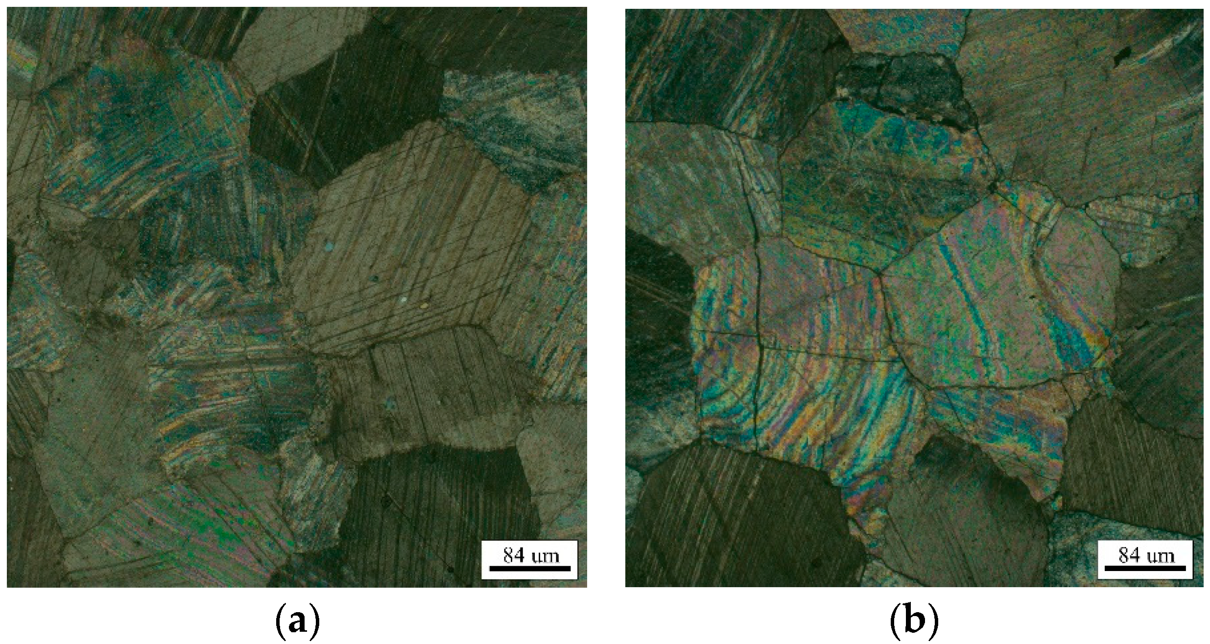
Geothermal energy is one of the most abundant renewable energies on the Earth. Its environmental friendliness and reliable features compared with the conventional fossil fuels greatly encourage further exploration and exploitation of geothermal energy. One significant factor that influences the exploitation of geothermal energy is the variation of the mechanical properties of rock in high temperature environments [1,2,3]. Therefore, investigating the thermo-mechanical mechanism of rock behavior under different thermal circumstances is attracting more and more attention nowadays. As a powerful and fundamental research approach, a great deal of laboratory tests have been conducted to investigate the thermo-mechanical mechanisms of rock. Based on laboratory tests, scholars have found that rocks are typical heterogeneous granular materials and the heterogeneity of rocks are mainly attributed to their random shaped mineral grains, cemented interfaces as well as microdefects (Figure 1a) [4,5,6]. The heterogeneity of rock can dramatically influence the thermal and mechanical properties of rocks. Under thermal circumstances, the random shaped grain structure of rock can bring about high temperature gradients, uncoordinated thermal stresses and strains [7]. Consequently, thermal fracturing of rocks occurs frequently (Figure 1b), which is an important factor that should be considered during geothermal energy exploitation. Thus, investigating the thermal fracturing process of rocklike granular material is of great importance for revealing the thermo-mechanical mechanism of the rock and improving the geothermal exploitation technologies. Indeed, considerable achievements have been attained based on laboratory tests. However, carrying out large numbers of laboratory tests is time-wasting and costly. Additionally, it is still difficult to completely monitor the micro failure process of materials in laboratory tests. Since rock are typical heterogeneous granular materials, developing numerical methods to investigate the thermal fracture effects of the rocklike granular materials is of great significance.

To date, numerous kinds of numerical simulations have been conducted to investigate the thermal fracture effects of different kinds of materials. Via incorporating fracture mechanics, many numerical simulations focus on evaluating the thermal stress intensity factors of originally existing fractures, which is essential for predicting the thermal induced fracture propagation. During these numerical investigations, the continuum-based numerical methods, i.e., the finite element method (FEM) [8], the extended finite element method (XFEM) [9], the meshless methods (MMs) [10] and the boundary element methods (BEMs) [11], are generally adopted. However, due to the limited capacities of the continuum-based numerical methods in simulating complex discontinuous geometries as well as the fracture mechanics on treating complex fracture patterns, only simple macroscale thermal fracture problems are studied in these numerical simulations.

Since the thermal fracturing of rocklike materials are greatly affected by their microstructure, continuum-based microscale thermo-mechanical coupling numerical algorithms are also developed to investigate the thermal fracturing process of granular materials. One typical example is the RFPA-thermal software developed by the Tang’s group [12], which is also an extension of the FEM. The RFPA-thermal represents the micro structure of rock with square finite elements. Through the incorporation of the statistically distributed material parameters and the thermo-elastic damage constitutive law, complex thermal fracturing from microscale to macroscale can be simulated by the RFPA-thermal method. However, since the displacements at the square grain boundaries are continuously simulated, the fracture paths are not explicitly represented in the RFPA-thermal.

Since the continuous numerical methods run into difficulties when simulating thermal fracturing of granular materials, the discontinuous numerical methods are also widely adopted to deal with such problems [13,14,15,16]. One widely used discontinuous numerical method for thermal fracturing is the particle flow code (PFC), in which the micrograins are represented by circular or spherical elements [13]. Incorporating the grain-based model and cluster model, which bond the same types of circular or spherical elements together, the PFC can realistically represent the grain structures of the rock [4]. Thus, complex thermal fracturing processes that consider the micro structure of rock are simulated [3,14,17]. As alternatives to the circle or sphere assembly-based numerical methods described above, polygon assembly-based simulations, such as the Voronoi polygon assembly-based simulations of Universal Distinct Element Code (UDEC) [18] and the triangular block assembly-based simulations of Discontinuous Deformation Analysis (DDA), are also extensively adopted in thermo-mechanical coupling problems [15]. By incorporating a contact-based fracture criterion, complex thermal fracturing of rock can also be successfully simulated by the polygon assembly-based numerical methods. In the above discontinuous particle assembly numerical methods, one temperature degree of freedom is assigned to each grain to simulate the heat transfer process. The heat transfer of the material are then approximated by the heat transfer among blocks and the heat transfer inside each polygonal grain is generally ignored [15,18]. Therefore, to obtain accurate temperature results, fine grain size, which means more temperature degrees of freedom, is generally necessary in these numerical methods. Additionally, the discontinuous numerical methods also run into difficulties in capturing the complex deformation field inside solid grains.

Since both the continuous and discontinuous numerical methods suffer limitations, combined continuous-discontinuous numerical methods have been developed during the past two decades. One of the most popular combined numerical methods is the numerical manifold method (NMM) [19]. The NMM inherits the contact theory of the DDA and adopts dual cover systems, i.e., the mathematical cover (MC) and the physical cover (PC), thus providing unique advantages for modelling continuous and discontinuous problems on a unified numerical platform. Therefore, the NMM has been widely applied to simulate both continuous and discontinuous problems [20,21,22,23,24,25,26,27,28,29,30,31,32,33,34,35,36,37]. Nowadays, the NMM has also been extended to model thermo-mechanical fracture problems by Zhang [38,39]. However, only thermal fracture stress intensity factors were investigated in Zhang’s study.

Considering the advantages of the NMM in simulating both continuous and discontinuous problems, the NMM is extended to analyze the thermal fracturing of the rocklike granular materials. Since laboratory experiments have revealed that the microstructure of rocklike granular materials appear more like random polygons [40], in this study random Voronoi polygon assemblies are constructed to approximate the microstructure of the granular materials. Basically, two separate heat transfer processes should be considered, i.e., the heat transfer in solid grains and the heat interactions among grains. To more realistically simulate the heat interactions among grains, a contact-based heat transfer model is developed based on the contact algorithm of NMM. Then the transient heat transfer algorithm is discretized and incorporated into the NMM platform. Additionally, a damage-based contact fracture model is developed to reflect the bonding-cracking mechanism of grain boundaries. Since both the heat transfer in the solid grain and the heat interactions among grains are considered, the developed numerical method can better simulate the heterogeneous heat transfer process of rocklike granular materials. Additionally, as damage evolution and fracturing at grain interfaces is also considered, the developed numerical method is applicable to simulate the geothermal-related thermal fracturing process. Two simple examples are simulated to validate the developed NMM algorithm. Then, the extended NMM algorithm is applied to investigate the thermal fracturing processes induced by elevated temperature and cooling respectively.

2. Methods and Backgrounds

2.1. Basic Concept of NMM

2.1.1. Cover System

The most distinctive feature of the NMM is its dual coverage system, i.e., the mathematical cover and the physical cover, which have already been elaborated in many references [22]. Attributed to the dual cover system, the NMM is capable of handling problems with complex physical meshes, such as cracks, holes, material interfaces, etc. The mathematical cover of NMM is a collection of small patches which can be of arbitrary shape and in theory it does not need to be consistent with the physical meshes. Thus, it is convenient to construct a numerical model with complex physical meshes in the NMM. Generally, the mathematical cover patches may partly overlap with each other and should cover the whole problem domain. In addition, the mathematical cover might intersect with the physical meshes. The subdivisions of the mathematical cover by the physical meshes are termed as the physical cover in NMM. The intersection of different physical covers is the manifold elements (ME) of NMM.

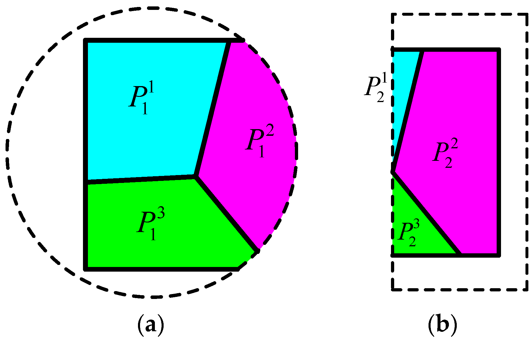
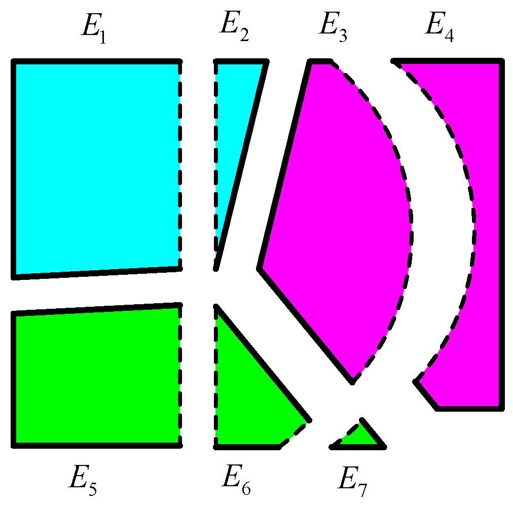
To clarify, a simple example is presented to illustrate the process of constructing the NMM cover system. Figure 2a shows a problem domain $\mathsf{\Omega }$ is subdivided into three separate blocks, i.e., ${\mathsf{\Omega }}_1$, ${\mathsf{\Omega }}_2$ and ${\mathsf{\Omega }}_3$, by its physical meshes. To discretize $\mathsf{\Omega }$, two MCs, i.e., $M_1$ and $M_2$ in Figure 2b, are generated to completely cover $\mathsf{\Omega }$. Then, $M_1$ is subdivided into three PCs, termed as $P_1^1$, $P_1^2$ and $P_1^3$ (Figure 3a), whereas $M_2$ is subdivided into three PCs, termed as $P_2^1$, $P_2^2$ and $P_2^3$ (Figure 3b), by the physical meshes. The six PCs partly overlap each other and cut $\mathsf{\Omega }$ into seven MEs, as shown in Figure 4.

Following generating the cover system, a partition of unity function (weight function) ${\omega }_i\left(x\right)$ and a polynomial local field function are constructed for each PC [41]. Then, the global approximation of the field function in consideration is established by weight averaging the local field functions:

$$X\left(x\right)={\displaystyle \sum _{i=1}^N{\omega }_i\left(x\right)P^{T}a}$$

(1)

where x is the position vector, N is the total number of the PC; $P^T$ represents the polynomial basis vector and a is the corresponding degree of freedom vector of the PC. In this study, the 0th-order polynomial local function is adopted to approximate the local field function. Thus, the global displacement field is written as:

$$u^h\left(x\right)={\displaystyle \sum _{i=1}^N{\omega }_i\left(x\right)\left[\begin{array}{cc}1& 0\\ 0& 1\end{array}\right]d}=N_{u}d$$

(2)

where d is the displacement degree of freedom vector and $N_u$ is the displacement shape function. Similarly, the global temperature field can be written as:

$${\theta }^h\left(x\right)={\displaystyle \sum _{i=1}^N{\omega }_i\left(x\right)\mathsf{\theta }}=N_{\theta }\mathsf{\theta }$$

(3)

where θ is the temperature degree of freedom vector and $N_{\theta }$ is the temperature shape function.

2.1.2. Contact Theory

The NMM inherits the contact theory from DDA to deal with block movements and block interactions [19]. To avoid large displacements in a single time step, a maximum permissible displacement $d_0$ is prescribed in the NMM. Generally, the contact detection process of the NMM can be divided into two separate steps. The first step is detecting the possible contact pairs. The block pair is considered as a possible contact pair if the minimum distance between two blocks is no more than $2d_0$. Basically, three types of contact are defined in the NMM after possible contact detection, i.e., the angle-to-edge contact, the edge-to-edge contact and the angle-to-angle contact, as shown in Figure 5a–c, respectively.

The second step is the invasion judgement of the possible contact pairs. Figure 6 shows when invasion exists in a possible contact pair, one or two point-edge pair are used to completely represent the invasion status of the possible contact pair. To be specific, for angle-to-edge contact and angle-to-angle contact, one point-edge pair can be found, e.g., $V_1$-$V_2{V}_3$ in Figure 6a,c. However, for edge-to-edge contact, two point-edge pairs should be specified to completely represent invasion status, e.g., the $V_1$-$V_3{V}_4$ and $V_2$-$V_3{V}_4$ in Figure 6b. After determining the invasion status of each possible contact pair, the normal invasion displacement $\mathsf{\Delta }o$ and the tangential invasion displacement $\mathsf{\Delta }s$ can be calculated according to the relative position of the corresponding point-edge pair. In NMM, linear elastic contact force–invasion displacement relationships are adopted. Thus the normal contact force and tangential contact force are calculated according to following equations [19]:

$$F_n=k_n\mathsf{\Delta }o\mathsf{\Delta }o<0$$

(4)

$$\{\begin{array}{ll}{F}_s=k_s\mathsf{\Delta }s& F_s\le F_n\tan \phi \\ F_s=F_n\tan \phi & F_s>F_n\tan \phi \end{array}$$

(5)

where $F_n$ and $F_s$ are the normal contact force and the tangential contact force, respectively. $k_n$ and $k_s$ are the corresponding normal contact stiffness and tangential contact stiffness, respectively. The selection of normal and tangential stiffness can greatly influence the output of the numerical model. According to Shi’s suggestion, the ratio of the contact stiffness to the elastic modulus of the block is preferably between 20 and 100 [19].

2.2. Thermal Conduction of Granular Materials

2.2.1. Representation of the Micro Structure of Granular Materials

To more realistically model the thermo-elastic fracturing of the rocklike granular materials, the microstructure of these materials should be considered. The microstructure of the rocklike granular materials appear much like random polygons, as shown in Figure 7a [40]. The Voronoi tessellation is introduced into the pre-processor of the NMM to represent the randomness of the microstructure of granular materials [42]. The Voronoi tessellation begins with generating a set of random points. These random points can be moved step-by-step through an iteration procedure to make the space between the points more uniform. Then triangulation is carried out based on these random points. Following that, the Voronoi polygons are generated by constructing the perpendicular bisectors of all the triangle edges. Finally, by truncating the Voronoi polygons at the boundaries, the random microstructure of granular material is established (Figure 7b). The random microstructure is then treated as the physical meshes of the NMM pre-processor, and the NMM model for granular material finally is constructed by the pre-processor of the NMM (Figure 7c).

2.2.2. Basic Formulas

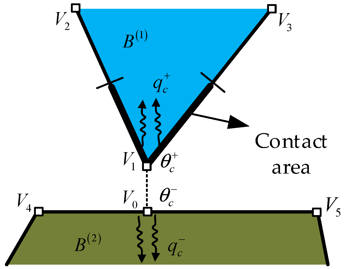
Basically, the thermal conduction of granular materials can be divided into two separate processes, i.e., the heat conduction of solid grains and the heat interactives among bonded grains [7]. The authors consider, without loss of generality, the simple example shown in Figure 8, in which the schematic of the thermal conduction of a granular material consists of two separate grains, ${\mathsf{\Omega }}_1$ and ${\mathsf{\Omega }}_2$, are presented. Figure 8 shows that except for the heat conduction in ${\mathsf{\Omega }}_1$ and ${\mathsf{\Omega }}_2,$ respectively, the heat transferred through the cemented interface ${\mathrm{\Gamma }}_c$ can also dramatically influence the temperature field of the granular material. Thus, apart from the prescribed temperature boundary condition on ${\mathrm{\Gamma }}_{\theta }$ and the prescribed heat flux boundary condition on ${\mathrm{\Gamma }}_q$, the interface heat interactive condition at ${\mathrm{\Gamma }}_c$ should also be satisfied. Considering this, the basic formulas for thermal conduction of granular materials are given as follows:

• The first law of thermodynamics

  $$\nabla q\left(x,t\right)+\rho c_{\theta }\frac{\partial {\theta }^h\left(x,t\right)}{\partial t}=Q$$

  (6)
• Fourier’s law

  $$q\left(x,t\right)=-k\nabla {\theta }^h\left(x,t\right)$$

  (7)

  where $\rho$ is the mass density, $q\left(x,t\right)$ is the heat flux, $c_{\theta }$ is the specific heat, Q is the heat source per unit area, k is the thermal conductivity of the solid grains, $\nabla$ is the gradient operator. Correspondently, the boundary and initial conditions for thermal conduction are given as follows:
• Boundary conditions

  $${\theta }^h\left(x,t\right)=\overline{\theta }\left(x,t\right)\mathrm{on}{\mathrm{\Gamma }}_{\theta }$$

  (8)

  $$q\left(x,t\right)\cdot n=\overline{q}\left(x,t\right)\mathrm{on}{\mathrm{\Gamma }}_q$$

  (9)
• Initial conditions

  $${\theta }^h\left(x,0\right)={\theta }_0$$

  (10)

  where n is the outside unit normal vector. ${\mathrm{\Gamma }}_{\theta }$, ${\mathrm{\Gamma }}_q$ are the boundaries with prescribed temperature $\overline{\theta }$ and prescribed heat flux $\overline{q}$, respectively. ${\theta }_0$ represents initial temperature of the problem domain. Moreover, the solution of temperature field should also satisfy the interface heat interactive conditions:

  $$q\left(x,t\right)\cdot n^{+}=q_c^{+}\mathrm{on}{\mathrm{\Gamma }}_c^{+}$$

  (11)

  $$q\left(x,t\right)\cdot n^{-}=q_c^{-}\mathrm{on}{\mathrm{\Gamma }}_c^{-}$$

  (12)

  where $n^{+}$ and $n^{-}$ denote the corresponding outside unit normal vector of the upper boundary ${\mathrm{\Gamma }}_c^{+}$ and lower boundary ${\mathrm{\Gamma }}_c^{-}$, respectively. $q_c^{+}$ and $q_c^{-}$ represent the amount of heat flux across the boundary ${\mathrm{\Gamma }}_c^{+}$ and ${\mathrm{\Gamma }}_c^{-}$, respectively.

2.2.3. Contact Based Heat Transfer Model

To obtain the temperature field of the granular material from the basic formulas presented above, the amount of the heat flux transferred through the cemented interfaces should be prescribed first. Inspired from the fact that the NMM adopts contact algorithm to deal with the interactions between blocks, a contact based heat transfer model is developed to simulate the heat interactive among grains in this study. The heat interactive between the two grains are considered only when the two grains are cemented together or contact each other. Since the contact status of a possible contact can be completely represented by the geometric relation of corresponding point-edge relations, the contact-based heat transfer model in this study is also based on the point-edge relations. Additionally, according to Fourier’s law, the amount of the heat flux transferred across the interface depends on the heat conduction capacity of the interface. Thus, in the rest of this article, a contact thermal conductivity $k_c$ is defined to represent the heat conduction capacity of the interface. The physical meaning of $k_c$ is the amount of heat flux transferred across unit length of interface per unit time in case of unit temperature difference. The heat conduction capacity of the cemented interfaces might be related to many factors, such as the contact force, the roughness of the interface and the hardness of the material [43,44]. However, this is not the main research objective of this work.

To explain the contact-based heat transfer model in detail, a representative example is shown in Figure 9, in which block $B^{\left(1\right)}$ contacts block $B^{\left(2\right)}$ at point $V_1$ of $B^{\left(1\right)}$ and point $V_0$ of $B^{\left(2\right)}$ respectively. The contact status of this contact pair is represented with the point-edge relation $V_1$-$V_4{V}_5$. The heat interactive between $B^{\left(1\right)}$ and $B^{\left(2\right)}$ is then approximated by the heat interactive between boundary $V_4{V}_5$ and point $V_1$.

As the thickness and the volume of the interfaces are not explicitly represented in the NMM. The cemented interfaces are assumed to be with zero thickness and zero volume. Based on this kind of treatment, it is supposed that the cemented interface between blocks have no heat storage capacity and ignoring the frictional heat. Thus, the following balance equation of the heat flux at the interface is thus obtained:

$$q_c^{+}=-q_c^{-}=q_c$$

(13)

According to Fourier’s law, the amount of heat flux transferred through the interface is related to the contact thermal conductivity, the interface temperature difference as well as the contact area. Thus, the amount of interface heat flux can be written as:

$$q_c\left(x,t\right)=-k_{c}l\mathsf{\Delta }{\theta }_c\left(x,t\right)$$

(14)

with l representing the contact area as shown in Figure 9:

$$l=\frac{1}{2}\left(\Vert x_1-x_2\Vert +\Vert x_1-x_3\Vert \right)$$

(15)

where $x_1$, $x_2$ and $x_3$ are the position vectors of $V_1$, $V_2$ and $V_3$ respectively. $\mathsf{\Delta }{\theta }_c$ in Equation (14) represents the temperature difference between $V_4{V}_5$ and $V_1$, which is approximated by the temperature difference between $V_1$ and the projection point $V_0$ as shown in Figure 9:

$$\mathsf{\Delta }{\theta }_c={\theta }_c^{+}-{\theta }_c^{-}$$

(16)

where ${\theta }_c^{+}$ and ${\theta }_c^{-}$ represent the temperatures at point $V_1$ and $V_0$, respectively, which can be approximated by the linear interpolation of the corresponding PC temperatures:

$${\theta }_c^j=\left[\begin{array}{ccc}{N}_1^j& N_2^j& N_3^j\end{array}\right]\left\{\begin{array}{c}{\theta }_1^j\\ {\theta }_2^j\\ {\theta }_3^j\end{array}\right\}=N_{\theta }^j\mathsf{\theta },j=+\mathrm{or}-$$

(17)

Thus, Equation (16) can be shortened as:

$$\mathsf{\Delta }{\theta }_c=\left[\begin{array}{cc}{N}_{\theta }^{+}& -N_{\theta }^{-}\end{array}\right]\cdot \mathsf{\theta }=N_{\theta }^c\mathsf{\theta }$$

(18)

2.2.4. Discretization and Solution

To obtain the temperature field of the granular material, the governing equation should be established by discretizing the basic formulas described in Section 2.2.2 and the contact-based heat transfer model in Section 2.2.3. In this section, the weight residual method is adopted to establish the governing equation [41]. The weak form of the governing equation can be expressed as:

$$\begin{array}{l}{\displaystyle {\int }_{\mathsf{\Omega }}\delta {\theta }^h\cdot \rho c_{\theta }\frac{\partial {\theta }^h}{\partial t}d\mathsf{\Omega }}+{\displaystyle {\int }_{\mathsf{\Omega }}\frac{1}{k}\left[q_x\left(\delta {\theta }^h\right)q_x\left({\theta }^h\right)+q_y\left(\delta {\theta }^h\right)q_y\left({\theta }^h\right)\right]d\mathsf{\Omega }}\\ +{\displaystyle {\int }_{{\mathrm{\Gamma }}_{\theta }}\delta {\theta }^h\cdot {\lambda }_T\left({\theta }^h-\overline{\theta }\right)d\mathrm{\Gamma }}={\displaystyle {\int }_{{\mathrm{\Gamma }}_q}\delta {\theta }^h\cdot \overline{q}d\mathrm{\Gamma }}+{\displaystyle \underset{\mathrm{contact}}{\cup }\left(\delta {\theta }^{+}{q}_c^{+}+\delta {\theta }^{-}{q}_c^{-}\right)}\end{array}$$

(19)

where $\mathsf{\delta }{\theta }^h$ is the first order variation of ${\theta }^h\left(x,t\right)$ and ${\lambda }_T$ is the penalty number to enforce the prescribed temperature boundary condition. The last term in Equation (19) is the contact heat transfer terms which have to satisfy the heat flux continuity condition given in Equation (13) and the temperature condition given in Equation (16). By substituting Equation (14) and (18) into Equation (19), the discretized governing equation for transient heat conduction with contact heat transfer among cemented grains can be established:

$$C_{\theta }\dot{\mathsf{\theta }}+K_{\theta }\mathsf{\theta }=F_{\theta }$$

(20)

where:

$$C_{\theta }=\rho c_{\theta }{\displaystyle {\int }_{\mathsf{\Omega }}{N}_{\theta }^T{N}_{\theta }d\mathsf{\Omega }}$$

(21)

$$\begin{array}{l}{K}_{\theta }={\displaystyle {\int }_{\mathsf{\Omega }}\left[k{\left(\frac{\partial N_{\theta }}{\partial x}\right)}^T\left(\frac{\partial N_{\theta }}{\partial x}\right)+k{\left(\frac{\partial N_{\theta }}{\partial y}\right)}^T\left(\frac{\partial N_{\theta }}{\partial y}\right)\right]d\mathsf{\Omega }}\\ +{\lambda }_T{\displaystyle {\int }_{{\mathrm{\Gamma }}_{\theta }}{N}_{\theta }^T{N}_{\theta }d{\mathrm{\Gamma }}_{\theta }}+{\displaystyle \underset{\mathrm{contact}}{\cup }{\left(N_{\theta }^c\right)}^T\cdot k_{c}l\cdot N_{\theta }^c}\end{array}$$

(22)

$$F_{\theta }={\lambda }_T{\displaystyle {\int }_{{\mathrm{\Gamma }}_{\theta }}{N}_{\theta }^T\overline{\theta }d{\mathrm{\Gamma }}_{\theta }}-{\displaystyle {\int }_{{\mathrm{\Gamma }}_q}{N}_{\theta }^T\overline{q}d{\mathrm{\Gamma }}_q}$$

(23)

Equation (20) is a first-order time dependent differential equation, which can be solved by the time integration scheme [45]. Generally, the time integration scheme for transient heat conduction can be uniformly written as:

$$\{\begin{array}{l}{\mathsf{\theta }}^{k+1}={\mathsf{\theta }}^k+\left[\left(1-\beta \right){\dot{\mathsf{\theta }}}^k+\beta {\dot{\mathsf{\theta }}}^{k+1}\right]\mathsf{\Delta }{t}^{k+1}\\ C_{\theta }\frac{{\mathsf{\theta }}^{k+1}-{\mathsf{\theta }}^k}{\mathsf{\Delta }{t}^{k+1}}+K_{\theta }\left[\left(1-\beta \right){\mathsf{\theta }}^k+\beta {\mathsf{\theta }}^{k+1}\right]=\left(1-\beta \right)F_{\theta }^k+\beta F_{\theta }^{k+1}\end{array}$$

(24)

in which, k is the serial number of the time step, $\mathsf{\Delta }{t}^{k+1}=t^{k+1}-t^k$ is the time interval of the k + 1 time step, ${\mathsf{\theta }}^k$ and ${\mathsf{\theta }}^{k+1}$ are the temperature degree of freedom vectors of the k time step and the k + 1 time step respectively. The parameter $\beta$ is adopted to choose the specific time integration scheme. Regarding $1/2\le \beta \le 1$, the time integration scheme is unconditionally stable [45]. In this study, $\beta =1$ is adopted to solve the governing equation as it is unconditionally stable and relatively easy to be implemented into NMM. Thus, Equation (32) can be simplified as:

$$\left(K_{\theta }+\frac{C_{\theta }}{\mathsf{\Delta }{t}^{k+1}}\right){\mathsf{\theta }}^{k+1}=F_{\theta }^{k+1}+\frac{C_{\theta }}{\mathsf{\Delta }{t}^{k+1}}{\mathsf{\theta }}^k$$

(25)

2.3. Thermo-Elastic Fracture Analysis

2.3.1. Thermo-Mechanical Coupling

The variation of temperature can lead to thermal expansion or thermal shrinkage of materials. As materials are generally under different external constrains, the thermal expansion or shrinkage of the materials cannot occur freely in all directions. Subsequently, thermal stresses and even thermal fractures usually appears in the materials. The thermal induced stress can be written as:

$${\mathsf{\sigma }}_{\theta }=-D{\mathsf{\epsilon }}_{\theta }=-D\cdot \alpha \mathsf{\Delta }{\theta }^{h}I$$

(26)

where ${\mathsf{\sigma }}_{\theta }$ and ${\mathsf{\epsilon }}_{\theta }$ are the thermal induced stress and strain vector respectively, $\mathsf{\Delta }{\theta }^h$ is the amount of temperature variation, α represents the thermal expansion coefficient, D is the linear elastic constitutive matrix and I is the second order identity tensor. The thermal induced stress can be easily incorporated into the NMM by treating ${\mathsf{\sigma }}_{\theta }$ as the initial stress of the NMM [38].

2.3.2. A Damage Based Contact Fracture Model

The micrograins of granular materials in Nature are bonded together by the cemented interface. However, the cohesion effects among blocks are neglected in the original contact algorithm of the NMM. Additionally, under thermal circumstances, the thermal induced stresses could result in fracture evolution in the granular materials. Thus, the contact algorithm of the NMM should be improved to successfully simulate the cohesion effects and the thermal fracture evolution of the granular materials. To achieve this goal, a damage-based contact fracture model is incorporated into the NMM in this study [46].

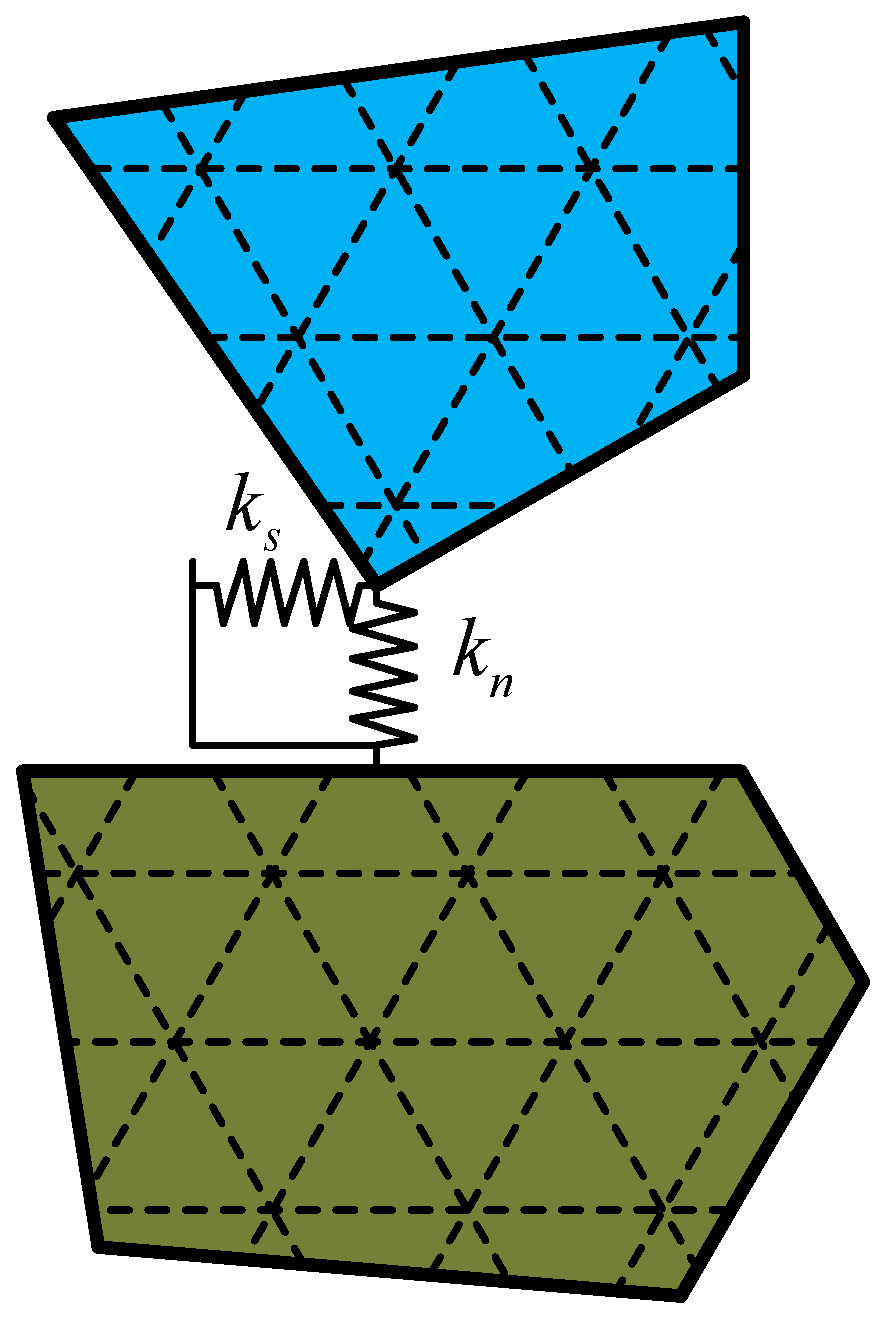
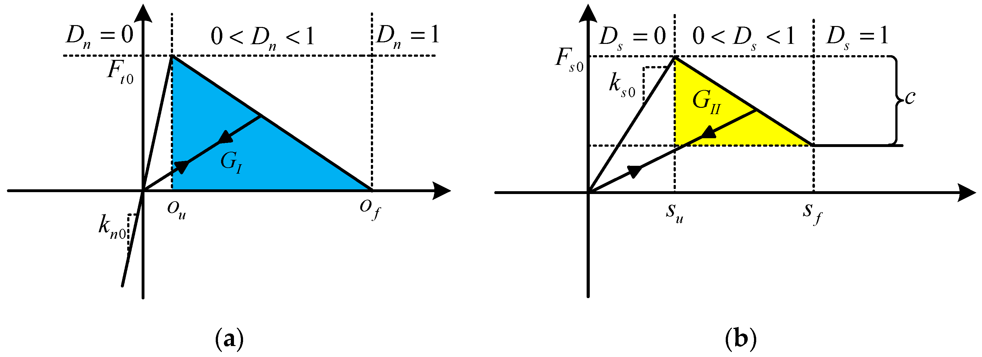
As mentioned in Section 2.1.2, after the invasion judgement, the invasion status of contact block pairs are obtained. Generally, the interactions among grains are divided into normal behavior and tangential behavior. In NMM, normal contact springs and tangential contact springs are adopted to simulate the normal behaviors and tangential behaviors among blocks as shown in Figure 10. To be consistent with this and to simulate the cohesion effects among blocks as well, the normal force-aperture relationship shown in Figure 11a and the tangential force-aperture relationship shown in Figure 11b are adopted and assigned to the normal spring and tangential spring respectively. Correspondently, to reflect the damage evolution process of the cemented interface, two damage factors, i.e., the normal damage factor $D_n$ and the tangential damage factor $D_s$, are defined for the normal contact spring and tangential contact spring respectively. The normal behavior and tangential behavior of the damage based contact fracture model are described in detail as follows.

As shown in Figure 11a, the normal behavior of the contact is divided into three parts according to the normal damage factor. The normal damage factor can be calculated by the following formula:

$$D_n=\{\begin{array}{ll}0& o\le o_u\\ \frac{o-o_u}{o_f-o_u}& o_u<o\le o_f\\ 1& o>o_f\end{array}$$

(27)

where o is normal aperture, $o_u$ and $o_f$ represent the normal aperture corresponding to the initial tensile strength of the contact $F_{t0}$ and the tensile failure of the contact, respectively:

$$o_u=\frac{F_{t0}}{k_{n0}}$$

(28)

$$o_f=o_u+\frac{2G_I}{F_{t0}}$$

(29)

where $k_{n0}$ is the initial stiffness of the normal spring and $G_I$ represents the mode I critical energy release rate. The tensile strength of the contact $F_{t0}$ can be determined by $F_{t0}=l{f}_{t0}$, in which l is the contact area defined in Figure 9 and $f_{t0}$ is the initial tensile strength of the interface per unit length.

Based on the above descriptions, the normal force of the damage based contact fracture model can be expressed as follows:

$$F_n=\{\begin{array}{ll}{k}_{n0}o& o\le o_u\\ \left(1-D_n\right)F_{t0}& o_u<o\le o_f\\ 0& o>o_f\end{array}$$

(30)

Similar to the normal behavior, the tangential behavior of the contact is also divided into three parts according to the tangential damage factor (Figure 11b). The tangential damage factor can also be calculated according to the tangential aperture:

$$D_s=\{\begin{array}{ll}0& s\le s_u\\ \frac{s-s_u}{s_f-s_u}& s_u<s\le s_f\\ 1& s>s_f\end{array}$$

(31)

where s represents the tangential aperture of the contact. $s_u$ and $s_f$ are the tangential apertures corresponding to the initial shear strength of the contact $F_{s0}$ and the shear failure of the contact respectively, which can be calculated as follows:

$$s_u=\frac{F_{s0}}{k_{s0}}$$

(32)

$$s_f=s_u+\frac{2G_{II}}{c}$$

(33)

where $G_{II}$ denotes the mode II critical energy release rate; c represents the initial cohesion of the contact; $k_{s0}$ is the initial stiffness of the tangential spring. According to Coulomb’s friction law, the initial shear strength $F_{s0}$ of the contact can be written as:

$$F_{s0}=F_n\tan \phi +c$$

(34)

where φ is the internal friction angle of the contact. As the cohesion of the contact decreases linearly with the increase of tangential damage factor as shown in Figure 11b, the tangential contact force-aperture relationship can thus be expressed as:

$$F_s=\{\begin{array}{ll}{k}_{s0}s& s\le s_u\\ F_n\tan \phi +\left(1-D_s\right)c& s_u<s\le s_f\\ F_n\tan \phi & s>s_f\end{array}$$

(35)

Furthermore, to distinguish the mode I fracture, the mode II fracture and the mixed mode fracture as well as judge the failure of the cemented interface, a mixed mode damage factor is defined. The mixed mode damage factor is calculated by the following equation:

$$D_{mix}=\sqrt{{\left(D_n\right)}^2+{\left(D_s\right)}^2}$$

(36)

It is supposed that whenever the mixed damage factor exceeds 1, the contact is set as “failure”.

3. Results and Discussion

3.1. Validation of Contact Heat Transfer Model

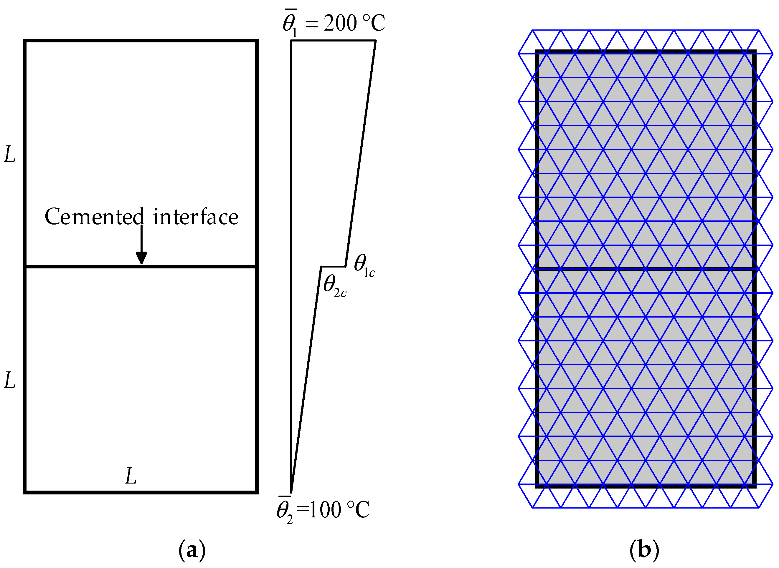
The thermal conduction in a plane consists of two square blocks is simulated in this example to verify the effectiveness of the developed contact heat transfer model. The edge length of the square blocks is L = 1.5 mm. The plane is subjected to prescribed temperature conditions on the top boundary and bottom boundary, as shown in Figure 12a. The two blocks are bonded together by the center cemented interface. The heat transfer across the cemented interface should influence the temperatures on the two sides of the cemented interface, which is termed as ${\theta }_{1c}$ and ${\theta }_{2c}$ in this example. The steady state theoretical solutions for ${\theta }_{1c}$ and ${\theta }_{2c}$ can be calculated according to the following equations [43]:

$${\theta }_{1c}=\frac{\left(1+\eta \right){\overline{\theta }}_1+\eta {\overline{\theta }}_2}{1+2\eta }$$

(37)

$${\theta }_{2c}=\frac{\eta {\overline{\theta }}_1+\left(1+\eta \right){\overline{\theta }}_2}{1+2\eta }$$

(38)

where η indicates the ratio of the contact thermal conductivity to the material thermal conductivity:

$$\eta =\frac{k_c}{k}$$

(39)

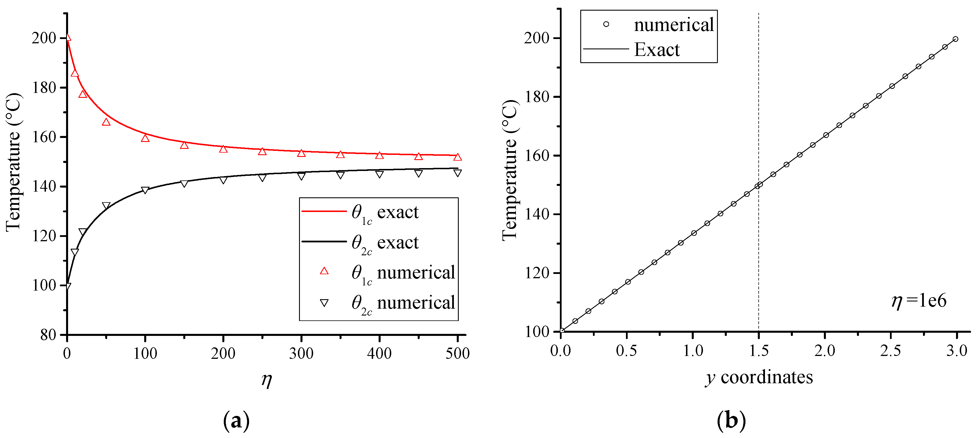
The NMM cover system shown in Figure 12b is constructed to implement the numerical simulation. The numerical results of ${\theta }_{1c}$ and ${\theta }_{2c}$ for cases with different η are compared with the corresponding theoretical solutions in Figure 13a, which indicates good agreements. Moreover, it is illustrated in Figure 13 that the temperature difference at the cemented interface decreases with the increase of η. Therefore, it is inferred that when η is large enough, the interface temperature difference would diminish to 0. To validate this point of view, Figure 13b shows the temperature on the center vertical line of the plane for case with η = 1 × 10⁶. Obviously, the temperature agrees well with the exact temperature solution of a continuous plane with the same size and boundary conditions.

3.2. Validation of Thermo-Mechanical Coupling

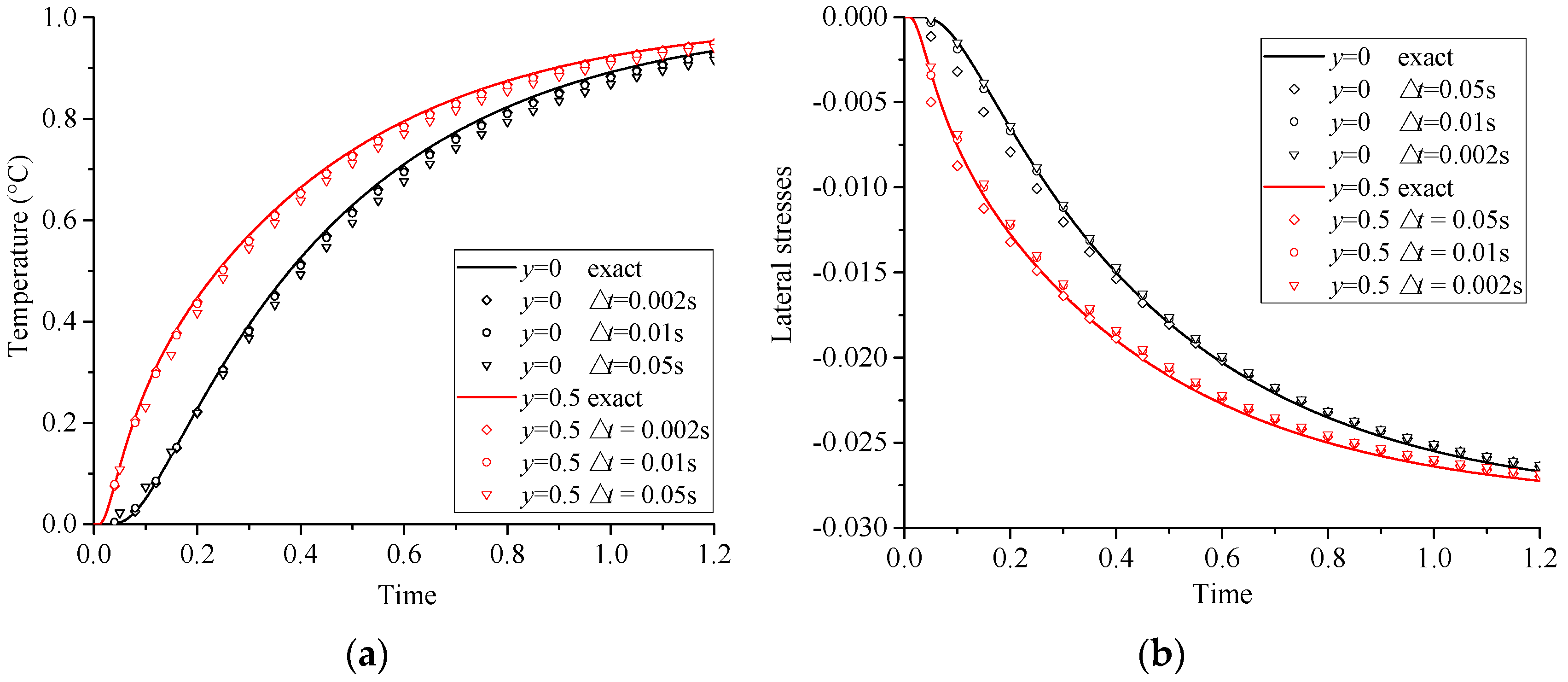
A simple thermo-mechanical coupling problem is analyzed to validate effectiveness of the extended NMM on simulating thermo-mechanical coupling problems. As shown in Figure 14a, a square plane with edge length L = 1 m and initial temperature ${\theta }_0=0 °\mathrm{C}$ is subjected to thermal loading ${\overline{\theta }}_1=1 °\mathrm{C}$ on the top boundary. The vertical displacement of the bottom boundary as well as the horizontal displacements of the right boundary and left boundary are fixed. The plane is subjected to plane strain conditions.

According to thermodynamics, the heat flux would flow gradually from the top boundary to the bottom boundary. The resulting temperature variation could cause thermal expansion and thermal stresses in the plane. To investigate these phenomenon, this transient heat transfer process is numerically simulated by the extended NMM. The variation of the temperatures and lateral stresses at point A (0.5, 0) and point B (0.5, 0.5) with time for cases with different time step sizes are extracted and investigated as shown in Figure 15a,b. To compare, the corresponding theoretical solutions for the temperatures and stresses are obtained according to the following equations [47]:

$$\{\begin{array}{l}\theta \left(y,t\right)=1-\frac{4}{\pi }{\displaystyle \sum _{n=0}^{\infty }\frac{{\left(-1\right)}^n}{2n+1}\exp \left[-\frac{\left(2n+1\right){\pi }^{2}kt}{4L^2\rho c_{\theta }}\right]\cos \left[\frac{\left(2n+1\right)\pi y}{2L}\right]}\\ {\sigma }_x=-\frac{\alpha E}{1-\mu }\theta \left(y,t\right)\end{array}$$

(40)

It is clearly indicated in the figure that good agreements between the numerical results and theoretical solutions are obtained, which confirms the effectiveness of the extended NMM on simulating thermo-mechanical coupling problems. Moreover, the figures illustrate that the numerical results are more accurate for smaller time step size, e.g., $\mathsf{\Delta }t=0.002\mathrm{s}$ in Figure 15.

3.3. Thermo-Elastic Fracturing Induced by Elevated Temperature

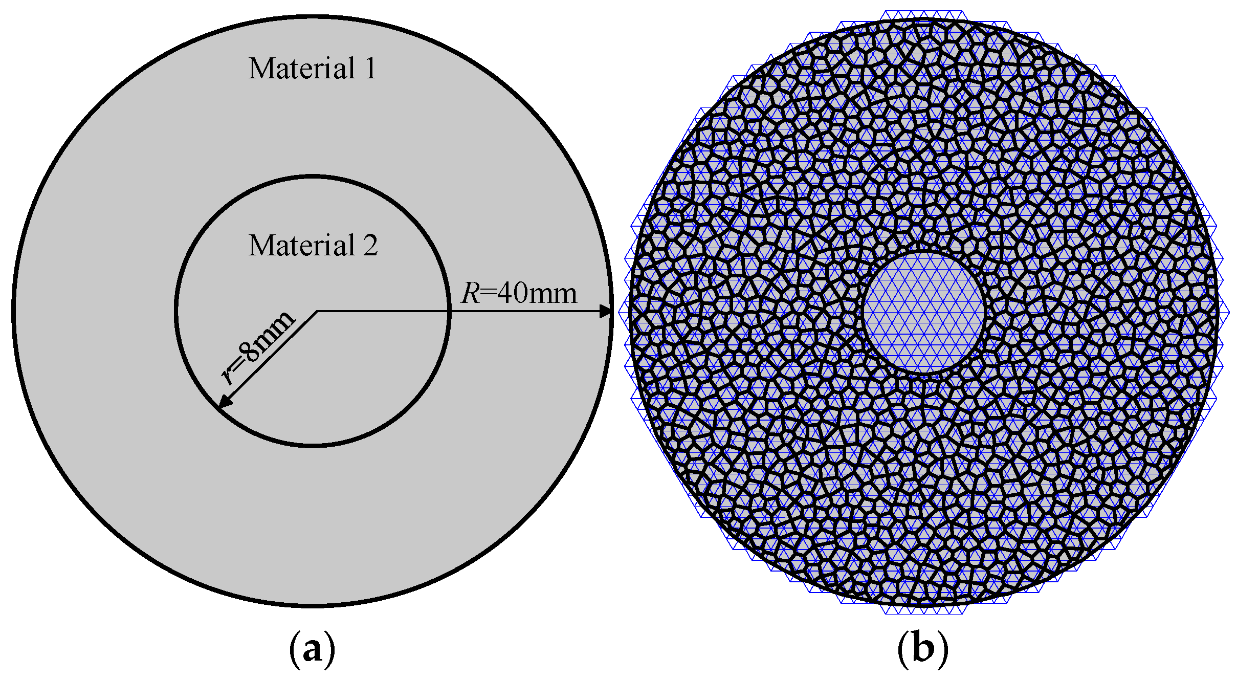
The thermo-elastic fracturing of a model consists of an outer cylinder and an inner disc is numerically investigated in this example. The radii of the cylinder and the disc are shown in Figure 16a. The initial temperature of the model is $0 °\mathrm{C}$. The cylinder and disc are made of two different materials respectively, termed as Material 1 and Material 2 as shown in Figure 16a, where Material 1 is supposed to be a typical granular material. The temperature of the model is supposed to be increased uniformly, in which condition only the thermal fracturing process is considered and the heat transfer across the model can be ignored. The material parameters of Material 1 and Material 2 are presented in

Table 1. Parameters for Example 3.

Parameters	Material 1	Material 2
Material
Bulk density, $\rho$ ($\mathrm{kg}/{\mathrm{m}}^3$)	2300	2300
Elastic modulus, E (GPa)	20	40
Poisson’s ratio, μ	0.3	0.3
Thermal expansion, α [48]	1 × 10−6	1.5 × 10−6
Interface
Contact thermal conductivity, $k_c$($\mathrm{W}/\left(\mathrm{m}·℃\right)$)	1 × 108
Initial temperature, ${\theta }_0 (℃)$	0
Normal contact stiffness, $k_n$	1 × 107
Tangential contact stiffness, $k_s$	4 × 106
Cohesion, $c\left(\mathrm{MPa}\right)$	10
Tensile strength, $f_{t0} \left(\mathrm{MPa}\right)$	5
Friction angle, $\phi (°)$	0
Mode I energy release rate, $G_I \left(\mathrm{J}/{\mathrm{m}}^2\right)$	40
Mode II energy release rate, $G_{II} \left(\mathrm{J}/{\mathrm{m}}^2\right)$	200

. Since the elastic modulus and the thermal expansion coefficient of Material 2 are larger than those of Material 1, thermal fracturing would occur in Material 1 when the temperature of the model is uniformly elevated. To investigate this thermal fracturing process, the cylinder is subdivided into 1241 Voronoi polygons as shown in Figure 16b. The contact-based heat transfer model and the damage-based contact fracture model are used to simulate the heat interactive and the bonding-cracking effects between the micro grains. The parameters of the interface are presented in Table 1 as well.

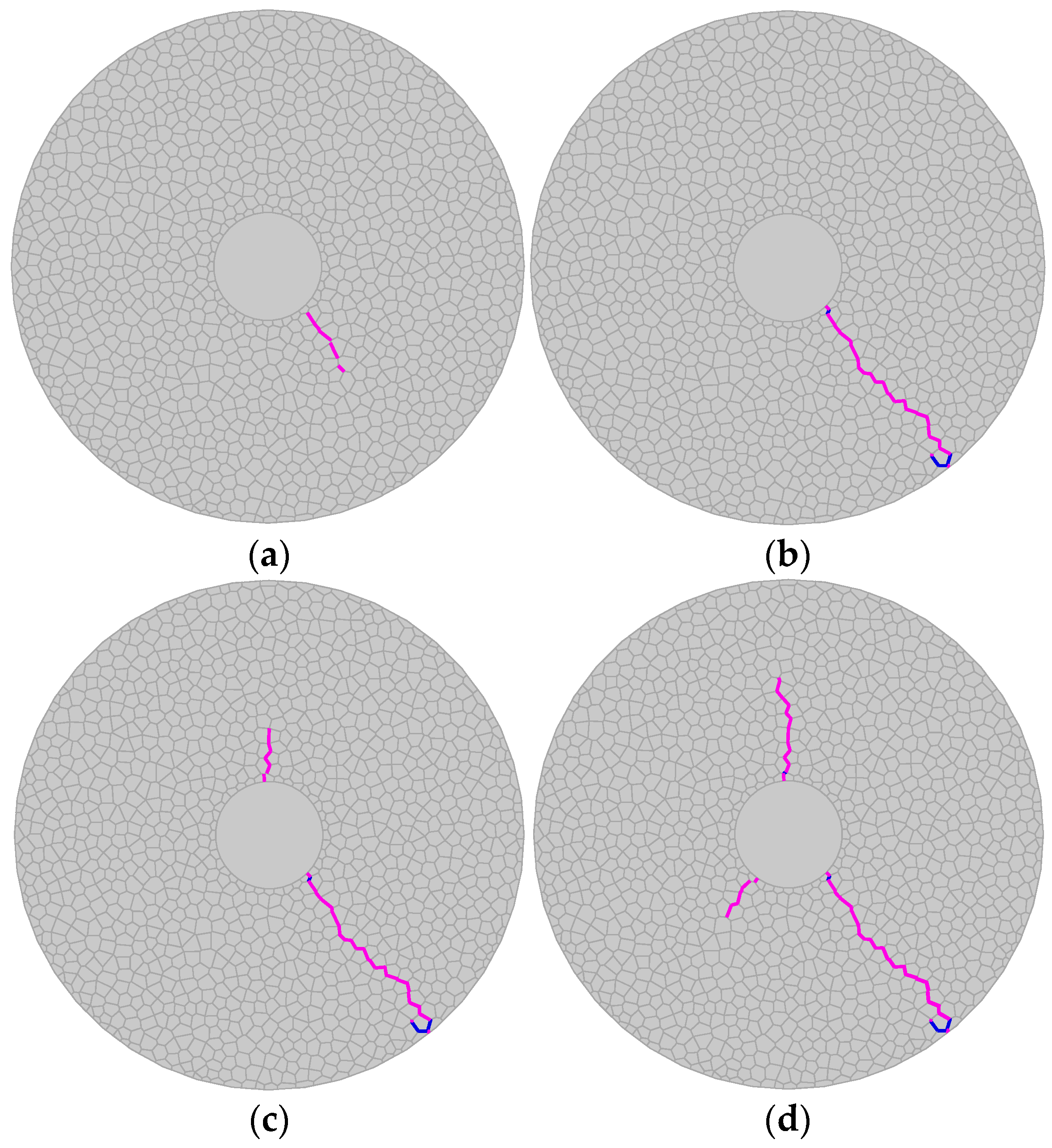
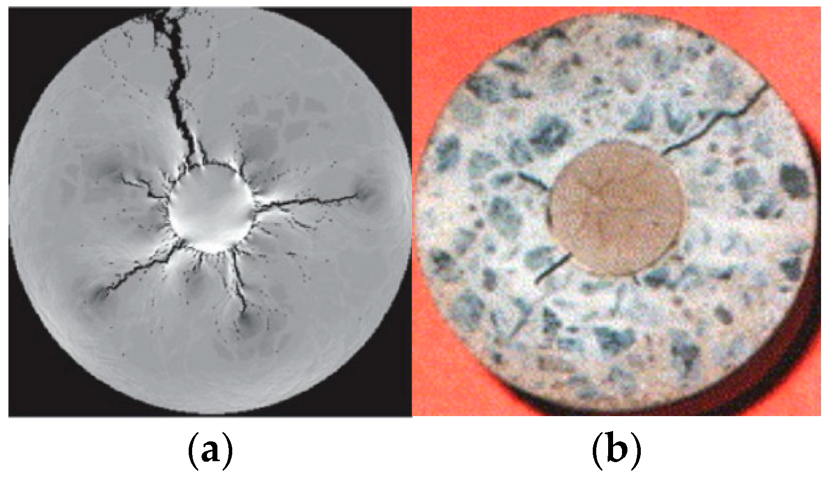
The NMM cover system with 11,187 MEs and 10,955 PCs are generated to simulate this problem (Figure 16b). According to the analysis of Example 2, the time step size adopted for the numerical simulation is $\mathsf{\Delta }t=0.001\mathrm{s}$. During the numerical simulation, the temperature of the model is increased uniformly by $0.3 °\mathrm{C}$ per time step. The numerical results of the thermal fracturing processes are shown in Figure 17. A fracture initiates at the lower right corner of the cylinder first (Figure 17a). This fracture propagates rapidly until it completely cut-through the cylinder at $480 °\mathrm{C}$ (Figure 17b). Subsequently, two secondary fractures initiate at the upper left and lower left corners of the cylinder at $651 °\mathrm{C}$ (Figure 17c) and $750 °\mathrm{C}$ (Figure 17d), respectively. Similar numerical simulation of this example has been conducted by the RFPA-thermal [12]. Figure 18a shows the final thermal fracture morphology of the RFPA-thermal, in which one main radial fracture that cut-through the outer cylinder as well as some shorter secondary radial fractures are also obtained. A similar experiment test has also conducted by Abdalla [49]. In Abdalla’s experiment test, a concrete prism symmetrically reinforced by FRP bars is subjected to uniform rise of temperature. The thermal expansion coefficient of FRP in the test is much larger than that of the concrete. As a result, transverse thermal stresses gradually increase in the concrete, which further leads to the radial fracturing in the concrete surrounding the FRP bars. Figure 18b shows the thermal fracture morphology of the test. Similar to the numerical results, one main radial fracture is initiated and finally cut-through the surrounding concrete. Along with the main fracture, there are also some shorter radial fractures in the surrounding concrete.

3.4. Thermo-Elastic Fracturing Induced by Cooling

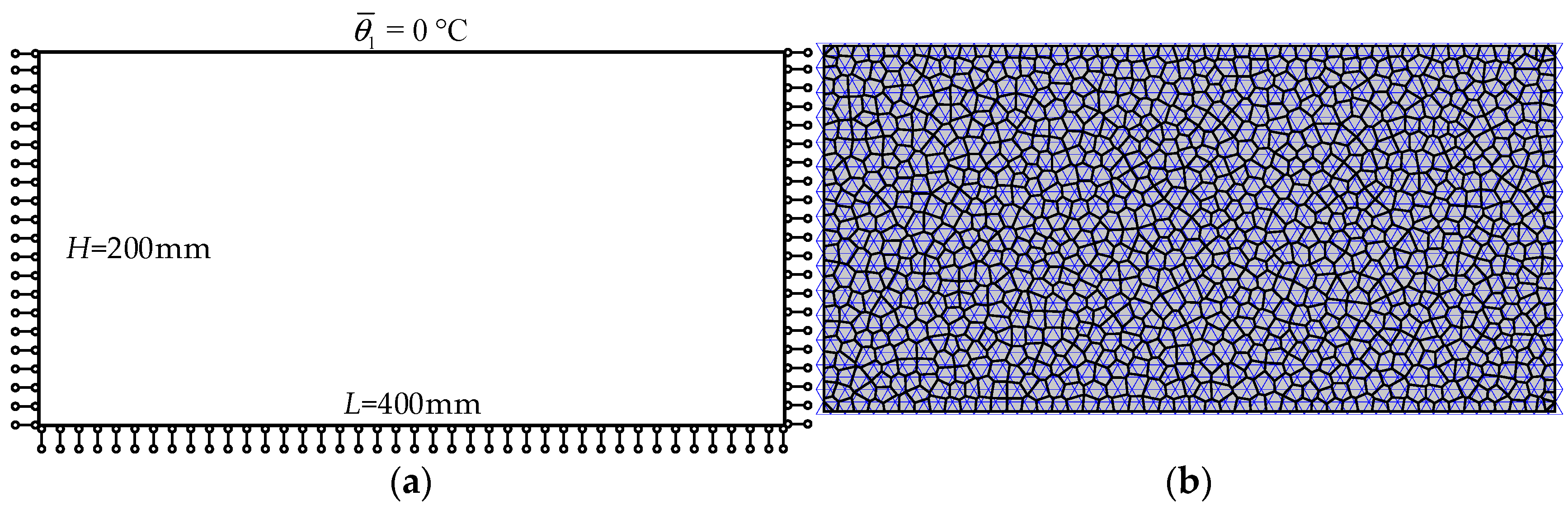
The thermo-elastic fracturing of a plane made of granular material induced by cooling is studied in this example. The length and height of the plane are L = 400 mm and H = 200 mm respectively, as shown in Figure 19a. The vertical displacement of the bottom boundary as well as the horizontal displacements of the left and right boundaries are fixed, while the top boundary is mechanically free. The plane is originally subjected to a high temperature circumstance with initial temperature ${\theta }_0=1000 ℃$. The left, right and bottom boundaries are adiabatic. The top boundary is held at a prescribed temperature of ${\overline{\theta }}_1=0 ℃$ to mimic the contact of the plane with cold, e.g., rapidly flowing cold water.

To simulate this thermal cooling induced fracture evolution, 1022 Voronoi polygons are generated to represent the micro structure of the plane as shown in Figure 19b. Then, the NMM cover system with 8789 MEs, 8754 PCs is constructed based on the Voronoi assemblies. The material parameters and the interface parameters of the numerical simulation are presented in

Table 2. Parameters for Example 4.

Parameters
Material
Bulk density, $\rho$ ($\mathrm{kg}/{\mathrm{m}}^3$)	2500
Elastic modulus, E (GPa)	30
Poisson’s ratio, μ	0.3
Thermal conductivity, $k$($\mathrm{W}/\left(\mathrm{m}·℃\right)$)	3
Specific heat, $c_{\theta }$($\mathrm{J}/\mathrm{kg}·℃$)	1000
Thermal expansion, α	5 × 10−6
Interface
Contact thermal conductivity, $k_c$($\mathrm{W}/\left(\mathrm{m}·℃\right)$)	1 × 105
Initial temperature, ${\theta }_0 (℃)$	1000
Normal contact stiffness, $k_n$	1 × 107
Tangential contact stiffness, $k_s$	4 × 106
Cohesion, $c\left(\mathrm{MPa}\right)$	30
Tensile strength, $f_{t0} \left(\mathrm{MPa}\right)$	10
Friction angle, $\phi (°)$	0
Mode I energy release rate, $G_I \left(\mathrm{J}/{\mathrm{m}}^2\right)$	50
Mode II energy release rate, $G_{II} \left(\mathrm{J}/{\mathrm{m}}^2\right)$	200

.

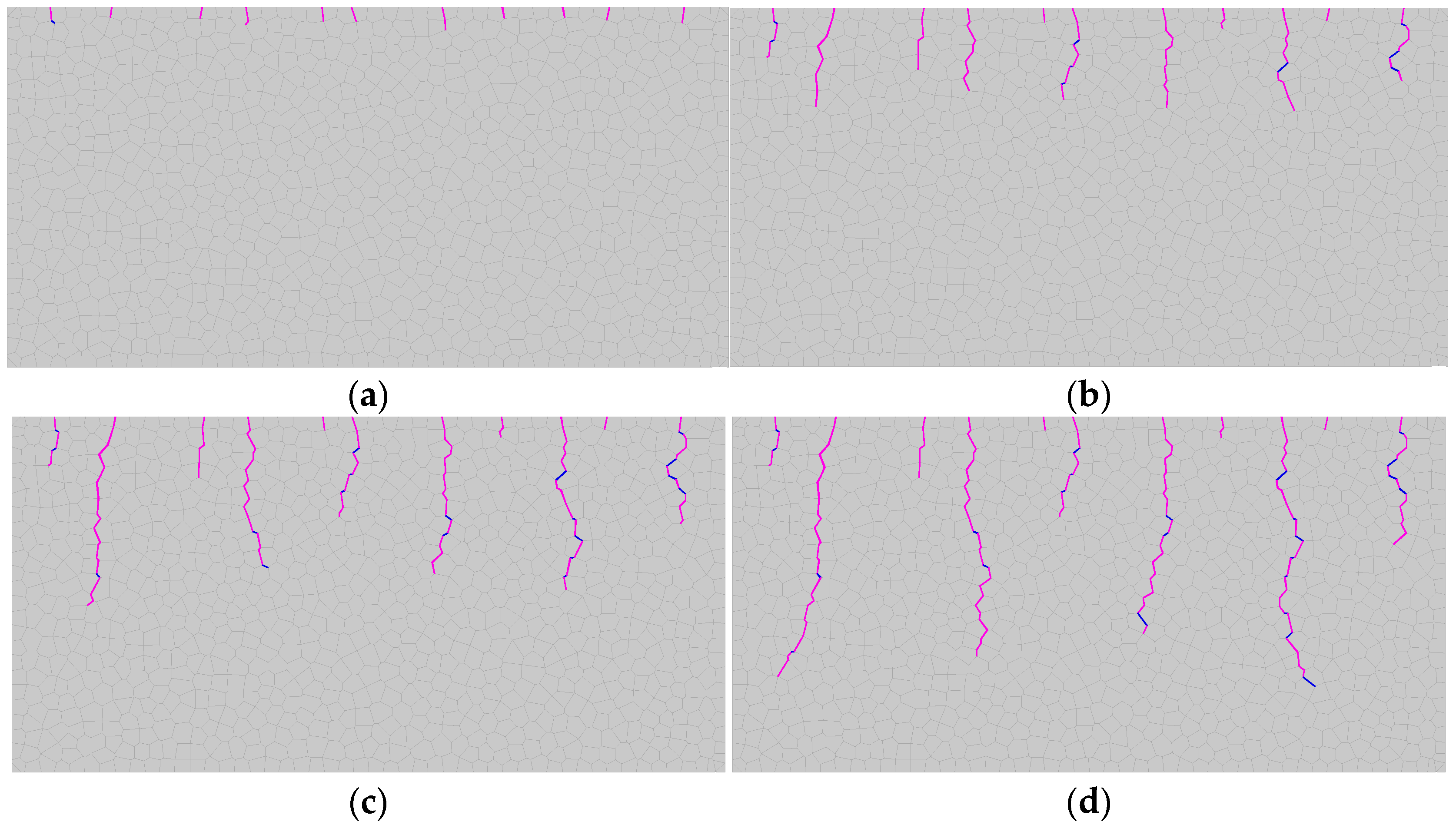
The numerical results of the thermal fracturing process are shown in Figure 20. During the numerical simulation, an array of small fractures emerge at the top boundary of the plane immediately after the cooling process starts, which is due to the large temperature gradient near the top boundary (Figure 20a). These small fractures propagate downwards as the plane cools gradually from the top boundary to the bottom boundary. Additionally, the number of fractures that continue to grow downwards decrease monotonically. Generally, the ultimate thermal fracture patterns are mainly in the vertical direction, which is parallel to the average temperature gradient. However, due to the heterogeneity of the grain structure, the thermal fracture patterns are slightly deviated from the vertical direction. This numerical result is consistent with that obtained by Huang [50].

4. Conclusions

Because of the environmental friendliness and reliable features of geothermal energy, exploration and exploitation of geothermal energy is attracting more and more attention. However, since rocks are typical heterogeneous granular materials, the randomly shaped microstructure of the rock can bring about uncoordinated thermal stresses and even result in thermal fracturing when the deep high temperature circumstance is disturbed during geothermal energy exploitation. The geothermal-related thermal fracturing of rock can significantly influence the geothermal energy exploitation.

In this study, a thermo-mechanical coupling algorithm based on the numerical manifold method was developed to analyze the thermo-elastic fracturing process of granular materials. The developed NMM algorithm represented the randomly shaped microstructure of granular materials using Voronoi polygon assemblies. Based on the Voronoi polygon assembly, a transient thermal conduction algorithm for granular materials was established, in which the heat interactions among Voronoi grains were reflected by a newly developed contact-based heat transfer model. Then, a damage-based contact fracture model was incorporated in the NMM algorithm to simulate the bonding-cracking effects between grains. The newly developed NMM algorithm was validated by two simple examples, the results of which agreed well with that of theoretical solutions. At last, the thermo-elastic fracturing processes induced by elevated temperature and cooling were simulated by the developed NMM algorithm. The obtained thermal fracture morphologies were consistent with those obtained by experiment test and available numerical simulations.

The developed numerical method is a coupled continuous-discontinuous numerical method. Since both the heat transfer in the solid grain and the heat interactions among grains are considered, the developed numerical method can better simulate the heterogeneous heat transfer process of rocklike granular materials. Additionally, as damage evolution and fracturing at grain interfaces is also considered, the developed numerical method is applicable to simulate the geothermal-related thermal fracturing process. However, in the numerical method developed, the effects of seepage, which is another significant influence of the geothermal energy exploitation, are not considered. In the future, the coupled thermal-hydraulic-mechanical numerical method will be developed and applied to analyze geothermal related problems.

References

- Ghassemi, A. A review of some rock mechanics issues in geothermal reservoir development. Geotech. Geol. Eng. 2012, 30, 647–664. [Google Scholar] [CrossRef]
- Ranjith, P.G.; Viete, D.R.; Chen, B.J.; Perera, M.S.A. Transformation plasticity and the effect of temperature on the mechanical behaviour of Hawkesbury sandstone at atmospheric pressure. Eng. Geol. 2012, 151, 120–127. [Google Scholar]
- Yang, S.-Q.; Tian, W.-L.; Ranjith, P.G. Failure mechanical behavior of Australian Strathbogie granite at high temperatures: Insights from Particle Flow Modeling. Energies 2017, 10, 756. [Google Scholar] [CrossRef]
- Peng, J.; Wong, L.N.Y.; Teh, C.I. Influence of grain size heterogeneity on strength and microcracking behavior of crystalline rocks. J. Geophys. Res. Sol. Ea 2017, 122, 1054–1073. [Google Scholar] [CrossRef]
- Yang, S.Q.; Huang, Y.H.; Tian, W.L.; Zhu, J.B. An experimental investigation on strength, deformation and crack evolution behavior of sandstone containing two oval flaws under uniaxial compression. Eng. Geol. 2017, 217, 35–48. [Google Scholar] [CrossRef]
- Peng, J.; Rong, G.; Cai, M.; Yao, M.; Zhou, C. Comparison of mechanical properties of undamaged and thermal-damaged coarse marbles under triaxial compression. Int. J. Rock Mech. Min. 2016, 83, 135–139. [Google Scholar] [CrossRef]
- He, J.; Liu, Q.S.; Wu, Z.J.; Xu, X.Y. Modelling transient heat conduction of granular materials by numerical manifold method. Eng. Anal. Bound. Elem. 2018, 86, 45–55. [Google Scholar] [CrossRef]
- Burlayenko, V.N.; Altenbach, H.; Sadowski, T.; Dimitrova, S.D. Computational simulations of thermal shock cracking by the virtual crack closure technique in a functionally graded plate. Comp. Mater. Sci. 2016, 116, 11–21. [Google Scholar] [CrossRef]
- Yvonnet, J.; He, Q.C.; Zhu, Q.Z.; Shao, J.F. A general and efficient computational procedure for modelling the Kapitza thermal resistance based on XFEM. Comput. Mater. Sci. 2011, 50, 1220–1224. [Google Scholar] [CrossRef]
- Singh, A.; Singh, I.V.; Prakash, R. Meshless element free Galerkin method for unsteady nonlinear heat transfer problems. Int. J. Heat Mass Tranf. 2007, 50, 1212–1219. [Google Scholar] [CrossRef]
- Gao, X.-W.; Zheng, B.-J.; Yang, K.; Zhang, C. Radial integration BEM for dynamic coupled thermoelastic analysis under thermal shock loading. Comput. Struct. 2015, 158, 140–147. [Google Scholar] [CrossRef]
- Tang, S.B.; Tang, C.A.; Liang, Z.Z.; Zhang, Y.F. Influence of heterogeneity on strength and failure characterization of cement-based composite subjected to uniform thermal loading. Constr. Build. Mater. 2011, 25, 3382–3392. [Google Scholar] [CrossRef]
- Wanne, T.S.; Young, R.P. Bonded-particle modeling of thermally fractured granite. Int. J. Rock Mech. Min. 2008, 45, 789–799. [Google Scholar] [CrossRef]
- Xia, M. An upscale theory of thermal-mechanical coupling particle simulation for non-isothermal problems in two-dimensional quasi-static system. Eng. Comput. 2015, 32, 2136–2165. [Google Scholar] [CrossRef]
- Jiao, Y.Y.; Zhang, X.L.; Zhang, H.Q.; Li, H.B.; Yang, S.Q.; Li, J.C. A coupled thermo-mechanical discontinuum model for simulating rock cracking induced by temperature stresses. Comput. Geotech. 2015, 67, 142–149. [Google Scholar] [CrossRef]
- Lan, H.X.; Martin, C.D.; Hu, B. Effect of heterogeneity of brittle rock on micromechanical extensile behavior during compression loading. J. Geophys. Res. 2010, 115. [Google Scholar] [CrossRef]
- Zhao, Z. Thermal influence on mechanical properties of granite: A microcracking perspective. Rock Mech. Rock Eng. 2015, 49, 747–762. [Google Scholar] [CrossRef]
- Lan, H.; Martin, C.D.; Andersson, J.C. Evolution of in situ rock mass damage induced by mechanical–thermal loading. Rock Mech. Rock Eng. 2012, 46, 153–168. [Google Scholar] [CrossRef]
- Shi, G.H. Manifold Method of Material Analysis. In Transactions of the 9th Army Conference on Applied Mathematics and Computing; Report No. 92-1; Army Research Office: Minneapolis, MN, USA, 1991; pp. 57–76. [Google Scholar]
- An, X.M.; Zhao, Z.Y.; Zhang, H.H.; Li, L.X. Investigation of linear dependence problem of three-dimensional partition of unity-based finite element methods. Comput. Meth. Appl. Mech. Eng. 2012, 233–236, 137–151. [Google Scholar] [CrossRef]
- Fan, L.F.; Yi, X.W.; Ma, G.W. Numerical manifold method (NMM) simulation of stress wave propagation through fractured rock mass. Int. J. Appl. Mech. 2013, 5, 1350022. [Google Scholar] [CrossRef]
- He, J.; Liu, Q.S.; Ma, G.W.; Zeng, B. An improved numerical manifold method incorporating hybrid crack element for crack propagation simulation. Int. J. Fract. 2016, 199, 21–38. [Google Scholar] [CrossRef]
- Li, S.C.; Cheng, Y.M. Enriched meshless manifold method for two-dimensional crack modeling. Theor. Appl. Fract. Mech. 2005, 44, 234–248. [Google Scholar] [CrossRef]
- Liu, G.Y.; Zhuang, X.Y.; Cui, Z.Q. Three-dimensional slope stability analysis using independent cover based numerical manifold and vector method. Eng. Geol. 2017, 225, 83–95. [Google Scholar] [CrossRef]
- Terada, K.; Ishii, T.; Kyoya, T.; Kishino, Y. Finite cover method for progressive failure with cohesive zone fracture in heterogeneous solids and structures. Comput. Mech. 2005, 39, 191–210. [Google Scholar] [CrossRef]
- Tsay, R.J.; Chiou, Y.J.; Chuang, W.L. Crack growth prediction by manifold method. J. Eng. Mech. 1999, 125, 884–890. [Google Scholar] [CrossRef]
- Wu, Y.Q.; Chen, G.Q.; Jiang, Z.S.; Zhang, L.; Zhang, H.; Fan, F.S.; Han, Z.; Zou, Z.Y.; Chang, L.; Li, L.Y. Research on fault cutting algorithm of the three-dimensional numerical manifold method. Int. J. Geomech. 2017, 17, E4016003. [Google Scholar] [CrossRef]
- Wu, Z.J.; Wong, L.N.Y. Frictional crack initiation and propagation analysis using the numerical manifold method. Comput. Geotech. 2012, 39, 38–53. [Google Scholar] [CrossRef]
- Yang, Y.T.; Zheng, H. Direct approach to treatment of contact in numerical manifold method. Int. J. Geomech. 2017, 17. [Google Scholar] [CrossRef]
- Zhang, G.X.; Sugiura, Y.; Hasegawa, H. Crack propagation by manifold and boundary element method. In Proceeding of the 3rd International Conference on Analysis of Discontinuous Deformation, Vail, CO, USA, 3–4 June 1999; pp. 273–282. [Google Scholar]
- Zhao, G.F.; Zhao, X.B.; Zhu, J.B. Application of the numerical manifold method for stress wave propagation across rock masses. Int. J. Numer. Anal. Methods 2014, 38, 92–110. [Google Scholar] [CrossRef]
- Zheng, H.; Liu, F.; Du, X.L. Complementarity problem arising from static growth of multiple cracks and MLS-based numerical manifold method. Comput. Meth. Appl. Mech. Eng. 2015, 295, 150–171. [Google Scholar] [CrossRef]
- Ning, Y.J.; An, X.M.; Ma, G.W. Footwall slope stability analysis with the numerical manifold method. Int. J. Rock Mech. Min. 2011, 48, 964–975. [Google Scholar] [CrossRef]
- Wu, Z.J.; Fan, L.F.; Liu, Q.S.; Ma, G.W. Micro-mechanical modeling of the macro-mechanical response and fracture behavior of rock using the numerical manifold method. Eng. Geol. 2017, 225, 49–60. [Google Scholar] [CrossRef]
- Yang, Y.T.; Zheng, H.; Sivaselvan, M.V. A rigorous and unified mass lumping scheme for higher-order elements. Comput. Meth. Appl. Mech. Eng. 2017, 319, 491–514. [Google Scholar] [CrossRef]
- Xu, D.D.; Yang, Y.T.; Zheng, H.; Wu, A.Q. A high order local approximation free from linear dependency with quadrilateral mesh as mathematical cover and applications to linear elastic fractures. Comput. Struct. 2017, 178, 1–16. [Google Scholar] [CrossRef]
- Zheng, H.; Xu, D.D. New strategies for some issues of numerical manifold method in simulation of crack propagation. Int. J. Numer. Meth. Eng. 2014, 97, 986–1010. [Google Scholar] [CrossRef]
- Zhang, H.H.; Ma, G.W.; Fan, L.F. Thermal shock analysis of 2D cracked solids using the numerical manifold method and precise time integration. Eng. Anal. Bound. Elem. 2017, 75, 46–56. [Google Scholar] [CrossRef]
- Zhang, H.H.; Ma, G.W.; Ren, F. Implementation of the numerical manifold method for thermo-mechanical fracture of planar solids. Eng. Anal. Bound. Elem. 2014, 44, 45–54. [Google Scholar] [CrossRef]
- Norouzi, S.; Baghbanan, A.; Khani, A. Investigation of grain size effects on micro/macro-mechanical properties of intact rock using Voronoi element discrete element method approach. Particul. Sci. Technol. 2013, 31, 507–514. [Google Scholar] [CrossRef]
- Lin, J.S. A mesh-based partition of unity method for discontinuity modeling. Comput. Meth. Appl. Mech. Eng. 2003, 192, 1515–1532. [Google Scholar] [CrossRef]
- Wang, D.S.; Du, Q. Mesh optimization based on the centroidal Voronoi tessellation. Int. J. Numer. Anal. Mod. 2005, 2, 100–113. [Google Scholar]
- Wriggers, P.; Miehe, C. Contact constraints within coupled thermomechanical analysis—A finite-element model. Comput. Meth. Appl. Mech. Eng. 1994, 113, 301–319. [Google Scholar] [CrossRef]
- Oancea, V.G.; Laursen, T.A. A finite element formulation of thermomechanical rate-dependent frictional sliding. Int. J. Numer. Meth. Eng. 1997, 40, 4275–4311. [Google Scholar] [CrossRef]
- Eslami, M.R. A First Course in Finite Element Analysis; Tehran Publication Press: Tehran, Iran, 2003. [Google Scholar]
- Liu, Q.S.; Jiang, Y.L.; Wu, Z.J.; Xu, X.Y.; Liu, Q. Investigation of the rock fragmentation process by a single TBM cutter using a Voronoi element-based numerical manifold method. Rock Mech. Rock Eng. 2018, 51, 1137–1152. [Google Scholar] [CrossRef]
- Timoshenko, S.; Goodier, J. Theory of Elasticity; McGraw-Hill book Company: New York, NY, USA, 1951. [Google Scholar]
- Yan, C.Z.; Zheng, H. A coupled thermo-mechanical model based on the combined finite-discrete element method for simulating thermal cracking of rock. Int. J. Rock Mech. Min. 2017, 91, 170–178. [Google Scholar] [CrossRef]
- Abdalla, H. Concrete cover requirements for FRP reinforced members in hot climates. Compos. Struct. 2006, 73, 61–69. [Google Scholar] [CrossRef]
- Huang, H.; Meakin, P.; Malthe-Sorenssen, A. Physics-based simulation of multiple interacting crack growth in brittle rocks driven by thermal cooling. Int. J. Numer Anal. Methods 2016, 40, 2163–2177. [Google Scholar] [CrossRef]
Figure 1.
Optical microscope observations of rock [6] (a) undamaged microstructure (b) thermal fractured microstructure. The microstructures are enlarged by 25 times.
Figure 2.
Problem domain and MC (a) problem domain (b) MC.
Figure 3.
PCs (a) PCs of (b) PCs of
Figure 4.
MEs.
Figure 5.
Three types of possible contact pairs (a) angle to edge contact (b) edge to edge contact (c) angle to angle contact.
Figure 6.
Invasion of the three types of contact (a) angle to edge contact (b) edge to edge contact (c) angle to angle contact.
Figure 7.
Representation of microstructure of granular materials (a) micro structure of rock like granular material [40] (b) Voronoi polygons (c) Numerical manifold method (NMM) model for granular material.
Figure 8.
Schematic of thermal conduction of granular materials.