Conditional Maximum Likelihood of Three-Phase Phasor Estimation for μPMU in Active Distribution Networks

1
School of Electrical Engineering, Northeast Electric Power University, Jilin 132012, China
2
Department of Electronic & Electrical Engineering, University of Bath, Bath BA2 7AY, UK
*
Author to whom correspondence should be addressed.
Energies 2018, 11(5), 1320; https://doi.org/10.3390/en11051320
Submission received: 17 April 2018
/
Revised: 8 May 2018
/
Accepted: 14 May 2018
/
Published: 22 May 2018
(This article belongs to the Section F: Electrical Engineering)
Abstract
:Micro phasor measurement units (μPMU) installed in active distribution networks are very useful for improving observability by acquiring system real-time data. However, three-phase imbalance and harmonic power flows adversely impact the accuracy of synchronous measurements, which implies the importance of phasor estimation errors. This paper proposes a new phasor estimation algorithm for μPMU in active distribution networks that uses a conditional maximum likelihood (CML) estimation method. Firstly, the signal model of three-phase, three-wire and four-wire imbalance systems is established. Then, the probability distributions of the magnitude and phase angles are derived from the geometric characteristics of the CML method by solving the geometric equation. Simulation results show that the proposed CML based method is effective for estimating phasor and impedance models of active distribution networks by using μPMU measurement data.
1. Introduction
With the increasing popularity of distributed energy sources in power systems, the operation of distribution systems becomes more complex [1]. A great number of renewable energy resources and controllable loads are integrated into active distribution networks. Bi-directional imbalanced and stochastic change of distribution network power flows make it difficult to control active distribution networks. It is necessary to obtain and estimate the operation states for dynamic control under quasi-steady-state conditions. Therefore, it is important to study the phasor estimation algorithms for micro-phasor measurement units (μPMUs) in active distribution networks, which are vital for real-time dynamic synchronous monitoring and the safety control of active distribution networks [2]. With the development of synchronous phasor measurement units (PMUs) and fault recorders, the phasor estimation algorithms for PMUs in distribution networks should be further enhanced to improve the accuracy and related applications, such as state estimation and fault location [3].
The most widely used phasor measurement algorithm for PMUs is the Discrete Fourier Transform (DFT), which can suppress harmonic distortion impact and has high measurement accuracy for three-phase balance systems. However, the active distribution network is a complex stochastic system, where disturbances, faults, and other uncertain factors cause the system inevitably to have a variety of complex and diverse processes. The spectral leakage phenomenon may appear in the asynchronous sampling of DFT; this adversely affects the measurement accuracy [4,5]. Wavelet transform overcomes the disadvantages of DFTs, as it is independent of frequency; however, the key challenge is to select appropriate wavelet functions. A short window Morlet complex wavelet method is proposed for analysis of the signals of the power system in [6]. Due to the high computational burden, the method is problematic for practical applications. According to [7], due to the increasing generation resources in active distribution networks, reduced steady-state models have to be used in PMU measurements, even though they can incur errors.
μPMU measurement in distribution networks may contain errors and even bad data. Paper [8] considers the problem of voltage imbalance detection in a three-phase power system by using PMU output. The test can be performed at the local area, substations, or at centralized energy management system (EMS), suitable for close range hypothesis. In [9], it focuses on using μPMU to analyze distribution networks to help identify issues. In paper [10], due to the fact that large-scale photovoltaic (PV) power plants contain numerous transmission branches and laterals inside, when a fault occurs, conventional fault location methods face challenges due to the complex system structure and the diversified PV inverter controls. Therefore, a new method is proposed to locate the unbalanced faults. The proposed method is based on the knowledge that PV units generate minimum negative-sequence currents (even for different inverter controls), but under high-level noise conditions, the results have slightly increased location errors. In paper [11], the new approach is known as “angle constraint active management” (ACAM), where a renewable generation is constrained based on voltage angle difference signals produced by the PMU. A set of angle constraints are derived through offline network simulation, such as voltage constraints, thermal constraints and angle constraints (0.4°~7.5°) caused by non-firm wind farm at different locations. In summary, most of the traditional phasor measurement algorithms are based on the single-phase steady state signal model, which could be severely disturbed by three-phase imbalance, frequency fluctuations, and harmonic waves; as a consequence, the dynamic measurement results are not accurate. The load complexity of middle/low voltage distribution networks further makes it difficult to achieve the requirement of phasor measurement accuracy in distribution networks.
However, the phasor estimation of middle/low voltage distribution networks is different from transmission networks, making it impossible to simply extend traditional approaches. From the viewpoint of signal processing, a new algorithm for single-phase phasor measurement using conditional maximum likelihood estimation is proposed in [12]. The contribution of this paper is that the CML estimator has a simple closed-form expression determined from geometrical properties, applicable to the accurate measurement for the impedance of three-phase distribution networks. In this paper, the dynamic three-phase signal model is used to replace the single-phase signal model of the traditional algorithms. The phasor is then solved by the orthogonal matrix of the three-phase matrix and sample covariance matrix. The measurement accuracy of the proposed three-phase model is further improved by considering the stochastic disturbance and three-phase likelihood in modeling.
This paper extends the original principle and application by solving three-phase phasor estimation equations, and identifying the effectiveness of impedance measurements. The remainder of the paper is organized as follows: Firstly, the signal model of the three-phase unbalanced system is established by using phase amplitude and phase angle as unknown parameters in Section 2 and Section 3. Then, the conditions of the maximum likelihood estimation method for phasor estimation are proposed. The phasor is solved by the geometric graph in Section 4. Finally, the performance of the algorithm is verified in Section 5. Section 6 concludes the paper and proposes future work.
2. The Signal Model of Three-Phase Unbalanced System
In this section, the conventional model is presented in a discrete signal processing formulation for an unbalanced three-phase system.
The model for the k-th phase power signal is:
The values of k are 0,1,2, which represent the A, B, and C three-phase systems respectively; a[n] and represent the instantaneous phase shift and instantaneous amplitude offset parameters respectively, which are from IEEE C37.118 [13]; bk[n] is the white Gauss noise, dk and φk are phasor amplitude and phase angle respectively.
The above model is dynamic, which can be used in the real-time monitoring of active distribution networks [14]. In the model, when the system is a balanced three-phase system, the difference between φk is 2/3π; when the system is unbalanced, φk is the actual measured value. The phasor value of the k phase is . By defining , the unknown parameter θ includes the amplitude and phase angle of the phasor. The matrix of the power signal model is:
y[n] and b[n] are the signal and noise matrices respectively.
The A(θ) is represented by the real part and imaginary part of the measured variable c(θ):
The covariance and quadrature components of the phasor are calculated separately, and then the column matrix s[n] is constructed.
where, is a multivariate nonlinear function. The signal is added with Gauss white noise so that its mean is 0 and the variance is . The θ is solved by a three-phase signal matrix to obtain the phasor value, and N is the number of samples.
3. Condition Maximum Likelihood Estimation
In the unbalanced system signal model, the phase and quadrature components of the three-phase signal matrix s[n] are treated as unknown variables. When the prior information is unknown, it is feasible to use the model to derive the same direction component and a quadrature component. However, it is not guaranteed that the parameters can be uniquely identified, i.e., the uniqueness of the solution cannot be guaranteed. Considering this, the conditions for identifying the parameters to be measured should be studied first before solving the phasor estimation.
3.1. Conditions of Parameter Identification
According to the definition of matrix A(θ) and S in the upper section, it is concluded that the uniquely identified parameter θ must satisfy the following conditions:
where is solved by the Formula (6), the orthogonal projection of A(θ) can be solved according to the calculation method of [15] (p. 266).
where u(θ) is the standard feature vector corresponding to the zero eigenvalues of A(θ)AT(θ).
If u(θ) = u(θ2), then the orthogonal projection of A(θ) and A(θ2) is equal, i.e., PA(θ) = PA(θ2). If u(θ) = u(θ2), θ ≠ θ2, the matrix S2 cannot satisfy the condition of Formula (6), and the parameter cannot be uniquely identified. Thus, the following lemma is obtained.
Lemma 1.
In order to ensure that a number of phase parameters are uniquely identified, u(θ) and θ must be a one-to-one correspondence.
By the mapping principle, it is known that when the solution θ of uTA(θ) = 0 is unique, there is a one-to-one correspondence between u(θ) and θ. According to above definition, A(θ) is the matrix of three rows and two columns, u is a matrix of three rows and columns, and the uTA(θ) = 0 expansion contains two equations. In order to ensure that the equation has a unique solution, the variable θ to be measured should contain at most two variables. In addition, for the measurement matrix c(θ), all variables to be measured θ are likely to satisfy u(θ) = u, which will lead to many solutions of the equation.
For example, suppose all the variables in c(θ) satisfy [111]c(θ) = 0, i.e., [111]A(θ) = 0. The conclusion obtained by calculation is that, regardless of the value of θ, the unit standard eigenvector u corresponding to the zero eigenvalues of A(θ)AT(θ) is equal to . Therefore, the following Proposition 1 is obtained.
Proposition 1.
Parameters θ can be uniquely identified only when the following two conditions are satisfied simultaneously.
- (1)
- θ contains 2 unknown variables at most.
- (2)
- All the θ of the measurement matrix c(θ) should satisfy.
The Proposition 1 is described in details by the two examples, in which θ does not satisfy the above conditions at the same time.
Example 1.
In paper [16], seven types of three-phase unbalanced voltage drops are introduced, which are A, B, C, D, E, F, G, among which the C model is
Through this model, it can be seen that the parameter will not be uniquely identified at this time.
Example 2.
The phasor model is as follows:
contains two variables and meets the condition (1). However, [111]c(θ) = 0 does not meet the condition (2), and then the parameter θ cannot be uniquely identified.
3.2. Estimation of Phasor
When the phasor parameters θ meet the above conditions, CML can be used to estimate the unbalance parameter, and the general form of the estimation is [17].
where is the sample covariance matrix and is the orthogonal projection of AT(θ).
By (8) and (14), can be further simplified by
By taking (15) into (12)
4. Three-Phase Phasor Estimation
The accuracy of both voltage and current phasor affects the performance of the steady-state application. However, μPMU measurements can be impacted by noise, outliers, and missing samples, particularly in distribution networks [7]. Therefore it is normal to estimate the quasi-steady state components of the μPMU data to improve parameter estimation before using advanced estimation techniques, such as symmetrical component methods.
4.1. Estimate Eigenvector u
The Formula (18) is minimized to obtain u.
The minimum value is , where g is the eigenvector corresponding to the minimum eigenvalue of the sample covariance matrix [18].
4.2. Estimate Variate θ
Due to that u(θ) is the unit eigenvalue vector corresponding to the zero eigenvalue of A(θ)AT(θ), uTA(θ) = 0. θ and uT(θ) are replaced by the estimates of and .
By introducing the complex i, the equation can be simplified as follows
According to the definition of A(θ), the following Theorem 1 can be obtained.
Theorem 1.
In the three-phase unbalanced system of the active distribution network,is obtained by the orthogonalization phasor parameter matrixwith the eigenvectorg.
Figure 1 is the diagram of a three-phase distribution system. The orthogonality condition in Theorem 1 can be explained by geometric figures. While g and c(θ) are equal to and , respectively, and instead of and , the expression of the three-phase unbalance system can be obtained.
In Figure 2, in (22) corresponds to the length of the triangle, through the internal and external angle principle we can compute the inner angle of the triangle.
By using the above relations, the conditional maximum likelihood estimation can be transformed into a geometric problem.
4.3. Closed Form Estimation
There are two characteristics of a branch in the active distribution network configured for μPMU in Figure 4.
- (1)
- If μPMU is configured on the node , the phase angle of the node is considered to be known.
- (2)
- The branch current will vary with the phase angle of the voltage at both ends of the branch.
The amplitude and angle of the phase are used as a reference value by using the rotation measurement transformation method in polar coordinates [20]. The amplitude and phase of the phasor are estimated according to Theorem 1. The amplitude parameters of the phase are and , and the phase shift parameters are and . It is assumed that the amplitude and phase of the A phase are and , respectively.
4.3.1. Amplitude Parameter Estimation
Supposing the unknown parameter is , and are estimated by using the sine law in the triangle of Figure 3. The estimated values of and are obtained after simplification.
4.3.2. Phase Parameter Estimation
When is unknown, the triangle cosine theorem can be used.
The estimated values of angular displacement are
Theorem 2.
Figure 5 is a low-voltage three-phase four wire power supply. At this point , if the neutral line phasor value is , then the Formula (27) can be obtained:
According to the method of Theorem 1, the Formula (27) can be expressed as a geometric form in Figure 6.
In Figure 6, the inner corners of the quadrilateral are obtained by the law of the inner and outer angles of the quadrilateral and triangles.
In order to ensure that the measurement parameter θ has only two unknowns, the three-phase four wire system needs to select two amounts as a reference, which is k = 0. The total instantaneous value can, at any time, be summed with a mathematical function expression with time variables [21]. Using the Theorem 2 to estimate the magnitude and phase of the phasor, the amplitude parameters to be determined are , ; the phase shift parameters to be obtained are and . By choosing , , as the reference values, the estimations of amplitude and phase parameters are as follows:
4.4. Flowchart of the Algorithm
According to the CML in above to determine the value of the parameter θ. Figure 7 is the flowchart of the algorithm for CML in μPMU.
The voltage and current data are from time domain simulation in Matlab (R2016a, The Mathworks. Inc., Natick, MA, USA). Test settings and indexes can be found in IEEE C37.118 [13].
5. Results and Demonstration
5.1. Performance Analysis of CML
In this section, the performance of CML is estimated by Matlab, and the mean square error (MSE) is used as the standard to estimate the performance. MSE is a convenient method to measure the average error, which can evaluate the degree of the change of the data, i.e., the smaller the value, the higher the accuracy of the prediction model to describe the experimental data. MSE consists of two parts: deviation and variance. The expression is as follows [22]:
where, and represent the deviation and variance of the estimated quantities. Phasor parameters are set as follows: d0 = 1, d1 = 1.2, d2 = 0.75, = 0, = 2.29 rad, = 4.68 rad. In the IEEEC37.118.1 standard, the parameters of instantaneous phase offset and instantaneous amplitude migration are all fixed values [12].
where = 5 Hz, = 50 Hz, = 1000 Hz.
The MSE of each estimate is obtained by the Monte Carlo method. The Cramer Rao bound (CRB) and MSE of different data length and signal-to-noise ratio (SNR) are compared and analyzed, given in Table 1 and Table 2. The CRB and SNR are as follows
where, the constant-vector , number , complex-vector is the three rows and one column vector of the estimated value to be measured, is the calculation norm, det(∙) is a determinant, trace(∙) is the trace of matrix.
It can be seen from Table 1 and Table 2 that the square of the deviation is close to or equal to zero. The CRB and MSE in Table 1 show that when the SNR is fixed, the CRB and MSE are not equal under different samples, which is not the case in Table 2. As observed, CML is invalid when the SNR is fixed, but CML is valid when N is fixed. Figure 8 shows the amplitude and phase modulation of the sinusoidal signal.
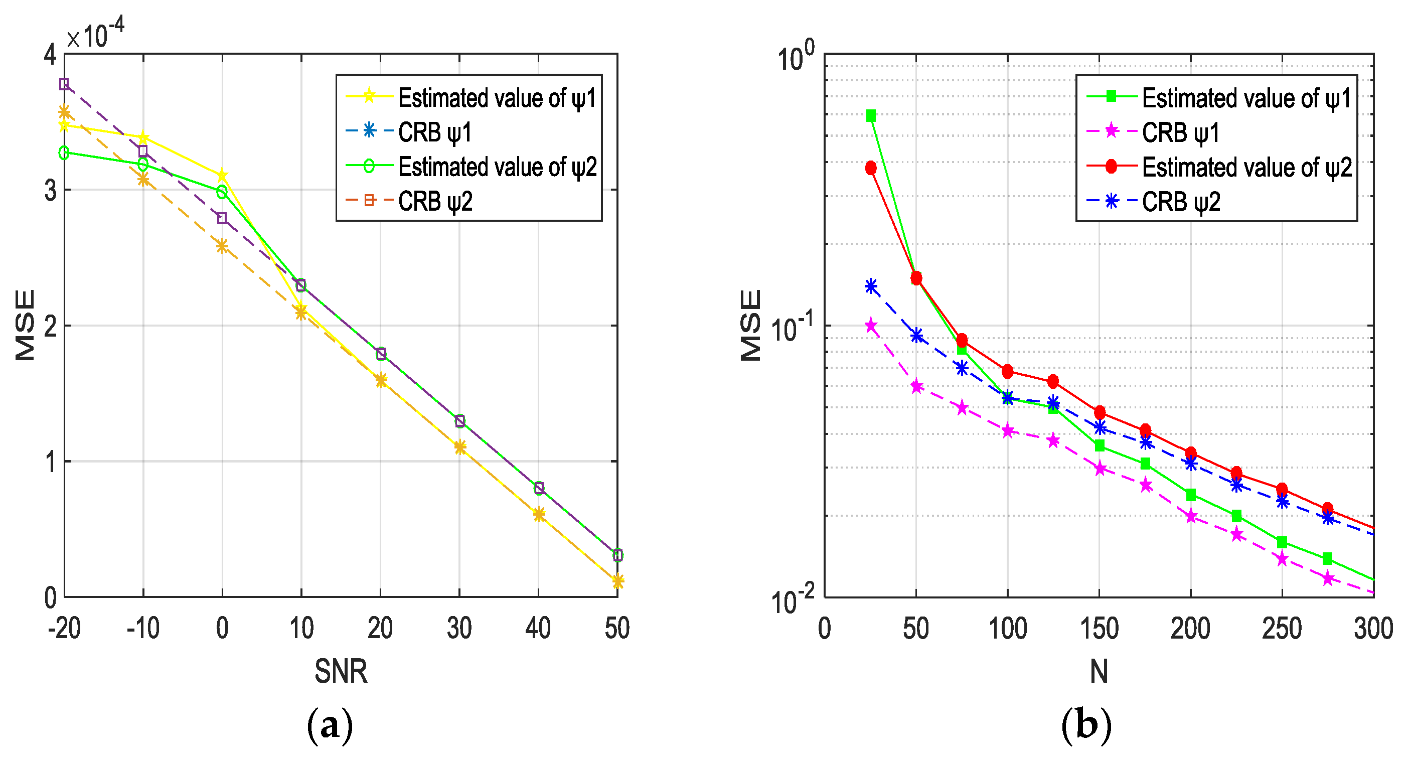
In the following noise simulation, the noise is Gaussian white noise with distribution feature (0, 0.0012), the SNR is in the range of −20~50 dB. Figure 9 shows the performance analysis of the amplitude offset estimation using the CML. It can be seen the MSE and the SNR of are smaller than those of . When SNR or N is large, it can be seen that the value of is constant. Combined with Table 1 and Table 2, when N is fixed, , the estimate can satisfy the SNR requirement, which is consistent with the condition of the maximum likelihood estimation.
As seen in Figure 9, when the SNR is fixed, the larger the number of samples, the smaller the MSE. When the number of samples is fixed, the larger the SNR, the smaller the value of MSE; the reason for this is that the higher the SNR, the better the channel condition. That is to say, the larger the SNR, the smaller the noise mixed in the signal, and the better the estimation of performance of the algorithm in this paper. Simulation results show that the anti-interference ability of the algorithm is better than the conventional DFT method. All the MSE values are only close to the CRB, but not lower than the lower limit of the cramerozone, which is consistent with theory that shows that CML has a good estimation performance for the phasor amplitude. Similar features are also reflected in phase angle estimation, as shown in Figure 10.
Figure 10 shows the performance analysis of the phase angle offset estimation using the CML. It can be found, except when N or SNR is very small, the MSE of is always smaller than that of , and when and , and have the same characteristics. In the case of low SNR, the SNR and the MSE of the estimated values of CML are not related. However, when the value of N is fixed, and , CML has the same characteristics as the angle deviation amplitude, the larger the number of samples, the more accurate the estimated value.
5.2. Steady State Test
5.2.1. Analysis of Harmonic and Noise Suppression
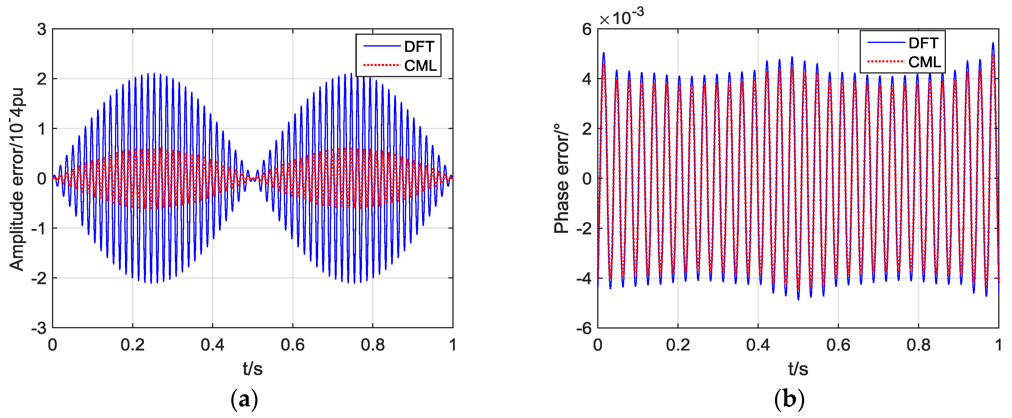
The harmonic signal is injected into the voltage and current signals:
b(t) is a Gaussian white noise with a distribution characteristic of N (0,0.0012), the signal is measured by the DFT method and the CML method respectively, the simulation results of phasor amplitude, phase angle and frequency error, and the total vector error (TVE) value are shown in Figure 11. TVE is the total vector error as follows [13]:
Xr(n) and Xi(n) are the real and imaginary parts of the true value of the phasor, and Xr and Xi are the real part and the imaginary part of the phasor estimation value.
It can be seen from Figure 11 that the CML and the DFT are greatly affected by the harmonics. The DFT cannot meet the maximum TVE error requirement in the standard. The CML of this paper has higher accuracy, which maintains the tracking speed, and increases the tracking accuracy of the signal.
5.2.2. Frequency Offset Simulation Analysis
The accuracy of the algorithm is simulated and analyzed when the frequency is offset, where the range of frequency offset is −3~3 Hz. The amplitude, phase angle error and TVE value of phasor measurement of DFT and CML are compared.
In Figure 12, the red line represents CML, the green line represents DFT. The measurement error of the two algorithms increases with the increase of frequency offset. However, the measurement error of CML is relatively small, and the error of DFT algorithm increases sharply with the increase of frequency. The amplitude, phase angle and TVE error of CML are far less than the DFT. Although with the increase of frequency offset, the measurement accuracy of the algorithm is reduced, it is still within the scope of the standard. The effect of signal frequency change on the measurement results is shown in Table 3.
As can be seen from Table 3, when the signal frequency is shifted by the nominal frequency, the measurement error of each parameter shows an increasing trend. When the frequency offset is very low, the accuracy of parameter measurement in this paper is still satisfied.
5.3. Dynamic Interference Test
In order to test the dynamic performance of the CML method, the dynamic simulation signal in the test is:
where, f = 50.5 Hz, sampling frequency fs = 1600 Hz, is the initial phase, the sampling points per cycle N = fs/f0 = 32. Taking into account the existence of changing factors in the power system, this section tests the dynamic performance of the algorithm by setting signal parameter mutations. In simulation, the frequency, amplitude and phase angle in Equation (37) are simultaneously mutated as follows: the frequency changes from 50 Hz to 50.5 Hz; the amplitude increases from 220 V Mutation to 200 V; the initial phase angle from 60° to 0° at t = 0.2425 s. Simulation results are shown in Figure 13.
As can be seen from Figure 13, when the system parameters are abrupt, both algorithms will produce short-term oscillations in the test, and will quickly resume their given state after oscillation. However, the traditional DFT algorithm has a significantly larger measurement error after the signal is abruptly changed. It can be seen that the CML method has the characteristics of fast convergence and accurate measurement results under the system dynamic conditions, and its dynamic characteristic have also been improved.
5.4. Application: Impedance Measurement Using CML Results under Noise Interference
When the system signal is a current signal, a similar estimation of the amplitude and phase of the current phasor can be made by using the CML method in this section. Using the phasor data measured by CML to estimate the impedance in the 10 kv distribution network, this result can be applied for fault location in the distribution network. The 10 kV distribution network is shown in Figure 14. When line l3 has a single-phase short-circuit fault through the transition resistance Rg at K. As the distribution network is seriously affected by harmonics, especially the odd harmonics, and the impedance under fault with added harmonics and noise is estimated as follows. The measurement signal is shown as Formula (35).
In Figure 14, inner impedance of source G1 ZG = (4.264 + j85.15) Ω, line impedance of line Z0 = (0.021 + j0.281) Ω/km, transformer impedance ZT = (0.05 + j12.1) Ω, transition resistance Rg = 2.5 Ω, the distance from the fault point K to the bus M P = 0.4l3, the length of the three lines l1 = 10 km, l2 = 15 km and l3 = 20 km respectively. The impedance estimated value obtained by the CML method is compared with the impedance measurement value and the impedance true value, and the error is shown in Figure 15 and Figure 16.
Since the system signal contains harmonic and noise, the actual impedance estimation is constantly changing over time. The change of the total resistance value of the distribution network model based on the CML method is shown in Figure 15. As can be seen from Figure 15, the actual value of the total resistance of the distribution network model is 7.507Ω, the estimated value of the resistance fluctuates constantly due to the noise, and the maximum deviation is about 0.072Ω. The accuracy of the resistance estimation based on the phasor values obtained by the CML method works better than conventional DFT method. Although the accuracy of the estimation is slightly lower than the measured value, it can simplify the measurement steps and improve the impedance measurement speed, which provides a new method for the fast and accurate fault location of the distribution network.
The change of the total reactance value of the distribution network model based on the CML method is shown in Figure 16. As can be seen from Figure 16, the estimated reactance is also changing over time. The maximum deviation between the estimated value and the actual value of 106.523 Ω is about 0.085 Ω. Since the reactance value is related to the system frequency, it is affected more by the system than the resistance, so its measurement deviation is greater than the resistance. The distribution network model has a large reactance base, so its relative error is very small. It can be seen that the estimation performance of reactance is ideal.
When a single-phase ground fault occurs at phase C at 0.20 s, the total impedance estimation values of the μPMU three channels at 0.245 s in Figure 14 are shown in Table 4. It can be seen from the deviation between the estimated impedance, and the real value in Table 4, that the impedance estimation accuracy based on CML estimates is satisfied. This method can be applied easily for fault location, state estimation and other advanced application in distribution networks.
6. Conclusions
In this paper, a new algorithm for simultaneous phasor estimation based on CML is proposed to solve the phasor parameters in the distribution network. When the parameter can be identified, its maximum likelihood estimated value can be determined by solving the vector orthogonal to the eigenvector of the parameter covariance matrix.
- (1)
- This algorithm uses the geometric edges and inner angles to solve the amplitude and phase, reducing the amount of computation. The performance of CML is verified by MSE, and the signals under harmonic, noise and frequency offset are tested. The results meet the requirements of IEEE C37.118, and the algorithm has less calculation burden for μPMU, compared with DFT.
- (2)
- The dynamic test of the CML method is carried out and the impedance of the distribution network model is solved according to the phasor estimation results of CML method. The simulation shows that the impedance estimation performance based on the CML measurement value is satisfied.
- (3)
- The phasor measurement algorithm proposed in this paper can be applied to fault location, state estimation, and other advanced application in distribution networks, because of numerical stability and estimation precision under a quasi-steady-state condition.
The proposed CML method can improve estimation precision of phasor and balance three-phase effect. The future research work will focus on the advanced application of μPMU for distribution networks.
Author Contributions
J.L. and W.W. conceived and designed the simulation; J.L. and W.W. analyzed the data; and J.L., S.Z., C.G. wrote the paper. All the authors read and confirmed the final manuscript.
Conflicts of Interest
The authors declare no conflict of interest.
References
- Hamelink, J.B.; Nguyen, P.H.; Kling, W.L.; Ribeiro, P.F.; De Groot, R.J. Routing power flows in distribution networks using locally controlled power electronics. In Proceedings of the Universities Power Engineering Conference, London, UK, 4–7 September 2012; pp. 1–6. [Google Scholar]
- Fei, C.; Dong, L.; Chen, Y.; Center, D. Hierarchically distributed voltage control strategy for active distribution network. Autom. Electr. Power Syst. 2015, 39, 61–67. [Google Scholar]
- Phadke, A.G.; Thorp, J.S. Synchronized Phasor Measurements and Their Applications; Springer: New York, NY, USA, 2008; pp. 93–169. [Google Scholar]
- Bollen, M.H.J.; Gu, I.Y.H.; Santoso, S.; McGranaghan, M.F.; Crossley, P.A.; Ribeiro, M.V.; Ribeiro, P.F. Bridging the gap between signal and power. IEEE Signal Process. Mag. 2009, 26, 12–31. [Google Scholar] [CrossRef]
- Borges, F.A.S.; Fernandes, R.A.S.; Silva, I.N.; Silva, C.B.S. Feature extraction and power quality disturbances classification using smart meters signals. IEEE Trans. Ind. Inform. 2017, 12, 824–833. [Google Scholar] [CrossRef]
- Su, P.; Wang, H. Discussion of the short-window Morlet complex wavelet algorithm on the power system signal process. Autom. Electr. Power Syst. 2004, 28, 36–42. [Google Scholar]
- Mahmood, F.; Hooshyar, H.; Lavenius, J.; Lund, P.; Vanfretti, L. Real-time reduced steady state model synthesis of active distribution networks using PMU measurements. IEEE Trans. Power Deliv. 2017, 32, 546–555. [Google Scholar] [CrossRef]
- Su, H.Y.; Liu, T.Y. A PMU-Based method for smart transmission grid voltage security visualization and monitoring. Energies 2017, 10, 1103. [Google Scholar]
- Roberts, C.M.; Shand, C.M.; Brady, K.W.; Stewart, E.M.; Mcmorran, A.W.; Taylor, G.A. Improving distribution network model accuracy using impedance estimation from micro-synchrophasor data. In Proceedings of the IEEE Power & Energy Society General Meeting, Boston, MA, USA, 17–21 July 2016; pp. 1–5. [Google Scholar]
- Jia, K.; Gu, C.; Li, L.; Xuan, Z.; Bi, T.; Thomas, D. Sparse voltage amplitude measurement based fault location in large-scale photovoltaic power plants. Appl. Energy 2018, 211, 568–581. [Google Scholar] [CrossRef]
- Wang, D.; Wilson, D.; Venkata, S.; Murphy, G. PMU-based angle constraint active management on 33kV distribution network. In Proceedings of the International Conference and Exhibition on Electricity Distribution, Stockholm, Sweden, 10–13 June 2013; pp. 1–4. [Google Scholar]
- Mai, R.; He, Z.; Brian, K.; Bo, Z. A maximum likelihood based dynamic synchrophasor estimator for online purpose. In Proceedings of the IEEE Power & Energy Society General Meeting, Calgary, AB, Canada, 26–30 July 2009; pp. 1–5. [Google Scholar]
- IEEE Standards. C37.118.1-2011-IEEE Standard for Synchrophasor Measurements for Power Systems; Revision of IEEE Std C37.118-2005; IEEE: Piscataway, NJ, USA, 2011; pp. 1–61. [Google Scholar]
- Wu, K.; Zheng, S.; An, S.; Ding, X.; Zhang, F. A dynamic display method of distribution network’s monitoring information. In Proceedings of the IEEE International Conference on Software Engineering and Service Science, Beijing, China, 23–25 September 2015; pp. 710–713. [Google Scholar]
- Stoica, P.; Nehorai, A. Music, maximum likelihood, and Cramer-Rao bound. IEEE Trans. Signal Process. 2007, 37, 720–741. [Google Scholar] [CrossRef]
- Bollen, M.; Gu, I. Signal Processing of Power Quality Disturbances; John Wiley & Sons Inc.: Hoboken, NJ, USA, 2006. [Google Scholar]
- Horn, R.A.; Johnson, C.R. Matrix Analysis; Cambridge University Press: Cambridge, UK, 2012. [Google Scholar]
- Renaux, A.; Forster, P.; Chaumette, E.; Larzabal, P. On the High-SNR conditional maximum-likelihood estimator full statistical characterization. IEEE Trans. Signal Process. 2006, 54, 4840–4843. [Google Scholar] [CrossRef]
- Nguyen, C.T.; Srinivasan, K. A new technique for rapid tracking of frequency deviations based on level crossings. IEEE Trans. Power Appar. Syst. 1984, 103, 2230–2236. [Google Scholar] [CrossRef]
- Kun, Z.; Lei, Y.; Li, L.; Li, Q.; Lang, Y.S.; Jia, P.Y. A method of introducing PMU current measurement to nonlinear state estimation. Adv. Mater. Res. 2014, 10, 2816–2821. [Google Scholar] [CrossRef]
- Ren, Y. Low-voltage power distribution system fault protection and protection of electrical equipment selection. Build. Electr. 2016, 7, 3–10. [Google Scholar]
- Sengijpta, S. Fundamentals of statistical signal processing: Estimation theory. Technometrics 1998, 37, 465–466. [Google Scholar] [CrossRef]
Figure 1.
Three-phase three wire system.

Figure 2.
Geometric interpretation of Formula (22).

Figure 3.
Geometric interpretation of the three-phase symmetrical system.

Figure 4.
Diagram of one branch.

Figure 5.
Three-phase four wire wiring diagram.

Figure 6.
Geometric interpretation of Formula (27).

Figure 7.
Flowchart of the proposed algorithm in μPMU.

Figure 8.
The sinusoidal amplitude and phase modulation.

Figure 9.
Estimation of amplitude parameter and . (a) Noise and mean square error (MSE); and (b) The variation of mean square error (MSE) with signal to noise ratio (SNR).
Figure 9.
Estimation of amplitude parameter and . (a) Noise and mean square error (MSE); and (b) The variation of mean square error (MSE) with signal to noise ratio (SNR).

Figure 10.
Estimation of phase parameter and . (a) The variation of mean square error (MSE) with signal to noise ratio (SNR); and (b) Noise and mean square error (MSE).
Figure 10.
Estimation of phase parameter and . (a) The variation of mean square error (MSE) with signal to noise ratio (SNR); and (b) Noise and mean square error (MSE).

Figure 11.
Simulation of amplitude, phase angle, frequency and TVE error of CML under harmonic and noise interference. (a) The amplitude error of CML varying with time; and (b) Phase angle error and time; and (c) Frequency error and time; and (d) The total vector error and time.
Figure 11.
Simulation of amplitude, phase angle, frequency and TVE error of CML under harmonic and noise interference. (a) The amplitude error of CML varying with time; and (b) Phase angle error and time; and (c) Frequency error and time; and (d) The total vector error and time.


Figure 12.
Amplitude, phase and TVE error of CML in frequency offset.(a) The relation between amplitude error and frequency offset and time variation; and (b) The relation between Phase error and frequency offset and time variation; and (c) The relation between the total vector error and frequency offset and time variation.

Figure 13.
Phasor amplitude, phase angle and TVE error in the parametric abrupt change test. (a) The relationship between amplitude error and time; and (b) Phase angle error and time; and (c) the total vector error and time.
Figure 13.
Phasor amplitude, phase angle and TVE error in the parametric abrupt change test. (a) The relationship between amplitude error and time; and (b) Phase angle error and time; and (c) the total vector error and time.

Figure 14.
10 kv distribution system model.

Figure 15.
Total resistance measurement error of the distribution network model.

Figure 16.
Total reactance measurement error of the distribution network model.


Table 1.
The relationship between CRB, var and bias2 of dk when .
| Experimental Value | Estimated Value | |||||||
|---|---|---|---|---|---|---|---|---|
| N | CRB | MSE | Var() | Bias2(dk) | MSE | Var() | Bias2(dk) | |
| 100 | 0.0178 | 0.0181 | 0.0181 | 0.0013 | 0.0193 | 0.0192 | 0.0013 | |
| 200 | 0.0101 | 0.0113 | 0.0113 | 0.0007 | 0.0127 | 0.0127 | 0.0008 | |
| 1000 | 0.0026 | 0.0028 | 0.0028 | 0.0001 | 0.0031 | 0.0031 | 0.0000 | |
| 100 | 0.0495 | 0.0513 | 0.0513 | 0.0010 | 0.0524 | 0.0524 | 0.0011 | |
| 200 | 0.0281 | 0.0297 | 0.0297 | 0.0004 | 0.0309 | 0.0308 | 0.0003 | |
| 1000 | 0.0069 | 0.0071 | 0.0071 | 0.0001 | 0.0073 | 0.0073 | 0.0000 | |
Table 2.
The relationship between CRB, var and bias2 of dk when N = 200.
| Experimental Value | Estimated Value | |||||||
|---|---|---|---|---|---|---|---|---|
| SNR dB | CRB | MSE | Var () | Bias2(dk) | MSE | Var() | Bias2(dk) | |
| 5 | 0.00023 | 0.00023 | 0.00023 | 0.00011 | 0.00024 | 0.00024 | 0.00012 | |
| 15 | 0.00017 | 0.00017 | 0.00017 | 0.00008 | 0.00018 | 0.00018 | 0.00008 | |
| 25 | 0.00014 | 0.00014 | 0.00014 | 0.00005 | 0.00016 | 0.00016 | 0.00006 | |
| 5 | 0.00016 | 0.00013 | 0.00012 | 0.00007 | 0.00014 | 0.00018 | 0.0008 | |
| 15 | 0.00012 | 0.00012 | 0.00012 | 0.00004 | 0.00013 | 0.00013 | 0.00004 | |
| 25 | 0.00008 | 0.00008 | 0.00008 | 0.00001 | 0.00007 | 0.00008 | 0.00001 | |
Table 3.
The influence of the signal frequency changes on the measurement results.
| f/Hz | The Maximum Amplitude Error (%) | The Maximum Phase Angle Error (°) | The Maximum TVE Error (%) |
|---|---|---|---|
| 49.7 | 0.095 | 0.029 | 2.017 |
| 49.8 | 0.068 | 0.018 | 1.003 |
| 49.9 | 0.037 | 0.011 | 0.008 |
| 50.0 | 3.488 × 10⁻⁹ | 1.013 × 10⁻⁸ | 3.491 × 10⁻⁹ |
| 50.1 | 0.037 | 0.030 | 0.008 |
| 50.2 | 0.069 | 0.019 | 1.001 |
| 50.3 | 0.096 | 0.013 | 2.019 |
Table 4.
The actual and estimated values of distribution network impedance at 0.245 s.
| Actual Value (Ω) | Measured Value (Ω) | Estimated Value (Ω) | Deviation (Ω) | |
|---|---|---|---|---|
| Load 1 | 4.524 + j100.060 | 4.519 + j100.065 | 4.455 + j99.980 | 0.069 + j0.080 |
| Load 2 | 4.629 + j101.465 | 4.622 + j101.469 | 4.558 + j101.546 | 0.070 + j0.081 |
| Load 3 | 6.982 + j99.498 | 6.978 + j99.453 | 6.909 + j99.577 | 0.073 + j0.079 |
| Total load | 7.507 + j106.523 | 7.502 + j106.529 | 7.436 + j106.605 | 0.071 + j0.082 |
© 2018 by the authors. Licensee MDPI, Basel, Switzerland. This article is an open access article distributed under the terms and conditions of the Creative Commons Attribution (CC BY) license (http://creativecommons.org/licenses/by/4.0/).
Share and Cite
MDPI and ACS Style
Li, J.; Wei, W.; Zhang, S.; Li, G.; Gu, C. Conditional Maximum Likelihood of Three-Phase Phasor Estimation for μPMU in Active Distribution Networks. Energies 2018, 11, 1320. https://doi.org/10.3390/en11051320
AMA Style
Li J, Wei W, Zhang S, Li G, Gu C. Conditional Maximum Likelihood of Three-Phase Phasor Estimation for μPMU in Active Distribution Networks. Energies. 2018; 11(5):1320. https://doi.org/10.3390/en11051320
Chicago/Turabian StyleLi, Jiang, Wenzhen Wei, Shuo Zhang, Guoqing Li, and Chenghong Gu. 2018. "Conditional Maximum Likelihood of Three-Phase Phasor Estimation for μPMU in Active Distribution Networks" Energies 11, no. 5: 1320. https://doi.org/10.3390/en11051320
Note that from the first issue of 2016, this journal uses article numbers instead of page numbers. See further details here.