Hybrid Coupled Multifracture and Multicontinuum Models for Shale Gas Simulation by Use of Semi-Analytical Approach

1
School of Computer & Information Technology, Northeast Petroleum University, Daqing 163318, China
2
Research Institute of Petroleum Exploration & Development, PetroChina, Beijing 100083, China
3
PetroChina Southwest Oil & Gasfield Company, Chengdu 610500, China
4
Computer Science School, Southwest Petroleum University, Chengdu 610500, China
5
Sinopec Zhongyuan Gas Corp. Ltd., Sinopec Corp, Puyang 457000, China
*
Author to whom correspondence should be addressed.
Energies 2018, 11(5), 1308; https://doi.org/10.3390/en11051308
Submission received: 26 April 2018
/
Revised: 5 May 2018
/
Accepted: 14 May 2018
/
Published: 21 May 2018
(This article belongs to the Section L: Energy Sources)
Abstract
:Combining the advantages of multicontinuum and multifracture representations provides an easy-to-use tool to adequately capture the characteristic of the multiscaled fracture system in shale gas reservoir. A hybrid model is established on the basis of simplified conceptual productivity assumption, where the matrix volume is divided into two sub-domains (triple-porosity model and dual-depletion flowing model) and the fracture volume is represented by discrete finite conductivity fracture. In addition, the mechanisms of instant desorption, viscous flow and dual-depletion in matrix are taken into account. The rate transient responses are then obtained by use of semi-analytical approach. Based on the model, type curves are plotted and verified by comparing with alternative reliable methods. Different flow regimes in shale gas reservoirs can be identified and detected. The Generalized Likelihood Uncertainty Estimation methodology, based on probabilistic aggregation theory, is employed to integrating those two productivity models together such that the production can be predicted more accurately. A field example is applied to validate the applicability of this new model. Finally, it is concluded that the proposed model can predict the rate and cumulative rate more easily and practically.
1. Introduction
Shale gas reservoir is typical unconventional reservoir due to its ultra-low permeability and porosity. Generally speaking, there is no natural productive capacity for such reservoirs. Multi-stage fracturing technology for horizontal wells can activate the pre-existing natural fractures and generate a complex fracture network called stimulated reservoir volume (SRV), which has become the most effective method to develop shale resources [1]. Generally, SRV is defined as the part of the drainage area impacted by hydraulic fractures and concomitant reactive fractures, where the productivity of shale gas well could be effectively improved [2,3,4,5,6].
To characterize the transient performance for shale gas reservoirs, many scholars have made some efforts to simulate the fluids flow and transport behaviors in such complexly-structured fracture network through analytical and semi-analytical solutions [7,8,9,10]. These solutions are mostly proposed in the terms of multi-porosity model and multi-linear model. For the multi-porosity model, Barenblatt [11] and Warren and Root [12] firstly proposed the dual-porosity model to simulate the fluid exchange between matrix and fractures, where the exchange is assumed in the pseudo steady state. Then, alternative transient models were proposed for simulating the fluid transfer between matrix and fractures [13,14,15], which relaxed the pseudo-steady assumption. In addition, various triple-porosity models were subsequently established to overcome the drawback of the dual-porosity model in terms of multi-scale porosity description, such as dual-fracture/triple-porosity models [16] and improved triple-porosity/permeability model [17,18,19]. Next, for multi-linear model, numerous field practices demonstrate that many fractured reservoirs exhibit linear flow, which could last for several years. El-Banbi [20] proposed a linear dual-porosity model for linear fractured reservoirs without considering the impact of desorption, diffusion. Hasan and Al-Ahmadi [21] proposed a triple-porosity linear flow model with consideration of the impact of shale gas desorption and diffusion. Zhao et al [22] proposed a triple-porosity spherical flow model for the fractured infinite shale gas reservoirs by considering the impact of diffusion and desorption. Obinna and Hassan [23] proposed the quadrilinear flow mode to simultaneously the depletion from the matrix into natural and hydraulic fractures.
Nevertheless, it is very difficult to use these multi-porosity/linear models mentioned above to investigate the actual performance for shale gas reservoirs. It is caused by the fact that the characterization of diffusion and adsorption is not taken into account. Therefore, it is necessary to comprehensively take the impact of various flowing mechanisms and multi-porosity characteristics into account to obtain critical dynamic parameters for shale gas reservoirs. In this paper, for the purpose of obtaining accurate results of performance analysis, the main work is twofold: proposing two improved models to simulate production performance, and presenting a reliable probabilistic algorithm to integrate these two models. It is noted that the fundamental model is established on the basis of the work presented by Obinna and Hassan [23]. Some improvements are made: (1) SRV zone is simulated as a triple-porosity cubic model by taking into account instant adsorption and viscous flow; (2) two kinds of simplified conceptual models are generated to divide the matrix volume into two sub-domains for the purpose of allowing simultaneous matrix-hydraulic fracture (HF) and matrix-natural fracture (NF) depletion. Subsequently, the Generalized Likelihood Uncertainty Estimation (GLUE) approach is built, based on probabilistic aggregation theory, in order to reduce the uncertainty of performance analysis by integrating those two models. Finally, the numerical simulation and field application are applied to validate this new simplified aggregation model. The improved method in this paper could provide a robust methodology approach to quantify the uncertainty of production prediction.
2. Productivity Model
A schematic for the improved model is presented in Figure 1. Figure 1a shows the model consists of SRV region, unstimulated reservoir volume (USRV) region, and fracture region. Figure 1b shows the simultaneous matrix-depletion into HF and NF. In addition, some assumptions are emphasized as follows:
- SRV region is simplified as a cubic triple-porosity model, containing natural fractures, hydraulic fractures and the matrix;
- Hydraulic fractures are perpendicular to the horizontal well and evenly distributed along the wellbore, and the natural fractures are perpendicular to the hydraulic fracture. Horizontal wellbore are equal to L, and the length of hydraulic fracture and the width of reservoir are equal to ye;
- Hydraulic fracture is finite conductivity and assumed to be penetrated fully;
- Only the fluid flowing from hydraulic fractures to wellbore is considered;
- Simultaneous matrix-depletion into HF and NF is assumed pseudo-steady state, and the exchange between HF and NF is assumed unsteady state;
- The effect of gravity and capillary pressure is not taken into account;
- Gas is slightly compressible and the compressibility coefficient is constant;
- This paper considers the simultaneous depletion from the matrix into HF and NF. The matrix in SRV region is artificially divided into two distinct segments which are denoted as sub-matrix m1 and sub-matrix m2 respectively. The depletion process from the matrix to HF and NF in SRV region (seen in Figure 1b);
- Sub-matrix m1 feeds the HF via inter-porosity exchange;
- Sub-matrix m2 feeds the NF via inter-porosity exchange.
The conceptual model can get some further detailed divisions based on different methods. Hence, two different approaches would be developed to characterize dual-depletion in the following section.
2.1. Conceptual Model
2.1.1. Conceptual Model 1
The matrix is divided into two sections. Some further assumptions are made to derive the following formulas:
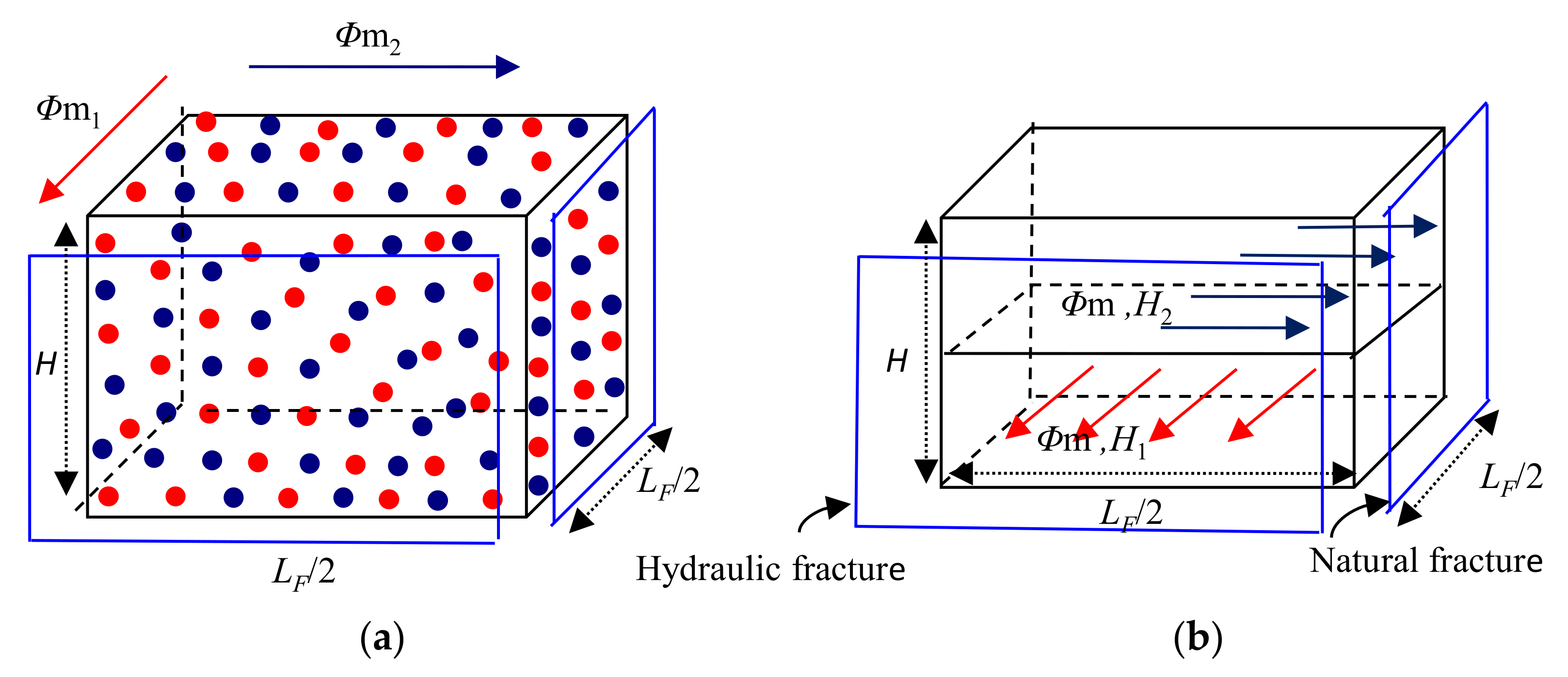
- Sub-matrix m1 and sub-matrix m2 mix up with each other evenly, which means that both of them have the same width Lf, length LF and thickness H (see the Figure 2a);
- Sub-matrix m1 and sub-matrix m2 have different porosities denoted as Φm1 and Φm2, and the total porosity of the total matrix denoted as Φm is the sum, presented as:
Based on the assumptions mentioned above, the pore volume ratio χ is introduced to describe this characterization [24], which satisfies:
2.1.2. Conceptual Model 2
The matrix is artificially divided into two sections. Some further assumptions are made to derive the following formulas:
- Sub-matrix m1 and sub-matrix m2 are strictly separated in the vertical direction, and the whole matrix is divided into two layers.
- Sub-matrix m1 and sub-matrix m2 have different thicknesses denoted as H1 and H2, and the total thickness of the matrix is denoted as H, which is the sum of those two parts:
Based on the assumptions, the thickness ratio γ is introduced to describe this character, and the definition of this parameter is derived as:
2.2. Mathematical Model
Based on the mass balance principle, the governing equations considering the adsorption, desorption and viscous flowing can be established respectively (see Appendix A).To simplify these equations, dimensionless variables are introduced (see in Table 1), and then the final dimensionless governing equations are derived.
2.2.1. Conceptual Model 1
For Model 1, the corresponding equation governing fluid flowing is presented as follows:
- The pressure equation governing fluid flow in hydraulic fracture is given as:
- The pressure equation governing fluid flow in natural fracture is given as:
- The pressure equation governing fluid flow in matrix 1 is given as:
- The pressure equation governing fluid flow in matrix 2 is given as:
2.2.2. Conceptual Model 2
In the upper layer unit, the mathematical model is described by the following differential equations.
- The pressure equation governing fluid flow in hydraulic fracture is given as:
- The pressure equation governing fluid flow in natural fracture is given as:
- The pressure equation governing fluid flow in matrix 2 is given as:In the lower layer unit, the mathematical model is described by the following differential equations.
- The pressure equation governing fluid flow in hydraulic fracture is given as:
- The pressure equation governing fluid flow in natural fracture is given as:
- The pressure equation governing fluid flow in matrix 1 is given as:
In addition, the corresponding conditions are list in Table 2.
2.3. Model Solution
The Laplace transformation is used to solve Equations (6)–(15), the details of derivation are presented in Appendix B. As shown from Equations (A37) and (A41), the final solutions of these equations in Laplace space are derived as:
For Model 1, the dimensionless production rate is given as
For Model 2, the dimensionless production rate is given as
However, to analyze the impact of relative parameters and identify flow regimes, the rate transient responses must be inverted into real time space by using the Stehfest numerical inversion algorithm [25].
3. Results and Discussion
In this model, some characterized parameters includes: ωF, ωf, ωm, χ, γ.
3.1. Model Validation
3.1.1. Validation with Analytical Approach
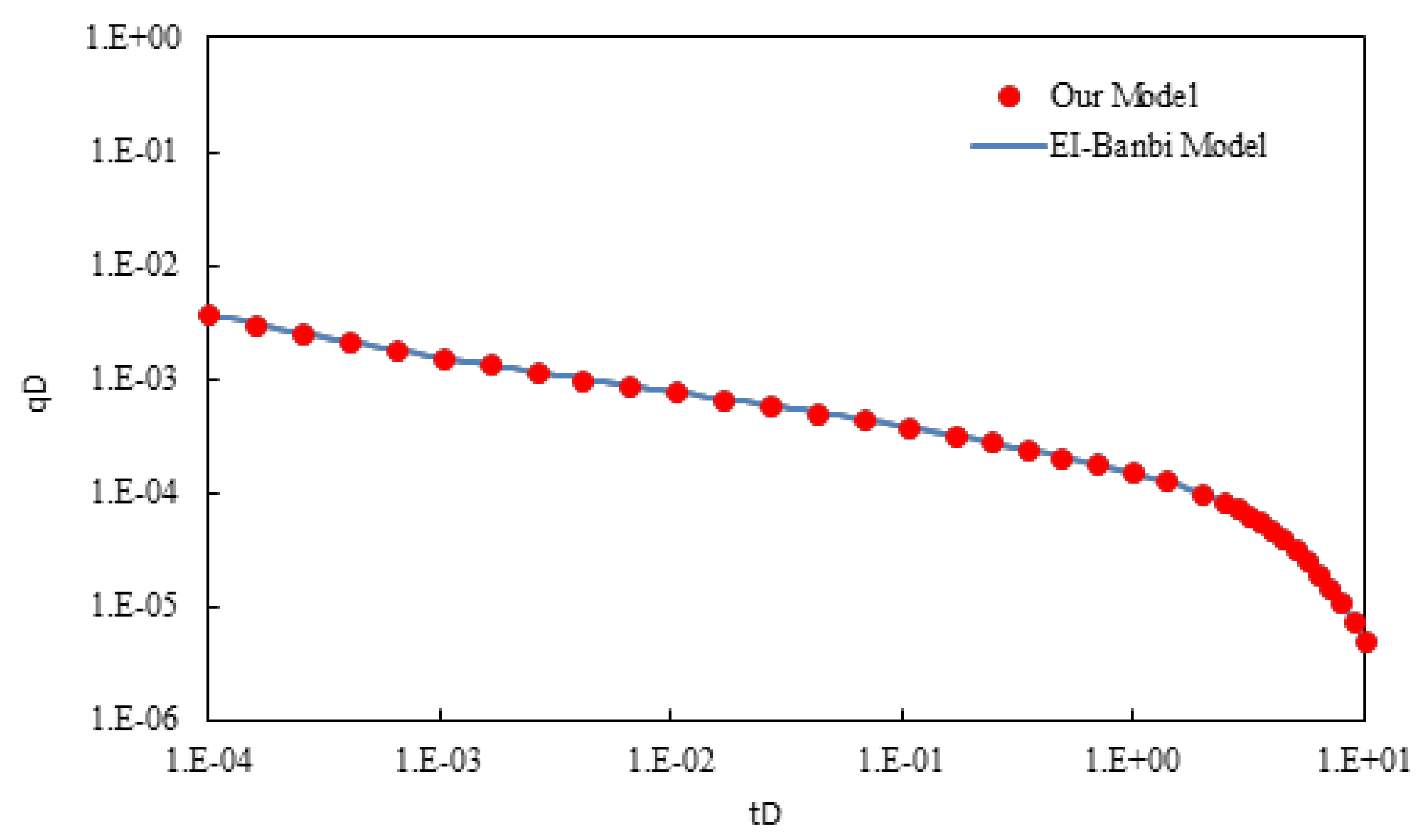
When these parameters are equal to a special value, the new model proposed in this paper can be varied to alternative models which have been verified reasonable. For example, when ωf is equates to 0, the model can be simplified as dual porosity slab model [26]; when χ = 0 or γ = 0, it indicates that the gas only depletes from matrix to NF [21]. Put another way, the new model can be equivalent to the traditional triple-linear model [20]. In summary, this new model can be universally applied to different formations only if some characterized parameters are equal to the corresponding values. Figure 3 displays the comparison of our model with alternative approach in the case of linear flow. Our model has a significant agreement with El-Banbi model [20] during the whole production cycle.
3.1.2. Validation with Numerical Approach
Furthermore, a numerical simulation is conducted to compare with the models (the input data are listed in Table 3). The commercial software Eclipse 2010 (Eclipse Foundation, Ottawa, ON, Canada) is selected to simulate the behavior of triple-porosity reservoirs and verify the semi-analytical solutions in this paper.
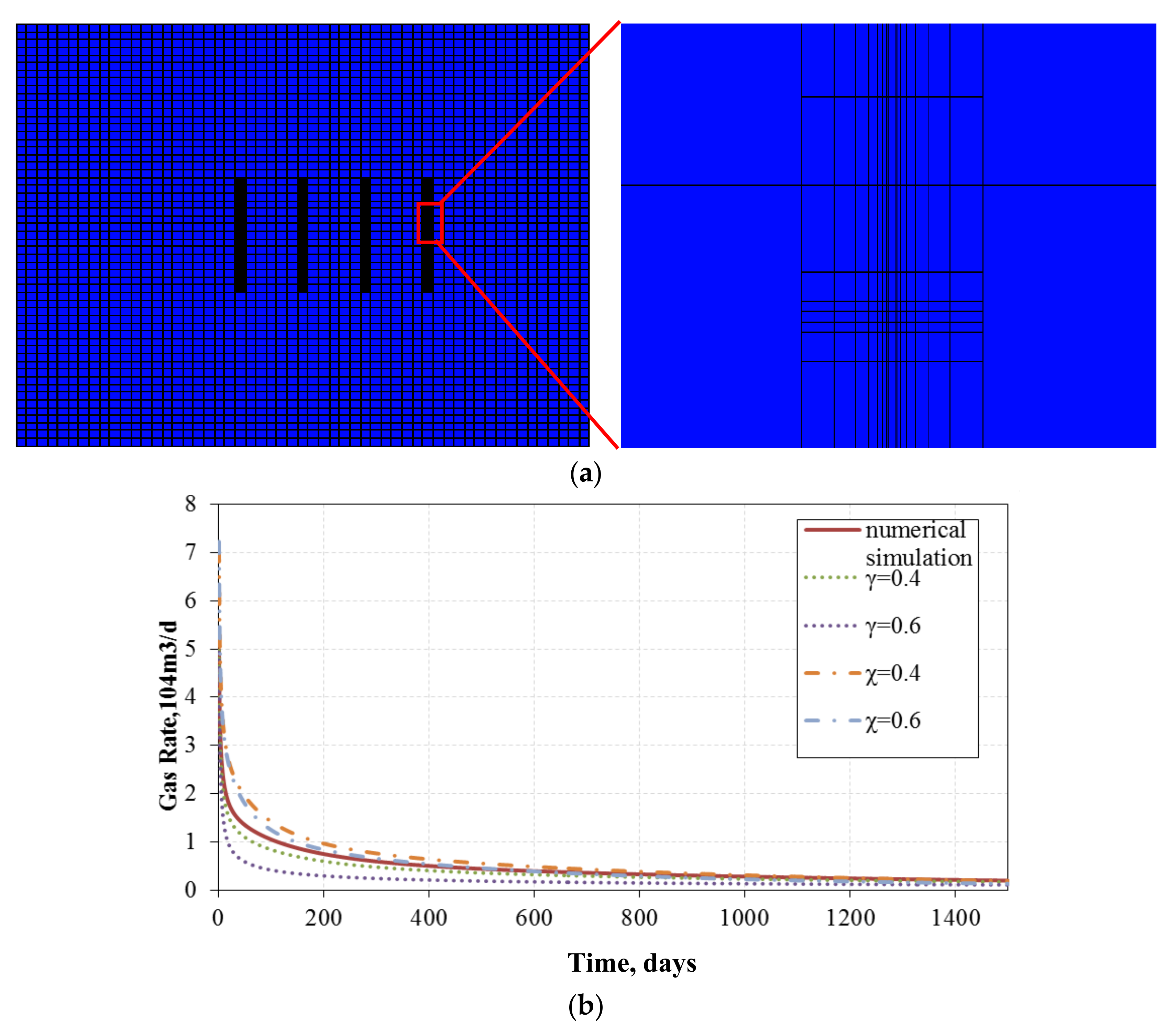
The numerical model considers the flow influx towards the horizontal wellbore. Considering the symmetrical structure of the multi-fractured horizontal well, one representative segment is selected to represent one quadrant of the reservoir volume around a hydraulic fracture. This segment contains twenty micro fractures orthogonal to the hydraulic fractures at 10 m fracture spacing. As shown in Figure 4a, the model is built to be a two dimension model with 100 grid cells in the x-direction, 100 grid cells in y-direction and only one grid cell in the z-direction. The multi-porosity method is applied to further divide the matrix, thus the transient flow in the matrix can be simulated. Additionally, the desorption model is instant. The local grid refinement (LGR) method is employed to create the hydraulic fractures. Only then is the multi-stage hydraulic fracturing simulated. From the comparison results of transient rate in Figure 4b, the semi-analytical results in this paper are consistent with the results from numerical model.
Based on the model verification, it is proved that our model is accurate and can be further used to calculate more complex case.
3.2. Sensitivity Analysis
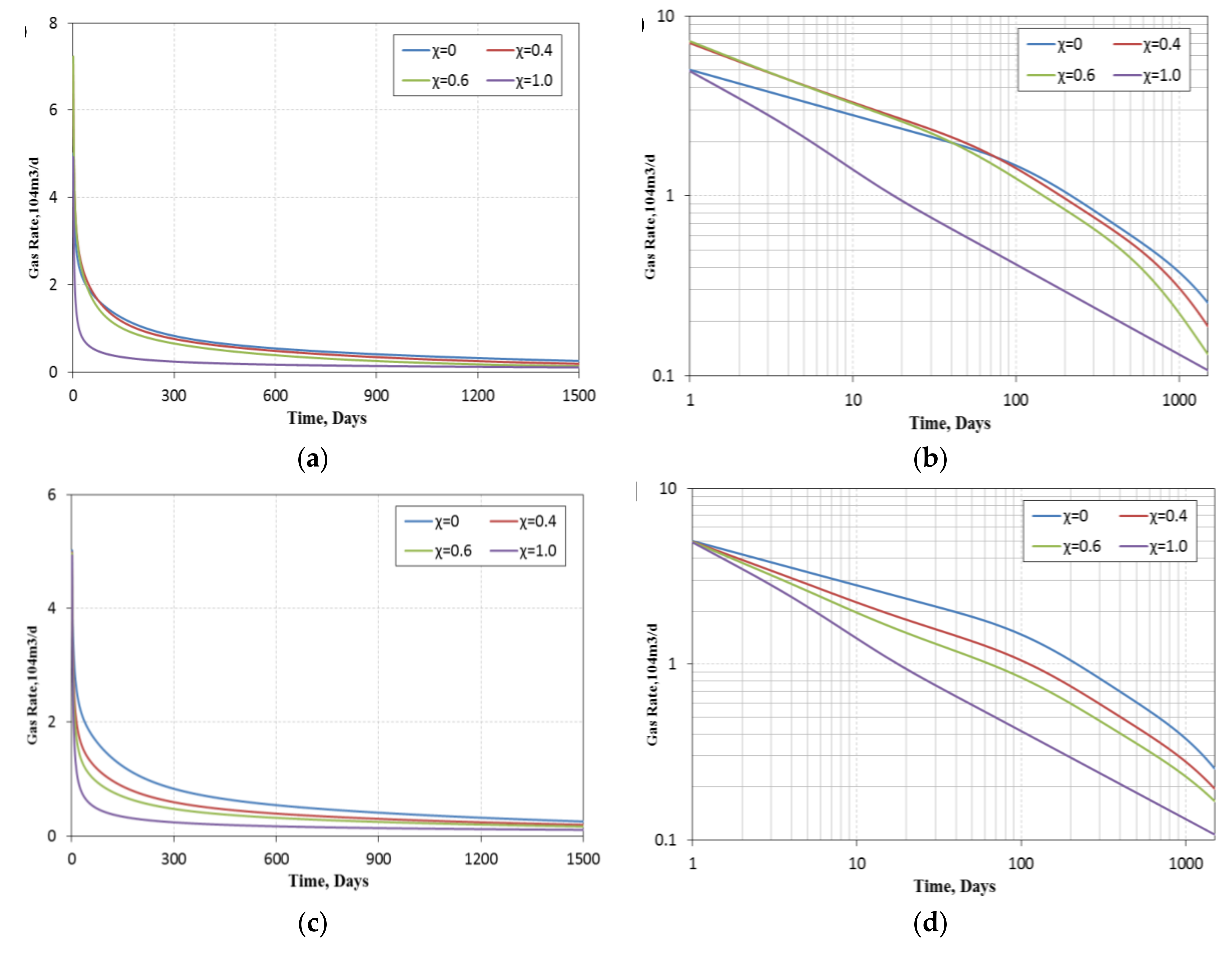
In this subsection, the parameters used are put into Table 3. The transient rate behavior is achieved by using Stehfest algorithm [25]. Figure 5 demonstrates the type curves of transient rate behavior for new model, where these curves are respectively shown in log-log and regular plots.
Seen from the type curve in Figure 5b,d, some well-known flowing regimes can be identified, such as the bilinear flow (the slope of curve is identify by −0.25), the linear flow (the slope of curve is identified by −0.5) and the boundary dominated flow (the slope of curve is approximately identified by −0.25).
Due to the limitation of χ and γ, it is possible that some flow regimes could not be identified. Under the assumption that (1) χ = 0 and γ = 0 or (2) χ = 1 and γ = 1, the two models are equivalent, which indicates that the characterization of flow regimes caused by two models is identical.
For model 1 seen in Figure 5a,b, with the increase of the pore volume ratio χ, the gas rate firstly increases and then decreases. When matrix and NF simultaneously deplete into HF, desorption occurs earlier and the rate is higher. However, when gas depletes from the matrix to HF, the boundary dominated flow occurs earlier, so the gas rate become lower. In term of model 2 seen in Figure 5c,d, with the increase of the thickness ratio γ, gas rate decreases. Model 2 assumes that there is no connection between the upper and lower layers. Meanwhile, the matrix and NF have no connection in the lower layer, so the impact of boundary is more severe and the gas rate decreases.
It is noted that this phenomenon mentioned above is not the most interesting part in this paper. By comparing Figure 5a,c, it is easily found that the gas rate is distinct at the early production period (less than 2 years), dependent on the pore volume ratio χ and the thickness ratio γ. During late production period, the gas rate is approximately identical under different values of χ and γ. It is a significant discovery in the field of reservoir engineering when conducting production prediction and estimating recovery in the case that the available data are limited, especially for shale gas wells. If pore volume ratio χ or thickness ratio γ are presented in the reasonable range, model 1 or 2 can perfectly match with the actual production data at the early stage, and then the future performance of gas well can be predicted based on the matched model. It is the reason that the intermediate- and late-time production performance is almost independent on the values of pore volume ratio χ or thickness ratio γ.
4. Model Aggregation
The numerical and semi-analytical results have been presented in Figure 4b. It is emphasized that the semi-analytical transient rate behavior presented by model 1 is higher than model 2. However, the rate predicted from the numerical simulation is in the range of two models. It indicates that the simulated curve of model 1 overlies model 2 during the whole production period when the value of pore volume ratio χ or thickness ratio γ is reasonable. Therefore, it makes sense to integrate the two models together to develop a generalized framework model for eliminating the error when predicting future performance of gas well. Here, an approach of Generalized Likelihood Uncertainty Estimation (GLUE) methodology is employed [27]. The approach of GLUE is presented based on the probabilistic aggregation theory. Using this approach, these two models can be integrated according to the personal weight which reduces the uncertainties.
4.1. GLUE Method
The theory of the GLUE method will be discussed in this section. When the pore volume ratio χ and thickness ratio γ can be reasonably chosen, the resulting simulation based on new model could provide better matching of limited history data. However, there exists remarkable error on rate prediction.
This study proposed an approach to integrate these two models, which includes two steps. (1) Two models are used to match the data to obtain reasonable values of the pore volume ratio χ and the thickness ratio γ; (2) A weight is assigned to each model based on some goodness-of-fit statistics, and then weighted mean and standard deviation of desired performance measures (the rate and cumulative rate) could be calculated. Here, a simple likelihood measure in the GLUE method can be defined using the root-mean-square-error (RMSE):
where, RMSEj represents the j-th model, j = 1, 2 in this paper. Normalizing the likelihoods, the sum is equal to one, which provides the GLUE weight for the two models:
where, Lj is the likelihood functions, PRj is the prior weight of each model (i.e., PRj = 1/2 if all are assumed to be equally likely prior weighting). From these weights, the integrated gas rate q and cumulative rate G on certain production time T0 can be calculated as:
and the standard deviation can be computed from:
4.2. Application Illustration
4.2.1. Procedure
Based on above analysis, the procedure would be divided into three steps:
- Actual production data are matched based on model 1 and model 2 respectively. As a result, the most reliable value of pore volume ratio χ and thickness ratio γ can be obtained;
- Based on history and predicted curves, the likelihoods can be calculated respectively for model 1 and model 2 using Equation (18), and then the likelihoods can be normalized using Equation (19);
- Based on Equation (20), we can calculate the production rate and cumulative rate at a certain production time T0, and then compare those results with the numerical simulation by calculating standard deviation using Equation (21).
4.2.2. Field Example
A multi-stage fractured horizontal well is chosen from certain shale gas zone in Sichuan Basin, China. The geometry and distribution of hydraulic fractures can be diagnosed with seismic events during hydraulic-fracturing treatment. Fracture locations are interpreted by using the event amplitude as an intensity measure, and fracture sizes are estimated by the relationship between the amplitude and the seismic moment. It can be seen from Figure 6, the direction of fracture is N570E for this well. The basic data from the well testing and the core analysis are listed in Table 4.
In Figure 7, the red pots indicates the actual production data (production period of this well is less than 300 days), and colorful solid lines represent the simulated results from two semi-analytical models. It is not difficult to observe that (1) when χ = 0.55, the predictive (cumulative) rate can effectively match with the history data from model 1; and (2) when γ = 0.15, the (cumulative) rate can match with history data from model 2.
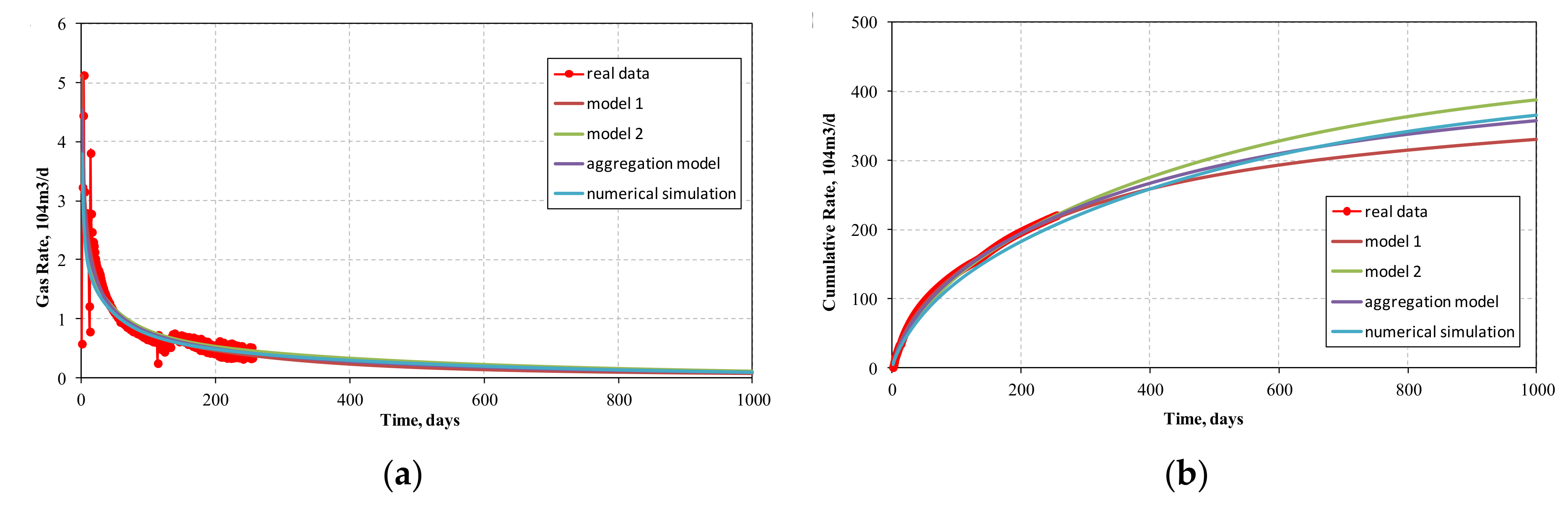
Thus, the likelihood for those two models can be calculated based on the difference between the history data and predictive data (see Figure 7), where L1 = 23.06, L2 = 19.88. Furthermore, based on Equation (19), the weights for those two models are as follows: w1 = 0.54, w2 = 0.46. Finally, the aggregation model can be presented based on Equation (20). Although the history data (less than 300 days) is limited from the viewpoint of establishing the integrated model, this new model has the capacity to predict the rate and cumulative rate for this well (see Figure 8).
To validate this proposed integrated model, a numerical model is developed to simulate the performance within 1000 days. At the same time, the new model simultaneously predicts the rate and cumulative rate within 1000 production days. We can apparently find that the rate can perfectly match with each other, while the cumulative rate predicted from the aggregation model can approximately match with the results calculated from the numerical model. In addition, those two models can provide an approximate range for the cumulative rate. It has the potential of decreasing the uncertainty for the prediction of estimation ultimate recovery, especially for unconventional reservoirs where the transient flow regime lasts for extremely long time. Based on Equation (21), the standard deviations of the rate and cumulative rate are obtained as follows: SD[qt = 1000] = 0.012 × 10⁴ m3/day, SD[Gt = 1000] = 12.4 × 10⁴ m3. Therefore, this new aggregation model is a practical tool in terms of predicting shale gas and tight gas rate.
5. Conclusions
This paper presents two new simple models for shale gas reservoirs with multi-stage fractured horizontal well, where the USRV zone is regarded as a dual-porosity & dual-depletion system. The resulting solutions are more universal for conducting type curve analysis in homogeneous and naturally fractured reservoirs. Numerical simulation model is correspondingly developed to validate the semi analytical solutions.
Two characteristic parameters, the pore volume ratio and thickness ratio are defined to characterize the dual-depletion mechanism. A set of type curves is generated under different cases of those two parameters. Several regular regimes can be identified, such as bilinear flow, linear flow, and outer boundary-dominated flow, etc.
The Generalized Likelihood Uncertainty Estimation methodology is introduced to aggregate those two models to reduce the uncertainties on future performance forecast. The numerical simulation and field application further validate the new simplified aggregation model. This paper also demonstrates that the proposed uncertainty assessment protocol using statistical model averaging concepts (GLUE) is a robust method to quantify the uncertainty of production prediction and cumulative prediction.
Author Contributions
M.C. and Y.D. mainly conducted the calculation of hybrid coupled model, L.Z performed the analysis and discussion, and Yuele J. conducted the application of field example. The manuscript was improved and revised by Yueru J. All of the authors contribute to the paper writing.
Acknowledgments
The authors acknowledge a fund from National Science and Technology Major Project (2017ZX05019005-006) and the Guidance Fund of Northeastern Petroleum University (2016YDL-13, 2017YDL-10).
Conflicts of Interest
The authors declare no conflict of interest.
Appendix A. Details on Mathematical Model
Appendix A.1. Conceptual Model 1
Based on the assumptions mentioned in Section 2.1, a set of mathematical models are subsequently established. According to the principle of mass balance, the fundamental partial differential equation that governs fluid flow is given as,
- For hydraulic fracture: diffusivity equation that control HF-horizontal well communication is described as
- For Natural fracture: diffusivity equation that control NF-HF communication is described as
- For sub-matrix 1: diffusivity equation that control matrix-HF communication is described as
- For sub-matrix 2: diffusivity equation that control matrix-NF communication is described as
Appendix A.2. Conceptual Model 2
In Upper Layer, the pressure governing equations in hydraulic fracture (HF), natural fracture (NF) and sub matrix 2 are given as:
In Lower Layer, the pressure governing equations in hydraulic fracture (HF), natural fracture (NF) and sub matrix 1 are given as:
Appendix A.3. Initial and Boundary Condition
In addition, initial conditions in HF, NF and matrix are given as:
- In model 1, inner boundary conditions are given as:
- In model 2, inner boundary condition in HF, NF and matrix are given as:
- In model 1 and model 2, outer boundary conditions in HF, NF and matrix are given as:
Appendix B. Constant Pressure Solution
Appendix B.1. Dimensionless Model in Laplace Domain
After using dimensionless definitions and Laplace transform to deal with Equations (A1)–(A14), the diffusion equations could be rewritten in the Laplace domain:
Appendix B.1.1. Model 1
The pressure governing equations in hydraulic fracture (HF), natural fracture (NF), matrix 1 and matrix 2 are list as follows:
In addition, the inner and outer boundary conditions are satisfied as:
Appendix B.1.2. Model 2
In the unit of upper layer, the pressure governing equations in hydraulic fracture, natural fracture and matrix 2 are given as:
In the unit of lower layer, the pressure governing equations in hydraulic fracture, natural fracture and matrix 1 are given as:
In addition, the inner and outer boundary conditions are satisfied as:
Appendix B.2. Laplace-Domain Solution
In the following section, the above equations of model 1 and model 2 are respectively solved in Laplace space.
Appendix B.2.1. Model 1
The general solution for Equations (A17) and (A18) can be obtained as follows:
After using boundary condition, the special solution for matrix 1 and matrix 2 is given as:
Similarly, the solution of governing equations of natural fracture also has the same formation. With the boundary condition, the final solution is as follows:
where
Similarly, the solution of governing equations of natural fracture also has the same formation. With the boundary condition, the final solution is as follows:
where
Based on the relationship between dimensionless pseudo pressure and dimensionless production, the rate can be presented as follows:
Appendix B.2.2. Model 2
Similarly, the solution of governing equations of model 2 also has the same formation like model 1. Because of the limitation of this paper, the pseudo pressure of hydraulic fracture is respectively presented for upper layer and lower layer.
In upper Layer, the dimensionless rate is presented as follows:
where
In lower layer, the dimensionless rate is presented as follows:
In terms of conceptual model 2, the total production rate is the sum of upper layer and upper layer, therefore, the final solution of production rate combing Equations (A36) and (A39):
References
- Clarkson, C.R. Production data analysis of unconventional gas wells: Review of the theory and best practices. Int. J. Coal Geol. 2013, 109, 101–149. [Google Scholar] [CrossRef]
- Nobakht, M.; Clarkson, C.R.; Kaviani, D. New type curves for analyzing horizontal well with multiple fractures in shale gas reservoir. J. Natl. Gas Sci. Eng. 2013, 10, 99–112. [Google Scholar] [CrossRef]
- Ozkan, E.; Brown, M.; Raghavan, R.; Kazemi, K.H. Comparison of fractured horizontal well performance in tight sand and shale gas reservoirs. SPE Reserv. Eval. Eng. 2011, 14, 248–259. [Google Scholar] [CrossRef]
- Stalgorova, E.; Mattar, L. Practical model to simulate production of horizontal wells with branch fractures. In Proceedings of the SPE Canadian Unconventional Resource Conference, Calgary, AB, Canada, 30 October–1 November 2012. [Google Scholar]
- Stalgorova, E.; Mattar, L. Analytical model for history matching and forecasting production in multi-fractured composite systems. In Proceedings of the SPE Canadian Unconventional Resource Conference, Calgary, AB, Canada, 30 October–1 November 2012. [Google Scholar]
- Weng, X.; Kressem, O.; Cohen, C.; Wu, R.; Gu, H. Modeling of hydraulic fracture network propagation in a naturally fractured formation. In Proceedings of the SPE Hydraulic Fracturing Conference and Exhibition, The Woodlands, TX, USA, 24–26 January 2011. [Google Scholar]
- Tan, L.; Zuo, L.; Wang, B. Methods of Decline Curve Analysis for Shale Gas Reservoirs. Energies 2018, 11, 552. [Google Scholar] [CrossRef]
- Wu, K.; Olson, J.E. Simultaneous multifracture treatments: Fully coupled fluid flow and fracture mechanics for horizontal wells. SPE J. 2015, 20, 337–346. [Google Scholar] [CrossRef]
- Zuo, L.; Yu, W.; Wu, K. A fractional decline curve analysis model for shale gas reservoirs. Int. J. Coal Geol. 2016, 163, 140–148. [Google Scholar] [CrossRef]
- Li, Y.; Zuo, W.; Yu, W.; Chen, Y. A Fully Three Dimensional Semianalytical Model for Shale Gas Reservoirs with Hydraulic Fractures. Energies 2018, 11, 436. [Google Scholar] [CrossRef]
- Barenblatt, G.I.; Zhelto, I.P.; Kochina, I.N. Bacis Concepts of the theory of Seepage of Homogeneous Liquids in Fissured Rocks. J. Appl. Math. Mech. 1960, 24, 852–864. [Google Scholar] [CrossRef]
- Warren, J.E.; Root, P.J. The Behavior of Naturally Fractured Reservoirs. SPE J. 1963, 3, 245–255. [Google Scholar] [CrossRef]
- Kazemi, H. Pressure Transient of Naturally Fractured Reservoirs with Uniform Fracture Distribution. SPE J. 1969, 12, 451–462. [Google Scholar] [CrossRef]
- De Swaan, O.A. Analytical Solution for Determining Naturally Fractured Reservoir Properties by Well Testing. SPE J. 1976, 12, 117–122. [Google Scholar] [CrossRef]
- Ozkan, E.; Raghavan, R. Some applications of pressure derivative analysis procedure. In Proceedings of the 62nd Annual Technical Conference and Exhibition, Dallas, TX, USA, 27–30 September 1987. [Google Scholar]
- Al-Ghamdi, A.; Ershaghi, I. Pressure Transient Analysis of Dually Fractured Reservoirs. SPE J. 1996, 2, 23–25. [Google Scholar] [CrossRef]
- Liu, J.C.; Bodvarsson, G.S.; Wu, Y.S. Analysis of Flow Behavior in Fractured Lithophysal Reservoirs. J. Contam. Hydrol. 1996, 62–63, 189–211. [Google Scholar] [CrossRef]
- Wu, Y.S.; Liu, H.H.; Bodvarsson, G.S. A Triple-Continuum Approach for Modeling Flow and Transport Process in Fractured Rock. J. Contam. Hydrol. 2004, 73, 145–179. [Google Scholar] [CrossRef] [PubMed]
- Dreier, J. Pressure Transient Analysis of Wells in Reservoirs with a Multiple Fracture Network. Master’s Thesis, Colorado School of Mines, Golden, CO, USA, 2004. [Google Scholar]
- El-Banbi, A.H. Analysis of Tight Gas Wells. Ph.D. Thesis, Texas A&M University, College Station, TX, USA, 1998. [Google Scholar]
- Al-Ghamdi, A.; Chen, B.; Behmanesh, H.; Qanbari, F.; Aguilera, R. An improved triple-porosity model for evaluation of naturally fractured reservoir. SPE Reserv. Eval. Eng. 2011, 8, 397–404. [Google Scholar] [CrossRef]
- Zhao, Y.L.; Zhang, L.H.; Wu, F. Analysis of horizontal well pressure behavior in fractured low permeability reservoirs with consideration of threshold pressure gradient. J. Geophys. Eng. 2013, 10, 1–10. [Google Scholar] [CrossRef]
- Obinna, E.D.; Hassan, D. A model for simultaneous matrix depletion in natural and hydraulic fracture network. J. Natl. Gas Sci. Eng. 2014, 16, 57–69. [Google Scholar]
- Tian, L.; Xiao, C. Well testing model for multi-fractured horizontal well for shale gas reservoir with consideratuon of dual diffusion in matrix. J. Natl. Gas Sci. Eng. 2014, 21, 283–295. [Google Scholar] [CrossRef]
- Stehfest, H. Numerical inversion of Laplace transforms-algorithm 368. Commun. ACM 1970, 13, 47–49. [Google Scholar] [CrossRef]
- Rasheed, O.; Bello, R.; Wattenbarger, A. Rate Transient analysis in naturally fractured shale gas reservoirs. In Proceedings of the CIPC/SPE Gas Technilogy Symposium 2008 Joint Conference, Calgary, AB, Canada, 16–19 June 2008. [Google Scholar]
- Beven, K.J.; Binley, A. The future of Distribution Models: Model Calibration and Uncertainty Prediction. Hydrol. Process 1992, 6, 278–289. [Google Scholar] [CrossRef]
Figure 1.
(a) The illustration of multi-fractured horizontal well; (b) The two segments of matrix in stimulated reservoir volume (SRV) zone.
Figure 1.
(a) The illustration of multi-fractured horizontal well; (b) The two segments of matrix in stimulated reservoir volume (SRV) zone.
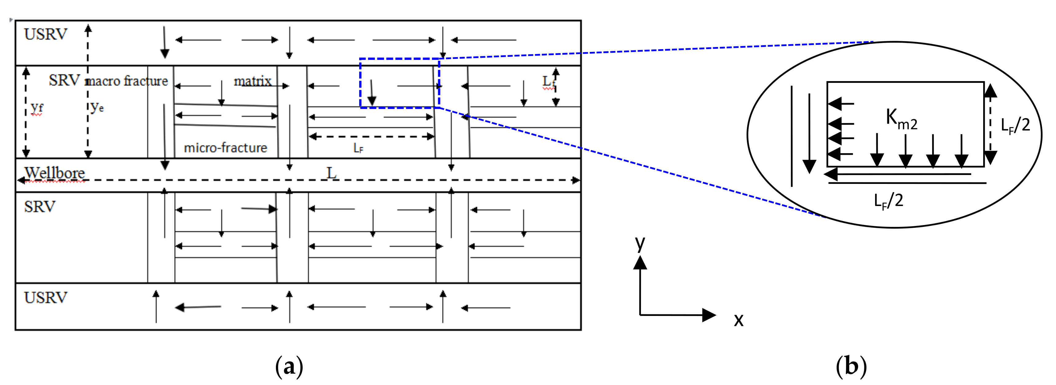
Figure 2.
Two new conceptual models of matrix: (a) conceptual model 1; (b) conceptual model 2.

Figure 3.
Comparison of our model with alternative analytical approach in the dimensionless coordinate.
Figure 3.
Comparison of our model with alternative analytical approach in the dimensionless coordinate.

Figure 4.
(a) Depleted shale gas reservoir model established using Eclipse 2010; (b) Comparison between numerical model and those two new models proposed in this paper.
Figure 4.
(a) Depleted shale gas reservoir model established using Eclipse 2010; (b) Comparison between numerical model and those two new models proposed in this paper.

Figure 5.
Type curve of flow regime: (a) Cartesian plot for model 1; (b) log-log plot for model 1; (c) Cartesian plot for model 2; (d) log-log plot for model 2.
Figure 5.
Type curve of flow regime: (a) Cartesian plot for model 1; (b) log-log plot for model 1; (c) Cartesian plot for model 2; (d) log-log plot for model 2.

Figure 6.
Natural seismic event for this well, where the spots with different color stand for the individual stages.
Figure 6.
Natural seismic event for this well, where the spots with different color stand for the individual stages.
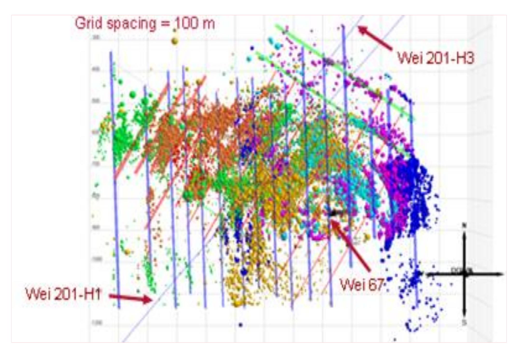
Figure 7.
Two models match with the field data: (a) rate vs. t, model 1; (b) cumulative rate vs. t, model 1; (c) rate vs. t, model 2; (d) cumulative rate vs. t, model 2.
Figure 7.
Two models match with the field data: (a) rate vs. t, model 1; (b) cumulative rate vs. t, model 1; (c) rate vs. t, model 2; (d) cumulative rate vs. t, model 2.
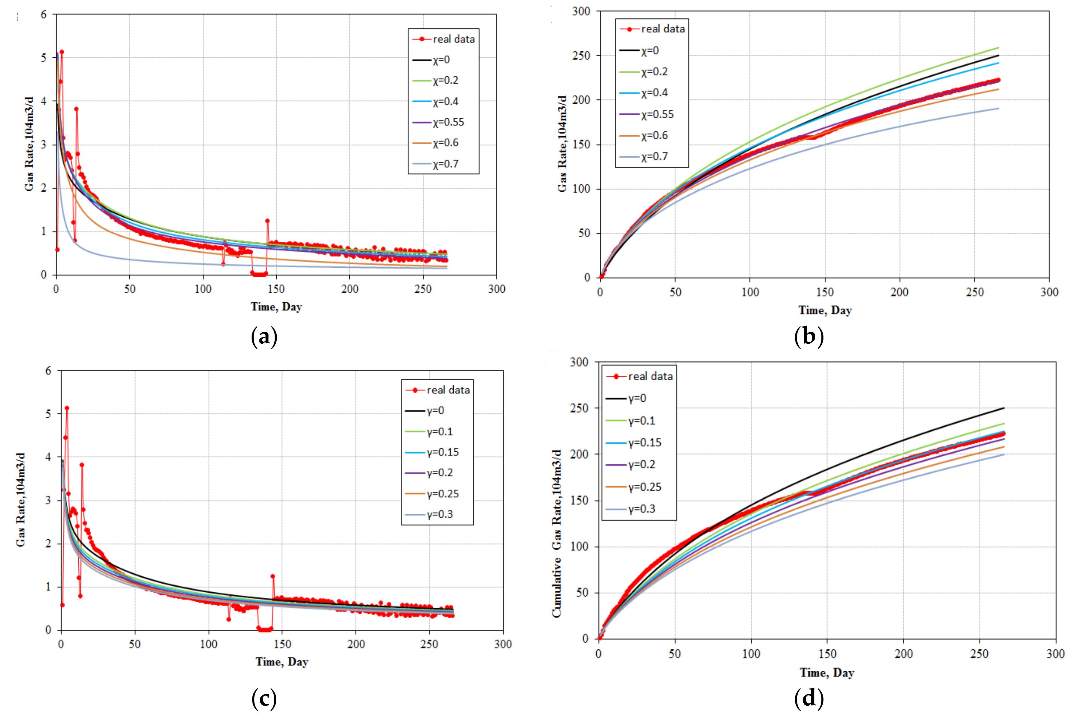
Figure 8.
Comparison between aggregation model and numerical simulation: (a) gas rate; (b) cumulative rate.
Figure 8.
Comparison between aggregation model and numerical simulation: (a) gas rate; (b) cumulative rate.


Table 1.
Definition of dimensionless variables.
| Dimensionless Variables | Definitions |
|---|---|
| Dimensionless pseudo pressure | , where |
| Dimensionless time | , |
| Dimensionless space | , , |
| Dimensionless inter-porosity index | , , |
| Dimensionless storability ratio | , where |
| Dimensionless conductivity ratio | |
| Dimensionless production data | |
| Dimensionless permeability ratio |
Table 2.
Qualitative description of initial and boundary conditions.
| Condition | Model 1 | Model 2 | |
|---|---|---|---|
| Initial | |||
| Inner boundary | HF | ||
| NF | , | , , | |
| Matrix | , , | , , | |
| Outer boundary | , , | ||
Table 3.
Input parameters used in the case of constant flowing pressure.
| Parameters | Symbol | Unit | Value |
|---|---|---|---|
| Initial pressure | Pi | MPa | 20 |
| Downhole pressure | Pwf | MPa | 15 |
| Formation temperature | T | K | 333 |
| Horizontal length | L | m | 1200 |
| Formation thickness | H | m | 100 |
| Macro-fracture length | yf | m | 200 |
| Total compressibility of HF | CtF | MPa−1 | 5 × 10⁻⁴ |
| Total compressibility of NF | CtF | MPa−1 | 5 × 10⁻⁴ |
| Total compressibility of Matrix | CtF | MPa−1 | 5 × 10⁻⁴ |
| Porosity of HF | ΦF | Dimensionless | 0.0005 |
| Porosity of NF | Φf | Dimensionless | 0.005 |
| Total porosity of matrix | Φm | Dimensionless | 0.08 |
| Permeability of HF | kF | D | 2 |
| Permeability of natural fracture | kf | D | 10−6 |
| Permeability of sub-matrix m1 | km1 | D | 10−8 |
| Permeability of sub-matrix m2 | km2 | D | 10−8 |
| Langmuir pressure | PL | MPa | 5 |
| Langmuir volume | VL | sm3/m3 | 5 |
Table 4.
Input parameters used in the field example.
| Parameters | Symbol | Unit | Value |
|---|---|---|---|
| Initial pressure | Pi | MPa | 22.5 |
| Downhole pressure | Pwf | MPa | 15 |
| Formation temperature | T | K | 314 |
| Horizontal length | L | m | 1450 |
| Formation thickness | H | m | 48.3 |
| Macro-fracture length | yf | m | 214 |
| Total compressibility of HF | CtF | MPa−1 | 5.2 × 10⁻⁴ |
| Total compressibility of NF | CtF | MPa−1 | 5.2 × 10⁻⁴ |
| Total compressibility of Matrix | CtF | MPa−1 | 5.2 × 10⁻⁴ |
| Porosity of HF | ΦF | Dimensionless | 4.6 × 10⁻⁴ |
| Porosity of NF | Φf | Dimensionless | 5.3 × 10⁻³ |
| Total porosity of matrix | Φm | Dimensionless | 0.078 |
| Permeability of HF | kF | D | 1.8 |
| Permeability of natural fracture | kf | D | 2.1 × 10⁻⁶ |
| Permeability of sub-matrix m1 | km1 | D | 1.2 × 10⁻⁸ |
| Permeability of sub-matrix m2 | km2 | D | 1.2 × 10⁻⁸ |
| Langmuir pressure | PL | MPa | 5.2 |
| Langmuir volume | VL | sm3/m3 | 5.2 |
© 2018 by the authors. Licensee MDPI, Basel, Switzerland. This article is an open access article distributed under the terms and conditions of the Creative Commons Attribution (CC BY) license (http://creativecommons.org/licenses/by/4.0/).
Share and Cite
MDPI and ACS Style
Cao, M.; Dai, Y.; Zhao, L.; Jia, Y.; Jia, Y. Hybrid Coupled Multifracture and Multicontinuum Models for Shale Gas Simulation by Use of Semi-Analytical Approach. Energies 2018, 11, 1308. https://doi.org/10.3390/en11051308
AMA Style
Cao M, Dai Y, Zhao L, Jia Y, Jia Y. Hybrid Coupled Multifracture and Multicontinuum Models for Shale Gas Simulation by Use of Semi-Analytical Approach. Energies. 2018; 11(5):1308. https://doi.org/10.3390/en11051308
Chicago/Turabian StyleCao, Maojun, Yu Dai, Ling Zhao, Yuele Jia, and Yueru Jia. 2018. "Hybrid Coupled Multifracture and Multicontinuum Models for Shale Gas Simulation by Use of Semi-Analytical Approach" Energies 11, no. 5: 1308. https://doi.org/10.3390/en11051308
Note that from the first issue of 2016, this journal uses article numbers instead of page numbers. See further details here.