Zero-Axis Virtual Synchronous Coordinate Based Current Control Strategy for Grid-Connected Inverter

School of Electrical and Power Engineering, China University of Mining and Technology, Xuzhou 221116, China
*
Author to whom correspondence should be addressed.
Energies 2018, 11(5), 1225; https://doi.org/10.3390/en11051225
Submission received: 12 April 2018
/
Revised: 9 May 2018
/
Accepted: 9 May 2018
/
Published: 10 May 2018
(This article belongs to the Section F: Electrical Engineering)
Abstract
:Unbalanced power has a great influence on the safe and stable operation of the distribution network system. The static power compensator, which is essentially a grid-connected inverter, is an effective solution to the three-phase power imbalance problem. In order to solve the tracking error problem of zero-sequence AC current signals, a novel control strategy based on zero-axis virtual synchronous coordinates is proposed in this paper. By configuring the operation of filter transmission matrices, a specific orthogonal signal is obtained for zero-axis reconstruction. In addition, a controller design scheme based on this method is proposed. Compared with the traditional zero-axis direct control, this control strategy is equivalent to adding a frequency tuning module by the orthogonal signal generator. The control gain of an open loop system can be equivalently promoted through linear transformation. With its clear mathematical meaning, zero- sequence current control can be controlled with only a first-order linear controller. Through reasonable parameter design, zero steady-state error, fast response and strong stability can be achieved. Finally, the performance of the proposed control strategy is verified by both simulations and experiments.
1. Introduction
Electric energy is a kind of clean energy which is convenient for transmission. It has many advantages, such as high energy utilization and flexible and convenient use. With the complex and intelligent development of the power grid, the uneven distribution of the time-varying single-phase load has caused uneven distribution of the three-phase load, thus resulting in unbalanced three-phase current and extra neutral point current [1,2]. Unbalanced power has a great influence on the safe and stable operation of the distribution network system, causing additional losses of the line [3], increasing the losses of distribution transformers [4] and reducing the efficiency of motors [5].These will lead to the loss and waste of electric energy.
A number of methods have been proposed to solve three-phase unbalanced power problems in distribution networks. Phase-change switches adopting permanent magnet relays to commutate operations were the earliest method [6]. However, there were both an arc and a voltage drop in switching operations, which had a great impact on lines and switches [7]. Recently, the unbalanced power suppression method is interphase capacitor, utilizing the characteristic angles of capacitance line current vectors and phase voltage vectors to realize the transfer of active power and reactive power [8], but the active power transfer capacity of the method is relatively small, and the active power is regulated while reactive power imbalance comes into being. With the maturity of power electronic inverter technology, an active static power compensator (SPC) [9,10] has appeared. The inverter device works as a controlled current source, which outputs the unbalanced current in the active form to counteract the unbalanced fundamental current produced by the load. The three-phase power flowing into the upper level transformer can be adjusted and balanced [11]. Due to the advantages of excellent unbalanced current compensation, no voltage drop and no reactive power transfer, it has gradually become a research hotspot in the field of unbalanced power management.
With the characteristics of high DC voltage utilization and small DC voltage ripple, three-phase four-leg grid-connected inverters [12] are considered a common structure of SPC [13]. When the three-phase negative- and zero-sequence current signals are transformed into reference signals in the synchronous rotating coordinate frame, the reference signals in dq0-axis are all AC signals. Generally, the first-order controller cannot track the AC reference signal with zero steady-state error and the existence of switch dead zones further reduces the open loop gain, resulting in imperfect compensation.
To solve the problem of AC signal tracking, many improved control algorithms have been developed. Dead time compensation [14] is a traditional way of compensation. However, due to the complexity of the compensation algorithm and high detection requirements, this method has gradually been less used at the present stage. Recently the general method is to improve the control algorithm and directly use the controller to improve the tracking performance. The commonly used methods can be divided into four categories. The first method is adopting the first-order controller to achieve the tracking control of type-I system with zero steady-state error, by reducing the frequency of the controlled signal to DC [15]. Among these, the most classical control scheme is the dual synchronous rotation axis control [16]. Through the design of negative-sequence synchronous coordinate axes, the frequency of negative-sequence signal can be reduced and tracked, but this method is only suitable for three-phase systems. The second way is to improve the control gain and reduce the steady-state error by increasing the open loop gain. Resonant control [17] is a typical control algorithm. In [18], the instantaneous power error tracking of voltage source inverter has been realized by resonant control. According to desired transient behavior of AC or AC? Be consistent signal amplitude, a method for deriving PR controller structures and coefficients has been proposed in [19], based on the fact that an AC signal envelope is perceived as a DC signal. However, in discrete applications, the resonance point of this method may drift. It is necessary to introduce phase locked frequency and phase compensation, yet by doing so the complexity of the calculations is increased. The third method is to apply an internal model principle to model external signals. The error signal is accumulated to increase the open loop equivalent gain of the control system, so as to reduce the steady-state error of the closed-loop system. As a kind of internal model control, repetitive control has been applied to accumulate output deviations to input and improve the tracking ability of fixed frequency AC signals in [20,21]. The tracking performance of the method is excellent for periodic input signals. However, for aperiodic fast changing signals, the tracking performance is ineffective. Predictive control or deadbeat control have been adopted to improve the dynamic and steady state performance of the system [22,23]. It is worth noting that this method is excessively dependent on the availability of a precise model, which limits its application. The fourth kind of methods is the nonlinear control, such as sliding mode variable structure control [24,25], which has been applied to the control of three-phase four-leg inverters, but nonlinear control is usually complicated in structure and difficult to implement.
In this paper, a novel zero-axis current reconfiguration control algorithm is proposed to solve the problem of zero-axis current signal tracking. According to the positive-, negative- and zero-sequence signal extracting matrixes, the frequency domain phase shifting coefficient s is used to construct first-order filter matrices of three phase sequences. With the proposed orthogonal signal generator (OSG) based on the filter transmission matrix, the zero-axis signal is reconstructed by linear transformation. Moreover the zero-axis virtual synchronous coordinate system is constructed, in which the current control is carried out. The working characteristics of the designed control system are analyzed in the time domain and frequency domain and the parameters of the zero-axis virtual orthogonal generator and controller are analyzed through pole assignment. The proposed method, which has a clear mathematical meaning, can realize virtual mapping and high gain tracking of zero-axis current. Results of both simulations and experiments show that this method has zero steady-state error, fast response performance and strong stability.
2. Principle Analysis of SPC
2.1. Unbalance Current Analysis
On the basis of the Lyon’s algorithm [26], the positive-, negative- and zero-sequence parts of the fundamental current can be expressed as:
where stands for the 120° shift coefficient of three-phase time domain signals. After the conversion to αβγ stationary coordinate system, the positive- and negative-sequence fundamental current are coupled, respectively. The zero-sequence component is independent in the γ-axis (i.e., iγ).
By transforming the current vectors from abc coordinate system to the αβγ coordinate system, the three phase sequence fundamental signals can be written as:
where denotes the generalized Clarke transform, and stands for the 90° shift coefficient of αβγ coordinate system.
Mapped to the synchronous rotating coordinate system, the positive- and the negative-sequence signals convert to polar coordinate signals. Through the stationary-to-synchronous frame transformation, the former turns into a DC signal, and the latter turns into a frequency multiplication signal, respectively. Different from the axis of rotation, the zero-axis is a fixed one, which means can be directly obtained without signal frequency increasing and decreasing.
2.2. Compensation Principle of SPC
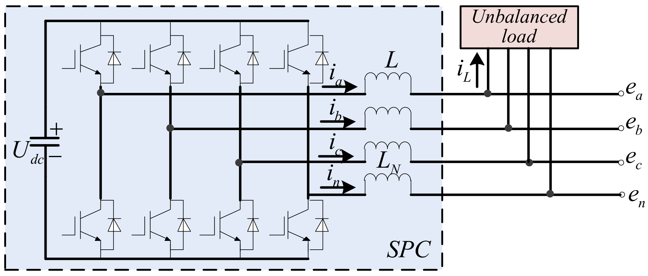
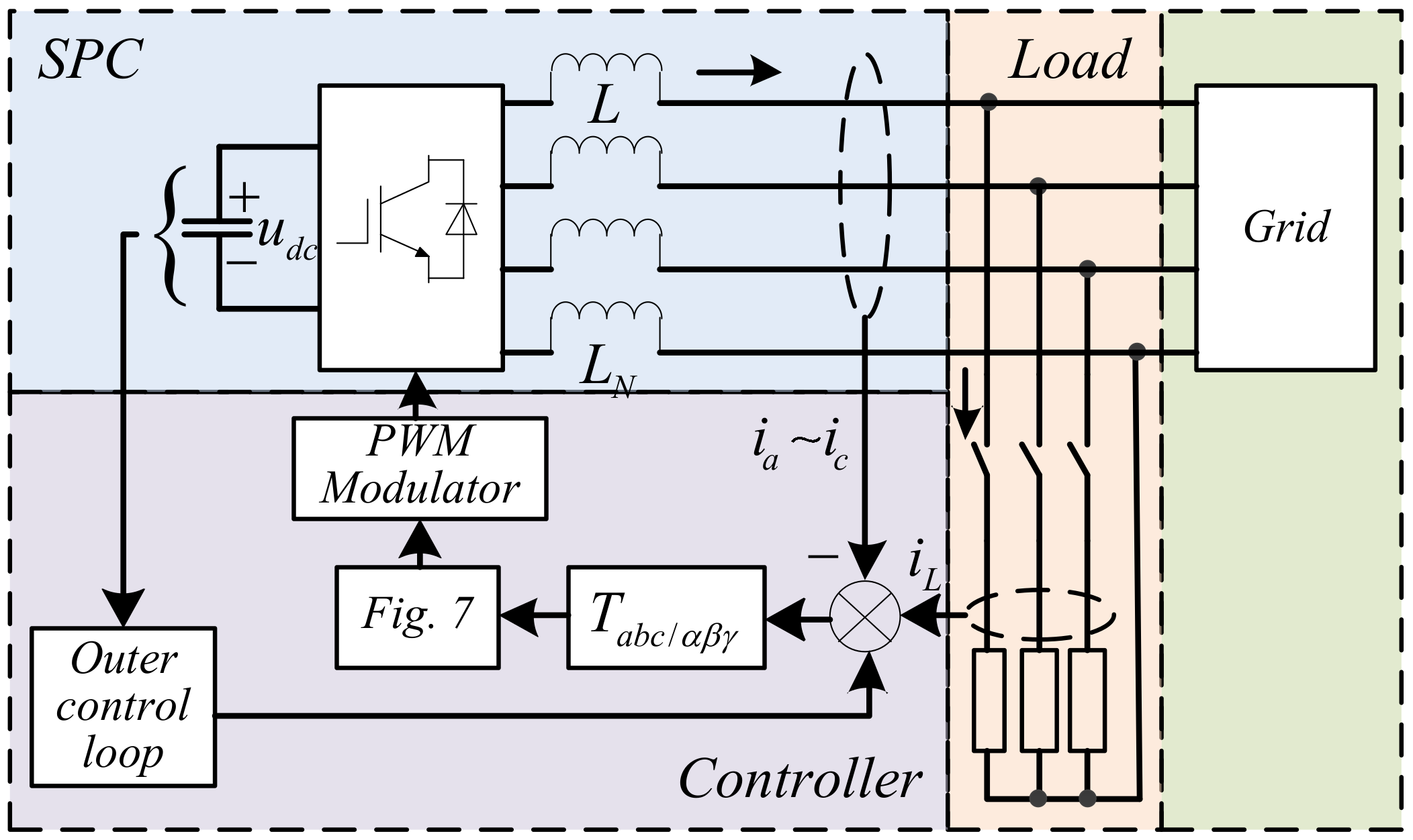
The SPC is a three-phase four-leg grid connected inverter, which is in parallel with the unbalanced load. Detecting the negative- and zero-sequence component of the load current, the device counteracts the unbalanced current component through the output of the compensation current with the same amplitude and the opposite phase. The structure is shown in Figure 1.
Ignoring the equivalent series resistance of the inductor, the system model in synchronous rotating coordinate axis can be described as:
where the inductor current of the inverter is state variable, the output voltage of the inverter is the control volume, and the grid voltage is the feed forward interference. The control coefficient and the coupling coefficient are expressed as:
Although the first item on the right side of the Equation (3) is a coupling one, it can be decoupled by state variable cross feed-forward. After decoupling, the three state variables are relatively independent, which means three independent controllers are needed for control.
3. Current Control Strategy Based on Zero-Axis Signal Reconstruction
3.1. Design of the Virtual Zero-Axis Coordinate System
In order to achieve zero-axis current control, a virtual zero-axis coordinate system is built on the plane perpendicular to the dq plane. In order to facilitate analysis, the plane composed of q-axis and zero-axis as the target plane is chosen, which is defined as a 0d-0q plane.
First, choosing the original zero-axis and the inverse vector direction of q-axis as the coordinate axis, the 0α-0β coordinate system can be constructed. The direction of 0α-axis is the same as that of original zero-axis, and the signal in 0α-axis is original zero-sequence signal. The 0β-axis is the reverse vector direction of the original q-axis, and the signal in 0β-axis is the virtual zero-axis orthogonal signal.
Based on this coordinate system, a 0d-0q virtual synchronous coordinate system is designed. Define the plane corresponding to the positive direction of the d-axis as the observation plane. Then the numerical relationship between virtual synchronous coordinate system and static coordinate system can be written as:
where is the output angle of the system phase-locked loop. The virtual synchronous coordinate system of fundamental frequency and counter clockwise rotation can be obtained as shown in Figure 2.
In order to achieve zero-axis signal reconstruction, the virtual orthogonal signal of zero-axis current needs to be constructed.
3.2. Complex Filter Matrixes Transformation
From Equations (2a)–(2c), we know that in the αβγ coordinate system, the positive-, negative- and zero sequence signals can be expressed as the matrix operation of the phase shift coefficient. Therefore a similar virtual αβγ coordinate system can be constructed in zero-axis.
For this purpose, a class of first-order positive-, negative- and zero-sequence filters [27] are introduced as shown in (6):
where stands for the measured value of the fundamental frequency, and stands for the cut-off frequency of the low pass filter.
The fundamental positive-sequence signal can pass through the without phase deviation and attenuation. And for the signals at other frequencies, there will be certain attenuation. The characteristics of negative-sequence filter are similar to the former. In addition, zero-sequence filter is the traditional first-order inertial element.
Respectively, the corresponding three third-order diagonal matrices can be written as , , and .
By replacing phase shift coefficient in (2a)–(2c) with the 90° shift coefficient in frequency domain (i.e., j), the phase shift matrixes based on Clarke transformation can be established as , , and .
Subsequently, the filter matrixes based on generalized Clarke transform can be constructed in the complex frequency domain as follows:
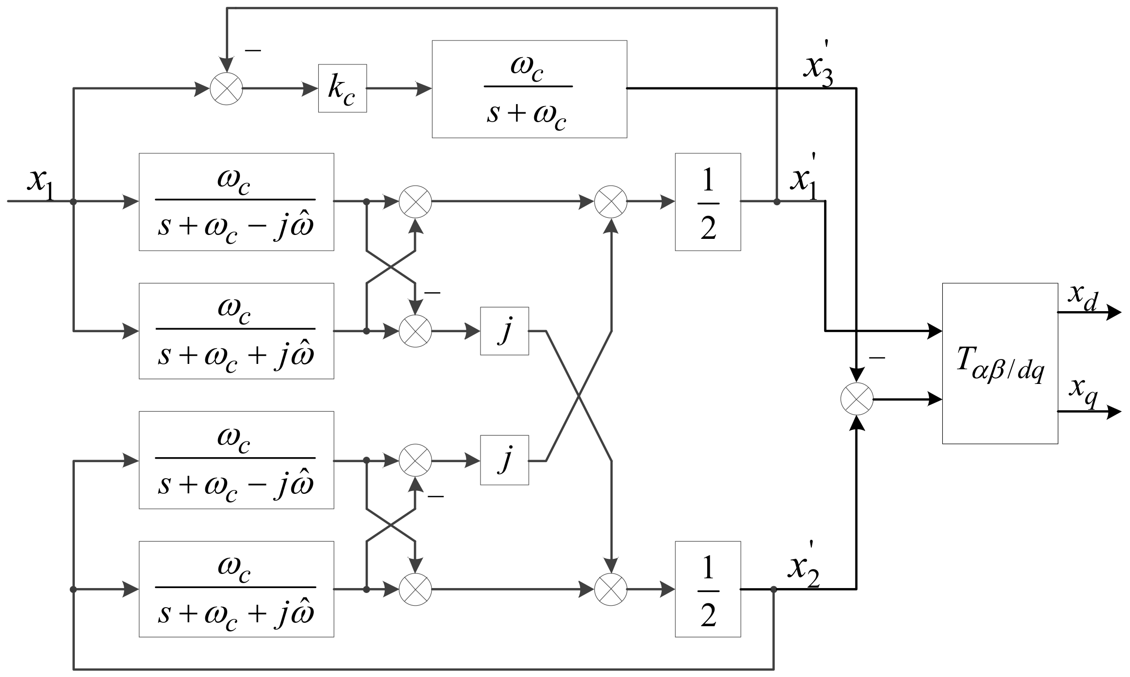
In order to achieve zero-sequence signal transformation and linear transformation, a signal processing module based on filter matrixes is designed. Assume that x1, x2 and x3 denote the module signal inputs, and x1’, x2’ and x3’ denote the outputs. With the linear combination of filter matrixes, the module can be calculated as:
where .
By feeding the output to input, (8) can be set as , . The filter transfer matrixes model is shown in Figure 3 with the output signal feedback.
Equation (8) can be transformed into (9):
and then, through feedback and calculation, a simpler form is obtained with the imaginary part eliminated. The transfer function of the single-input three-output system can be calculated as:
On the basis of the sequence numerical relationship in Lyon's method, the filter transmission matrices module transforms the original zero-axis signal in the frequency domain. Define the input of the single input system as the original zero-axis signal. Then the transfer function (10) is equivalent to the establishment of a virtual coordinate system through the phase shift matrixes. And the zero-axis signal can be controlled in the new coordinate system through the linear transformation.
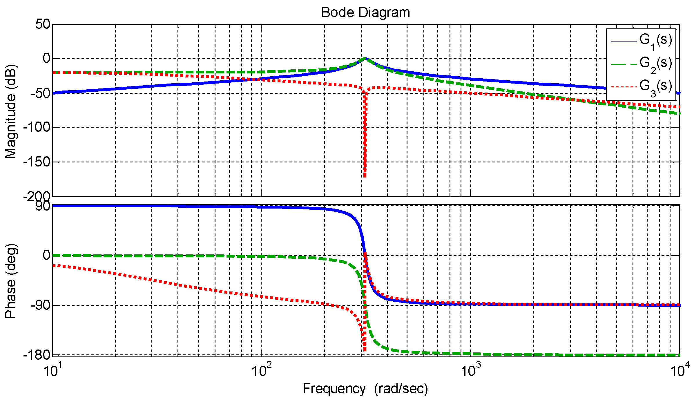
Assume the fundamental frequency as 50 Hz and the cut-off frequency of the low pass filter as 5 Hz. The frequency characteristics of the filter transmission matrixes can be obtained as shown in Figure 4.
From Figure 4, we can see that G1(s) has the characteristic of the band pass filter. There are no phase deviation and attenuation at . However it has strong attenuation effect on other frequency signals. Selecting the fundamental frequency of the power grid as the center frequency, the harmonic component can be suppressed, and the fundamental signal can pass through without attenuation. G2(s) exhibits a low pass filter behavior, with no amplitude attenuation and 90° phase lag at . And it has a strong attenuation effect on the signal larger than the frequency. G3(s) exhibits a band resistance behavior. The amplitude frequency characteristic and phase frequency characteristic of low frequency band are similar to G2(s). However, it attenuates rapidly at with strong attenuation effect on the signal of higher frequency. Therefore, based on Equation (9), we can realize the function of band pass by , with the attenuation of low frequency part in orthogonal signal.
The constructed matrix signal processing module produces a signal that is orthogonal to the specific frequency of the original signal, which is defined as the filter transmission matrixes orthogonal signal generator (FTM-OSG).
3.3. Design of Zero-Axis Control System
In the expectation plane, two-phase virtual static coordinate system is constructed to reconstruct the original zero-axis signal as follows:
The two terms in the matrix denote the transfer function from x0(s) to x0α(s) and x0β(s), which can be expressed as G0α(s) and G0β(s).
With the virtual coordinate system added, the original dq0 three-axis control system is transformed into the dq-0d0q four-axis control system. The amplitude, frequency and phase information of sinusoidal reference signals in the fixed zero-axis are extracted with matrix transformation, and the signals are transformed to a pair of orthogonal polar coordinate signals. On the new coordinate frame, the frequency and phase information of the controlled object have been pre-extracted. The controller only needs to control the steady-state accuracy and response speed of amplitude tracking. It is equivalent to increasing the freedom degree of control system through linear transformation with no more input information.
On the basis of the established zero-axis virtual coordinate system, the reference current and device current are mapped to the virtual synchronous coordinate system for control. The zero-axis reference current is the load zero-sequence fundamental current, which can be extracted from the zero-sequence current by FTM-OSG.
According to (5), the load zero-sequence fundamental current can be mapped to the virtual rotating coordinate system. The single-input and double-output system is shown in Figure 5.
The SPC is a typical current tracking system. For zero-sequence current, the control requirement is that reference current can be completely tracked at the fundamental frequency with small harmonic component. Considering that zero-axis current control does not affect DC voltage control, zero-axis current control system can be built as shown in Figure 6. In the figure, − represents Laplace transform of Park transform and G0(s) denotes zero-axis current transfer function.
For the fundamental signal tracking, the control system is a single closed loop control system with two controllers. Compared with the traditional zero-axis direct control, this control strategy is equivalent to adding frequency tuning module by the orthogonal signal generator. Through linear coordinate transformation, the original system tracking problem is converted to the origin stabilization problem of the new system. Therefore the control objective of the system is to find a suitable control law to make it asymptotically stable at and ensure good dynamic and steady state performance.
In Figure 6, the output of the controller contains the zero-axis real current tracking control signal and the orthogonal virtual current tracking signal. In the synchronous rotating coordinate system, there is a coupling relationship between the two signals. In order to realize the decoupling of the real control signal and the virtual one, the signal should be converted to the stationary coordinate system. And the decoupled signal on the 0α-axis is taken as the real control signal.
With this linear transformation and decoupling done, the new closed loop system is still a linear system through the inverse transformation. The controller can be designed for the new linear system to achieve the control function of the original zero-axis system.
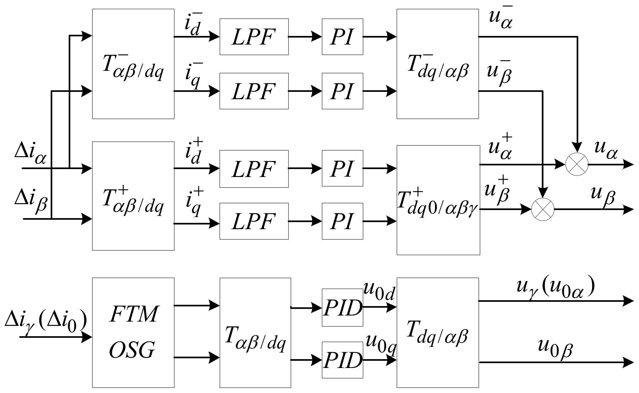
The double synchronous coordinate control scheme is adopted as the positive- and negative-sequence fundamental current control. And the control block diagram of SPC is as shown in Figure 7.
4. Analysis and Design of the Zero-Axis Control System
4.1. State Space Analysis of Zero-Axis Virtual Coordinate System
Considering the fundamental component only, the control system in Figure 5 can be described as the form of state equation. Define v as input, x as state variable, y as output variable. The zero-axis signal virtual mapping system can be expressed as:
According to (12), the zero-axis signal virtual mapping system is a linear system. The dynamic response, stability and other performance depend on the low pass filter cut-off frequency and the phase locked loop output frequency .
Once the output of PLL is a constant, the system can be described as a linear time invariant system. According to the Caylay-Hamilton theorem, the local stability can be calculated as follows:
From (13), the eigenvalues of the system are calculated as:
The three eigenvalues are all negative, indicating that the system is both internally and externally stable. The zero state response caused by the bounded input is bounded.
Define the zero-axis input signal as and the angular frequency as . When is as same as the input signal , the steady state solution of (12) can be obtained as follows:
4.2. Parameter Analysis of Zero-Axis FTM-OSG
Compared with the traditional zero-axis control mathematical model, the construction of a virtual orthogonal signal is added. Therefore not only the parameters of controller, but also the parameter of the zero-axis virtual FTM-OSG need to be determined.
According to (12), once the voltage frequency of the grid is determined, the performance of the virtual mapping system of zero-axis signal is only related to the low pass filter cut-off frequency . In order to achieve faster dynamic response and better filtering effect, it is necessary to optimize the parameter.
Based on the frequency characteristics of the FTM-OSG system, quality factor function (i.e., Q) of the filter link can be defined as the equation of the center frequency divided by the transfer function bandwidth (i.e., amplitude attenuation −3 dB). Selecting the center frequency as the fundamental frequency of the power grid, quality factor can be expressed as:
where BW represents the bandwidth of the transfer function. The tendency of the quality factor changing with the parameter is shown in Figure 8.
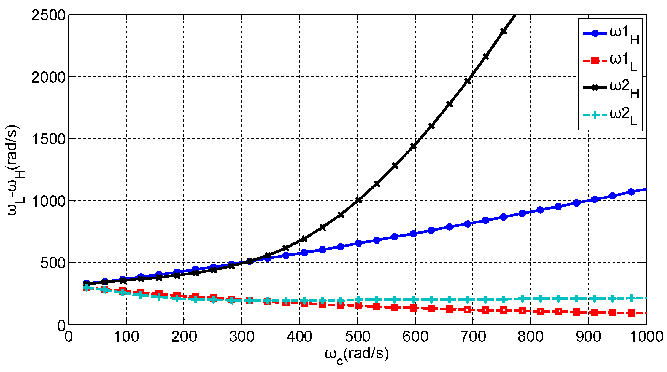
In Figure 8, Q1 and Q2 respectively represent the quality factors of the original signal extraction link and the orthogonal signal generation link. The corresponding upper bound frequency and lower bound frequency are shown in Figure 9.
As shown in Figure 8 and Figure 9, the bandwidth of the OSG module is determined by the cut-off frequency of the complex filters. The smaller value of corresponds to the smaller bandwidth and more excellent frequency selection performance. But the dynamic response speed is slow and the anti-interference is weak. The increase of the value can increase the bandwidth, the anti-interference ability and response speed of the system, at the cost of the attenuation rate decline. Therefore, filter parameter should be selected according to system requirements. Considering that the normal fluctuation of grid fundamental frequency is ±0.2 Hz, the limitation of parameter selection is .
On the other hand, the system characteristics can be analyzed from the perspective of eigenvalues. Based on transfer function (13), when , the eigenvalue distribution of the system under different values can be described as shown in Figure 10.
Generally the eigenvalues all have negative real parts, which indicate that the system is stable. The further the eigenvalue is from the imaginary axis, the faster the dynamic response of the system is. When the parameter increases from 0 to , the dominant eigenvalue of the system gets far away from the imaginary axis, indicating that the dynamic performance is enhanced. However, if the parameter continue increasing, the dominant eigenvalue of the system approaches the imaginary axis, which means that the dynamic response speed has reduced. In consideration of the frequency selection performance and response speed, we set it as .
4.3. Coordinate Transformation Analysis of Control System
In order to analyze the effectiveness of the virtual zero-axis control system, the open-loop characteristics need to be analyzed. With fundamental current control considered only, due to the existence of matrix transformation, the open-loop transfer function of the zero-axis control system can be expressed as the time domain matrix transformation:
Then the 0d-0q virtual synchronous coordinate system can be obtained through calculation and conversion as follows:
It can be seen that the signal on the 0d-0q virtual axis is obtained by the translation of the virtual stationary axis through the frequency domain translation and the matrix transformation. The dynamic transition time and the attenuation speed of dynamic term depend on the construction speed of the virtual orthogonal signal, as shown in Appendix A. Although the forward channel system can be analyzed at the equilibrium point of the virtual coordinate system, the signals in 0d-0q axis are strongly coupled. It cannot be linearized in the virtual synchronous coordinate system.
The systematic analysis is carried out directly in the 0α-0β coordinate system. Define the control signal output as . Then the control link can be expressed as:
By introducing the PID controller transfer function into (19), it can be rewritten as:
Assume that the controller contains an integral component, there will be a resonant link in the process of matrix transformation, which means there are conjugate poles with zero real part in the open loop transfer function of the system. The resonance poles can effectively increase the open loop gain at the characteristic frequency, with large amplitude attenuation at other frequencies. In addition, the integral constant only changes the attenuation degree of the resonance link at other frequency, rather than its bandwidth. When the system frequency fluctuation range is large, a small bandwidth means that the adaptability of frequency change is poor. Moreover the FTM-OSG has completed the extraction of the characteristic signal. The series correction link does not need to add more pole points in imaginary axis to increase the gain at the characteristic frequency. Therefore, the controller can be reduced to the PD controller.
Based on (11), (17) and (20), the expression of controller function can be obtained as:
The zero-axis control system is shown in Figure 11. In the figure, GPWM(s) denotes the transfer function of the converter PWM link. KPWM denotes the equivalent gain of this link. TPWM denotes the equivalent delay of the signal sampling and the PWM link, which is set to 1.5 times of the sampling period Ts. G0(s) is the four-leg inverter zero-axis transfer function. As shown in Figure 12, with the zero-sequence voltage feed forward term ignored, the open loop transfer function of the system can be expressed as:
The virtual OSG has achieved the frequency selection and high frequency suppression. In addition, the phase-locked loop system is not sensitive to the noise in the frequency signal with a low bandwidth. Therefore the PD controller will not introduce the system noise. (22) shows that, as the series correction of the system, the PD controller adds open loop zero points to the system, which plays correction function in the dynamic process. Proper parameters selection can increase the system equivalent damping, and improve the phase margin and the dynamic performance.
4.4. Design of Controller Parameters
In view of the analysis of the open loop system, the characteristic polynomial coefficients of (22) are only related to parameter . Therefore open loop transfer function can be described as:
where , .
Define the cut-off frequency is . The phase margin is expressed as:
According to (24), the cut-off frequency of the system is much higher than that of the fundamental frequency. The natural oscillation frequency corresponding to the zero point is higher than that of the pole natural oscillation frequency. Therefore, when the zeros are located between the two poles, the greater the real part deviation is, the larger the phase margin is.
Assume that the natural oscillation frequency is , the real part of the pole should satisfy . The numerical relationship can be set as:
According to Figure 8 and Figure 10, . The corresponding FTM-OSG amplitude frequency characteristics are shown in Figure 12.
Correspondingly, the attenuation of the virtual orthogonal signal generator at the Third-Harmonic (150 Hz) is −34 dB and −44 dB, respectively. It shows that the separation of signal frequency and the output of the orthogonal signal can be achieved with the selected signal attenuating more than 10 times at the adjacent frequency.
Due to the inability to linearize the system at the equilibrium point on 0d-0q axis, the controller parameters need to be designed on the real zero-axis on the basis of the current transfer function.
According to the system shown in (22), a 4-order system closed loop transfer function can be obtained, which can be described as:
The characteristic equation can be expressed as:
where the coefficients are constant and are expressed as:
On the basis of the requirement of system stability, Hurwitz determinant can be listed according to (28) as follows:
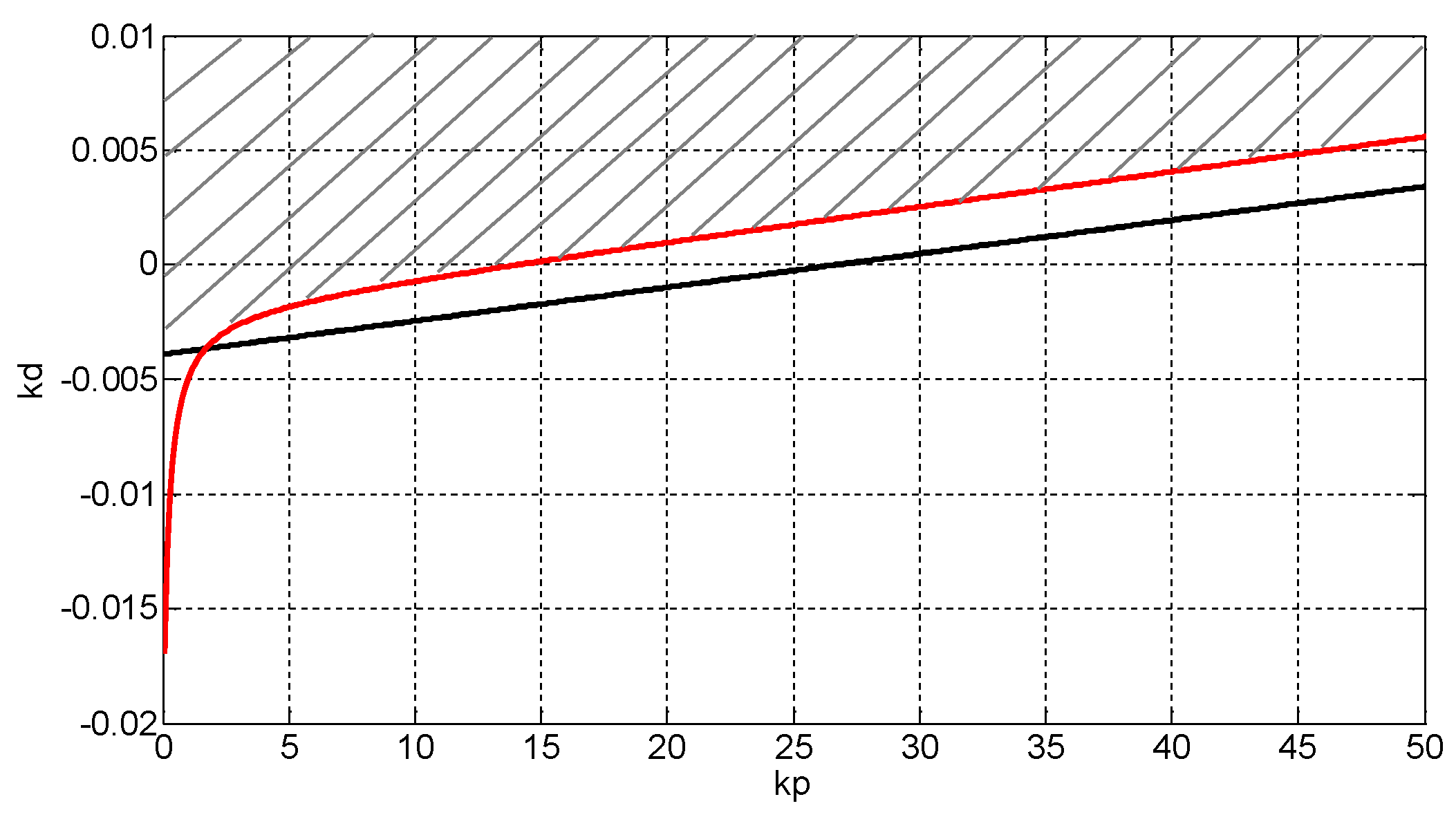
Since the function of PWM is to modulate a voltage signal which is the same as the reference voltage, the equivalent voltage gain satisfies . By solving the inequalities group (29) with the ignorance of the high order minor terms, parameter constraints for stability can be obtained as:
The shadow area shown in Figure 13 is the parameters constraint condition of stability. In addition, in order to achieve zero-axis signal tracking, the frequency selection and disturbance rejection performance of the control system at the low frequency should be taken into consideration.
Equation (22) shows that the system has conjugate poles at a specific frequency (fundamental frequency). By adjusting the control parameters and , the gain at the resonant frequency can be large enough to ensure zero steady-state error. Furthermore the additional open-loop zeros of PD controller can adjust the system bandwidth and high-frequency partial attenuation.
Therefore, the controller parameters constraint conditions can be described as: (1) In the parameters stability domain, the gain of the open loop system at the fundamental frequency is large. (2) Appropriate bandwidth of the closed-loop system is needed to ensure the response speed and the ability to suppress high-frequency interference.
Assume that the closed loop bandwidth frequency is , according to (25) and (28), the constraint conditions can be expressed as:
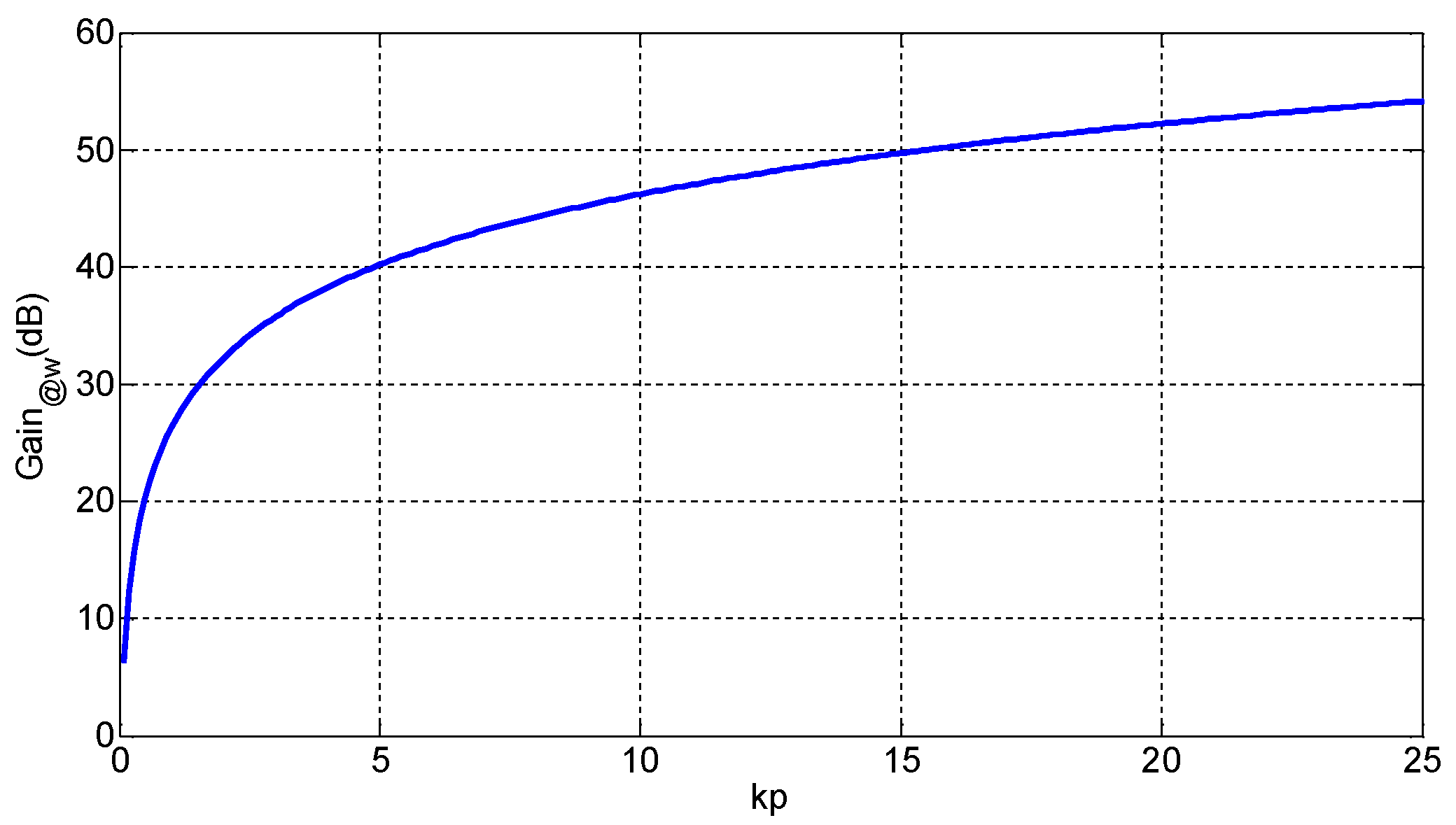
Equation (31) shows that the peak value of the open-loop resonant point at the fundamental frequency is only dependent on the coefficient , which is irrelevant to the differential coefficient . It means that the system steady-state error at the fundamental frequency is directly determined by the proportional coefficient. Considering the steady-state error and interference rejection for frequency fluctuation, the logarithmic gain range is selected as 40 dB~50 dB, which means the gain is greater than 100. The numerical relationship is shown in Figure 14. From the figure, the range of parameter can be chosen as .
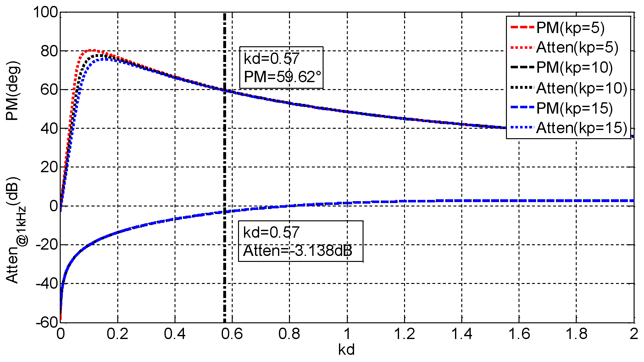
The differential coefficient is the molecular polynomial gain term of the open loop transfer function. So the system gain at the low frequency, the open loop and the closed loop bandwidth, and the phase margin are mainly determined by . Choose the switching frequency as 10 kHz, and the system bandwidth as 1/10 of switching frequency. Setting the , the attenuation of closed loop system at 1 kHz and phase margin of the open loop system are shown in Figure 15.
According to the system requirements of response speed and stability margin, the differential coefficient can be selected as . The corresponding phase margin of the closed-loop system is 59.62°, which represents high system stability. Selecting the system parameters as and , the open loop and closed loop characteristics of the zero-axis control system are shown in Figure 16.
The control system proposed in this paper is compared with the traditional system, as shown in Figure 17. The small graph in the figure is the partial enlarged detail at the fundamental frequency. When the system control parameters are similar (the system bandwidth is the same), two methods have little difference in the frequency characteristics in mid- and high-frequency areas. However,in the fundamental frequency band, the method proposed in this paper has a higher gain and a smaller phase shift. In another word, a small steady-state error is realized without the system dynamic characteristics changed.
5. Simulations and Experiments
5.1. Simulation and Experimental Conditions
In this paper, the Matlab/Simulink simulation software is used to simulate the three-phase four-leg inverter based on the zero-axis virtual coordinate system. Meanwhile, in order to verify the feasibility of the proposed algorithm, a three-phase four-leg inverter 30 kW prototype is built, and the algorithm experiment is carried out.
The topological structure of the inverter is shown in Figure 1. Three single-phase resistances are selected as load. Then the power imbalance can be created by switching resistance. The control scheme is designed in Figure 18. DC voltage outer loop and inductance current inner loop control are adopted as the control algorithm. In simulation, controller is sampled at fs = 10 kHz (100 μs) to mimic the operation inside a DSP, while the rest of the system, including inverter, filter, etc., are sampled at a higher rate to mimic the behavior of a inverter in real time (at least greater than 100 fs).
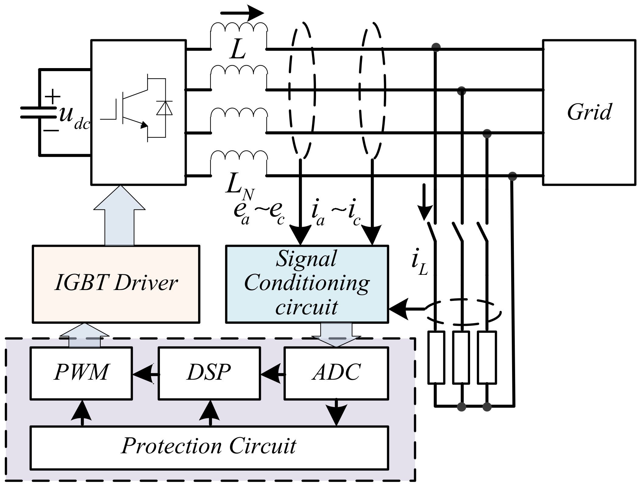
A structure diagram of the experimental system is presented in Figure 19. The Controller chip of the prototype is TMS320F28335 (Texas Instruments, Inc., Dallas, TX, USA). And the IGBT module is SKM150GB12V (Semikron, Ltd., Nuremberg, Germany), with the switching frequency of 10 kHz.
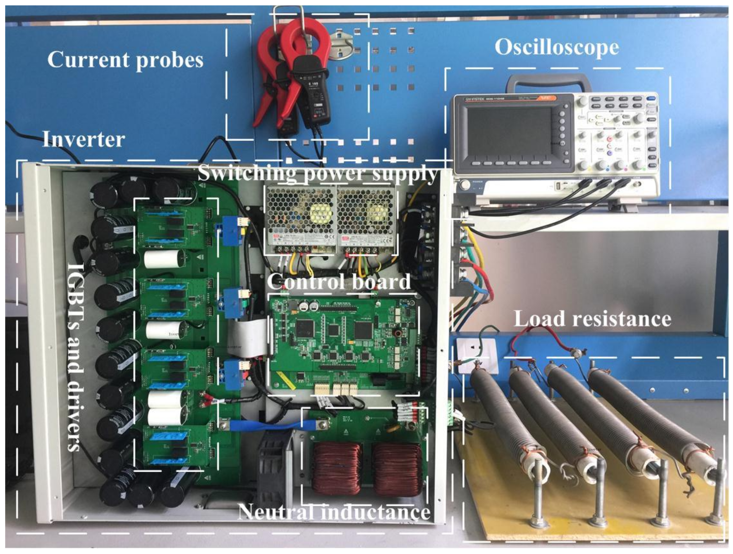
A photograph of the test rig is shown in Figure 20. The three-phase inductances of SPC are on the next layer and are not shown in the figure.
Table 1 lists the system parameters.
5.2. Steady State Analysis of System
With zero-sequence component considered only, a virtual three-phase zero-sequence reference current is set. Define the RMS of reference currents as , with the same phase as the A-phase voltage. Adopting the proposed zero-sequence control algorithm, the output current of the SPC is shown in Figure 21. The device current can track the reference current effectively. The three-phase current approximately coincides, with the same RMS of 18.3 A.
Figure 22 shows the simulation waveform of load current and inverter output current under unbalanced three-phase load. The load is set to an unbalanced extreme case: , and . It can be seen from the figure that the load is asymmetrical, and the output current is asymmetrical. The RMS values of the three-phase current are , , respectively, as shown in Figure 22a. After the extraction of the negative- and zero-sequence signal, the SPC device outputs the compensation current. The grid side current after compensation is shown in Figure 22b. The RMS values of the three-phase current are all 19.8 A. The zero line current RMS value is 0.1 A, indicating a high steady-state compensation precision.
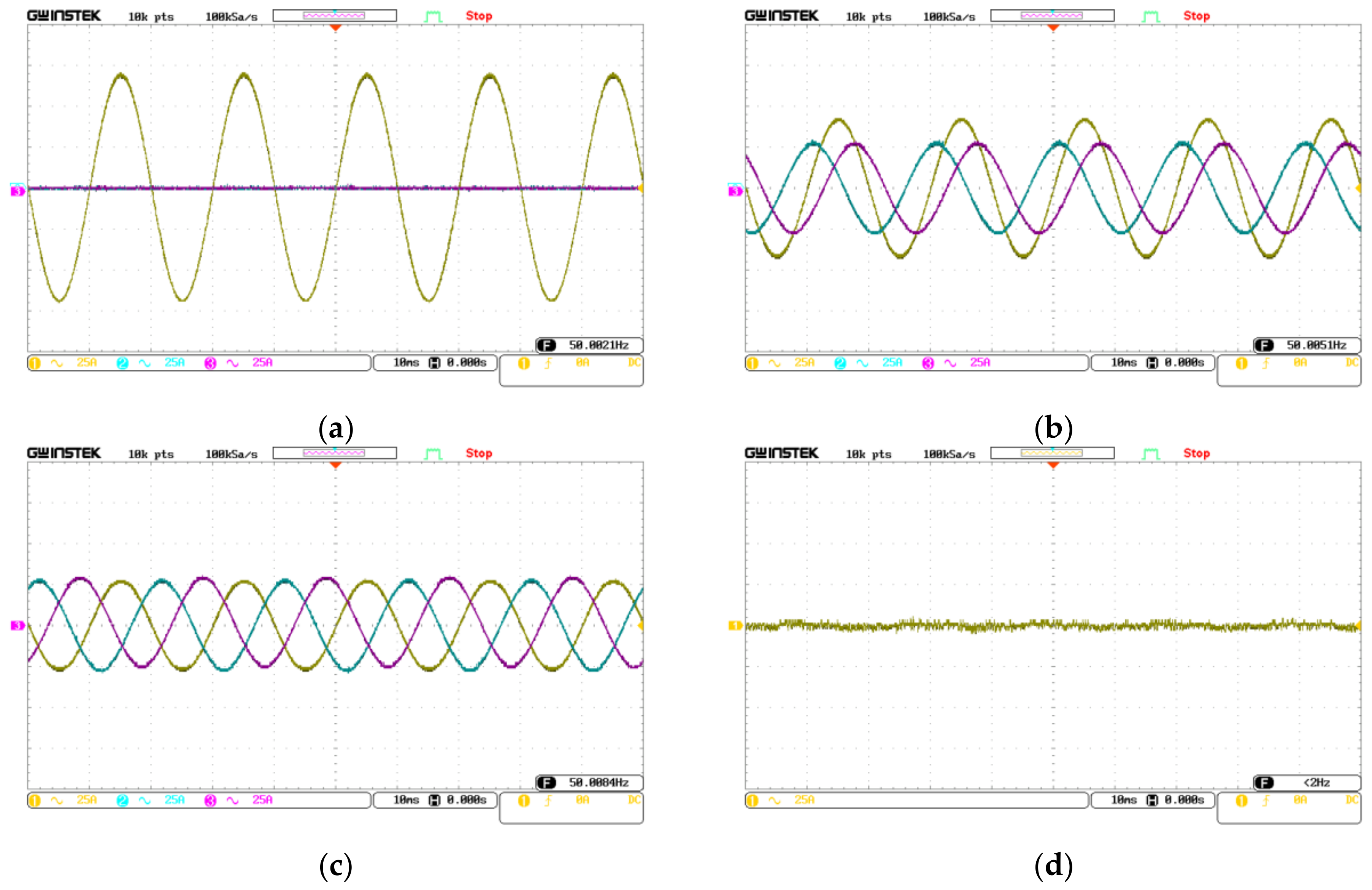
A GDS1104B oscilloscope (GWInstek, Ltd., Taiwan, China) is used as the experimental measuring instrument. Figure 23 shows the experimental waveform of unbalanced compensation with the single-phase resistor load. Figure 23a,c are the experimental waveforms of the grid side current before and after compensation. It can be seen that the single phase current is 50.3 A before compensation, and the three-phase grid current after compensation is 18.1, 17.7 and 17.9 A, respectively. The increase of current is caused by the loss of active power of compensation device. Figure 23d presents that the effective value of the zero line current after compensation is 1.2 A, the main component of which is the switch ripple. It shows that the zero-sequence fundamental current on the zero-axis is basically compensated.
5.3. Dynamic Analysis of System
In the initial case, , B-phase and C-phase are no-load. At 0.3 s, a resistive load is input to B-phase, tuning the load from an unbalanced state to another. At 0.8 s, B-phase load is removed and restored to the initial load state. The dynamic changes of the load and the system are shown in Figure 24.
Obviously, under the circumstances of sudden load increase or drop, unbalanced current can be quickly compensated. A fundamental period after the load fluctuate, the negative- and zero-sequence current are fully compensated. The response speed is fast, and the system enters the steady state again.
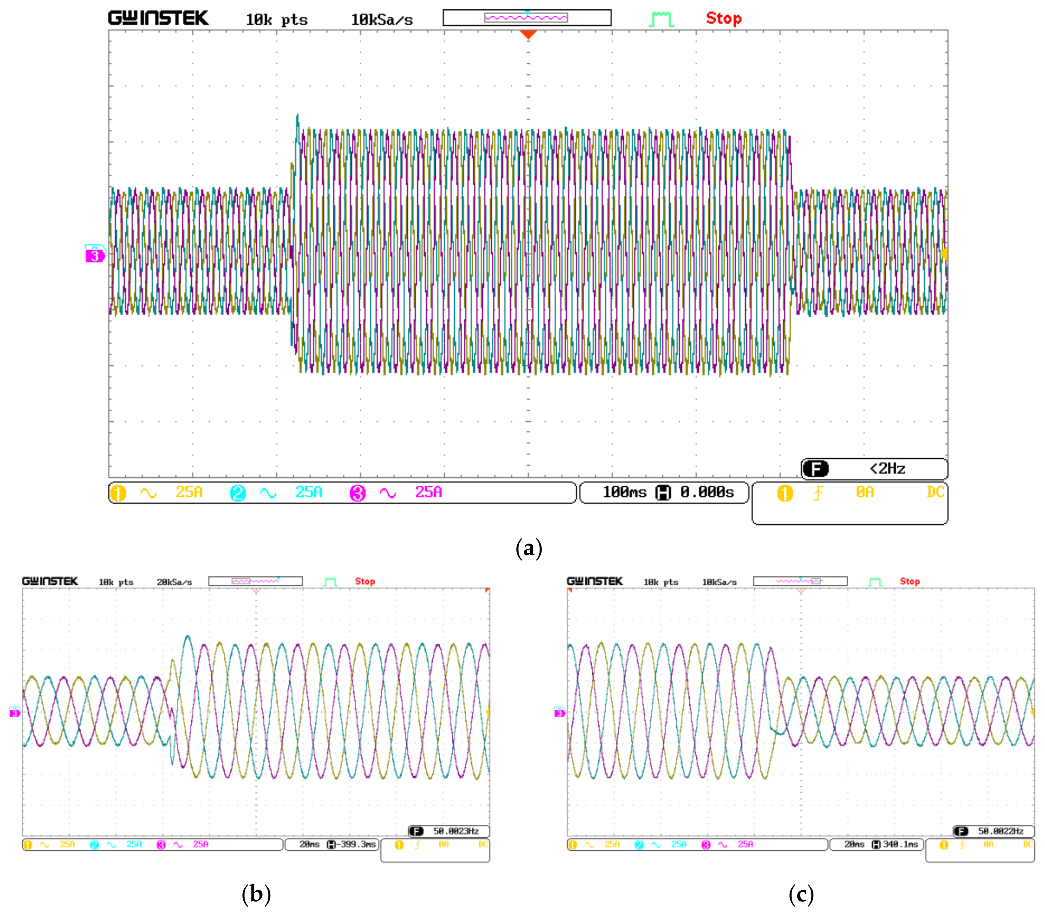
The load fluctuation experiment is carried out by using the prototype. And the experimental condition is similar to the simulation conditions. The experimental waveforms are shown in Figure 25. The experimental results show that when the load changes, the system responds quickly and realizes a complete compensation within a fundamental cycle.
6. Conclusions
In this paper, a new zero-axis current reconfiguration control algorithm is proposed to solve the problem of zero-axis current signal tracking for a three-phase four-leg static power compensator. First-order filters matrixes are constructed based on the linear transformation relation of positive-, negative- and zero-sequence signals. On the basis of matrices transformation and state feedback, the filters transmission matrixes-based orthogonal signal generator is proposed to achieve orthogonal signal generation and band-pass frequency selection. Next a zero-axis virtual synchronous coordinate system is established through mapping reconstruction. Then the controller is designed by adopting the pole zero placement method. In addition, the working characteristics of the proposed zero-axis control system are analyzed, and the controller parameters are designed. Compared with the traditional zero-axis direct control, this control strategy is equivalent to adding frequency tuning module by the orthogonal signal generator. The control gain of the open loop system can be effectively promoted through linear transformation. Finally, the theoretical evaluations are verified through simulation and experimental studies. The proposed zero-sequence current control algorithm has a good current control effect.
Author Contributions
L.Y. wrote the paper and designed the control method; C.F. contributed to the conception of the study and designed the simulation model; Y.Z. analyzed the system and participated in the design of prototype; J.L. helped to perform the analysis with constructive discussions.
Funding
This research was funded by [National Natural Science Foundation of China] grant number [51607179] and [Fundamental Research Funds for the Central Universities] grant number [2017QNB01].
Acknowledgments
This work is supported by the National Natural Science Foundation of China (Grant No. 51607179) and the Fundamental Research Funds for the Central Universities (2017QNB01).
Conflicts of Interest
The authors declare no conflict of interest.
Appendix A
Since , there is . When input sudden change occurs, the time domain attenuation rates of G0α(s) and G0β(s) are different. The mathematical expressions of i0α and i0β can be expressed as:
where , , , and are functions of I, , . Transformed to the sync virtual coordinate system, the current can be obtained as:
References
- Kong, W.; Ma, K.; Wu, Q. Three Phase Power Imbalance Decomposition into Systematic Imbalance and Random Imbalance. IEEE Trans. Power Syst. 2017, 33, 3001–3012. [Google Scholar] [CrossRef]
- Yan, S.; Tan, S.C.; Lee, C.K.; Chaudhuri, B.; Hui, S.Y.R. Electric Springs for Reducing Power Imbalance in Three-Phase Power Systems. IEEE Trans. Power Electron. 2015, 30, 3601–3609. [Google Scholar] [CrossRef] [Green Version]
- Hamajima, T.; Hu, N.; Ozcivan, N.; Soeda, S.; Yagai, T.; Tsuda, M. Balanced Three-Phase Distributions of Tri-Axial Cable for Transmission Line. IEEE Trans. Appl. Supercon. 2009, 19, 1748–1751. [Google Scholar] [CrossRef]
- Moses, P.S.; Masoum, M.A.S. Three-phase asymmetric transformer aging considering voltage-current harmonic interactions, unbalanced nonlinear loading, magnetic couplings, and hysteresis. IEEE Trans. Energy Conver. 2012, 27, 318–327. [Google Scholar] [CrossRef]
- Yousefi, B.; Soleymani, S.; Mozafari, B.; Gholamian, S.A.; Sciubba, E. Speed control of matrix converter-fed five-phase permanent magnet synchronous motors under unbalanced voltages. Energies 2017, 10, 1509. [Google Scholar] [CrossRef]
- Lopez, J.V.; Rodriguez, J.C.C.; Fernandez, S.M.; Garcia, S.M.; Garcia, M.A.P. Synthesis of fast onload multitap-changing clamped-hard-switching ac stabilizers. IEEE Trans. Power Deliv. 2006, 21, 862–872. [Google Scholar] [CrossRef]
- Gonzalez, D.; Hopfeld, M.; Berger, F.; Schaaf, P. Investigation on contact resistance behavior of switching contacts using a newly developed model switch. IEEE Trans. Compon. Packag. Manuf. Technol. 2018, 1–11. [Google Scholar] [CrossRef]
- Shateri, H.; Jamali, S. Measured impedance by distance relay for inter phase faults in presence of resistive Fault Current Limiter. In Proceedings of the IEEE International Conference on Power System Technology, Hangzhou, China, 24–28 October 2010. [Google Scholar] [CrossRef]
- Rawat, N.; Bhatt, A.; Aswal, P. A review on optimal location of FACTS devices in AC transmission system. In Proceedings of the IEEE International Conference on Power, Energy and Control, Sri Rangalatchum Dindigul, India, 6–8 February 2013. [Google Scholar] [CrossRef]
- Mangaraj, M.; Panda, A.K. NBP-based icosφ control strategy for DSTATCOM. IET Power Electron. 2017, 10, 1617–1625. [Google Scholar] [CrossRef]
- Fujun, M.; An, L.; Qiaopo, X.; Zhixing, H. Derivation of zero-sequence circulating current and the compensation of delta-connected static var generators for unbalanced load. IET Power Electron. 2016, 9, 576–588. [Google Scholar] [CrossRef]
- Kim, S.; Park, S.Y.; Kwak, S. Simplified model predictive control method for three-phase four-leg voltage source inverters. J. Power Electron. 2016, 16, 2231–2242. [Google Scholar] [CrossRef]
- Yaramasu, V.; Rodriguez, J.; Wu, B.; Rivera, M.; Wilson, A.; Rojas, C. A simple and effective solution for superior performance in two-level four-leg voltage source inverters: Predictive voltage control. In Proceedings of the IEEE International Symposium on Industrial Electronics, Bari, Italy, 4–7 July 2010; pp. 3127–3132. [Google Scholar] [CrossRef]
- Abronzini, U.; Attaianese, C.; D’Arpino, M.; Monaco, M.D.; Tomasso, G. Steady-state dead-time compensation in VSI. IEEE Trans. Ind. Electron. 2016, 63, 5858–5866. [Google Scholar] [CrossRef]
- Yepes, A.G.; Vidal, A.; López, O.; Doval-Gandoy, J. Evaluation of techniques for cross-coupling decoupling between orthogonal axes in double synchronous reference frame current control. IEEE Trans. Ind. Electron. 2014, 61, 3527–3531. [Google Scholar] [CrossRef]
- Dian, R.; Xu, W.; Mu, C. Improved negative sequence current detection and control strategy for h-bridge three-level active power filter. IEEE Trans. Appl. Supercond. 2016, 26, 1–5. [Google Scholar] [CrossRef]
- Perez-Estevez, D.; Doval-Gandoy, J.; Yepes, A.G.; Lopez, O.; Baneira, F. Enhanced resonant current controller for grid-connected converters with lcl filter. IEEE Trans. Power Electron. 2018, 33, 3765–3778. [Google Scholar] [CrossRef]
- Nian, H.; Shen, Y.; Yang, H.; Quan, Y. Flexible grid connection technique of voltage-source inverter under unbalanced grid conditions based on direct power control. IEEE Trans. Ind. Appl. 2015, 51, 4041–4050. [Google Scholar] [CrossRef]
- Kuperman, A. Proportional-resonant current controllers design based on desired transient performance. IEEE Trans. Power Electron. 2015, 30, 5341–5345. [Google Scholar] [CrossRef]
- Marati, N.; Prasad, D. A modified feedback scheme suitable for repetitive control of inverter with non-linear load. IEEE Trans. Power Electron. 2018, 33, 2588–2600. [Google Scholar] [CrossRef]
- Zhao, Q.; Ye, Y. A pimr-type repetitive control for a grid-tied inverter: Structure, analysis, and design. IEEE Trans. Power Electron. 2018, 33, 2730–2739. [Google Scholar] [CrossRef]
- Bayhan, S.; Abu-Rub, H.; Balog, R.S. Model predictive control of quasi-z-source four-leg inverter. IEEE Trans. Ind. Electron. 2016, 63, 4506–4516. [Google Scholar] [CrossRef]
- Pichan, M.; Rastegar, H.; Monfared, M. Deadbeat control of the stand-alone four-leg inverter considering the effect of the neutral line inductor. IEEE Trans. Ind. Electron. 2017, 64, 2592–2601. [Google Scholar] [CrossRef]
- Pichan, M.; Rastegar, H. Sliding mode control of four-leg inverter with fixed switching frequency for uninterruptible power supply applications. IEEE Trans. Ind. Electron. 2017, 64, 6805–6814. [Google Scholar] [CrossRef]
- Hamidi, A.; Ahmadi, A.; Feali, M.S.; Karimi, S. Implementation of digital fcs-mp controller for a three-phase inverter. Electr. Eng. 2015, 97, 25–34. [Google Scholar] [CrossRef]
- Yang, L.Y.; Wang, C.L.; Liu, J.H.; Jia, C.X. A novel phase locked loop for grid-connected converters under non-ideal grid conditions. J. Power Electron. 2015, 15, 216–226. [Google Scholar] [CrossRef]
- Wang, B.; San, G.; Guo, X.; Wu, W. Grid synchronization and PLL for distributed power generation systems. Proc. CSEE 2013, 33, 50–55. [Google Scholar]
Figure 1.
Schematic diagram of the SPC.

Figure 2.
Schematic diagram of the virtual rotating zero-axis coordinate system.
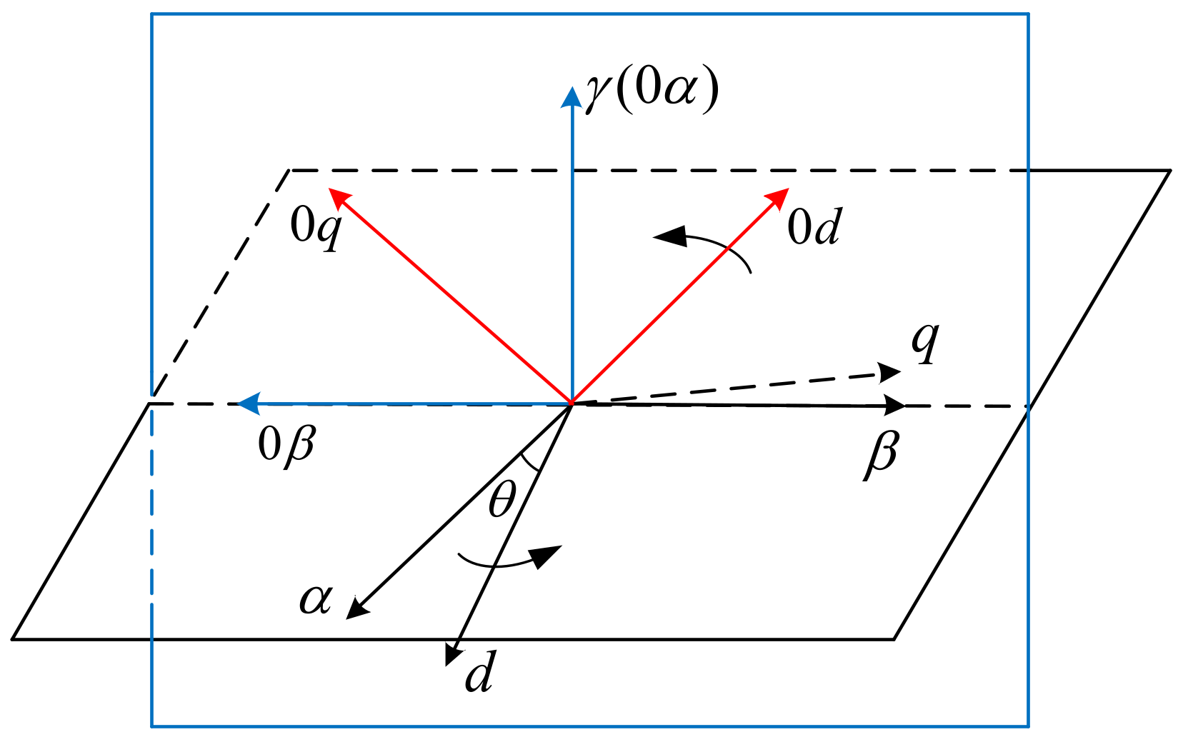
Figure 3.
Filter transmission matrixes signal processing module.
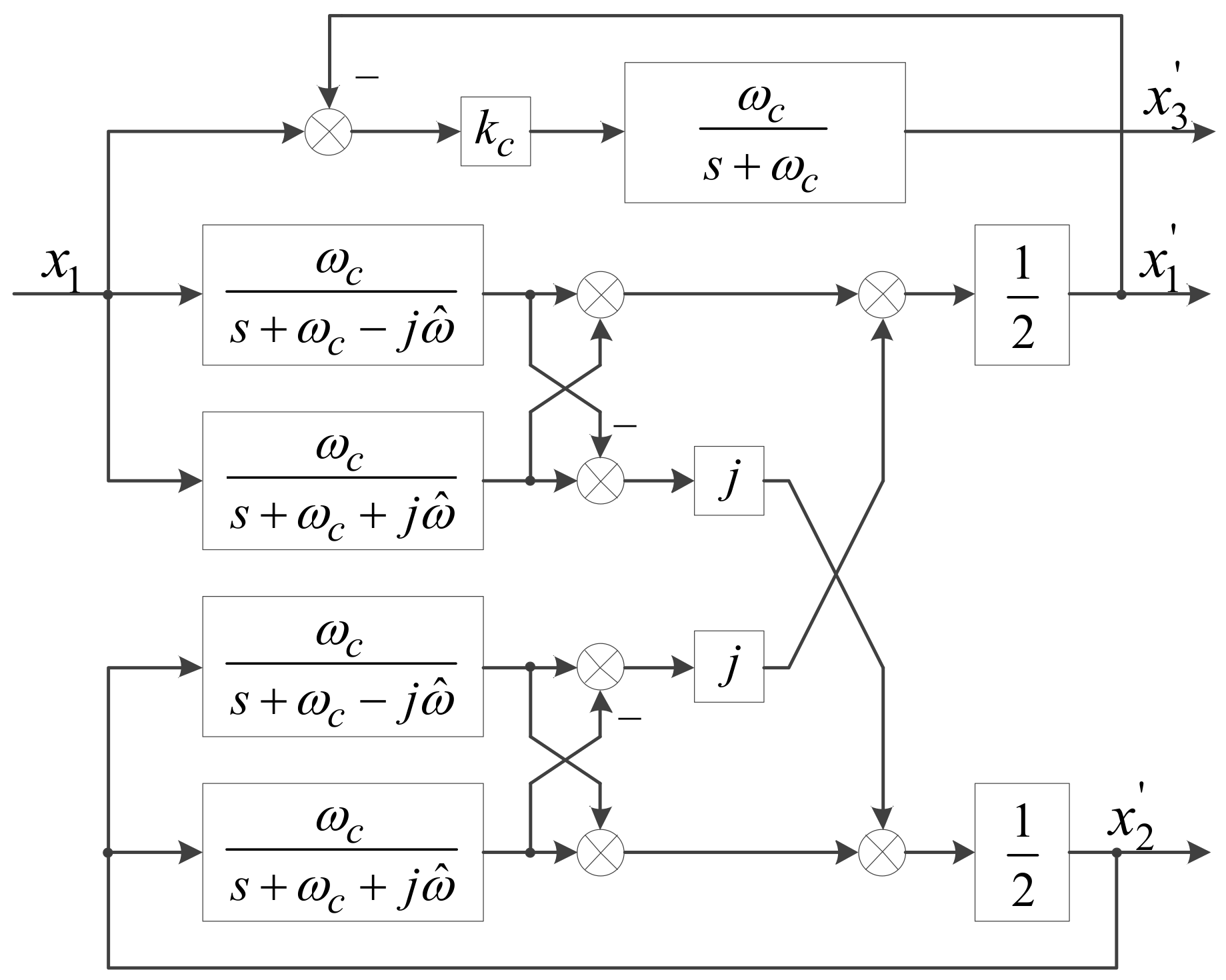
Figure 4.
Frequency characteristics of filter transmission matrixes signal processing module.

Figure 5.
Zero-axis current virtual mapping system.

Figure 6.
Zero-axis current control system diagram.
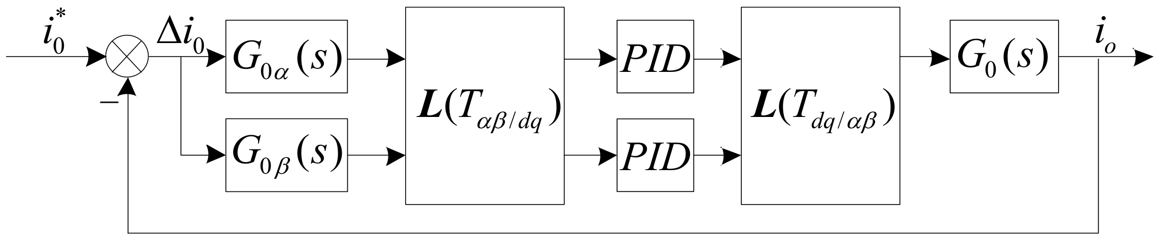
Figure 7.
Control block diagram of SPC.

Figure 8.
Quality factor change curve.
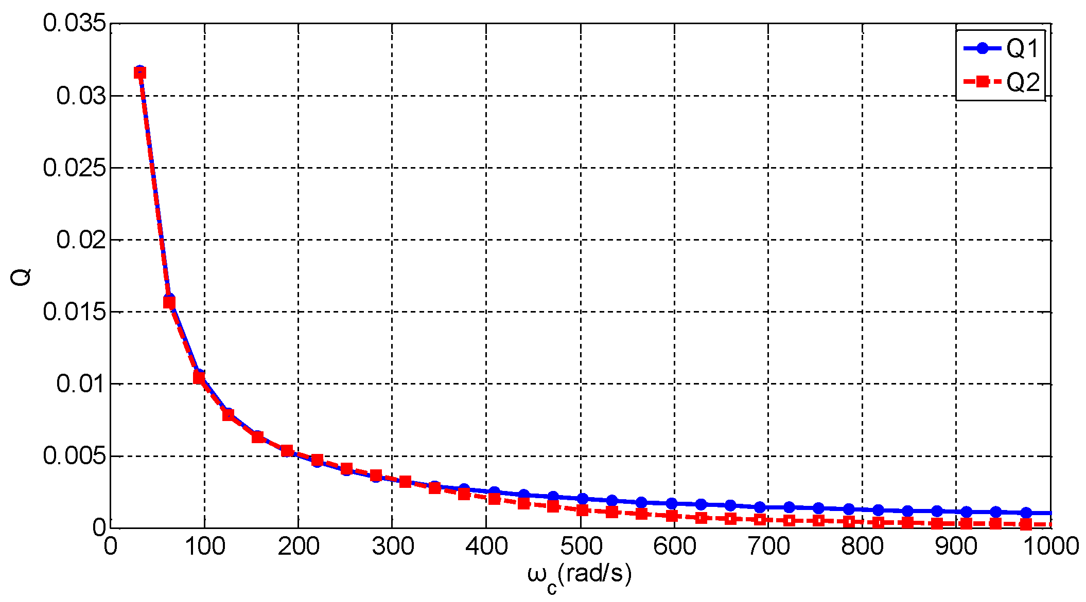
Figure 9.
Upper bound frequency and lower bound frequency variation curve.

Figure 10.
Characteristic roots locus.
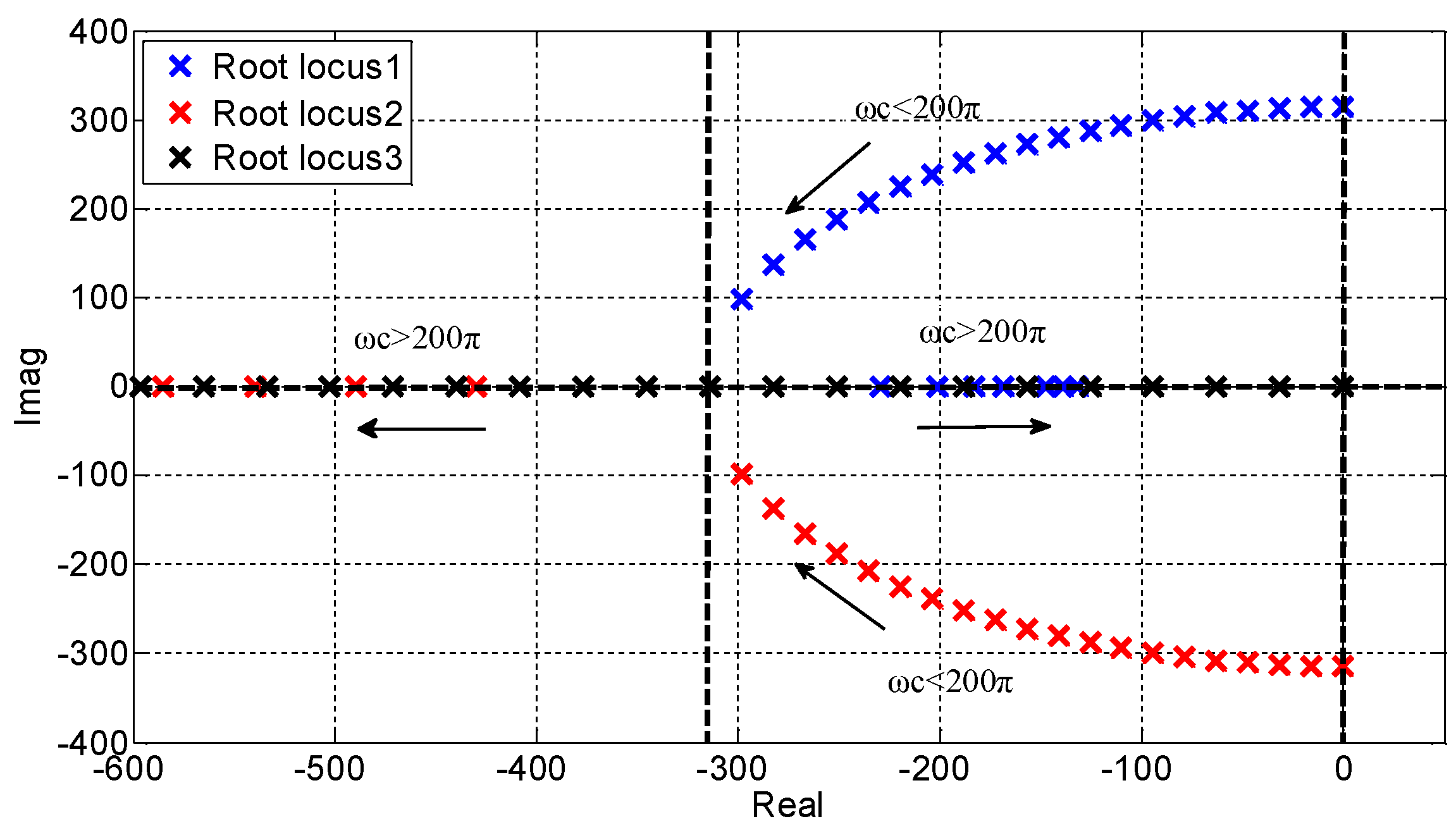
Figure 11.
Zero-axis current control block diagram.
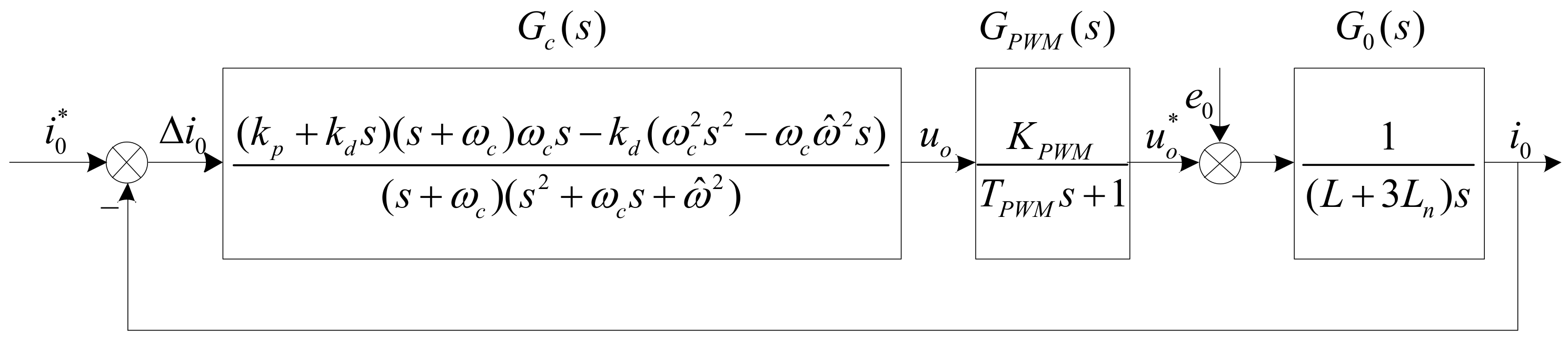
Figure 12.
Amplitude frequency characteristics of FTM-OSG.
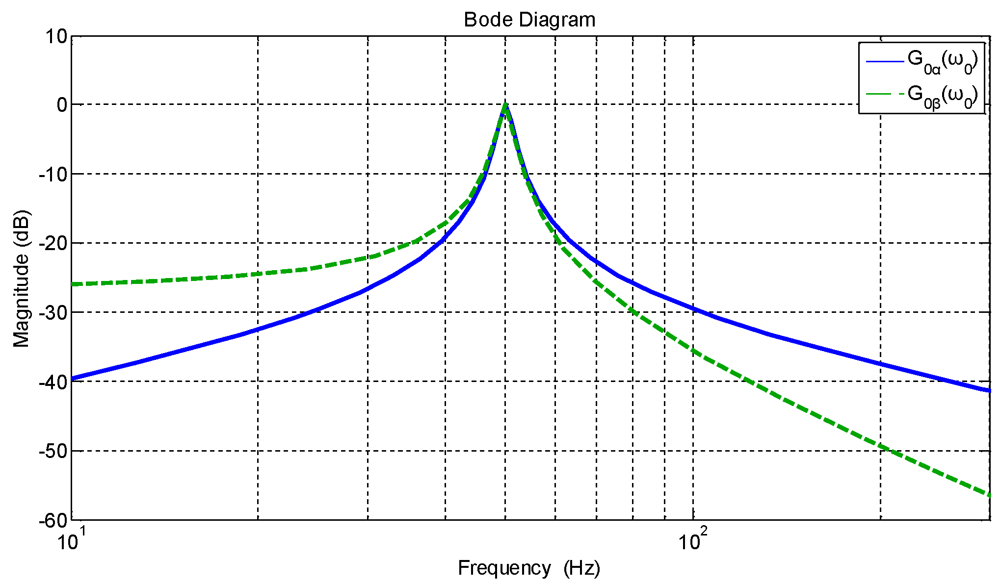
Figure 13.
Stability domain.

Figure 14.
The open loop transfer function gain curve based on kp.

Figure 15.
Relationship between kd and the frequency domain characteristics of system.

Figure 16.
Frequency domain characteristics curves of control system.
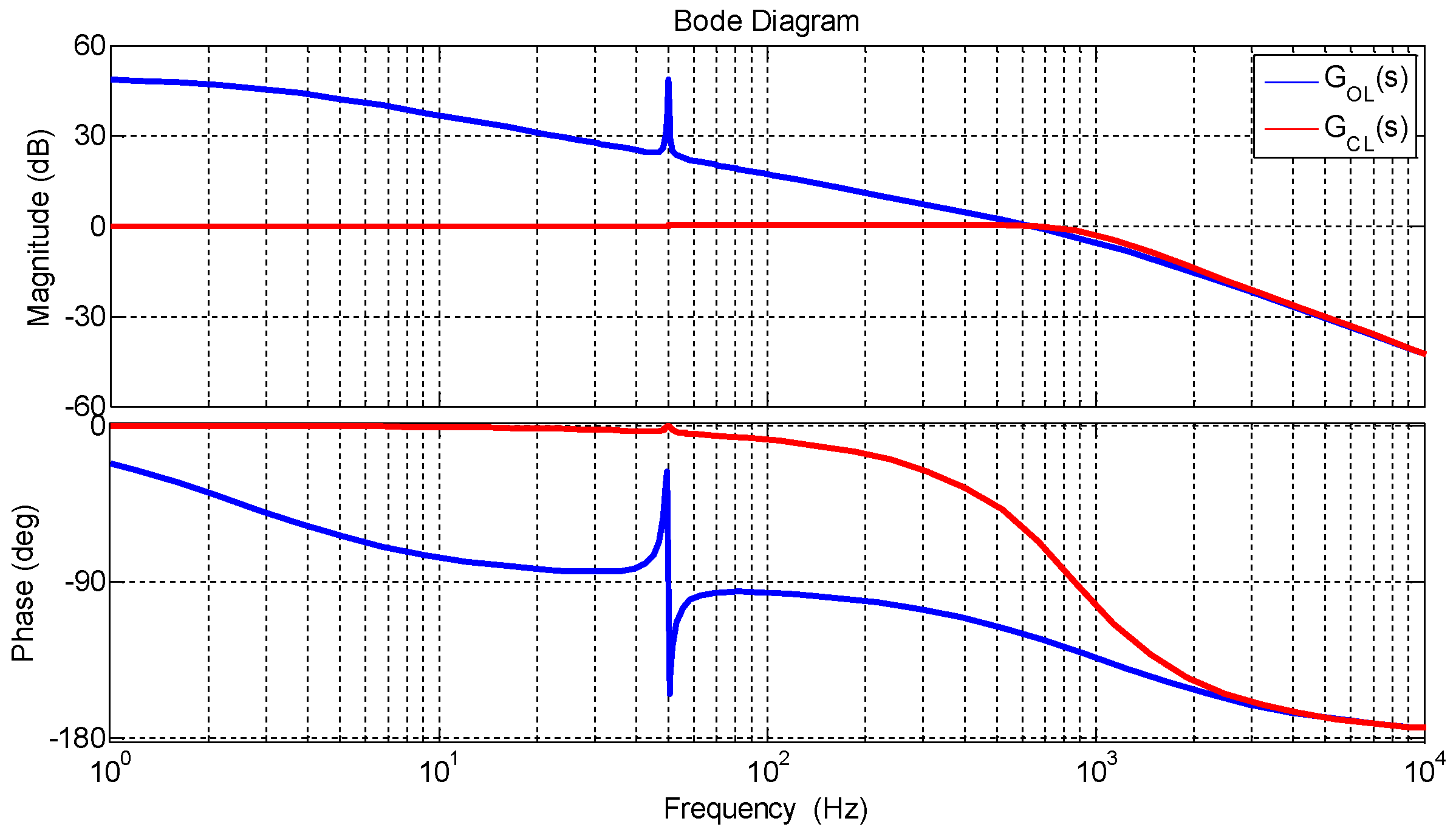
Figure 17.
Comparison of frequency domain characteristics of zero-axis control system.
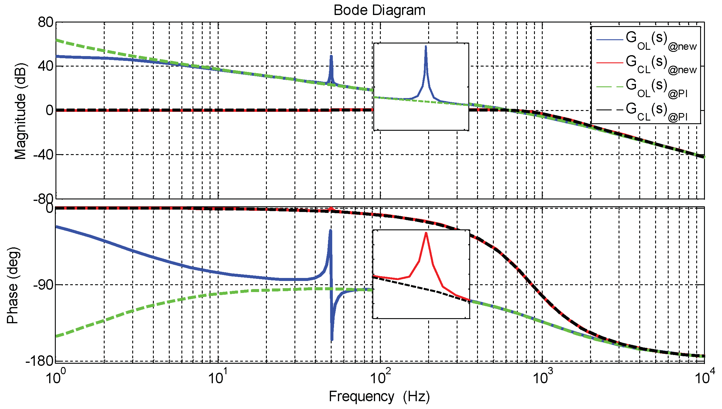
Figure 18.
System control scheme.

Figure 19.
Experimental system Structure diagram.

Figure 20.
Photograph of the experimental test rig.

Figure 21.
Zero-sequence current tracking waveform.

Figure 22.
Steady state simulation waveform of unbalanced load compensation: (a) Three-phase unbalanced load current; (b) The output current of the SPC device; (c) Grid current after compensation.
Figure 22.
Steady state simulation waveform of unbalanced load compensation: (a) Three-phase unbalanced load current; (b) The output current of the SPC device; (c) Grid current after compensation.
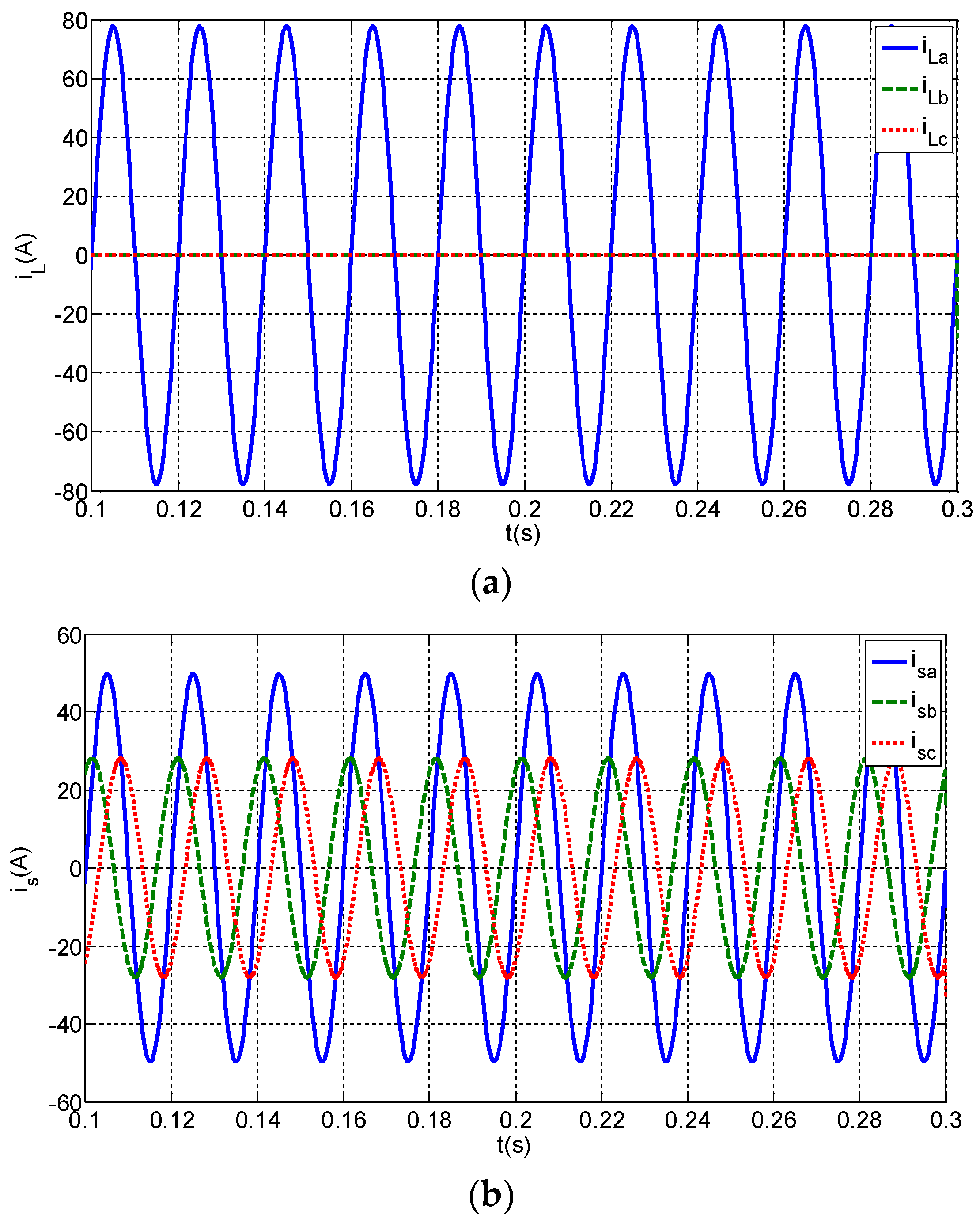
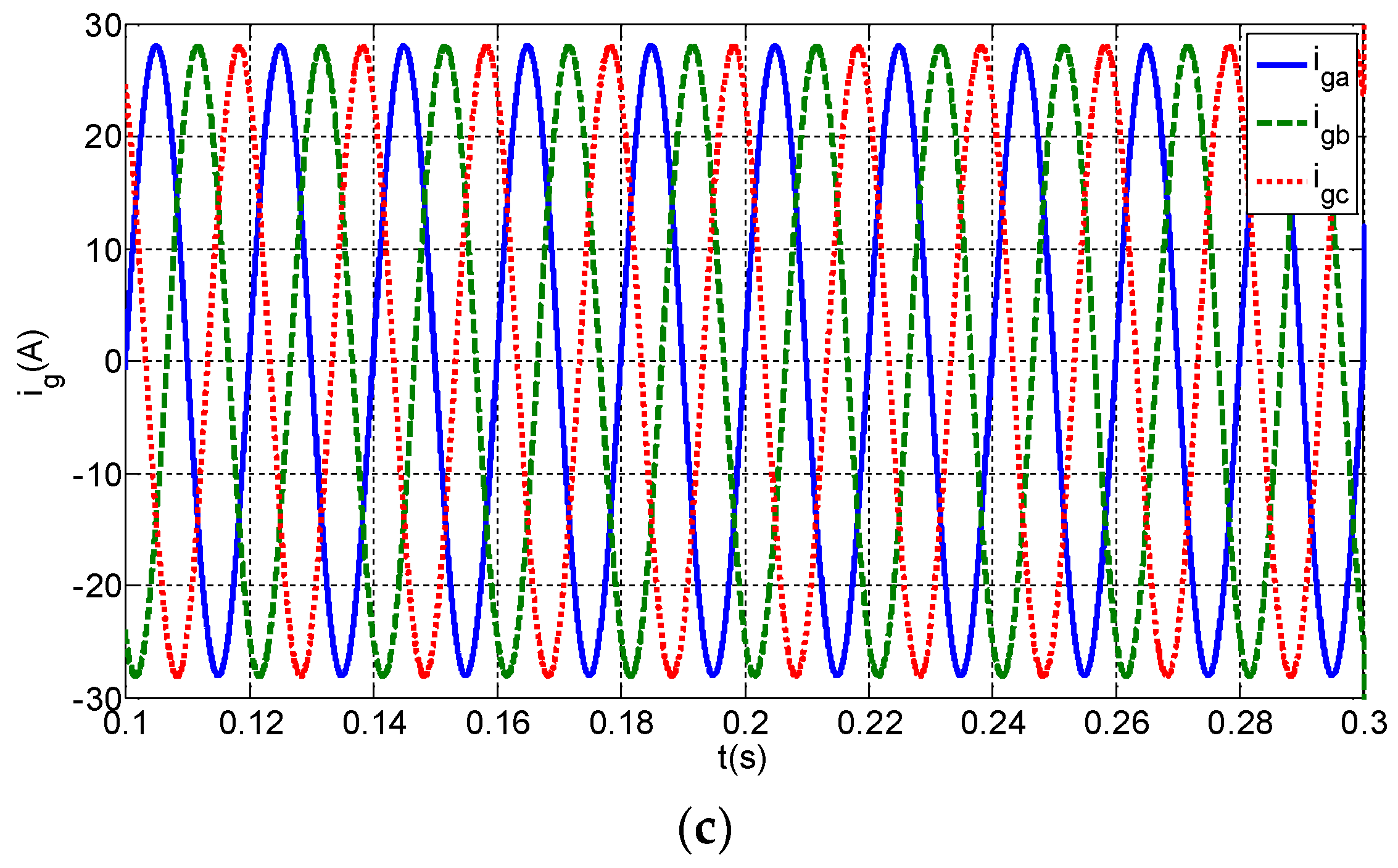
Figure 23.
Steady state experimental waveform of unbalanced load compensation: (a) Three-phase unbalanced load current; (b) Three-phase output current of SPC; (c) Three-phase grid current; (d) Zero line current.
Figure 23.
Steady state experimental waveform of unbalanced load compensation: (a) Three-phase unbalanced load current; (b) Three-phase output current of SPC; (c) Three-phase grid current; (d) Zero line current.

Figure 24.
Dynamic simulation waveform of unbalanced load compensation: (a) Three-phase unbalanced load current; (b) The output current of the SPC device; (c) Grid current after compensation; (d) RMS of grid current after compensation.
Figure 24.
Dynamic simulation waveform of unbalanced load compensation: (a) Three-phase unbalanced load current; (b) The output current of the SPC device; (c) Grid current after compensation; (d) RMS of grid current after compensation.
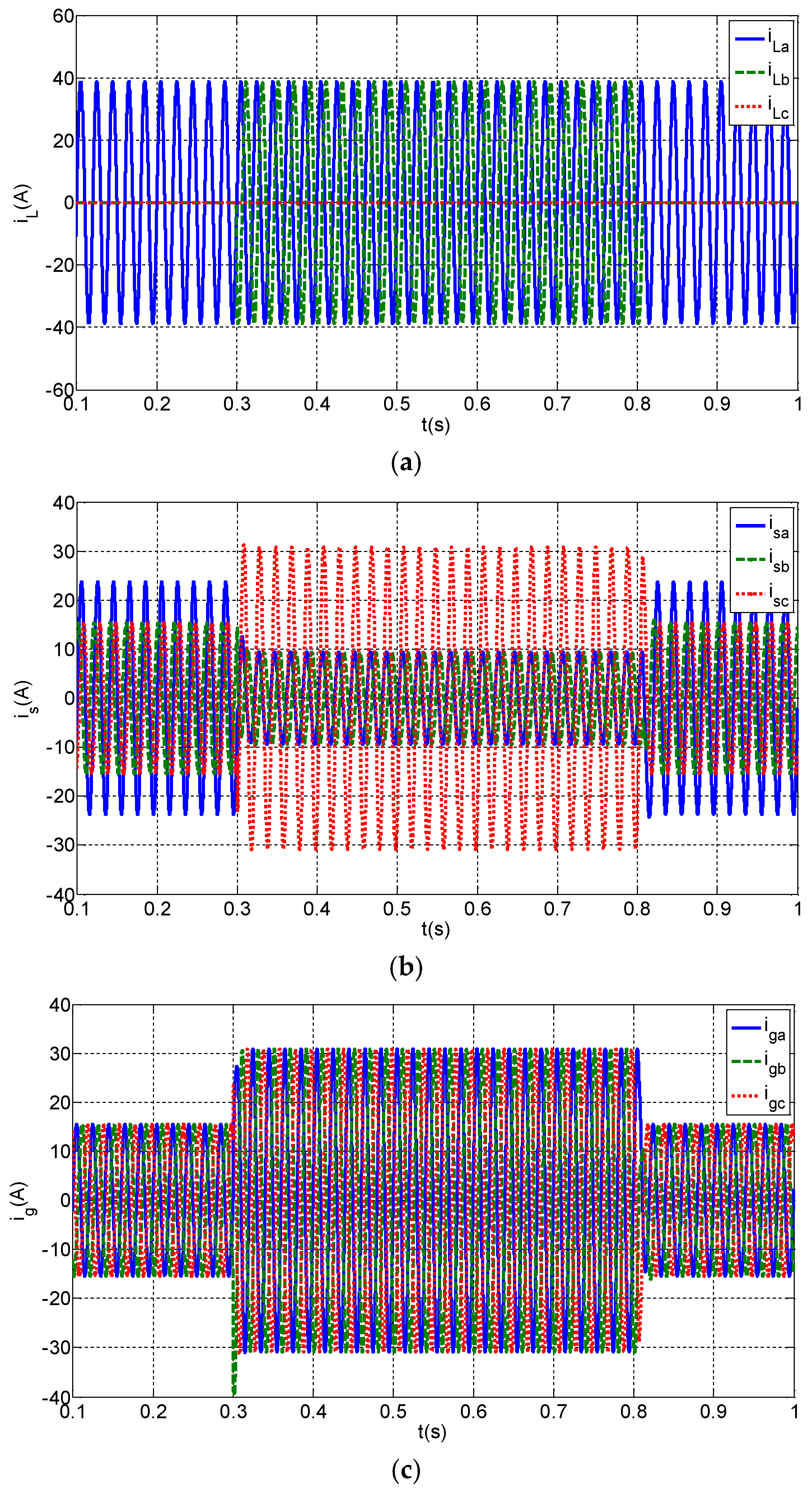
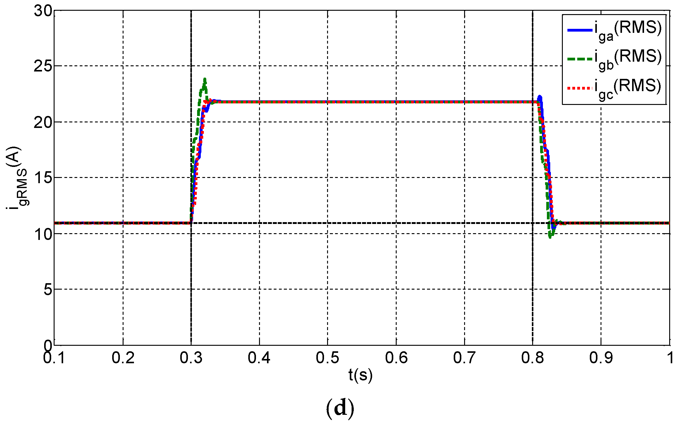
Figure 25.
Dynamic experimental waveform of unbalanced load compensation: (a) Three-phase grid current after compensation under load fluctuation; (b) Local enlargement of grid current with load increasing; (c) Local enlargement of grid current with load reducing.
Figure 25.
Dynamic experimental waveform of unbalanced load compensation: (a) Three-phase grid current after compensation under load fluctuation; (b) Local enlargement of grid current with load increasing; (c) Local enlargement of grid current with load reducing.

Table 1.
Parameters for the system.
| Parameter | Symbol | Value |
|---|---|---|
| Voltage (line voltage) | u | 380 V |
| Three-phase inductor | L | 0.5 mH |
| Zero line inductor | Ln | 0.5 mH |
| Switching frequency | f | 10 kHz |
© 2018 by the authors. Licensee MDPI, Basel, Switzerland. This article is an open access article distributed under the terms and conditions of the Creative Commons Attribution (CC BY) license (http://creativecommons.org/licenses/by/4.0/).
Share and Cite
MDPI and ACS Style
Yang, L.; Feng, C.; Zhao, Y.; Liu, J. Zero-Axis Virtual Synchronous Coordinate Based Current Control Strategy for Grid-Connected Inverter. Energies 2018, 11, 1225. https://doi.org/10.3390/en11051225
AMA Style
Yang L, Feng C, Zhao Y, Liu J. Zero-Axis Virtual Synchronous Coordinate Based Current Control Strategy for Grid-Connected Inverter. Energies. 2018; 11(5):1225. https://doi.org/10.3390/en11051225
Chicago/Turabian StyleYang, Longyue, Chunchun Feng, Yan Zhao, and Jianhua Liu. 2018. "Zero-Axis Virtual Synchronous Coordinate Based Current Control Strategy for Grid-Connected Inverter" Energies 11, no. 5: 1225. https://doi.org/10.3390/en11051225
Note that from the first issue of 2016, this journal uses article numbers instead of page numbers. See further details here.