Energy Management for Community Energy Network with CHP Based on Cooperative Game

Abstract

Integrated energy system (IES) has received increasing attention in micro grid due to the high energy efficiency and low emission of carbon dioxide. Based on the technology of combined heat and power (CHP), this paper develops a novel operation mechanism with community micro turbine and shared energy storage system (ESS) for energy management of prosumers. In the proposed framework, micro-grid operator (MGO) equipped with micro turbine and ESS provides energy selling business and ESS leasing business for prosumers. Prosumers can make energy trading with public grid and MGO, and ESS will be shared among prosumers when they pay for the rent to MGO. Based on such framework, we adopt a cooperative game for prosumers to determine optimal energy trading strategies from MGO and public grid for the next day. Concretely, a cooperative game model is formulated to search the optimal strategies aiming at minimizing the daily cost of coalition, and then a bilateral Shapley value (BSV) is proposed to solve the allocation problem of coalition’s cost among prosumers. To verify the effectiveness of proposed energy management framework, a practical example is conducted with a community energy network containing MGO and 10 residential buildings. Simulation results show that the proposed scheme is able to provide financial benefits to all prosumers, while providing peak load leveling for the grid.

1. Introduction

Due to the increasing concerns for environmental pollution and energy crisis, traditional power grid dominated by thermal power plant is facing serious challenges for low energy efficiency, high carbon emission, and increasing energy demand [1,2]. Based on such background, distributed generations, such as micro turbine generation and renewable energy generation, have already been applied widely in the grid [3]. Consequently, the concept of micro-grid emerges, which can operate as an independent system or as an energy demand side of public grid. In recent years, for the high energy efficiency, micro-grid has gradually developed into integrated energy system (IES), which can be expressed as a CHP (combined heating and power) system or CCHP (combined cooling, heating, and power) system [4,5,6,7,8]. In the IES, energy demand of end consumers is divided into multi-energy flows and such energy flows are provided separately by district transmission networks containing power wires, heating pipelines, and cooling pipelines (only exists for CCHP system). As a result, IES can make the energy efficiency reach to 70% or more, and can also reduce the carbon emission effectively. Moreover, in order to further improve the operation efficiency of micro-grid, except for distributed generations, energy management system (EMS) and energy storage system (ESS) are also the significant parts of micro-grid. EMS is responsible for the coordinated operation of the whole system, including the dispatching of generations’ energy output and scheduling of energy consumption in demand side [9]. Obviously, EMS is also the essential system in the implement of demand response (DR) project sponsored by public grid for peak shaving and valley filling of power load [10]. Furthermore, with the rapid cost reduction of advanced energy storage technologies, ESS is increasingly equipped in the micro-grid [11]. Since renewable energy generation is affected by environment (e.g., solar intensity, wind speed) seriously, ESS can be employed to store redundant produced energy during generation peak periods and provide energy in peak-demand hours, which will contribute the performance of IES and DR project.

In recent years, research works have been widely conducted from the perspective of modeling with different resources in the micro-grid. For the renewable energy generation (e.g., photovoltaic, wind), works are generally focused on the maximal consumption and uncertainty of energy output. The authors in [12] proposes a stochastic programming for the minimization of expected operational cost and power losses while accommodating the intermittent nature. Wei et al. [13] proposes an online optimal operation approach considering prediction error of renewable energy generation and load. For the ESS, there is more attention paid on the scheduling of charging/discharging strategy or the operation of ESS capacity. In [14], a method is presented for determining optimal size of ESS for primary frequency control of a Microgrid. When ESS is configured in demand side management, the strategy will be scheduled considering the price mechanism and shiftable load demand. Authors in [15] has discussed equilibrium problem among residential consumers in energy consumption scheduling based on game-theoretic approaches considering ESS selling back energy to grid. For the modeling of load, electrical loads of residential users are generally divided into basic load without DR potential and flexible load that can participate in the DR [16]. Literature [17] found the model for three kinds of flexible load from the physical properties of load’s energy consumption, including shiftable and interruptible load, shiftable but non-interruptible load, and interruptible but non-shiftable load. Authors in [18] analyze the Nash equilibrium with game-theoretic approach considering the participation of flexible load in DR under time-of use pricing. For the CHP/CCHP system based on micro turbine, the most important are the scheduling and dispatching of multi energy flow. Literature [19] proposes an optimization model for the short-term scheduling of IES’s energy flows, and then converts the founded nonlinear model with appropriate piecewise linear approximation. Authors in [20] takes operating costs, carbon dioxide emissions and energy efficiency as judgment standards of IES’s performance, and then study the influence on the performance of IES with different optimal strategies. While in [21], authors present a mixed-integer linear programming super-structure model for the optimal design of IES that satisfies the heating and power demand at the level of a small neighborhood. A game theoretic optimization method is introduced in literature [22], and authors puts forward a multi-energy management framework for IES based on the Stackelberg game, in which micro-grid is the leader and consumers are the followers. When CHP/CCHP system is configured with ESS, the existed researches intend to improve the system efficiency or satisfy the fluctuation of demand. Literature [23] provides a generic energy systems engineering framework toward the optimal design of IES in China under the existence of battery, thermal storage, and ice storage. Authors in [24] propose a scenario system in which a domestic engine-based CHP is integrated with a hybrid ESS containing batteries and super-capacitors, and experimental tests show that the system can satisfy the fluctuant energy demands in a domestic dwelling.

Based on the above referred research, by integrating distributed generations, ESS, EMS, and DR, a micro-grid can be expected to solve the problem of current power grid effectively under the circumstance of well-established operation mechanism. Accordingly, in this paper, via considering the integration of photovoltaic (PV) generation, micro turbine, shared ESS, EMS, and DR in the micro-grid, a novel operation mechanism is introduced for grid-connected IES based on residential community energy network. In our framework, micro-grid operator (MGO) is a profit organization who provides energy selling business with its micro turbine and energy storage business with its ESS; while traditional user is changed into prosumer who has dual identity as an energy consumer and an energy producer with PV generation. Prosumers can purchase energy from public grid or MGO, additionally, they can store surplus energy to MGO’s ESS and then withdraw it to make up energy deficit as long as prosumers pay for the rent to MGO. Considering cooperation can generally create cooperative surplus, for the low energy consumption cost, prosumers in the community are willing to participate in the cooperation and make energy trading with MGO or public grid as a coalition, and also willing to participate in the DR project. Although prosumers choose to participate in the coalition, the ultimate goal is still the minimization of self-cost. Hence, it is necessary to re-allocate the coalition cost into each prosumer fairly. Based on above analysis, this paper concentrates on the day-ahead energy scheduling and coalition cost allocation problem for prosumers with cooperative game. In brief, the contributions of this paper are as follows.

• A novel operation mechanism is proposed to schedule energy consumption and purchasing strategies for prosumers considering community energy network equips with micro turbine and shared ESS.
• A cooperative game approach is formulated for the proposed scenario to reduce the total cost of all prosumers, and then a distribution mechanism based on bilateral Shapley value (BSV) is employed to allocate the coalition cost.
• Community energy network which contains 10 residential buildings are conducted to validate the effectiveness and efficiency of the proposed approach.

The system model is introduced in Section 2. In Section 3, cooperative game among prosumers is formulated. Section 4 focuses on the distribution mechanism. Then, simulation results are presented in Section 5. Finally, this paper is concluded in Section 6.

2. System Model

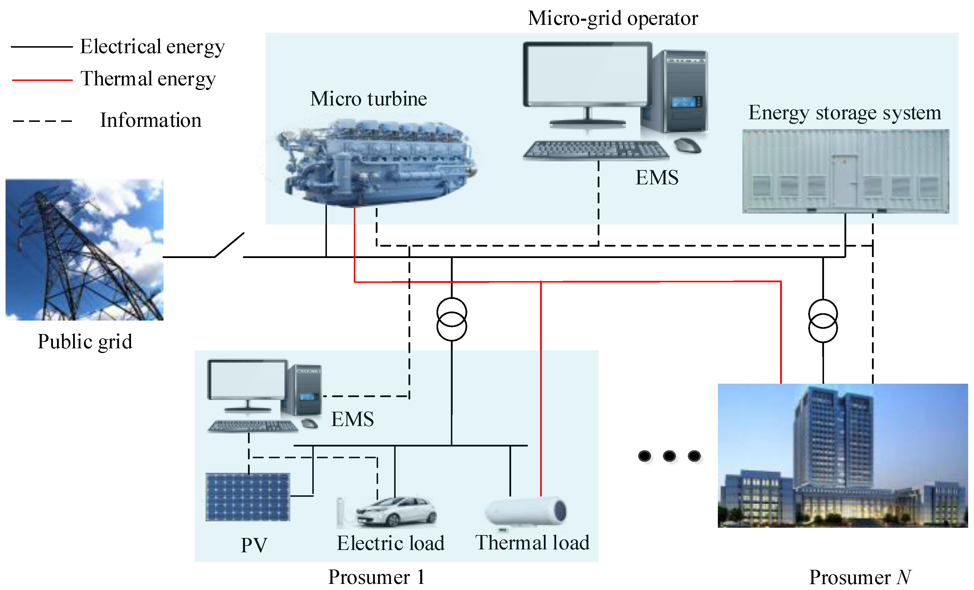
The structure of community energy network is shown in Figure 1. Community energy network is a micro integrated energy system which consists of MGO and multiple prosumers. MGO has micro turbine and ESS, who can sell electrical and thermal energy to prosumers, and meanwhile provide energy storage leasing business for prosumers. The scheduling and dispatching for turbine and energy storage are both executed by EMS of MGO. Each prosumer is equipped with EMS, PV generation, electrical load, thermal load. Note that, cooling load of each prosumer has been included in electrical load, and thermal load can obtain energy supply from micro thermal grid or power grid. Here, EMS of MGO is responsible by independent service department of MGO; while smart meter is in charge of the operation of prosumer’s EMS. In the proposed scenario, prosumer can store surplus energy to ESS but needs to pay lease expense to the MGO. When prosumers have a high energy demand, they will take back the stored energy from storage or purchase energy from MGO and public. Furthermore, DR is considered in the scenario by public grid setting an effective pricing mechanism. In order to conduct DR project perfectly, we assume that prosumer EMS can control and schedule energy consumption of partial electrical load, and prosumer EMS will communicate with EMS of MGO via information network.

Suppose that there are N prosumers in the whole community energy network with the set $\mathcal{N}=\left\{1,2,\cdots ,N\right\}$. Additionally, this paper is focused on the day-ahead energy scheduling, thus assume that a day is divided into T time slots with the set $\mathcal{T}=\left\{1,2,\cdots ,T\right\}$.

2.1. Model of Micro Turbine

Micro turbine, which can provide electricity and heat simultaneously, is an important equipment in the IES. The high-temperature heat (i.e., 900–1200 ${}^{\circ }$C) in the turbine is used to produce electricity, and then residual heat ( i.e., 100–500 ${}^{\circ }$C) will be recycled by heat recovery boiler for thermal demand of prosumers. We assume that natural gas is the energy source of turbine. Accordingly, the electricity and recycled heat output of micro turbine can be calculated as [25]

$$\left\{\begin{array}{c}{p}_g^{et}={\eta }_g^e{\lambda }_{gas}{\gamma }_g^{et}\\ p_g^{ht}={\eta }_g^h\left(1-{\eta }_g^e\right){\lambda }_{gas}{\gamma }_g^{et}\end{array}\right.$$

(1)

where $p_g^{et}$ is electricity output and $p_g^{ht}$ is recycled heat output in time slot t; ${\eta }_g^e$ is electricity generation efficiency of turbine; ${\eta }_g^h$ is recovery efficiency of residual heat; ${\gamma }_g^{et}$ is gas consumption rate; ${\lambda }_{gas}$ is calorific value of natural gas.

2.2. Energy Storage System

Shared ESS in the proposed scenario is provided by MGO for surplus energy storage of prosumers. In the ESS model, we assume that its maximal capacity is sufficient to support all prosumers’ transactions. Suppose that energy state of ESS is $Soc\left(t\right)$ in time slot t. Considering energy conversion losses in the operation, ESS charging and discharging efficiencies are represented by ${\eta }_{ch}$ and ${\eta }_{dis}$, respectively, where $0\le {\eta }_{ch},{\eta }_{dis}\le 1$. Moreover, an energy loss rate ${\eta }_{loss}$ is considered in the ESS model that results in reduction of stored energy with time. Accordingly, if energy state of ESS is $Soc\left(t-1\right)$ at the beginning of time t, then state of ESS $Soc\left(t\right)$ at the end of time t can be calculated as [26]

$$Soc\left(t\right)={\eta }_{loss}Soc\left(t-1\right)+{\eta }_{ch}\sum _{n=1}^N{p}_{ESS,n}^{ch,t}-1/{\eta }_{dis}\sum _{n=1}^N{p}_{ESS,n}^{dis,t}$$

(2)

where $p_{ESS,n}^{ch,t}$ and $p_{ESS,n}^{dis,t}$ are charging and discharging energy of prosumer n in time slot t, respectively. ${\eta }_{ch}{\displaystyle \sum _{n=1}^N}{p}_{ESS,n}^{ch,t}$ represents the actual energy charged in the ESS when all prosumers have ${\displaystyle \sum _{n=1}^N}{p}_{ESS,n}^{ch,t}$ amount of redundant energy; while ESS will discharge $1/{\eta }_{dis}{\displaystyle \sum _{n=1}^N}{p}_{ESS,n}^{dis,t}$ amount of energy when all prosumers withdraw ${\displaystyle \sum _{n=1}^N}{p}_{ESS,n}^{dis,t}$ amount.

2.3. Model of Prosumer’s Load

In the IES, load demand can be divided into different types (e.g., electrical, thermal, and cooling load) based on the load characteristic. Considering that cooling demand of users is mainly provided by air conditioner in recent years, cooling load of prosumers in the scenario is considered as electrical load. In addition, PV generation of prosumer can be considered as a special load which consumes negative energy.

(1) Electrical load

In this study, we assume that prosumers are willing to participate in the DR. That is, a certain percentage of electrical load will have the room for adjusting the consumption amount and time slot. Consequently, electrical load is divided into two types in our paper: basic load and shiftable load.

(a) Basic load

Basic load generally requires high reliable energy supply and static consumption time. Prosumers will be influenced seriously if such load is scheduled, such as lights, refrigerators, televisions. Basic load vector is defined as

$$l{e}_{bn}=\left[l{e}_{bn}^1,\dots ,l{e}_{bn}^t,\dots ,l{e}_{bn}^T\right]$$

(3)

where $l{e}_{bn}^t$ denotes the energy consumption of whole basic load at time t for prosumer n. In addition, the consumption model of basic load can be expressed as

$$\left\{\begin{array}{cc}l{e}_{bn}^{at}=0& t\notin \left[t_a^{on},t_a^{off}\right]\\ l{e}_{bn}^{at}=l{e}_{bn}^a& t\in \left[t_a^{on},t_a^{off}\right]\end{array}\right.$$

(4)

where $t_a^{on}$ and $t_a^{off}$ are start running time and end time, respectively; $l{e}_{bn}^a$ is the rated energy consumption of load a; $l{e}_{bn}^{at}$ is the energy consumption of basic load a at time t and satisfy

$$l{e}_{bn}^t=\sum _{a\in {\mathcal{A}}_{bn}}l{e}_{bn}^{at}$$

(5)

where ${\mathcal{A}}_{bn}$ is the set of basic load of prosumer n.

(b) Shiftable load

Different from basic load, shiftable load is relatively insensitive to energy consumption time and can be shifted in a certain time range interval, such as electric vehicle, washing machine, and dishwasher. Therefore, such load has contribution to DR which can be scheduled for the peak shaving or cost reduction. Shiftable load vector is defined as

$$l{e}_{sn}=\left[l{e}_{sn}^1,\dots ,l{e}_{sn}^t,\dots ,l{e}_{sn}^T\right]$$

(6)

where $l{e}_{sn}^t$ denotes the energy consumption of whole shiftable load at time t for prosumer n. In addition, the consumption model of shiftable load can be expressed as

$$\left\{\begin{array}{c}l{e}_{sn}^{at}=0\hfill \\ l{e}_{sn}^{at}\in \left[l{e}_{sn}^{a,min},l{e}_{sn}^{a,max}\right]\hfill \end{array}\right.\begin{array}{c}t\notin \left[t_a^{on},t_a^{off}\right]\\ t\in \left[t_a^{on},t_a^{off}\right]\end{array}$$

(7)

$$\left[t_a^{on},t_a^{off}\right]\in \left[{\alpha }_a,{\beta }_a\right]$$

(8)

$$\sum _{t={\alpha }_a}^{{\beta }_a}l{e}_{sn}^{at}=Q_a$$

(9)

where $l{e}_{bn}^{at}$ is the energy consumption of shiftable load a at time t; $l{e}_{sn}^{a,min}$ and $l{e}_{sn}^{a,max}$ are minimal and maximal energy consumption of load a; $\left[{\alpha }_a,{\beta }_a\right]$ is the optional time range interval of the of load a; $Q_a$ is the energy demand of load a in a whole day; $l{e}_{sn}^{at}$ is the energy consumption of load a at time t and satisfy

$$l{e}_{sn}^t=\sum _{a\in {\mathcal{A}}_{sn}}l{e}_{sn}^{at}$$

(10)

where ${\mathcal{A}}_{sn}$ is the set of shiftable load of prosumer n.

(2) Thermal load

In our proposed scenario, thermal demand of prosumer would be satisfied by purchasing heat from MGO or producing heat with household appliance. For example, hot water demand for bath can be provided uniformly from MGO via water pipeline, but prosumer can also use electric or gas water heater to satisfy the same demand. If prosumers equip with gas-based appliances, thermal load will be classified as gas load; if prosumers equip with electricity-based appliances, thermal load will be classified as basic electric load which satisfies Equation (4). Since this paper mainly considers the electricity energy management of prosumers, assume that all prosumers have equipped with electric appliance for thermal demand. Similarly, thermal load vector is defined as

$$l{h}_n=\left[l{h}_n^1,\dots ,l{h}_n^t,\dots ,l{h}_n^T\right]$$

(11)

where $l{h}_n^t$ denotes the energy consumption of whole thermal load at time t for prosumer n.

(3) PV generation

Energy output of PV generation is influenced by environment (e.g., solar intensity, temperature) and PV-self property (e.g., surface area, conversion efficiency, dirt on the surface) [27]. However, the main influence factors are solar intensity, surface area, and conversion efficiency. Therefore, an approximate model for PV output can be employed [28]:

$$p_{PV}={\eta }_{PV}{S}_{PV}I$$

(12)

where ${\eta }_{PV}$ is PV conversion efficiency; $S_{PV}$ is the surface area of PV panel ; I is the valid solar intensity absorbed by PV panel. In which, solar intensity I is influenced by weather condition (e.g., sunny day, rainy day, cloudy day) and installation of PV panel (e.g., tilt angle, azimuth angle); Surface area $S_{PV}$ is the valid area that can absorb the solar intensity. Accordingly, energy output vector of PV generation is defined as

$$p{v}_n=\left[p{v}_n^1,\dots ,p{v}_n^t,\dots ,p{v}_n^T\right]$$

(13)

where $p{v}_n^t$ denotes the energy output of PV generation at time t for prosumer n.

3. Game-Theoretic Optimization for Prosumers

To achieve a lower daily energy cost, each prosumer in the community energy network will participate in any project that can reduce the cost, such as DR or cooperation among prosumers. Generally, DR will reduce electricity purchasing cost by shifting shiftable load from the time interval with high price into the time with low price; while prosumers’ cooperation contributes to the collaborative optimization of multi-energy flow among prosumers, which will have a reduction in the coalition cost. In this section, to minimize the energy cost, a cooperative game is employed to schedule energy consumption and purchasing strategies for the coalition considering prosumers’ participation in DR.

3.1. Energy Cost Model

Prosumers have to make energy trading with MGO and public grid in order to satisfy the daily energy demand. Accordingly, energy cost of each prosumer mainly includes electricity cost from grid, energy cost (including electricity and heat) from MGO, leasing cost of ESS from MGO.

(1) Electricity cost from grid

Electricity cost function is a pricing mechanism used by public grid to determine the price at which it sells energy to consumers (here mainly refers to prosumers). An effective pricing mechanism contributes to attract prosumers participate in DR. In the current research, quadratic function is often taken as the electricity cost function due to the increasing and strict convex nature [29,30]. Concretely, electricity cost that all prosumers have to pay to public grid is

$$C_{grid}\left(t\right)={\eta }_1^t{\left(\sum _{n=1}^N{x}_{grid,n}^t\right)}^2+{\eta }_2^t\sum _{n=1}^N{x}_{grid,n}^t+{\eta }_3^t$$

(14)

where ${\eta }_1^t>0$, ${\eta }_2^t\ge 0$, and ${\eta }_3^t\ge 0$ are fixed parameters at time t; $x_{grid,n}^t$ is optimal strategy that represents the amount of electricity purchased from grid by prosumer n at time t.

(2) Energy cost from MGO

In the paper, MGO is not only a service department of community for the sustainable operation of energy network, but also a profit organization via selling energy and leasing ESS to prosumers. Since micro turbine can produce electrical and thermal energy in the operation, it would be best if such multi-energy flows are utilized completely no matter from the aspect of energy efficiency or cost reduction. Therefore, we assume that electrical and thermal energy are bundled to sell prosumers. That is, MGO will sell the whole produced energy to prosumers. In order to reduce energy cost from MGO, prosumers will make an optimal purchasing strategy in the trading with MGO according to the thermal demand. The reason is that, when prosumers have satisfied their thermal demand, they can store the electricity into the ESS if the electricity is redundant and use such electricity to supply the loads in peak-demand hours. Suppose that energy pricing mechanism determined by MGO is a linear function about the production cost of MGO. According to the analysis of Section 2, we know that production cost of MGO is mainly for natural gas. Consequently, energy cost that all prosumers have to pay to MGO is

$$C_{MGO}\left(t\right)={\eta }_{MGO}^t{c}_{gas}{\gamma }_{gt}^e$$

(15)

where $c_{gas}$ is price of natural gas; ${\eta }_{MGO}^t\ge 1$ is profit coefficient with fixed parameter at time t and ${\eta }_{MGO}^t=1$ represents MGO makes no profit in the trading with prosumers. Based on Equation (1), natural gas consumption amount at time t is

$${\gamma }_{gt}^e=\frac{1}{{\eta }_g^h\left(1-{\eta }_g^e\right){\lambda }_{gas}}\sum _{n=1}^N{x}_{MGO,n}^t$$

(16)

where $x_{MGO,n}^t$ is optimal strategy that represents the amount of heat purchased from MGO by prosumer n at time t.

(3) Leasing cost of ESS

ESS plays an important role in the community energy network. In our energy scheduling framework, prosumers can store the surplus PV energy and MGO energy to ESS, or withdraw energy from ESS to make up energy demand deficit and avoid purchasing a large amount of energy in the peak hours with high energy price. Hence, with the shared ESS, prosumers will participate in the DR more positively. Considering each prosumer who takes part in the cooperative game aims to minimize the coalition daily cost, the stored energy in ESS will be shared among these prosumers. Suppose that lease pricing mechanism determined by MGO is a linear function about the charged/discharged amount of energy. Consequently, leasing cost that all prosumers have to pay to MGO is

$$C_{ESS}\left(t\right)={\eta }_{ESS}^t\left(\sum _{n=1}^N{x}_{ESS,n}^{ch,t}+\sum _{n=1}^N{x}_{ESS,n}^{dis,t}\right)$$

(17)

where ${\eta }_{ESS}^t$ is lease price of ESS; $x_{ESS,n}^{ch,t}$ and $x_{ESS,n}^{dis,t}$ are optimal strategies that represent charging and discharging amount of energy by prosumer at time t.

3.2. Cooperative Game Formulation

Based on the cost model in Section 3.1, the daily cost of all prosumes can be calculated by

$$C_{ost}^{\mathcal{N}}=\sum _{t=1}^T\left(C_{grid}\left(t\right)+C_{MGO}\left(t\right)+C_{ESS}\left(t\right)\right)$$

(18)

Each prosumer will take the daily cost of coalition as the optimization objective once a cooperative game is formed. That is,

$$\underset{x_n,x_{-n}}{\mathrm{minimize}}{C}_{ost}^{\mathcal{N}}\left(x_n,x_{-n}\right)$$

(19)

where $x_{-n}=\left[x_1,\cdots ,x_{n-1},x_{n+1},\cdots ,x_N\right]$ represents optimal strategies of all prosumers except prosumer n. $x_n$ represents optimal strategy set of prosumer n with

$$x_n=\left[\begin{array}{cccc}{x}_{grid,n}^1& x_{MGO,n}^1& x_{ESS,n}^{ch,1}& x_{ESS,n}^{dis,1}\\ x_{grid,n}^2& x_{MGO,n}^2& x_{ESS,n}^{ch,2}& x_{ESS,n}^{dis,2}\\ ⋮& ⋮& ⋮& ⋮\\ x_{grid,n}^T& x_{MGO,n}^T& x_{ESS,n}^{ch,T}& x_{ESS,n}^{dis,T}\end{array}\right]$$

Under the cooperative mechanism, all prosumers in the coalition will optimize their joint strategy $x=\left[x_n,x_{-n}\right]$ to pursue the minimal daily cost of coalition. That is to solve the global cost minimization problem $C_{ost}^{\mathcal{N}}\left(x\right)$. After obtaining the global optimal solution, coalition’s cost will be distributed to each prosumer according to the individual contribution in the coalition.

To guarantee the reliable operation of community energy network, constraints from following aspects should be satisfied when prosumer is pursuing the minimal cost of coalition.

(1) Electrical balance

In the community energy network, appliances who need to consume electrical energy include basic load $l{e}_{bn}$, shiftable load $l{e}_{sn}$, ESS in charging state, and electric appliance for the heat demand. The energy sources of electricity mainly include public grid, micro turbine, PV generation, and ESS in discharging state. Since prosumer n purchases $x_{MGO,n}^t$ amount of heat from MGO, the heat demand provided by electric appliance is $l{h}_n^t-\left(1-{\eta }_{loss}{L}_n\right)x_{MGO,n}^t$ considering heat loss in the transmission, where ${\eta }_{loss}$ is the heat loss of pipe network per unit length and $L_n$ is the total length of pipe between MGO and prosumer n. Consequently, the electricity that appliance has to consume is

$$\begin{array}{c}{\left(l{h}_n^t-\left(1-{\eta }_{loss}{L}_n\right)x_{MGO,n}^t\right)}^{+}/{\eta }_e^h\hfill \\ s.t.\left\{\begin{array}{c}{\left(R\right)}^{+}=0R<0\\ {\left(R\right)}^{+}=RR\ge 0\end{array}\right.\hfill \end{array}$$

(20)

where ${\eta }_e^h$ is energy efficiency ratio of electric appliance, R represents any real number. Therefore, electrical balance can be expressed as

$$x_{grid,n}^t+x_{MGO,n}^{et}+x_{ESS,n}^{dis,t}+p{v}_n^t=l{e}_{bn}^t+l{e}_{sn}^t+x_{ESS,n}^{ch,t}+{\left(l{h}_n^t-\left(1-{\eta }_{loss}{L}_n\right)x_{MGO,n}^t\right)}^{+}/{\eta }_e^h$$

(21)

where $x_{MGO,n}^{et}$ represents the amount of electricity obtained from MGO by prosumer n at time t. Since electricity and heat are bundled to sell, the total amount of electricity obtained from MGO by all prosumers has to satisfy output constraint of micro turbine. According to Equations (1) and (16), the constraint can be expressed as

$$\sum _{n=1}^N{x}_{MGO,n}^{et}=\frac{{\eta }_g^e}{{\eta }_g^h\left(1-{\eta }_g^e\right)}\sum _{n=1}^N{x}_{MGO,n}^t$$

(22)

where $\frac{{\eta }_g^e}{{\eta }_g^h\left(1-{\eta }_g^e\right)}{\displaystyle \sum _{n=1}^N}{x}_{MGO,n}^t$ represents the total amount of produced electricity when ${\displaystyle \sum _{n=1}^N}{x}_{MGO,n}^t$ amount of heat is produced of micro turbine.

(2) Thermal balance

For the thermal balance, energy sources of heat mainly include micro turbine and electric appliance for the heat demand, while the thermal demand is only thermal load. Therefore, the balance can be expressed as

$$\left(1-{\eta }_{loss}{L}_n\right)x_{MGO,n}^t+{\left(l{h}_n^t-\left(1-{\eta }_{loss}{L}_n\right)x_{MGO,n}^t\right)}^{+}=l{h}_n^t$$

(23)

Constraint (23) shows that electric appliance will make up thermal demand deficit if the heat provided by MGO cannot satisfy prosumer n’s thermal load.

(3) ESS constraint

ESS in the paper is employed to store the surplus energy in off-peak hours and provide energy in peak hours. We assume that prosumers will run out the stored energy in a whole day. That is, the initial state of ESS $Soc\left(1\right)$ is equal to the state at the end of a day $Soc\left(T\right)$

$$Soc\left(1\right)=Soc\left(T\right)$$

(24)

Considering prosumers cannot charge and discharge energy from/to ESS at the same time, accordingly, following equation must be satisfied

$$x_{ESS,n}^{ch,t}{x}_{ESS,n}^{dis,t}=0$$

(25)

In order to solve the problem (19), the constraint (2) for ESS, constraint (4) for basic load, and constraint (7)–(9) for shiftable load are also need to be satisfied.

3.3. Distribution Algorithm

In the study, a distributed algorithm is proposed to search the optimal solution of cooperative game model. Based on the above analysis, the joint optimal strategy vector $x=\left[x_n,x_{-n}\right]$ is the pursing target that can be achieved by various methods, such as interior point method (IPM), genetic algorithm (GA), particle swarm optimization (PSO) and so on. In which, IPM is limited in the complex and difficult optimization problem; GA is slow in convergence and is influenced easily by parameters; PSO has a few of parameters and high convergence rate [31]. Since the optimization problem (19) has covered dozens of variables, the proposed algorithm executed by EMS of prosumer has to satisfy the characteristic of simplicity and high convergence, otherwise EMS of prosumer needs to have a high performance in calculation. Therefore, the joint optimal strategy of all prosumers is implemented by using PSO. In the PSO algorithm, position and velocity of each particle are improved by

$$v_i\left(k+1\right)=\omega v_i\left(k\right)+c_1{r}_1\left(p_i^{best}-x_i\left(k\right)\right)+c_2{r}_2\left(p_{global}^{best}-x_i\left(k\right)\right)$$

(26)

$$x_i\left(k+1\right)=x_i\left(k\right)+v_i\left(k+1\right)$$

(27)

where $v_i\left(k+1\right)$ and $x_i\left(k+1\right)$ represent position and velocity of particle i at iteration $k+1$; $p_i^{best}$ is the best position of particle i in all of its previous iterations; $p_{global}^{best}$ is the best position of all particles; $c_1$ and $c_2$ are learning factors; $r_1$ and $r_2$ are random numbers in [0, 1]; $\omega$ is inertia weight. Concretely, the main steps of the distributed algorithm for optimal solution are shown as follows:

• Initialize the parameters of PSO: maximal iteration times K, the number of particles M, inertia weight $\omega$.
• According to the optimization model (19), calculate fitness value of each particle

  $$f\left(x_i\left(k\right)\right)=C_{ost}^{\mathcal{N}}\left(x_i\left(k\right)\right)$$

  (28)

  where $f\left(x_i\left(k\right)\right)$ represents fitness value of particle i with the position $x_i\left(k\right)$.
• Update $p_i^{best}\left(k\right)=x_i\left(k\right)$ if $f\left(x_i\left(k\right)\right)<f\left(p_i^{best}\right)$ and update $p_{global}^{best}\left(k\right)=x_i\left(k\right)$ if $f\left(x_i\left(k\right)\right)<f\left(p_{global}^{best}\right)$.
• Update position and velocity of each particle according to formula (26) and (27).
• $k=k+1$ and return step 2 until maximal iteration time K is satisfied.

When the algorithm is completed, the finial best position of all particles $p_{global}^{best}$ is the optimal solution of joint strategy and corresponding fitness value $f\left(p_{global}^{best}\right)$ is the minimal daily energy cost of all prosumers.

4. Distribution Mechanism of Energy Cost

In terms of prosumers, the purpose of getting involved in cooperation game is to reduce their own energy costs. Therefore, the formation and stability of the cooperative coalition must satisfy the condition that each prosumer’s energy cost in the coalition is decreased or at least not increased comparing the cost of prosumer in the non-cooperative mechanism. However, some prosumers’ cost may be increased in the formulated coalition with the proposed scenario. For example, since the stored energy in ESS is shared in the coalition, the charged energy to ESS may more than the discharged energy from ESS for some prosumers, which would increase the cost of these prosumers. Hence, the billing of each prosumer in the coalition needs to be redistributed, otherwise the coalition will be disbanded. In this section, an allocation mechanism will be introduced for the coalition to guarantee the fair and effective distribution.

For the interest distribution mechanism of multi-player cooperative game, the most representative mechanism is Shapley value model proposed by Shapley [32]. Shapley value decides each player’s interest according to its marginal contribution to the coalition. Primarily, marginal contribution of each prosumer in the coalition needs to be defined. Assume that s prosumers constitute a coalition $\mathcal{S}\subseteq \mathcal{N}$, then the marginal contribution of prosumer $n\in \mathcal{S}$ in the coalition is

$$\Delta C_{ost}^n=C_{ost}^{\mathcal{S}}-C_{ost}^{\mathcal{S}-\left\{n\right\}}$$

(29)

where $C_{ost}^{\mathcal{S}-\left\{n\right\}}$ represents the cost of new coalition $\mathcal{S}$ without prosumer n. According to the definition of marginal contribution, prosumer n’s cost which is divided from coalition’s cost is equal to

$$C_{ost}^n=\sum _{n\in \mathcal{S}}\left[\frac{\left(s-1\right)!\left(n-s\right)!}{n!}\left(C_{ost}^{\mathcal{S}}-C_{ost}^{\mathcal{S}-\left\{n\right\}}\right)\right]$$

(30)

where s is the number of prosumers in the coalition $\mathcal{S}$.

According to the set theory, there are $2^N-1$ kinds of subset $\mathcal{S}$ in the set $\mathcal{N}$. Consequently, with the increasing of prosumers, the numbers of subset will increase exponentially and calculation numbers for Shapley value will also increase exponentially. For example, calculation numbers have reached to $2^{10}-1=1023$ as coalition has prosuemrs $\left|\mathcal{N}\right|=10$. In order to solve the problem, bilateral Shapley value (BSV) is proposed by Ketchpel, which solves combinatorial explosion via bilateral-marginalization of coalition [33]. Primarily, bilateral coalition is defined as: assume that $\mathcal{S}={\mathcal{S}}_1\cup {\mathcal{S}}_2\subseteq \mathcal{N}$ and ${\mathcal{S}}_1\cap {\mathcal{S}}_2=\varnothing$, then ${\mathcal{S}}_1$ and ${\mathcal{S}}_2$ are called $\mathcal{S}$’s bilateral coalition. Accordingly, the result of BSV is equal to

$$v_{{\mathcal{S}}_1}=\frac{1}{2}v\left({\mathcal{S}}_1\right)+\frac{1}{2}\left(v\left(\mathcal{S}\right)-v\left({\mathcal{S}}_2\right)\right)$$

(31)

where $v\left(\mathcal{S}\right)$ represents the interest of coalition $\mathcal{S}$.

Combining the cost distribution of all prosumers participating in the coalition, we divide the coalition $\mathcal{N}$ into set $\left\{n\right\}$ and $\mathcal{N}\setminus \left\{n\right\}$. Then, the cost of prosumer n in the cooperation is calculated as follows

$$C_{ost}^n=\frac{1}{2}{C}_{ost}^{\left\{n\right\}}+\frac{1}{2}\left(C_{ost}^{\mathcal{N}}-C_{ost}^{\mathcal{N}-\left\{n\right\}}\right)$$

(32)

From the result of BSV, we can find that BSV can reduce calculation numbers effectively comparing Shapley value model. Hence, for the real system with many participants, BSV will have a great practical significance.

5. Simulation

In this section, simulation results are presented to show the feasibility and effectiveness of the proposed energy scheduling scheme. The proposed algorithm is executed by MATLAB R2012b on the personal computer with Intel(R) Core(TM) i7-7700 [email protected] GHz and RAM 8.00 GB.

5.1. Simulation Parameters

In the considered scenario, there are $\left|\mathcal{N}\right|=10$ residential buildings which are regarded as prosumers in the whole community energy network and a day is divided into $\left|\mathcal{T}\right|=24$ time slots with each time slot being one hour. We assume that the space distance between each building and MGO is 200 m, and the heat loss rate of pipe network per unit length is 0.01%. Micro-grid operator equips a micro turbine and energy storage, whose parameters are shown as follows [23,34]: electricity generation efficiency of turbine ${\eta }_g^e=0.3$, recovery efficiency of residual heat ${\eta }_g^h=0.8$, ESS charging efficiency ${\eta }_{ch}=0.95$, discharging efficiency ${\eta }_{dis}=0.95$. Each prosumer has dozens basic load appliances, such as lights, televisions, refrigerators, elevators, etc. As for shiftable load, in the case study, we assume that prosumers’ electric vehicle (EV) is willing to participate in the DR. Considering EV may be employed as transports during working time from 7:00 to 18:00, assume that EV can be charged from 18:00 to 24:00 and from 0:00 to 7:00 in the next day and each time charging period of EV is one hour, that is $\left[{\alpha }_a,{\beta }_a\right]=\left[1,7\right]\cup \left[19,24\right]$ and $t_a^{off}-t_a^{on}=1$. Additionally, we suppose that electrical load needs to be shifted in the time interval 18:00–22:00, and shiftable load takes 10% of whole electrical demand in each hour among 18:00–22:00. In this case, for load of each prosumer, the total daily electrical and thermal demand is presented in

Table 1. Daily energy demand of each prosumer (kWh).

Residential Building	Electricity Demand	Heat Demand	Residential Building	Electricity Demand	Heat Demand
1	1166	654	6	926	565
2	1081	690	7	939	528
3	971	593	8	989	675
4	952	716	9	1290	620
5	1029	570	10	1068	716

, and note that, electrical demand includes basic load and shiftable load. For PV output of each prosumer, we assume that each building has the same PV surface area. Considering a local region has the similar solar intensity, hence PV output of each building is considered equal. Parameters of PV generation of each prosumer are as follows: surface area $S_{PV}$ is 650 m${}^2$; conversion efficiency ${\eta }_{PV}$ is 12%; solar intensity I is the monitoring data based on a typical sunny day in the geographical location with 32${}^{\circ }$8${}^{\prime }$31${}^{″}$ N and 114${}^{\circ }$2${}^{\prime }$3${}^{″}$ E. Accordingly, the total loads and PV output of 10 buildings in each time slot are shown in Figure 2.

In the energy trading with public grid, load of public grid generally has peak and valley characteristics, hence we assume that electricity price parameters in peak-demand hours are higher than that in off-peak hours. Concretely, the price parameters are: off-peak hours (0:00–7:00) with ${\eta }_1^t=7.94\times {10}^{-5}$ dollars/kWh${}^2$ and ${\eta }_2^t=4.76\times {10}^{-2}$ dollars/kWh; mid-peak hours (7:00–17:00 and 22:00–24:00) with ${\eta }_1^t=9.52\times {10}^{-5}$ dollars/kWh${}^2$ and ${\eta }_2^t=7.94\times {10}^{-2}$ dollars/kWh; peak hours (17:00–22:00) with ${\eta }_1^t=1.11\times {10}^{-5}$ dollars/kWh${}^2$ and ${\eta }_2^t=1.11\times {10}^{-2}$ dollars/kWh; ${\eta }_3^t=0$ for all hours. In the energy trading among prosumers and MGO, price of natural gas is assumed to be $c_{gas}=0.43$ dollars/m${}^3$, profit coefficient in energy selling business is assumed to be ${\eta }_{MGO}^t=1.2\forall t\in \mathcal{T}$ times MGO’s production cost, lease price of ESS is assumed to be ${\eta }_{ESS}^t=0.008$ dollars/kWh for all $\forall t\in \mathcal{T}$. As for the proposed distribution algorithm, assume that: the number of iterations $K=100$, the number of particles $M=20$, the inertia weight $\omega =0.792$, learning factors $c_1=c_2=1.494$ [35].

5.2. Results of Energy Scheduling

According to the above parameters, energy scheduling results of all prosumers can be obtained. Electrical energy scheduling result is shown in Figure 3, where Figure 3a is the dispatching result of electricity energy resource and Figure 3b is the scheduling result of total electrical load in (a). From the figure, we can see that prosumers mainly obtain energy from grid in off-peak hours, from PV in mid-peak hours (7:00–17:00), from ESS in peak hours. Moreover, micro turbine of MGO has also supplied electricity for prosumers, especially in peak hours. Obviously, such dispatching result will contribute the reduction of daily cost because prosumers have avoided purchasing large amount of energy from grid in the peak hours with high price. From the perspective of public grid, the purchasing strategy of prosumers is exactly consistent with the grid’s expectation of peak shaving and valley filling. We can evaluate the effectiveness of proposed approach in peak load leveling by introducing peak to average ratio (PAR). PAR is calculated as [36]

$$\mathrm{PAR}=\frac{L_{\mathrm{peak}}}{L_{\mathrm{avg}}}=\frac{\underset{t\in [1,2,\cdots ,24]}{max}\left({\displaystyle \sum _{n=1}^{10}}{x}_{grid,n}^t\right)}{{\displaystyle \sum _{t=1}^{24}}\left({\displaystyle \sum _{n=1}^{10}}{x}_{grid,n}^t\right)/24}$$

(33)

where $L_{\mathrm{avg}}$ represents the average amount of energy purchased by prosumers in a whole day; $L_{\mathrm{peak}}$ represents the maximal amount of energy purchased by prosumers in a whole day. Accordingly, PAR in our proposed approach is equal to 1.80, while PAR in the initial situation is equal to 3.28. Here, initial situation refers to that electrical and thermal energy demand of prosumers are both purchased from public grid.

Figure 4 shows the thermal energy scheduling result in the community energy network. From the figure, one can see that thermal energy demand can be satisfied by micro turbine and electric appliance. Specifically, thermal demand of prosumers is only provided by turbine in peak hours and is mainly provided by electric appliance in off-peak hours. The reason is still ascribed to the lowest electric price in the off-peak hours and the highest price in the peak hours. Figure 5 is the daily cost along with the iterations of proposed distribution algorithm. We can see that daily cost decreases dramatically before 20 iterations and then the value is reached to steady state with 738.46 after only 42 iterations. It demonstrates that the final optimal daily cost of all prosumers is 738.46 dollars. As for the daily cost of each prosumer, according to the introduced distribution mechanism in Section 4, each prosumer’s daily cost will be re-distributed, which is shown in

Table 2. Daily cost of each prosumer with BSV (dollars).

Residential Building	Cost in the Initial Case	Cost in the Optimal Case	Residential Building	Cost in the Initial Case	Cost in the Optimal Case
1	168.49	82.43	6	131.05	66.87
2	156.06	76.58	7	124.55	60.19
3	137.64	69.97	8	143.44	70.63
4	140.23	74.82	9	174.20	87.18
5	149.37	72.39	10	151.19	77.39

. From the table, we can see that the proposed cooperative game approach has a beneficial effect in the daily cost reduction (i.e., nearly 50% reduction comparing with initial case) and simultaneously, the distribution mechanism based on BSV can reasonably distribute the coalition’s cost into each prosumer, and guarantee each prosumer in the coalition will obtain benefit from the cooperation.

5.3. Discussions and Analysis

For the simulation scenario so far, we have assumed that lease price of ESS ${\eta }_{ESS}^t$ is 0.008 dollars/kWh, value of profit coefficient ${\eta }_{MGO}^t$ is equal to 1.2, and shiftable loads’ percentage takes 10% of whole electric demand in each hour. To better analyze the proposed approach, we have simulated the game results for different shiftable loads’ percentage, profit coefficient, and lease price of ESS.

Figure 6 shows the optimal results of electrical energy demand when shiftable loads’ percentage takes from 10% to 20%. Note that, electrical demand in the figure does not include energy demand of electrical appliance for thermal energy. We can see that, in order to reduce the energy consumption cost in the peak-hours, charging time of EVs is shifted to the off-peak hours, and load of grid in peak leveling obtains better effectiveness with the increasing of shiftable loads’ proportion. Consequently, the daily energy cost of all prosumers have reduced gradually, which are 738.46 dollars with 10% proportion, 724.71 dollars with 20% proportion, and 716.57 dollars with 30% proportion. Since the daily cost of coalition has been reduced, it obvious that each prosumer will also obtain benefit when it takes part in the DR.

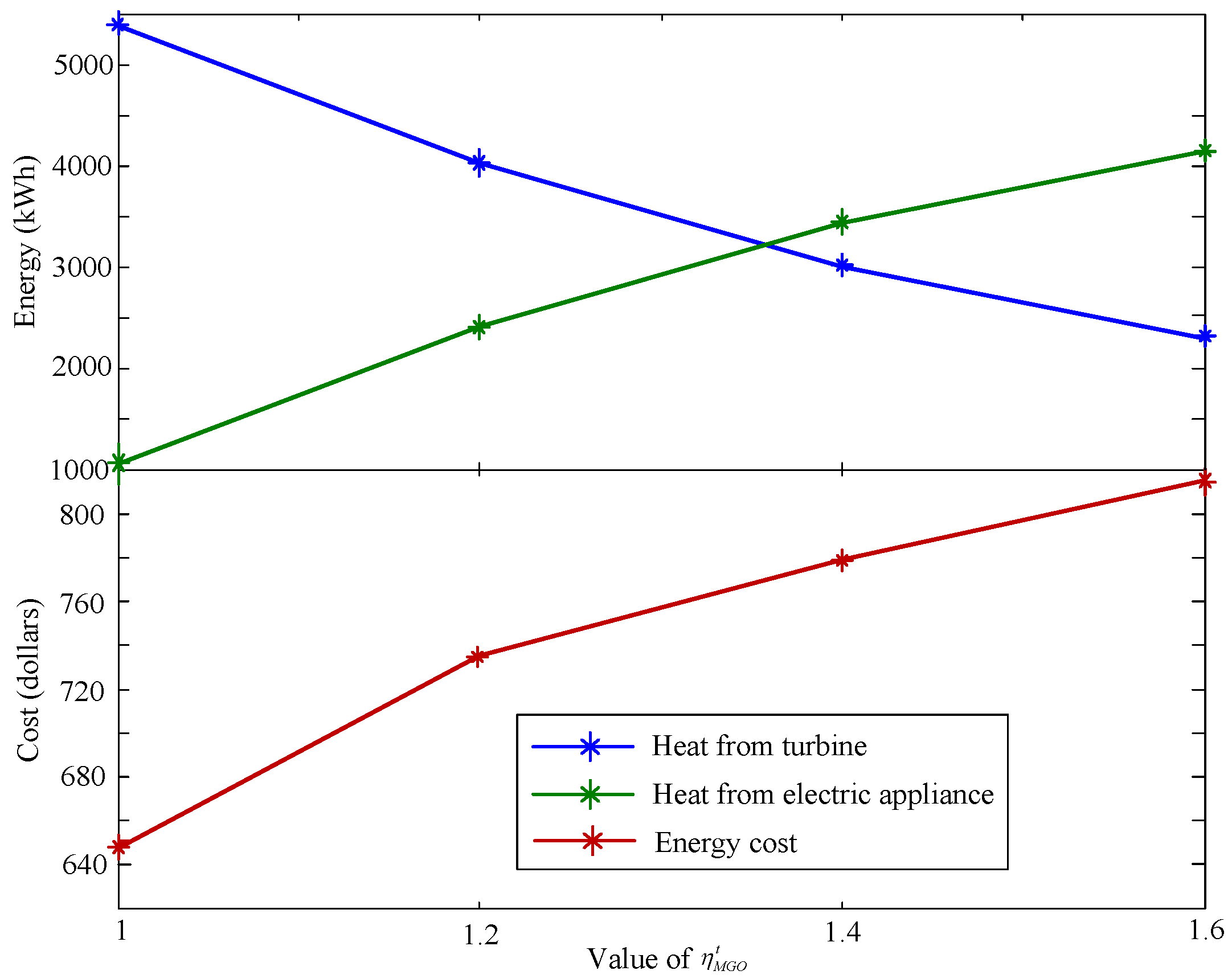
Figure 7 shows the whole thermal demand of a day and coalition’s cost when profit coefficient ${\eta }_{MGO}^t$ is varied from 1 to 1.6. From the figure, we can see that with the increasing of profit coefficient, prosumers will reduce the heat amount purchased from turbine for the lower energy cost. As a result, heat demand produced by electric appliance has a gradual increase. Due to the high profit pursuit of MGO in the trading, the daily cost of coalition increase in a certain rate, which are $648.58$ dollars with ${\eta }_{MGO}^t=1$, $738.46$ dollars with ${\eta }_{MGO}^t=1.2$, $783.27$ dollars with ${\eta }_{MGO}^t=1.4$, and $819.79$ dollars with ${\eta }_{MGO}^t=1.6$. When MGO adjusts the lease price from 0 dollars/kWh to 0.04 dollars/kWh, the charging amount of ESS and corresponding cost are shown in Figure 8. It is obvious that, with the increasing of lease price, prosumers have gradually reduced the leased capacity of ESS from MGO, and the daily charging amount of ESS is reduced dramatically from 2387 kWh to 1007 kWh. Consequently, prosumers will increase the energy amount purchased from public grid, whose energy cost from grid increases from 267.6 dollars (i.e., 39% in total cost) to 508.2 dollars (i.e., 61% in total cost). The above comparison results demonstrate that energy trading equilibrium strategy of prosumers will be affected greatly by MGO’s pricing mechanism.

6. Conclusions

In this paper, we proposed a day-ahead energy management framework for a community energy network considering the joint operation of CHP, shared ESS and prosumers. We have formulated an energy trading scheme where prosumers purchase energy from public grid or MGO, and store surplus energy to energy storage by renting the ESS of operator. In order to reduce daily energy cost, prosumers are willing to participate in the cooperation and DR project. Following which, a cooperative game model is founded for the coalition to optimize the energy consumption and purchasing strategies. After that, a distribution mechanism based on BSV is proposed to re-allocate the coalition cost into each prosumer. Simulation results have shown that the proposed scheme can effectively reduce daily costs for prosumers, while flatting the overall electricity demand on the public grid across the day. In addition, discussion and analysis are conducted from profit coefficient, shiftable loads’ percentage, and lease price of ESS. It demonstrates that MGO’s pricing results have a great influence on the optimal strategies and energy cost of prosumers.

Considering information network and EMS of residential users have not been completely promoted at the present stage, the proposed approach can be firstly applied to the micro demonstration project with perfect infrastructure, in which stakeholders are the operator of project and internal users. Additionally, the results in this paper can be extended in several directions. For example, the paper assumes that all prosumers only equips with electric appliance for thermal demand, without gas-based appliances, the following works may take gas load management into consideration. The effect of market is not considered in the proposed framework, further research may be conducted considering electricity and gas prices are influenced by market demand.

References

- Bao, Z.; Zhou, Q.; Yang, Z.; Yang, Q.; Xu, L.; Wu, T. A multi time-scale and multi energy-type coordinated microgrid scheduling solution-Part I: Model and methodology. IEEE Trans. Power Syst. 2015, 30, 2257–2266. [Google Scholar] [CrossRef]
- Ma, L.; Liu, P.; Fu, F.; Li, Z.; Ni, W. Integrated energy strategy for the sustainable development of China. Energy 2011, 36, 1143–1154. [Google Scholar] [CrossRef]
- Llaria, A.; Curea, O.; Jimlenez, J.; Camblong, H. Survey on microgrids: Unplanned islanding and related inverter control techniques. Renew. Energy 2011, 36, 2052–2061. [Google Scholar] [CrossRef]
- Palma-Behnke, R.; Benavides, C.; Lanas, F.; Severino, B.; Reyes, L.; Llanos, J.; Sáez, D. A microgrid energy management system based on the rolling horizon strategy. IEEE Trans. Smart Grid 2013, 4, 996–1006. [Google Scholar] [CrossRef]
- Milan, C.; Stadler, M.; Cardoso, G.; Mashayekh, S. Modeling of nonlinear CHP efficiency curves in distributed energy systems. Appl. Energy 2015, 148, 334–347. [Google Scholar] [CrossRef]
- Hawkes, A.; Leach, M. Cost-effective operating strategy for residential micro-combined heat and power. Energy 2007, 32, 711–723. [Google Scholar] [CrossRef]
- Zheng, X.; Wu, G.; Qiu, Y.; Zhan, X.; Shah, N.; Li, N.; Zhao, Y. A MINLP multi-objective optimization model for operational planning of a case study CCHP system in urban China. Appl. Energy 2018, 210, 1126–1140. [Google Scholar] [CrossRef]
- Li, L.; Mu, H.; Li, N.; Li, M. Economic and environmental optimization for distributed energy resource systems coupled with district energy networks. Energy 2016, 109, 947–960. [Google Scholar] [CrossRef]
- Wang, C.; Liu, Y.; Li, X.; Guo, L.; Qiao, L.; Lu, H. Energy management system for stand-alone diesel-wind-biomass microgrid with energy storage system. Energy 2016, 97, 90–104. [Google Scholar] [CrossRef]
- Gao, B.; Liu, X.; Zhang, W.; Tang, Y. Autonomous household energy management based on a double cooperative game approach in the smart grid. Energies 2015, 8, 7326–7343. [Google Scholar] [CrossRef]
- Mediwaththe, C.P.; Stephens, E.R.; Smith, D.B.; Mahanti, A. A dynamic game for electricity load management in neighborhood area networks. IEEE Trans. Smart Grid 2016, 7, 1329–1336. [Google Scholar] [CrossRef]
- Su, W.; Wang, J.; Roh, J. Stochastic energy scheduling in microgrids with intermittent renewable energy resources. IEEE Trans. Smart Grid 2014, 5, 1876–1883. [Google Scholar] [CrossRef]
- Gu, W.; Wang, Z.; Wu, Z.; Luo, Z.; Tang, Y.; Wang, J. An online optimal dispatch schedule for CCHP microgrids based on model predictive control. IEEE Trans. Smart Grid 2017, 8, 2332–2342. [Google Scholar] [CrossRef]
- Aghamohammadi, M.R.; Abdolahinia, H. A new approach for optimal sizing of battery energy storage system for primary frequency control of islanded microgrid. Int. J. Electr. Power Energy Syst. 2014, 54, 325–333. [Google Scholar] [CrossRef]
- Soliman, H.M.; Leon-Garcia, A. Game-theoretic demand-side management with storage devices for the future smart grid. IEEE Trans. Smart Grid 2014, 5, 1475–1485. [Google Scholar] [CrossRef]
- Palensky, P.; Dietrich, D. Demand side management: Demand response, intelligent energy systems, and smart loads. IEEE Trans. Ind. Inform. 2011, 5, 381–388. [Google Scholar] [CrossRef]
- Liu, X.F.; Gao, B.T.; Luo, J.; Tang, Y. Non-cooperative game based hierarchical dispatch model of residential loads. Autom. Electr. Power Syst. 20117, 41, 54–60. [Google Scholar]
- Yang, P.; Tang, G.; Nehorai, A. A game-theoretic approach for optimal time-of-use electricity pricing. IEEE Trans. Power Syst. 20113, 28, 884–892. [Google Scholar] [CrossRef]
- Bischi, A.; Taccari, L.; Martelli, E.; Amaldi, E.; Manzolini, G.; Silva, P.; Campanari, S.; Macchi, E. A detailed MILP optimization model for combined cooling, heat and power system operation planning. Energy 2014, 74, 12–26. [Google Scholar] [CrossRef]
- Han, G.; You, S.; Ye, T.; Sun, P.; Zhang, H. Analysis of combined cooling, heating, and power systems under a compromised electric-thermal load strategy. Energy Build. 2014, 74, 586–594. [Google Scholar] [CrossRef]
- Mehleri, E.D.; Sarimveis, H.; Markatos, N.C.; Papageorgiou, L.G. A mathematical programming approach for optimal design of distributed energy systems at the neighbourhood level. Energy 2012, 44, 96–104. [Google Scholar] [CrossRef]
- Ma, L.; Liu, N.; Zhang, J.; Tushar, W.; Yuen, C. Energy Management for Joint Operation of CHP and PV Prosumers Inside a Grid-Connected Microgrid: A Game Theoretic Approach. IEEE Trans. Ind. Inform. 2016, 12, 1930–1942. [Google Scholar] [CrossRef]
- Zhou, Z.; Liu, P.; Li, Z.; Ni, W. An engineering approach to the optimal design of distributed energy systems in China. Appl. Therm. Eng. 2013, 53, 387–396. [Google Scholar] [CrossRef]
- Chen, X.; Wang, Y.D.; Yu, H.D.; Wu, D.W.; Li, Y.; Roskilly, A.P. A domestic CHP system with hybrid electrical energy storage. Energy Build. 2012, 55, 361–368. [Google Scholar] [CrossRef]
- Wang, J.; Jing, Y.; Zhang, C. Optimization of capacity and operation for CCHP system by genetic algorithm. Appl. Energy 2010, 87, 1325–1335. [Google Scholar] [CrossRef]
- Atzeni, I.; Ordonez, L.; Scutari, G.; Palomar, D.P.; Fonollosa, J.R. Demand-side management via distributed energy generation and storage optimization. IEEE Trans. Smart Grid 2013, 4, 866–876. [Google Scholar] [CrossRef]
- Sarkar, S.; Ajjarapu, V. MW resource assessment model for a hybrid energy conversion system with wind and solar resources. IEEE Trans. Sustain. Energy 2011, 2, 383–391. [Google Scholar] [CrossRef]
- Karaki, S.; Chedid, R.; Ramadan, R. Probabilistic performance assessment of autonomous solar-wind energy conversion systems. IEEE Trans. Energy Convers. 1999, 14, 766–772. [Google Scholar] [CrossRef]
- Mohsenian-Rad, A.H.; Wong, V.M.S.; Jatskevich, J.; Schober, R.; Leon-Garcia, A. Autonomous demand-side management based on game-theoretic energy consumption scheduling for the future smart grid. IEEE Trans. Smart Grid 2010, 1, 320–331. [Google Scholar] [CrossRef]
- Baharlouei, Z.; Hashemi, M.; Narimani, H.; Mohsenian-Rad, H. Achieving optimality and fairness in autonomous demand response: Benchmarks and billing mechanisms. IEEE Trans. Smart Grid 2013, 4, 968–975. [Google Scholar] [CrossRef]
- Esmin, A.A.A.; Lambert-Torres, G.; De Souza, A.C.Z. A hybrid particle swarm optimization applied to loss power minimization. IEEE Trans. Power Syst. 2005, 20, 859–866. [Google Scholar] [CrossRef]
- Shapley, L.S. A value for n-person games. Contrib. Theory Games 1953, 2, 307–317. [Google Scholar]
- Javadi, F.; Kibria, M.R.; Jamalipour, A. Bilateral Shapley value based cooperative gateway selection in congested wireless mesh networks. In Proceedings of the IEEE Global Telecommunications Conference, New Orleans, LA, USA, 30 November–4 December 2008; pp. 1–5. [Google Scholar]
- Cui, P.; Shi, J.; Wen, F.; Sun, L.; Dong, Z.Y.; Zheng, Y.; Zhang, R. Optimal energy hub configuration considering integrated demand response. Electr. Power Autom. Equip. 2017, 37, 101–109. (In Chinese) [Google Scholar]
- Kerdphol, T.; Fuji, K.; Mitani, Y. Optimization of a battery energy storage system using particle swarm optimization for stand-alone microgrids. Int. J. Electr. Power Energy Syst. 2016, 81, 32–39. [Google Scholar] [CrossRef]
- Liu, X.; Gao, B.; Wu, C.; Tang, Y. Demand-Side Management With Household Plug-In Electric Vehicles: A Bayesian Game-Theoretic Approach. IEEE Syst. J. 2017, 1–11. [Google Scholar] [CrossRef]
Figure 1.
Structure of community energy network.
Figure 2.
Typical loads and energy output of PV.
Figure 3.
Optimal result of electrical energy: (a) is dispatching result of electricity energy resource; (b) is scheduling result of total electrical load.
Figure 4.
Optimal result of thermal energy.
Figure 5.
Daily cost along with the iterations of the algorithm.
Figure 6.
Electrical load curve for different percentages of shiftable loads.
Figure 7.
Thermal demand and cost for different values of profit coefficient.
Figure 8.
Charging amount of ESS and cost for different lease price of ESS.