Model for Estimation of Fuel Consumption of Cruise Ships

Abstract

This article presents a model to estimate the energy use and fuel consumption of cruise ships that sail Norwegian waters. Automatic identification system (AIS) data and technical information about cruise ships provided input to the model, including service speed, total power, and number of engines. The model was tested against real-world data obtained from a small cruise vessel and both a medium and large cruise ship. It is sensitive to speed and the corresponding engine load profile of the ship. A crucial determinate for total fuel consumption is also associated with hotel functions, which can make a large contribution to the overall energy use of cruise ships. Real-world data fits the model best when ship speed is 70–75% of service speed. With decreased or increased speed, the model tends to diverge from real-world observations. The model gives a proxy for calculation of fuel consumption associated with cruise ships that sail to Norwegian waters and can be used to estimate greenhouse gas emissions and to evaluate energy reduction strategies for cruise ships.

1. Introduction

Global use of heavy oil and diesel for ships makes a small contribution to climate change−some 2.2% of global emissions of CO₂ on the order of 795–938 Mt CO₂ in 2012 [1]. The most recent model suggests emissions of 831 Mt CO2 in 2015 [2]. The shipping sector is projected to grow by 50–250% by 2050 [1], where emissions from all other sectors except aviation are expected to fall under the Paris Agreement. Growth of shipping emissions has already prompted calls to introduce market-based measures in the shipping sector to increase the cost of emissions [3]. Notably, shipping will also be affected by climate policy because under low-carbon scenarios, there will be a steep decline in the supply of oil that is still traded by the shipping industry [4,5].

Cruise ships account for only a small share of the global shipping emissions, though they are increasingly discussed in other sustainability contexts, specifically concerning local and regional air pollution [6,7,8]. The cruise ship sector has seen significant growth in recent years [9], with expectations that these trends will continue. Cruise Market Watch [10] reports, for example, that 13 new cruise ships will enter the market in 2018, and another 37 by 2020. Cruise ships carried some 23 million passengers in 2015 [9] and are expected to carry 27.6 million by 2020 [10]. Though cruises are only a small segment of global tourism, they represent the most energy intense form of tourism on a per passenger-km basis [11]. Overall, the sector contributed emissions of 35 Mt CO₂ in 2012, up from 27.8 Mt CO₂ in 2007 [1]. This increase has prompted research into the environmental sustainability of cruise tourism [12,13,14,15,16] and has resulted in calls to regulate the sector, specifically with regard to climate change [17,18]. Currently, various policies at international, regional, national, and even local level are about to be implemented, including the EU monitoring, reporting, and verification initiative entering into force in July 2015 [19] and the International Maritime Organization’s (IMO) data collection system, starting in March 2018. Additional international-level policies are being discussed [3,20], with calls for significantly improved emission inventories [21]. A number of national and local initiatives are also in place, notably policy measures on low-transport and low-impact zoning, substitution of fossil fuels with alternative fuels, and on shore power.

Three basic approaches to reducing shipping emissions have been outlined in the literature, including managerial, technological, and policy options [22]. For example, cruise operators have some degree of freedom in the identification of attractive destinations and the design of routes. Cruise ships also have some flexibility with regard to the speeds at which they move, weather routing, and autopilot adjustments [23,24]. Ship design as well as propulsion technologies can also make significant contributions to reducing emissions. Hull shapes, air lubrication or low friction hull coatings, engine tuning, propeller polishing, water flow-optimisation at hull openings, the use of propeller boss caps with fins, speed control of pumps and fans, main engine tuning, shore-side electricity, as well as liquefied natural gas (LNG) or biodiesel replacing oil and diesel have all been discussed with regard to their potential to reduce emissions [23]. Several of these technologies are already in use in cruise ships [25], and their market introduction may be stepped up by emerging marine policies such as CO₂ taxes or emission-control areas (ECA). In port cities, which often face high levels of air pollution from ships, the discussion of policies is particularly intense [26,27].

In spite of many proposed strategies for reduction in shipping emissions, the contribution made by individual or combined managerial and technological strategies to mitigation is still difficult to assess. There continues to be uncertainty regarding fuel consumption of individual ships under various operational conditions [23]. To assess emissions from global shipping, the IMO relies on top down and bottom-up estimates, noting that “In addition to the uncertainties behind the total shipping emissions and fuel type allocations in each year, both methods contain separate but important uncertainty about the allocation of fuel consumption and emissions to international and domestic shipping” ([1], p. 10). These uncertainties have also been observed in the context of other approaches to assess emissions. For example, Moreno-Gutiérrez et al. [28] compared nine inventory methodologies (TNO [29], Entec [30], Ship Traffic Emission Assessment Model [STEAM] [31], Environmental Protection Agency [32], Corbett and Koehler [33], Eyring [34], IMO [35,36]) to calculate energy consumption and associated emissions of ships passing through the Strait of Gibraltar. They found considerable variation in results (up to 27%) that they linked to engine use ratios (main to auxiliary) as well as to engine loads. Moreno-Gutiérrez et al. [28] also highlight uncertainties resulting out of emission inventory assumptions on the basis of manufacturer test data or national data use (i.e., averages that are not characteristic of a specific local situation). Refined models are consequently warranted to better assess fuel consumption under different operational and environmental conditions.

In their review, Moreno-Gutiérrez et al. [28] concluded that the most reliable emission assessment model is the Ship Traffic Emission Assessment Model (STEAM), which uses Automatic Identification System (AIS) data to track ship movements at high spatial and temporal resolutions. AIS data is preferable for modelling, as it provides exact data on the location of ships at a given time, hence allowing for calculations of speeds or port times. AIS data has been used in a wide range of publications seeking to assess emissions, including Jalkanen et al. [31,37] in the Baltic Sea; Ng et al. [38] in Hong Kong, Johansson et al. [39] for the Northern European Control Area, Goldsworthy and Goldsworthy [40] in Australia, Aulinger et al. [41] in the North Sea [2], and Smith et al. [1] for global shipping. Johansson et al. [2] use a refined version of STEAM (STEAM3) that compensates for missing information on technical specifications, scarcity of satellite data in some regions, and other refinements and allows for modelling of emission control areas. Yet, models continue to be characterized by methodological difficulties, such as to account for specific marine conditions (e.g., draught), extreme weather events, fuel types, or engine load factors, all of which have importance for emissions. Specifically, in the context of cruise ships, existing emission estimates have largely relied on bunker fuel data released by cruise operators or calculations of average emission factors [11,42].

In this article, a model is built to estimate fuel consumption associated with cruise ships sailing Norwegian waters. Fuel estimation is based on IMO’s third greenhouse gas (GHG) emissions study [1]; i.e., the paper assesses whether this formula is also valid for passenger cruise ships. The IMO formula has been shown to have good agreement for a merchant fleet (i.e., tanker and container ships) [1]. However, it was not tested against cruise ships, which have highly variable power systems. Cruise ships have mechanical and diesel-electric power systems as well as hybrid variants or so-called “geared systems”. For diesel-electric and hybrid systems, the main engine power is also shared with auxiliary or hotel power. For this reason, the IMO formula is compared with real-world data and then tested against a small cruise vessel, a medium cruise ship, and a large cruise ship. The model is based on AIS data obtained from the Norwegian coastal authority as well as on specific technical information from the SeaWeb database. In addition, information about port emissions obtained from questionnaires filled out by cruise companies and obtained from a fuel-monitoring system has been incorporated.

2. Model Description

The data set contains geographical locations as well as speed measured at different time intervals for each cruise ship entering Norwegian waters in 2016. The time interval is by default 5 min, but this may vary. The data are measured per ship per month.

In the model, speed registrations between two consecutive geographical locations are interpolated to correct for different time intervals between registrations. This means that all speed and fuel consumption calculations are made for the same time unit, which is one minute.

For each ship, time spent in port is also measured on the same time interval. This makes it possible to have different algorithms for calculating fuel consumption for different modes such as operations in open sea, manoeuvring into port and staying in port.

As part of this project, a database with information for 169 cruise ships based on information from SeaWeb has been created. The database covers all the ships operating in Norwegian waters in 2016. It contains information about ship properties such as gross weight, berths, year built, power rating based on MCR (maximum continuous rating), machine configuration (i.e., diesel-electric or not), number of main and auxiliary engines and generators, numbers and type of propellers, and service and maximum speed.

2.1. Calculating Time Span between Registrations

For every two registrations for one cruise ship the number of minutes between these registrations are calculated. The number of minutes is then used for calculating the amount of time an engine load has been applied. This again gives the energy consumption in, for example, kilowatt-hours.

The calculation of minutes must take into consideration that the time span between two registrations may cover one day or two consecutive days. If both time registrations are for the same day, minutes according to Equation (1) are calculated, where t₀ is the first of two consecutive time registrations and t₁ is the last. Minutes between two consecutive time registration on the same day is defined as follows:

$$\mathrm{minutes}=\left({\mathrm{hour}}_{\mathrm{t}1}\times 60+{\mathrm{minutes}}_{\mathrm{t}1}\right)-({\mathrm{hour}}_{\mathrm{t}0}\times 60+{\mathrm{minutes}}_{\mathrm{t}0})$$

(1)

If the two time registrations are for two consecutive days, minutes until midnight have to be calculated for the first day. Minutes between two consecutive time registrations on two consecutive days is defined as follows:

$$\mathrm{minutes}=\left\{{\mathrm{hour}}_{\mathrm{t}1}\times 60+{\mathrm{minutes}}_{\mathrm{t}1}\right\}-\left\{{\mathrm{TotMin}}_{\mathrm{day}1}-\left({\mathrm{hour}}_{\mathrm{t}0}\times 60+{\mathrm{minutes}}_{\mathrm{t}0}\right)\right\}$$

(2)

TotMin_day1 is the total number of minutes on first day, e.g., 1440 min. If the time span between the two consecutive time registrations is more than one day, number of minutes in the above equation is set to 1 min. Since registrations refer to Norwegian waters, cruise ships may return to a port outside this area, e.g., Hamburg, in order to pick up new passengers. For the following first registration in Norwegian waters a 1 min sailing time with the registered speed is assumed.

2.2. Calculating Distance between Two Latitudes and Longitudes

The haversine formula is used to calculate the distance between two pairs of latitude and longitude combinations [43]. First, the differences between latitudes and longitudes are found and converted to radians. This is shown in Equations (3) and (4) where Lat_t0 is the first latitude registration and Lat_t1 is the second. The same logic applies to longitudes. Difference between latitudes to radians is defined as follows:

$$\mathrm{dLat}=\frac{\left({\mathrm{Lat}}_{\mathrm{t}1}-{\mathrm{Lat}}_{\mathrm{t}0}\right)\times \mathsf{\pi }}{180}$$

(3)

Difference between longitudes to radians is defined as follows:

$$\frac{\left({\mathrm{Lng}}_{\mathrm{t}1}-{\mathrm{Lng}}_{\mathrm{t}0}\right)\times \mathsf{\pi }}{180}$$

(4)

Each latitude in the two pairs is also turned into a radian, as shown in Equation (5) where the subscript i symbols each of the two latitudes in the pair. The equation produces variables Lat1_rad and Lat2_rad. Latitude to radian is defined as follows:

$${\mathrm{Lat}}_{\mathrm{rad},i}=\frac{\left({\mathrm{Lat}}_i\right)\times \pi }{180}$$

(5)

Left hand side variable a in Equation (6) refers to the square of half the chord length between the points and the corresponding variable c in Equation (7) refers to the angular distance in radians. Square of the chord length between latitude and longitude points is defined as:

$$\mathrm{a}={\left(\frac{\sin \left(\mathrm{dLat}\right)}{2}\right)}^2+{\left(\frac{\sin \left(\mathrm{dLon}\right)}{2}\right)}^2+\cos (\mathrm{Lat}{1}_{\mathrm{rad}})+\cos \left(\mathrm{Lat}{2}_{\mathrm{rad}}\right)$$

(6)

Angular distance between radians is defined as:

$$\mathrm{c}=2\times \mathrm{atan}2\left(\sqrt{\mathrm{a}},\sqrt{\left(1-\mathrm{a}\right)}\right)$$

(7)

In Equation (7), atan2 is arctangent function. Finally, the distance between two pairs of latitudes and longitudes in meters can be found based on Equation (8). Distance between pairs of latitudes and longitudes in meters is defined as follows:

$$\mathrm{m}=\mathrm{R}\times \mathrm{c}\times 1000$$

(8)

In Equation (8) R is the diameter of the Earth, 6371 km.

2.3. Interpolation

Two interpolation algorithms are implemented in order to calculate speed between two consecutive time registrations. Interpolation of speed is based on a current speed for a given point in time and the speed at the previous time registration. The last speed is referred to as base speed and the first is the target speed. If base speed is zero, a linear interpolation is used. If base speed is larger than zero, an exponential algorithm is used.

For both interpolations, the difference between the target speed (TS) and the base speed (BS) is identified. The number of minutes between the two speed registrations is calculated as described in Equations (1) and (2).

The linear interpolation is used when the base speed is zero. This usually occurs when ships are leaving a port. The linear interpolation is therefore mostly used for manoeuvring speed inside or just outside ports.

A linear interpolation according to Equation (9) is implemented where the symbol TS is the target speed at interpolation end point, BS is the base speed at the interpolation start point, t is the number of minutes from interpolation start point, S_t is interpolated speed at time t and totMin are minutes taken from calculations above in Equation (1) or Equation (2). The linear interpolation is defined as follows:

$${\mathrm{S}}_{\mathrm{t}}=\mathrm{BS}+\frac{\left(\mathrm{TS}-\mathrm{BS}\right)}{\left(\mathrm{totMin}\right)}\times \mathrm{t}$$

(9)

As an example, the cruise ship Norwegian Star left the port in Ålesund, Norway on 3 May 2016, at 16:10. At 16:15, the ship had a speed of 4.2 knots. To identify the speed 3 min after the first registration, 5 min between the base speed at 0 knots and the target speed at 4.2 knots represent an increase of 4.2/5 = 0.84 knots per minute between the two speed registrations. For the 3 min, this is 0 + 0.84 × 3 = 2.52 knots.

The distance that a ship covers when manoeuvring is very small. Yet, calculations for manoeuvring can give very high fuel consumption because the ship may move less than 1 nautical mile at that speed. This was the case for Norwegian Star registrations on 19 May 17:15 when the ship left Ålesund harbour. During the 5-min interval from previous registration, the ship only moved some 100 m. Interpolation for every minute in this interval results in very high fuel consumption per nautical mile. To correct for this, fuel consumption is calculated only for movements larger than a quarter of a nautical mile, approximately 460 m. This rule is implemented to exclude extreme fuel consumption over short distances while manoeuvring in port.

Exponential interpolation is used when both base and target speed is above zero and the number of days between two consecutive registrations is no more than 1. When the number of days is larger than 1 it is assumed that the ship has left Norwegian waters and then entered again some days later. In that case the number of minutes for the first registration when re-entering Norwegian waters is 1 and not interpolated.

By using exponential interpolation, speed is accelerating the closer the ship is to the target speed; and de-accelerating when it is slowing down.

In Equation (10) the interpolation factor (IF) between the two speeds is identified. This factor represents the expected increase (or decrease) for every minute. The number of minutes is calculated as described above in Equations (1) and (2). Interpolation factor for exponential interpolation is defined as follows:

$$\mathrm{IF}={\left(\frac{\mathrm{TS}}{\mathrm{BS}}\right)}^{\left(\frac{1}{\mathrm{minutes}}\right)}$$

(10)

The formula for exponential interpolation is depicted in Equation (11) where BS is base speed, IF the interpolation factor from Equation (10), t the number of minutes from base speed registration and S_t interpolated speed at time t. Exponential interpolation is defined as follows:

$${\mathrm{S}}_{\mathrm{t}}=\mathrm{BS}\times {\mathrm{IF}}^{\mathrm{t}}$$

(11)

On 20 May at 17:20, Norwegian Star was just outside Valle in Sunnmøre region, Western Norway. This is on the entrance to the Storfjord which leads to the Geiranger port, one of the most popular cruise destinations in Norway. The ship’s speed was 17.3 knots. The previous speed registration was 17.2 knots at 17:15, 1.44 nautical miles to the west. To find the speed 3 min from the base speed registration, an interpolation factor is used (17.3/17.2 = 1.0058). This factor is taken to the power of 1/5 (where 5 is number of minutes between registrations), resulting in an increase in speed of 1.001 knots per minute. Calculation of the speed at 3 min from base speed registration results in 17.2 × (1.001³) = 17.26 knots.

Speed between every two registrations was calculated, as well as fuel consumption for all intermediate speeds because the time interval may vary. For instance, the Norwegian Star was registered with a speed of 15 knots on 7 May at 15:40. The previous speed registration was 14.9 knots, at 15:25. On 18 September, the same ship was registered with a speed of 15.5 knots at 04:10. The previous registration was 38 min earlier at 03:32 (15 knots). Even if the speed difference is minor between the two registrations, interpolation between them will yield a uniform approach to fuel calculations independent of the variations in time span between two registrations.

The underlying problem is that there are missing gaps in the data set generated by the Norwegian Coastal Authority because registrations do not always have the same time span between them. When speed interpolation is applied to all registrations and fuel consumption calculated for all interpolated speed values, these gaps will not lead to biases in fuel calculations.

2.4. Algorithm for Calculating Fuel Consumption at Sea

The algorithm is based on the following steps:

• Apply a speed cut-off value of 4 knots. If the ship is traveling above that speed, it is cruising at open sea. Otherwise, it is in port or is manoeuvring in port. The cut-off value has been discretionary set after inspecting several cruise ships’ speed distribution when entering or leaving a port.
• Find the load on the power rating necessary to attain a given speed. The load is the proportion of total installed power (kW) in use.
• Calculate the applied power rating in kilowatt (kW) using the calculated load.
• Calculate the time span for that speed in knots.
• Combine the actual power applied with the elapsed time span for that power in order to calculate power consumption in kilowatts per hour (kWh).
• Add fuel consumption for hotel functions in open sea.
• Aggregate the calculated fuel consumption for the time a cruise ship spent in open sea per month.

Fuel consumption at sea is only calculated if the recorded speed is larger than 4 knots. For speed records below this limit, the ship is assumed to be in port or manoeuvring.

Equation (12) is taken from the Smith et al. ([1] p. 177) It is used to calculate the power rating required to attain a given speed for a given ship at a given location. Applied power for a given speed is defined as:

$${\mathrm{P}}_{\mathrm{t}}=\frac{{\mathrm{P}}_{\mathrm{ref}}{\left(\frac{{\mathrm{D}}_{\mathrm{t}}}{{\mathrm{D}}_{\mathrm{ref}}}\right)}^{\left(\frac{2}{3}\right)}{\left(\frac{{\mathrm{V}}_{\mathrm{t}}}{{\mathrm{V}}_{\mathrm{ref}}}\right)}^{\mathrm{n}}}{{\mathsf{\tau }}_{\mathrm{w}}{\mathsf{\tau }}_{\mathrm{f}}}$$

(12)

where P is engine power, V is speed and D is draught while t is measurements for these properties at time t and ref indicates reference values for the same properties. The reference value for speed is the ship’s service speed [44]. The symbol ${\mathsf{\tau }}_{\mathrm{w}}$ is a constant (1.15) allowing for the effect of weather on propulsion efficiency while ${\mathsf{\tau }}_{\mathrm{f}}$ is a constant describing the effect of fouling on the same efficiency (1.09). The value n is the ratio of speed and power and has a constant value of 3.

Draught data for cruise ships are not collected in the same time interval as speed data, and as a result draught registrations for a specific cruise ship cannot be joined with its speed registrations. According to US Navigation Center [45], draught is measured in decimetres (1/10 m), but the exact point of measurement on the ship (e.g., bow, amidships or stern), is undefined. Some ships have static draught which means that its measurement does not change during sailing. Therefore, draught registrations should be taken more as indications as real time measurements. Here, the draught factor is defined as a ratio of the minimum registered draught for a ship over its maximum as shown in Equation (13). Several ships are registered with obviously ‘wrong’ draughts. For example, the cruise ship Mein Schiff 1 is registered with a draught of 0.1 on 5 September, at 19:36:43. At this time, the ship was sailing in the outer parts of the Oslofjord, approximately at the position latitude = 58.915, longitude = 10.488. There are several registrations for this ship with draughts below 1, which is obviously wrong. In the database, the 90th percentile for the ratio of maximum registered draught to the minimum one has a value of 1.785. The model assumes that no draught for a given ship can be less than 1/1.785 of the maximum registered draught for that ship. The draught factor is defined as follows:

$$\frac{{\mathrm{D}}_{\mathrm{t}}}{{\mathrm{D}}_{\mathrm{ref}}}=\frac{{\mathrm{D}}_{\min }}{{\mathrm{D}}_{\max }}$$

(13)

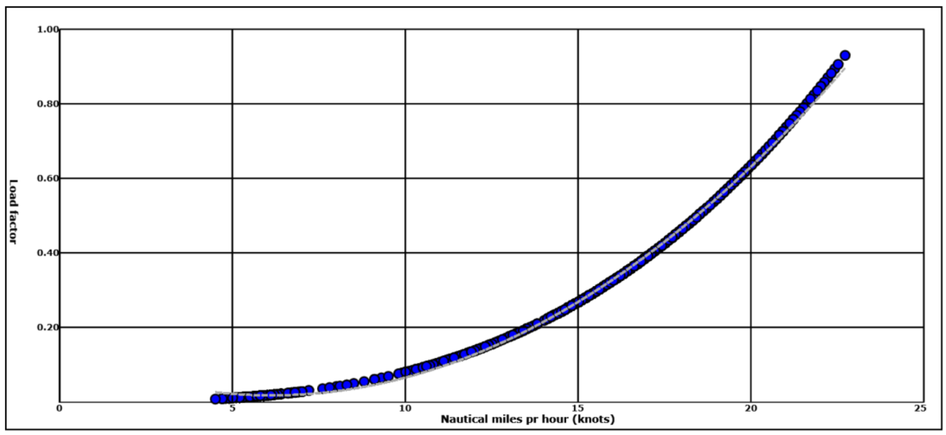
Equation (12) will provides the applied power in kW for a given speed. Since the installed engine power for each ship is known, the load factor for that speed can be calculated, as shown in Equation (14). Instantaneous load factor is defined as follows:

$${\mathrm{L}}_{\mathrm{t}}=\frac{{\mathrm{P}}_{\mathrm{t}}}{{\mathrm{P}}_{\mathrm{ref}}}$$

(14)

${\mathrm{L}}_{\mathrm{t}}$ is the instantaneous load factor at time t required to produce the power necessary to attain a given speed.

For diesel-electric ships, the reference power is calculated using a propulsion factor. The propulsion power is defined as the sum of power yield for each electric motor. This power as a proportion of total power is defined as the propulsion factor for diesel-electric ships. The assumption is that these ships use a proportion of total power for auxiliary purposes such as lightning, HVAC (Heating, Ventilation and Air Conditioning), and hot water provision. The propulsion power then measures the proportion of total power exclusively used for propulsion; the remainder (1 minus the propulsion factor) being used for auxiliary purposes. Propulsion factor is defined as follows:

$$\mathrm{PF}=\left(\frac{{{\displaystyle \sum }}_{i=1}^n{\mathrm{EP}}_i}{\mathrm{TP}}\right)$$

(15)

Reference power for diesel-electric ships is defined as follows:

$${\mathrm{P}}_{\mathrm{ref}}=\mathrm{PF}\times \mathrm{TP}$$

(16)

Equation (15) shows the formula for finding PF, the propulsion factor. In the equation, EP_i is the power of the i’th electric motor, n is number of electric motors, TP is the ship’s total power. The propulsion factor PF is then used in Equation (16) to find the reference power for diesel-electric ships.

The next step is to calculate specific fuel consumption based on the load factor at time t. The specific fuel consumption is taken from Smith et al. ([1], p. 110). Instantaneous specific fuel consumption is defined as follows:

$${\mathrm{SFC}}_{\mathrm{t}}={\mathrm{SFC}}_{\mathrm{base}}\times \left(1.28-\left(0.71\times {\mathrm{L}}_{\mathrm{t}}\right)+\left(0.455\times {\mathrm{L}}_{\mathrm{t}}{}^2\right)\right)$$

(17)

Equation (17) calculates the instantaneous fuel consumption at time t given a baseline and the load factor from Equation (14). The baseline is taken from Smith et al. (Table 49 in [1] p. 109). It gives the baseline fuel consumption in g/kWh for high speed diesel engines built in different periods. The table is reproduced in

Table 1. Baseline fuel consumption for high speed diesel engines.

Year Built	Baseline in g/kWh
Before 1983	225
1984–2000	205
post 2001	195

.

The final step is to calculate the time span for the fuel consumption in Equation (17). This is done by calculating the minutes between two speed registrations for a cruise ship. The minutes are converted into hours to derive an estimated kWh for a given kW. Instantaneous kWh is defined as follows:

$${\mathrm{kWh}}_{\mathrm{t}}={\mathrm{P}}_{\mathrm{t}}\times \frac{\left({\mathrm{m}}_{\mathrm{t}}-{\mathrm{m}}_{\mathrm{t}0}\right)}{60}$$

(18)

Equation (18) gives the calculated kWh at a time t. The symbol t₀ is the previous time registration and the value for P_t is taken from Equation (12). Instantaneous fuel consumption in tons is defined as follows:

$${\mathrm{F}}_{\mathrm{t}}={\mathrm{kWh}}_{\mathrm{t}}\times {\mathrm{SFC}}_{\mathrm{t}}$$

(19)

Equation (19) shows calculation of fuel consumption at time t (F_t) based on instantaneous kilowatt-hours and instantaneous specific fuel consumption (SFC_t) taken from Equation (17).

2.5. Algorithm for Calculating Fuel Consumption in Port

Previous studies have shown that the fuel consumption for hotel functions (such as ventilation, lightning, and hot water) could be substantial for cruise ships, on average about 40% of total energy consumption [42]. However, large differences are found between individual ships within the same size [46,47]. Our algorithm is based on three sources: (a) a survey of fuel consumption in port for cruise ships in Skagway, Alaska, in 2008 [46], (b) a survey based on cruise ships that sailed to the world heritage area fjords in Norway in 2017 [47], (c) as well as real world data obtained from the ship MS Finnmarken from May 2016 to September 2017. We assume that fuel consumption for hotel functions is identical in port and in open sea [48,49]. The Alaska report is based on information from 11 different cruise ships. Stays in port are defined as speed registrations less than or equal to 4 knots.

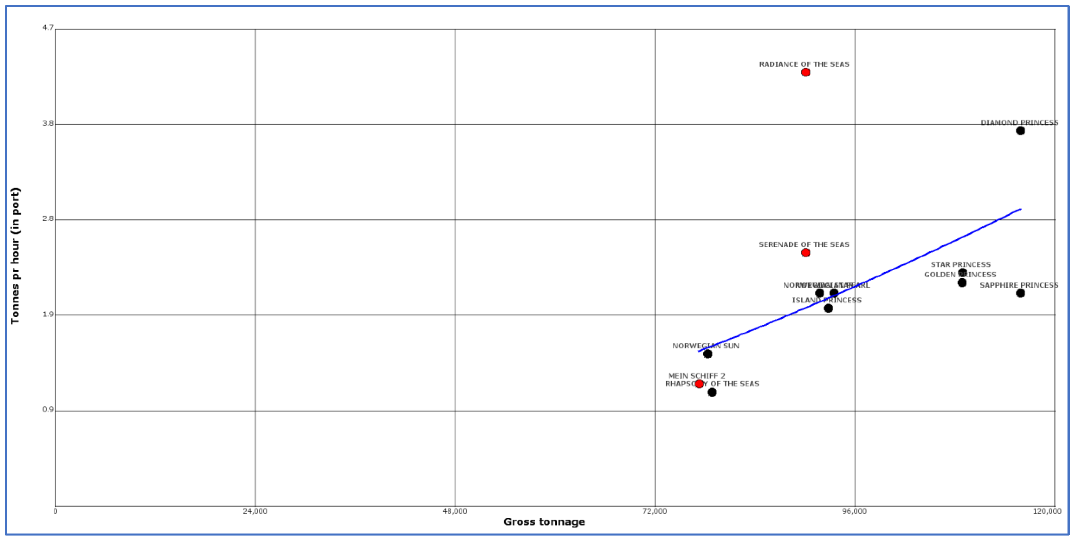
Figure 1 shows the estimated relationship between gross weight and tons of fuel per hour spent in port for the cruise ships in the Alaska report. Ships with a diesel-electric configuration are represented by black dots and other ship types by red dots.

We have applied a multivariate regression model shown in Equation (20) where the $\mathsf{\beta }$’s represent regression coefficients and $\mathsf{\epsilon }$ is a well-behaved residual term. The variables in the model are defined in

Table 2. Multivariate regression model for hotel functions.

Type	Name	Description
Dependent	FuelTonsPrHour	Tonne of fuel per hour spent in port for hotel functions
Independent	GrossWeight	Gross weight in tons
Independent	Berths	Number of berths
Independent	DummyDieselElectric	1 if the ship has a diesel-electric configuration, otherwise 0

. We have assumed a log-log relationship between tons per hour and the independent variables gross weight and berths. This means that the regression coefficients measure the percentage effect on fuel consumption from one percent change in the independent variables.

The estimated multivariate regression model is defined as:

$$\ln \left(\frac{{\mathrm{fuel}}_{\mathrm{tonnes}}}{\mathrm{hour}}\right)={\mathsf{\beta }}_0+{\mathsf{\beta }}_1\times \ln \left(\mathrm{GrossWeight}\right)+{\mathsf{\beta }}_2\times \ln \left(\mathrm{Berths}\right)+{\mathsf{\beta }}_3\times {\mathrm{Dummy}}_{\mathrm{diesel}-\mathrm{electric}}+\mathsf{\epsilon }$$

(20)

Based on regression coefficients from the estimated model the fuel consumption tons per hour in port can be obtained:

$$\frac{{\mathrm{Fuel}}_{\mathrm{tonne}}}{\mathrm{hour}}={\mathrm{e}}^{\left(-21.9+\left(2.8\times \ln \left(\mathrm{GrossWgt}\right)\right)+\left(-1.15\times \ln \left(\mathrm{berths}\right)\right)+\left(-0.36\times {\mathrm{Dummy}}_{\mathrm{Diesel}-\mathrm{electric}}\right)\right)}$$

(21)

We find the total fuel consumption for a stay in port by multiplying tons per hour with the actual stay in hours.

Table 3. Data for fuel consumption in port from Skagway-report.

Ship	Gross Weight	Berths	Tons per hour in Port Skagway (A)	Dummy (1 = Diesel Electric)	Hotel Load MW (B)	g/kWh C = (A/B) × 1000
Norwegian Star	91,740	3000	2.1	1	9	233
Serenade of the Seas	90,090	2500	2.5	0	5.5	454
Rhapsody of the Seas	78,878	2417	1.125	1	5.3	212
Island Princess	92,822	2581	1.95	1	7.2	271
Radiance of the Seas	90,090	2495	4.275	0	5.3	807
Norwegian Pearl	93,530	3130	2.1	1	7.2	292
Star Princess	108,977	3300	2.3	1	10.5	219
Golden Princess	108,865	3300	2.2	1	10.5	210
Diamond Princess	115,906	3100	3.7	1	11.5	322
Norwegian Sun	78,309	2450	1.5	1	5.6	268
Mein Schiff 2	77,302	2681	1.2	0	4.1	293
SapphirePrincess	115,875	3078	2.1	1	9.6	219

shows the data set used for estimating the multivariate regression model in Equation (20).

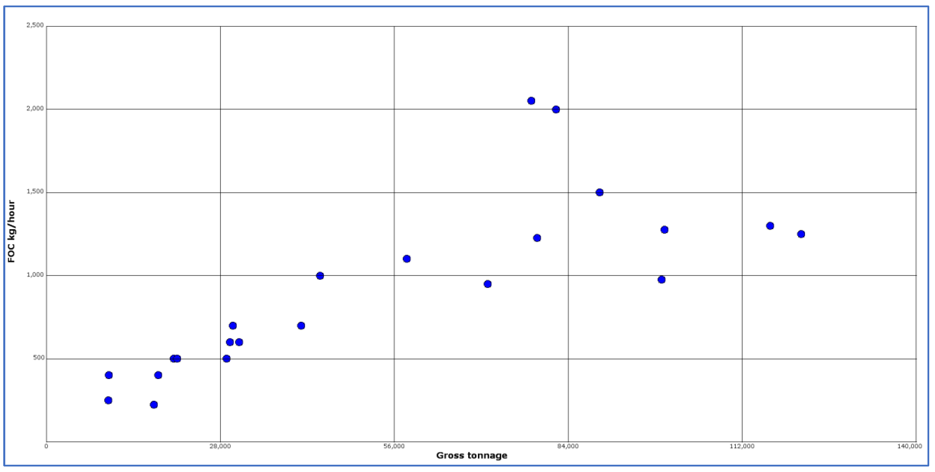
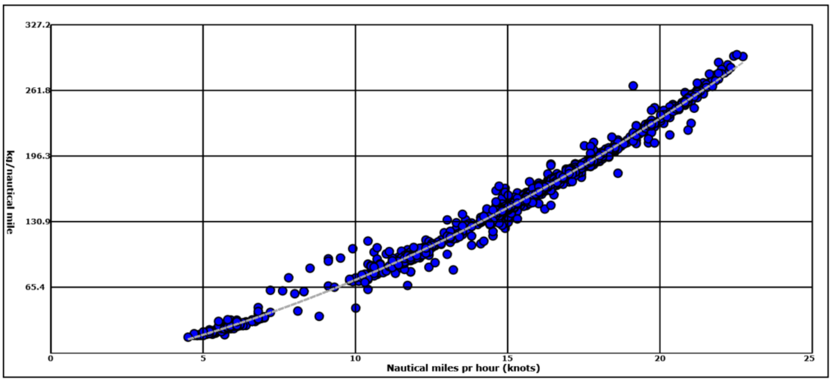
The smallest ship in the Alaska survey measured by gross tons is Mein Schiff 2 (earlier called Celebrity Mercury) with 77,302 tons. Accordingly, using a model based on these data items to predict fuel consumption for smaller ships, their consumption may be underestimated since the trend line in Figure 1 will be extrapolated downwards towards the x-axis. The Norwegian research company Marintek [47] made a survey of cruise ships in Norwegian world heritage fjords in 2017. Based on responses to that survey Marintek published a figure (Figure 5.11 in [47]) of fuel consumption in kg per hour against gross weight for ships in the range 10,000 to 121,000 gross tons. Marintek will not make their underlying data public, but from the figure it is possible to roughly read pairs of data for gross tons and fuel consumption.

Figure 2 can be used to estimate a rough function. For this, a log-log model with kg per hour as dependent and gross tons as independent variable was developed. The estimated fuel consumption in port from the Marintek study gives the following coefficients:

$$\frac{{\mathrm{Fuel}}_{\mathrm{tonne}}}{\mathrm{hour}}={\mathrm{e}}^{\left(-0.88+(0.71\times \ln \left(\mathrm{GrossWgt}\right)\right)}$$

(22)

The Marintek study shows that no cruise ships larger than 90,000 gross tons have a fuel consumption larger than 1.5 tons per hour. This corresponds poorly with the Alaska study [43] where none of the ships with the same size have a fuel consumption below 1.9 tons per hour. A main reason for this difference is that the Marintek study applies 200 g of fuel per kWh, compared to an average of 272 g/kWh in the Alaska study. The difference is 26.4 percent between the two models for ships over 70,000 gross tons. For smaller ships below 70,000 gross tons, the Marintek study provides more reliable estimates. It is known that extrapolation of regression analysis from large values to lower values may lead to an underestimation of lower values. For the cruise ship Artania with 44,656 gross tons, the Marintek study estimates 805 kg of fuel per hour while the same extrapolated estimate from the Alaska study is 443 kg per hour. We will therefore use coefficients from the Alaska study for cruise ships above 70,000 tons and coefficients from the Marintek study for ships in the range 25,000 to 70,000 gross tons. For ships below 25,000 gross tons we will use estimates based on actual data from MS Finnmarken which is a smaller cruise ship operated by the Norwegian company Hurtigruten (see next section). Fuel consumption in port is calculated as follows:

$${\mathrm{Fuel}}_{\mathrm{in}-\mathrm{port}-\mathrm{tonne}}=\frac{{\mathrm{Fuel}}_{\mathrm{tonne}}}{\mathrm{hour}}\times {\mathrm{hours}}_{\mathrm{in}-\mathrm{port}}$$

(23)

To estimate fuel consumption for hotel functions at sea, expected fuel consumption in tons per minute is calculated by dividing tons per hour by 60. Fuel consumption per minute is multiplied by the number of minutes found in Equations (1) and (2). Equation (24) shows how hours in port are calculated. If the start date and end date are the same, the number of days will be zero. Hours in port is calculated as follows:

$$\begin{gathered} {\mathrm{Days}}_{\mathrm{in}-\mathrm{port}}={\mathrm{Days}}_{\mathrm{end}-\mathrm{date}}-{\mathrm{Days}}_{\mathrm{start}-\mathrm{date}} \\ {\mathrm{Hours}}_{\mathrm{until}-\mathrm{midnight}-\mathrm{start}-\mathrm{date}}=24-{\mathrm{Hours}}_{\mathrm{start}-\mathrm{date}} \\ {\mathrm{Hours}}_{\mathrm{since}-\mathrm{midnight}-\mathrm{end}-\mathrm{date}}={\mathrm{Hours}}_{\mathrm{end}-\mathrm{date}} \\ {\mathrm{Hours}}_{\mathrm{in}-\mathrm{port}}={\mathrm{Hours}}_{\mathrm{until}-\mathrm{midnight}-\mathrm{start}-\mathrm{date}}+\left(\left({\mathrm{Days}}_{\mathrm{in}-\mathrm{port}}-1\right)\times 24\right)+{\mathrm{Hours}}_{\mathrm{since}-\mathrm{midnight}-\mathrm{end}-\mathrm{date}} \end{gathered}$$

(24)

The database contained information about fuel consumption for boilers, in tons per hour, for nine ships. Values are obtained from the Alaska study [46]. For these ships, mean tons for boiler per hour per berth are calculated. For all other ships estimated fuel consumption for boilers in tons per hour is calculated by multiplying this mean by the number of berths.

Equation (25) shows how mean boiler consumption per hour per berth (MBPB) is calculated. Equation (26) shows how fuel consumption for boilers per hour is calculated for ships without that information using number of berths with the mean boiler consumption. Mean fuel consumption for boilers in tons per hour per berth is calculated as follows:

$$\mathrm{MBPB}=\frac{{{\displaystyle \sum }}_{i=1}^n\frac{{\mathrm{BoilerTonnesPrHour}}_i}{{\mathrm{Berths}}_i}}{n}$$

(25)

Fuel consumption for boilers in tons per hour is calculated as follows:

$${\mathrm{Boiler}}_{\mathrm{tonnes}-\mathrm{pr}-\mathrm{hour}}=\mathrm{MBPB}\times \mathrm{Berths}$$

(26)

Fuel consumption for boilers in tons per minute is calculated as follows:

$${\mathrm{Boiler}}_{\mathrm{tonnes}-\mathrm{pr}-\mathrm{minute}}=\frac{{\mathrm{Boiler}}_{\mathrm{tonnes}-\mathrm{pr}-\mathrm{hour}}}{60}$$

(27)

Fuel consumption for boilers over a given time span is then found by calculating consumption per minute shown in Equation (27) and multiplying by number of minutes from Equations (1) and (2). Fuel for boiler consumption is added to fuel for hotel functions for non diesel-eletric ships in port.

Table 4. Data for boiler consumption, tons per hour per berth.

Ship	Berths	Boiler tons per hour in Port	Boiler tons per hour per berth
Serenade of the Seas	2500	0.1	0.000040
Norwegian Star	3000	0.6	0.000200
Rhapsody of the Seas	2417	0.37	0.000153
Radiance of the Seas	2495	0.465	0.000186
Norwegian Pearl	3130	0.4	0.000128
Star Princess	3300	0.3	0.000091
Golden Princess	3300	0.3	0.000091
Diamond Princess	3100	0.35	0.000113
Norwegian Sun	2450	0.6	0.000245
SapphirePrincess	3078	0.23	0.000075

shows data used for boiler consumption.

2.6. Stay in Port: The Case of Finnmarken

Hurtigruten AS is a ship company that is responsible for operating a round trip from Bergen to Kirkenes along the Norwegian coast. In addition to cruise facilities, the ships deliver passenger and freight transport services to towns and villages along the Norwegian coast. Each round trip lasts 11 days. Data was obtained from Hurtigruten for their ship MS Finnmarken. The data for the Finnmarken covers each route travelled from Bergen to Kirkenes from 1 January to 11 October 2017. All stays in port are registered with fuel consumption and power production.

The Finnmarken weighs 15,690 gross tons and has 843 berths. The ship has four oil engines geared to screw shafts, driving two controllable pitch propellers. Total installed power is 13,800 kW (maximum continues rating) with a service speed of 18 knots. The ship has two auxiliary generators and two thrusters.

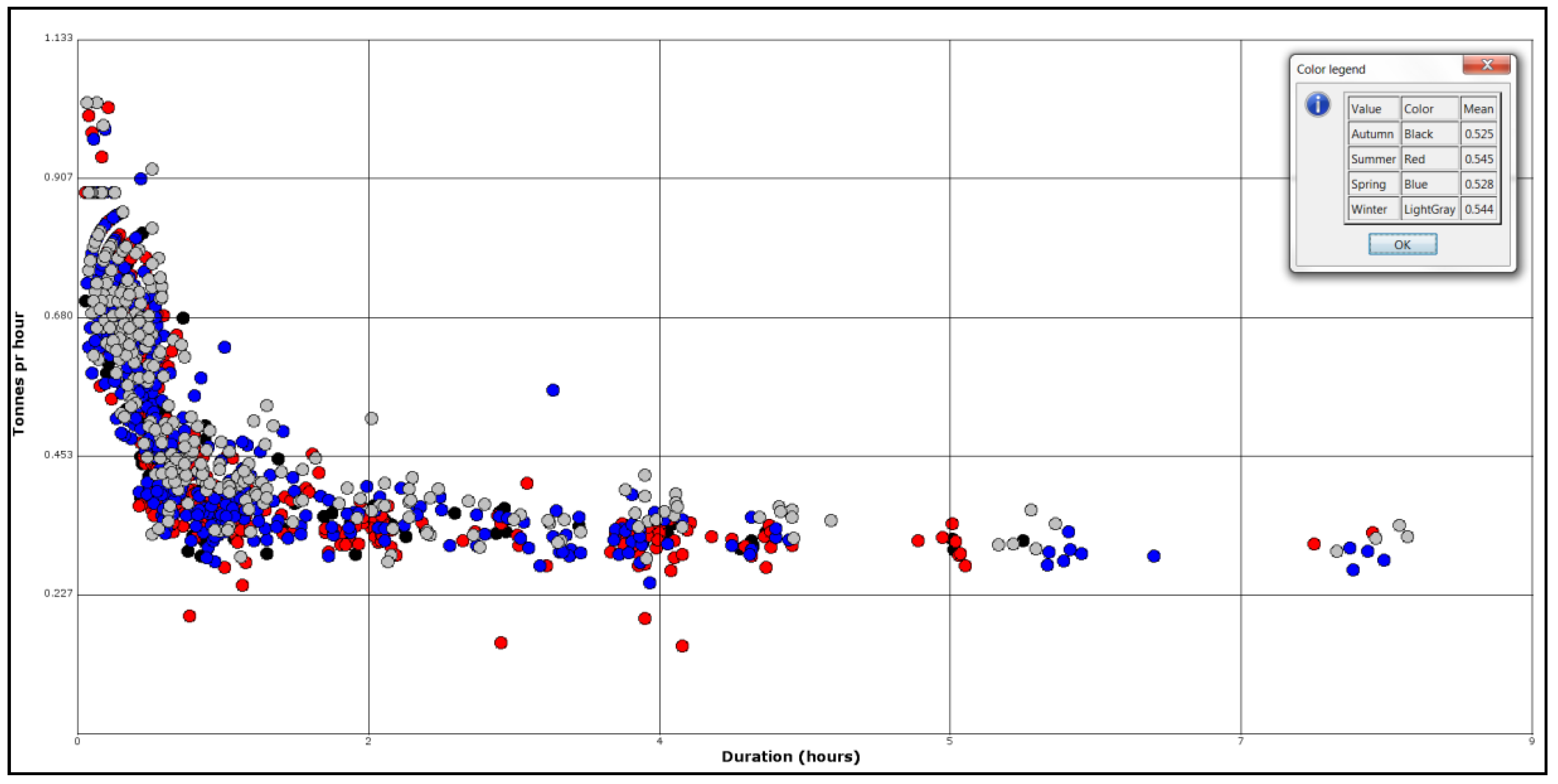
Figure 3 shows the relationship between duration of stay in port and fuel consumption in tons per hour. Hurtigruten AS registers fuel consumption in litre. We have converted to kg using a density of 0.883 kg per litre for medium speed diesel. A 12 h stay in the port of Rissa on 28 March 2017, is excluded because the ship was docked. We have also excluded a 4.12 h stay in Tromsø on 16 June 2017, where the recorded fuel consumption for the whole stay is only 26.5 kg, i.e., 6 kg per hour.

All in all we have 1520 registrations of stays in port with date, duration and fuel consumption for the Finnmarken. The estimated mean fuel consumption per hour is 536 kg and the mean power consumption is 2024 kWh.

Table 5. Energy consumption and specific fuel consumption for Finnmarken.

Percentile	kWh in Port	Tons of Fuel per hour in Port	kWh at Sea	kg of fuel per kWh at Sea
0	943	0.144	2403	0.199
0.05	1111	0.308	3833	0.208
0.10	1173	0.327	4026	0.209
0.25	1347	0.369	4251	0.212
0.50	1856	0.502	4516	0.215
0.75	2692	0.698	4843	0.219
0.90	3002	0.773	5162	0.223
0.95	3222	0.803	5530	0.226
1.00	4353	1.030	7958	0.375
Mean	2025	0.537	4575	0.217
CV	37.0	33.5	12.9	7.2

shows percentiles for energy consumption in port and at sea for Finnmarken. The median energy consumption in port is 1856 kWh, while 75% of registered stays in port have consumption values below 2700 kWh. Only 10% of stays in port have energy consumption values larger than 3000 kWh. The median specific fuel consumption is 0.215 kg per kWh at sea.

Table 5 shows Coefficient-of-variation (CV), which is the standard deviation in percentage of the mean. The larger the CV value, the larger is the variation of one distribution compared to another. As Table 5 shows, energy and fuel consumption in port vary more than energy consumption and specific fuel consumption at sea.

According to Figure 3 and Table 5, the longer the stay, the lower is the energy consumption per hour. This effect can be explained by the fact that energy use for a ship manoeuvring in port makes up a larger proportion of total energy use, the shorter the time it spends in port.

A log-log model is used to capture the relationship between port stay and fuel consumption in Figure 3. The model proposes that fuel consumption in tons per hour decreases with a constant percentage ratio for time spent in port. In addition to length of stay, time of year is considered, divided into winter, spring, autumn and summer. Winter is defined as months December, January and February, spring as March, April and May, summer as June, July and August and autumn as September, October and November. The three first seasons are represented with a dummy variable. There is one more season than dummy variables, therefore summer was represented by the intercept in the model. Regression model for fuel consumption in tons per hour in port is defined as follows:

$$\ln \left(\mathrm{Y}\right)={\mathsf{\beta }}_0+{\mathsf{\beta }}_1\left(\ln \left(\mathrm{Duration}\right)\right)+{\mathsf{\beta }}_2\mathrm{Winter}+{\mathsf{\beta }}_3\mathrm{Spring}+{\mathsf{\beta }}_4\mathrm{Autumn}+\mathsf{\epsilon }$$

(28)

The dependent variable, Y, is log of fuel consumption in tons per hour in port. All logs are based on the natural logarithm. The independent variables are defined in

Table 6. Definitions of independent variables in regression model for Finnmarken’s fuel consumption in port.

Variable Name	Explanation
Duration	Log of hours spent in port. The variable measures fraction of hours so that 5 min in port equals 0.083 h.
Winter	Dummy variable with value 1 for months December, January, and February.
Spring	Dummy variable with value 1 for months March, April, and May.
Autumn	Dummy variable with value 1 for months September, October, and November.

.

Based on estimation of the regression model fuel consumption in port the following coefficents were obtained:

$$\mathrm{Y}=-0.874-0.274\left(\mathrm{Duration}\right)+0.074\times \mathrm{Winter}-0.004\times \mathrm{Spring}-0.025\times \mathrm{Autumn}$$

(29)

The coefficient for duration shows that if the stay in port increases by 1 percent, the fuel consumption measured in tons per hour decreases by 0.27 percent.

These coefficients are in log form. To obtain predicted values in tons per hour we use the formula:

$$\hat{\mathrm{Y}}={\mathrm{e}}^{\left(-0.874-0.274\times \left(\ln \left(\mathrm{Duration}\right)\right)+0.074\times \mathrm{Winter}-0.004\times \mathrm{Spring}-0.025\times \mathrm{Autumn}\right)}$$

(30)

The intercept estimates mean fuel consumption in summer months which is:

$$\mathrm{Summer}={\mathrm{e}}^{\left(-0.874\right)}=0.417\mathrm{tons}\mathrm{per}\mathrm{hour}$$

(31)

The coefficient for winter is statistically significant (p < 0.05) which means that consumption in winter months is higher than in summer. The estimated fuel consumption in autumn is not significantly different from consumption in summer while the consumption in spring is statistically weak (p = 0.058).

These coefficients will be used to predict fuel consumption in port. Since Hurtigruta’s ships are small, use of this formula is restricted to cruise ships with less than 25,000 gross tons. Cruise ships over this limit also have different hotel functions. For these ships coefficients will be based on the Alaska study (above 70,000 gross tons) [46] or the Marintek study [47] as discussed above. Total fuel consumption in port is calculated by using estimated tons per hours from Equation (29) and then multiply with duration in hours calculated as a fractional variable.

For all cruise ships, it is assumed that fuel consumption for hotel functions at sea is identical to the consumption in port. A standard duration of one hour is defined for hotel functions at sea, excluding fuel consumption used for manoeuvring during shorter stays in port. This standard duration is used to find the estimated tons per hour and then multiply with actual duration to find total fuel consumption for hotel functions. The duration is measured as a fractional number allowing for durations of less than one hour.

2.7. Speed Filter

In some cases, the estimated nautical miles and the corresponding time span fit poorly with the recorded speed. This is especially true when the time span is more than the default 5 min and the assumption that the registered speed is the same for the whole time span is inappropriate. Therefore, if a time span exceeds 15 min it is set to a default of 5 min. An extra filter is applied to exclude high recorded speed values relative to calculated nautical miles. This filter, shown in Equation (32), calculates speed in knots based on the time span and estimated nautical miles based on latitude and longitude values. If this estimated speed is less than the cut-off value of 4 knots, it is assumed that the ship is in port or manoeuvring in port. Calculated speed filter is defined as follows:

$${\mathrm{Speed}}_{\mathrm{calculated}}=\frac{\left(\frac{{\mathrm{minutes}}_{\mathrm{time}-\mathrm{span}}}{60}\right)}{\mathrm{nautical}-\mathrm{miles}}$$

(32)

3. Model Validations

This part details as to whether the formula developed by IMO (see Equation (15)) is valid for cruise ships that sail to Norway. Real-world data from fuel monitoring of the data system on MS Finnmarken is used for this purpose. The data contains information about the start and end date for each route, distance sailed, average speed, fuel consumption in litre per nautical mile, and power production.

Fuel consumption data was also obtained for the cruise ship Artania for a round trip to the Arctic in June 2017. Data was provided by the chief machinist [50]. The ship travelled from Bremerhaven, Germany, to Reykjavik, Iceland. From Reykjavik, the ship travelled to the Norwegian communities of Longyearbyen and Spitsbergen in the Arctic Ocean, and then back to the Norwegian mainland where it visited Nordkapp, Tromsø, Geiranger, Bergen, and Lyngdal before returning to Bremerhaven. It must be noted that its total fuel consumption is not as well documented as for Finnmarken, where full documentation of the ship’s movements and fuel consumption on each travelled route was obtained. The Artania fuel consumption data must therefore be regarded as indicative and not as conclusive evidence of the ship’s fuel consumption.

We will also give estimates for the route travelled by the cruise ship Norwegian Star in May 2016, a ship which, measured in engine power and size, is considerably larger than Artania and Finnmarken. The model is therefore validated against cruise ships that vary in size and installed engine power. This validation allows us to reflect on the strengths and weaknesses of the model with respect to different speed profiles, ship sizes, and power plant set-up.

Table 7. Ships used in model validation.

Symbol	Property	Finnmarken	Artania	Norwegian Star
-	Year built	2002	1984	2001
-	Gross tons	15,690	44,656	91,740
-	Dead weight	945	4661	7500
-	Berths	643	1200	3000
-	Power installed (kW mcr)	13,800	29,160	58,800
-	Service speed (knots)	18	22	24.6
-	Max speed (knots)	-	-	26
-	Validation period	May 2017	June 2017	May 2016
A	Distance travelled (nautical miles)	7564.1	4381.5 #	2638.8 #
-	Fuel consumed (tons)		-	-
-	- At sea	525.9	-	-
-	- In port	62.5	-	-
B	Total	588.4	1050.8	-
C = B/A × 1000	kg per nautical mile	77.8	239.8	-

^# Estimated distances from AIS data.

shows characteristic attributes for the three ships.

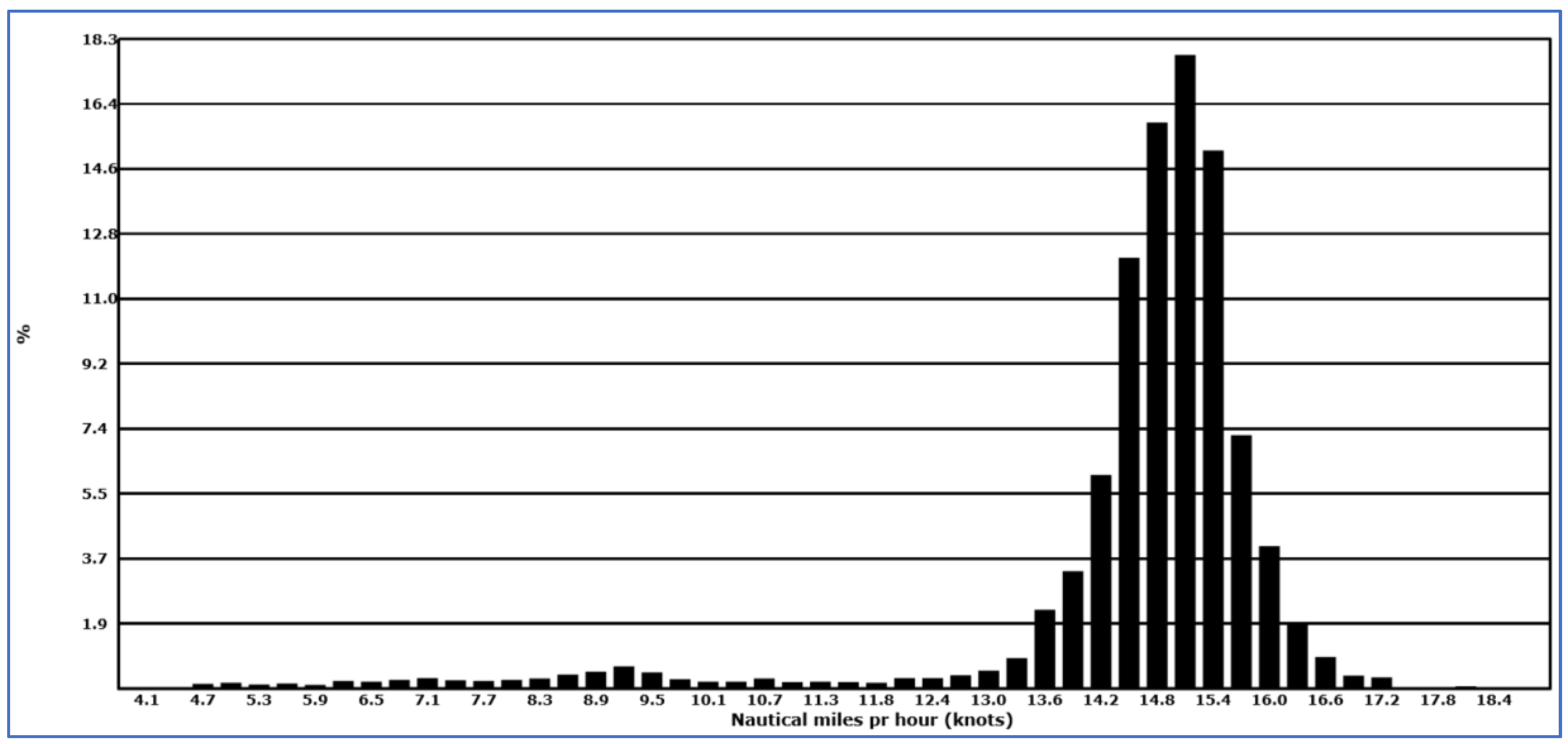
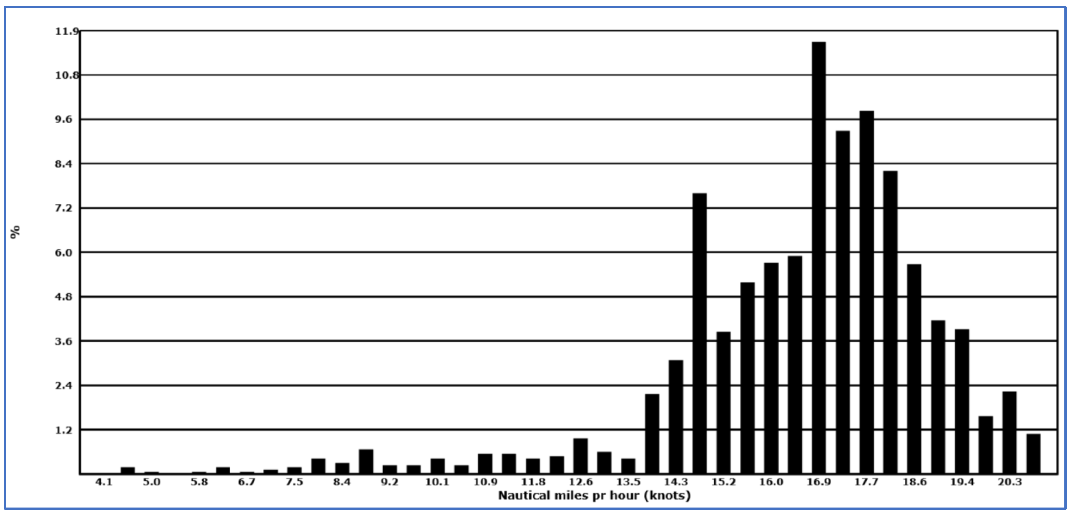
The three ships have quite different speed profiles, which will influence the estimates of total fuel consumption in the models presented here. Figure 4 shows the speed profile for Finnmarken in May 2017.

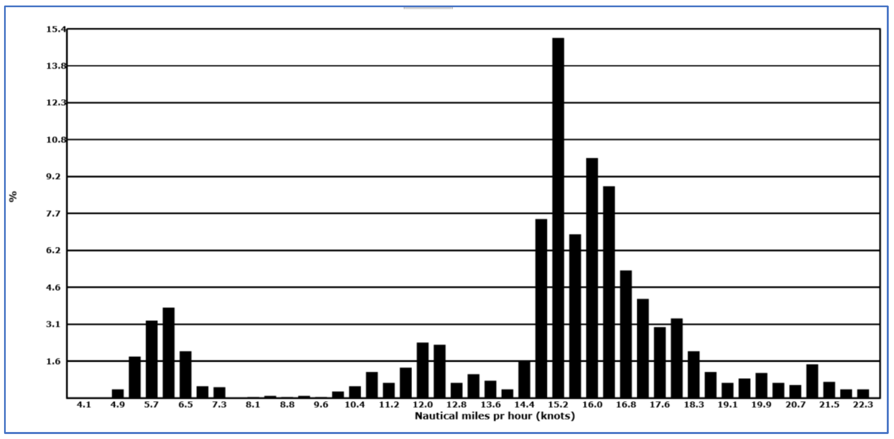
Figure 5 shows the same profile for Artania in June 2016, and Figure 6 shows the profile for Norwegian Star in May 2016. Finnmarken seems to have a much more pointed distribution with a thinner right tail than the other ships. Artania has a less pointed distribution with a much thicker right tail, while Norwegian Star falls in the middle with more variation in the left tail. This variation is probably due to sailing between Ålesund and Geiranger at night. Since the distance is short, the ship travels at lower speed to reach Geiranger in the morning.

Table 8. Percentiles and descriptive statistics for speed distributions.

Symbol	Ship	Finnmarken	Artania	Norwegian Star
-	Period	May 2017	June 2017	May 2016
-	Min	4.1	4.1	4.1
-	P5	8.8	11.1	5.6
-	P10	12.7	13.7	6.1
-	P25	14.3	15.1	14.2
-	P50	14.8	16.7	15.2
-	P75	15.3	17.9	16.4
-	P90	15.7	18.9	18
-	P95	16	19.5	20.5
-	Max	19	21.1	22.7
A	Mean	14.3	16.2	14.4
B	Standard deviation	2.1	2.6	3.9
B/A×100	CV	14.7	16.0	27.1

shows percentiles and descriptive statistics for the speed distributions of the three ships. Norwegian Star and Finnmarken have roughly the same mean speed even if the service speed for Norwegian Star is 24 knots and 18 knots for Finnmarken. Artania has a higher mean speed. Measured by the CV factor (coefficient-of-variation, standard deviation normalized to the mean in percentages), Norwegian Star has more variation in applied speed than the other two ships.

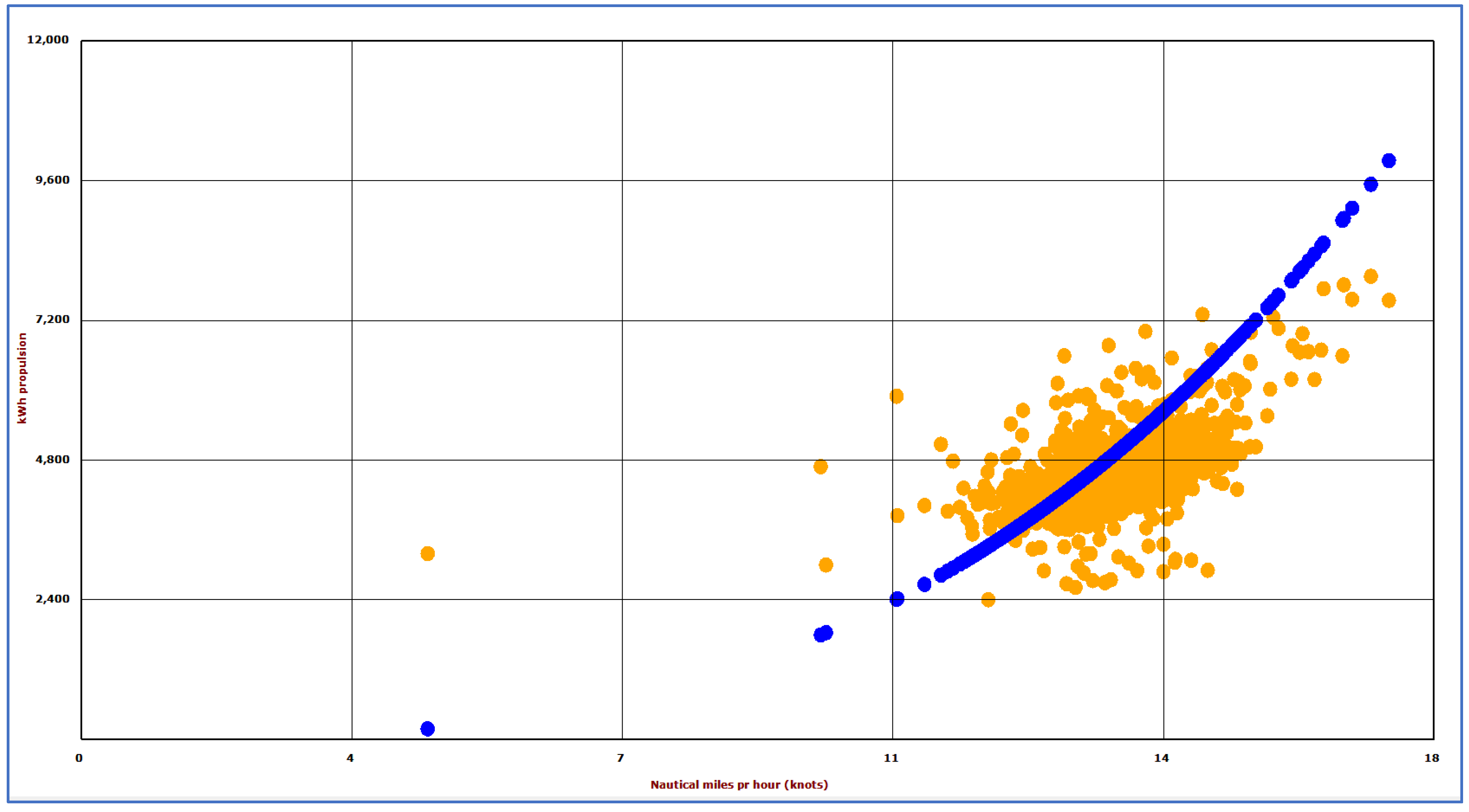
Figure 7 shows energy consumption for propulsion in kWh for Finnmarken in May 2017 for both real values (orange points) and estimated values (blue points) from the IMO formula Equation (12). For speeds above 16 knots, the IMO formula calculates energy consumption up to 2000 kWh greater than real values. The best fit between the models is at mid-range speed values or at about 14 knots (i.e., approximately 75% of the service speed). The higher and lower the speed is, the larger the deviation from the real-world values. For example, at speeds below 11 knots, the IMO values are up to 1500 kWh lower than the real-world Finnmarken values. The figure shows that IMO values vary much more than real values. The AIS data provided information about speed over ground; however, this speed is different than the speed through water [1]. The speed can vary at a constant engine load and propeller speed because of changes in environmental conditions such as waves, wind, and current [51].

Table 9. Estimates for validation period using IMO formula for load and specific fuel consumption.

Symbol	Property	Finnmarken	Artania	Norwegian Star
-	Month	May 2017	June 2017	May 2016
A	Nautical miles	7369.6	4381.5	2638.8
B	Duration at sea (hours)	535.9	300	184
B	Duration in port (hours)	213	80	92
-	Fuel consumption, tons	-	-	-
C	Propulsion	588.4	567.2	411
D	Hotel functions at sea	219.4	217.5	304.6
E	In port	77	65	152.7
F = D + E	Hotel function total	296.4	282.5	457.3
G = C + F	Total	884.8	849.7	868.3
H = G/A × 1000	kg pr nautical mile	120.1	193.9	329.1

shows estimated data for the three ships using the IMO formula for load (Equation (14)) (and specific fuel consumption (Equation (17)). This model will be referred to as Model A.

For Finnmarken, the model estimate for total fuel consumption is roughly 296 tons or 50% higher than the actual consumption. However, Finnmarken has a non-conventional drive train and during sailing, electric power is only retrieved from the shaft generators and thus the ship functions as a diesel-eletric ship (i.e., sharing the power between propulsion and hotel functions). Fuel consumption for hotel functions at sea are included when calculating total fuel consumption, thus assuming that the total MCR goes to propulsion. Including the hotel function at sea can lead to a bias since the estimated fuel consumption may be larger than what the total MCR allows for. Consequently, an upper limit for fuel consumption assuming a load factor of 1 in Equation (17) in introduced. If the total estimated fuel consumption is larger than this upper limit, fuel consumption for propulsion is calculated as the difference between the upper limit and the estimated fuel for hotel functions.

It can be argued that the hotel load at sea should be excluded from the calculations of non-conventional geared systems. If excluded, this leads to an overestimation of about 10.6% for the IMO-formula compared to the real-world values. For stays in port, the model estimate is 14.5 kg or 23% higher than the actual numbers for Finnmarken. Measured in kg per nautical mile, the model estimate is 42 kg or 54% higher than real values. If hotel functions at sea are excluded, the estimated fuel consumption is 13.1% higher than real values.

For Artania, the model estimate is 201 tons or 19% lower than the actual figure, using a service speed of 22 knots. The IMO model is sensitive to the observed speed relative to the service speed. Other variables such as draught (only minor differences observed for cruise ships), weather, and fouling are constants. It has been difficult to find the correct service speed for Artania. According to to the operator Phoenix Reisen [52], it is between 15–18 knots. Changing the service speed has a huge impact on the result from Equation (15). For a service speed of 18 knots, the model overestimates fuel consumption by 18.3%.

For Norwegian Star, the actual figure for total fuel consumption is unknown, but measured in kg per nautical mile, the estimate is close to 70% higher than values for Artania. For comparison, the Norwegian Star is twice the size of Artania measured in gross tons. For Norwegian Star, the estimated fuel consumption required for hotel functions at sea is 67% of the estimated fuel consumption for propulsion. The ship’s recorded speeds are low compared to the service speed and an average load factor of 0.28.

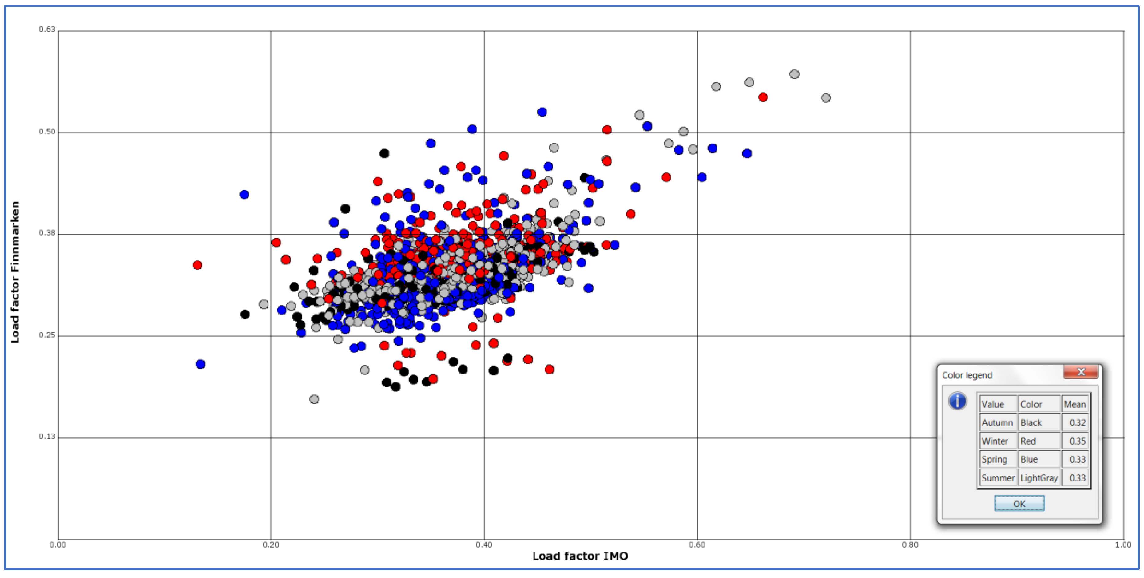
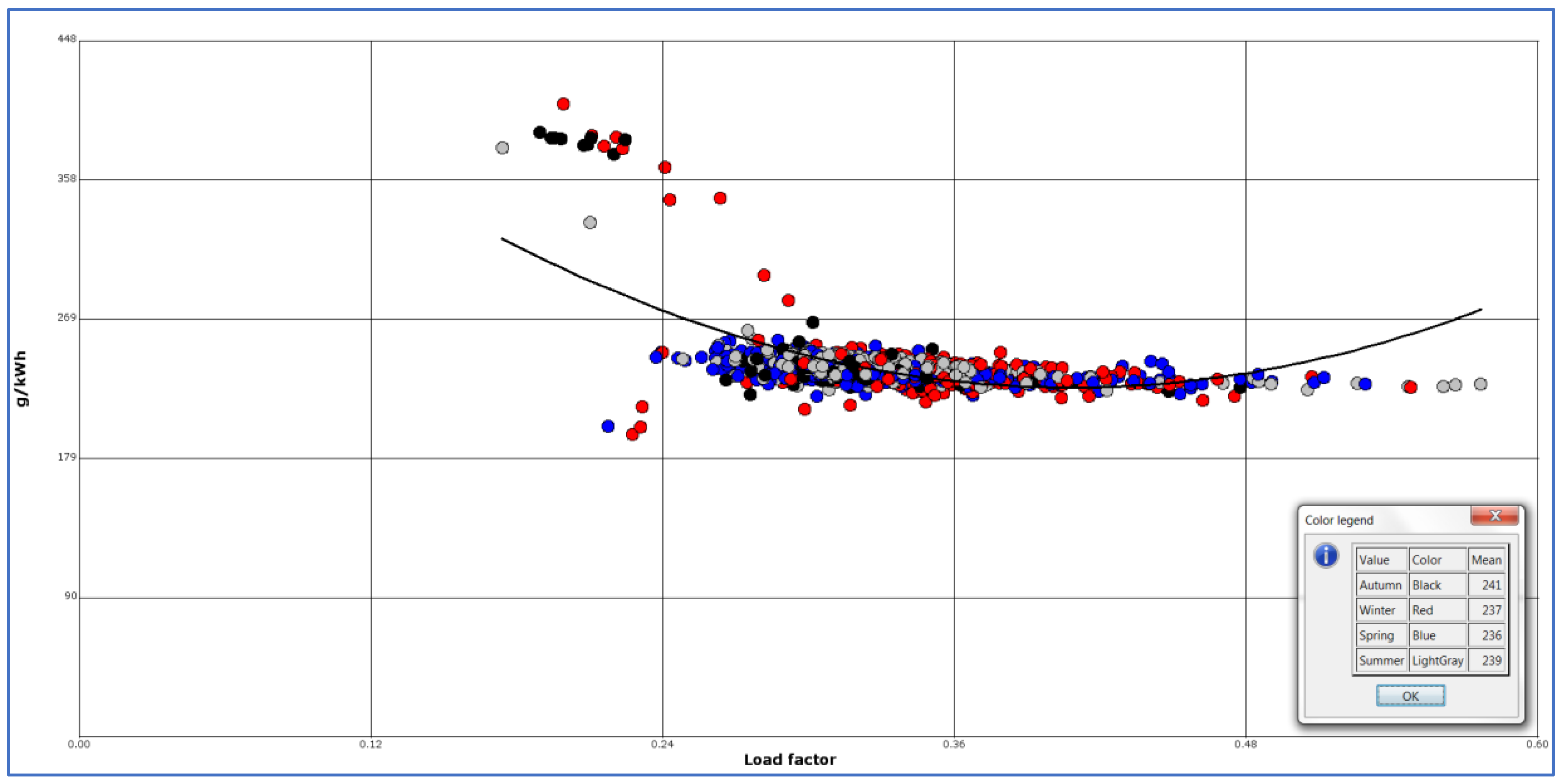
Figure 8 shows the load factor estimated with the IMO equation versus the actual load values for Finnmarken. The blue data points are registrations from the spring season, red are from the winter season, black from autumn, and light grey from summer.

A perfect fit between the two would imply that all data points should lie on a straight line. A linear regression line estimated on the points in Figure 8 give an R² of 0.31, which means that 31% of the variations in actual load from Finnmarken can be explained by the formula used by IMO. This may indicate that using load estimated from Finnmarken would give better model adaptions to real data.

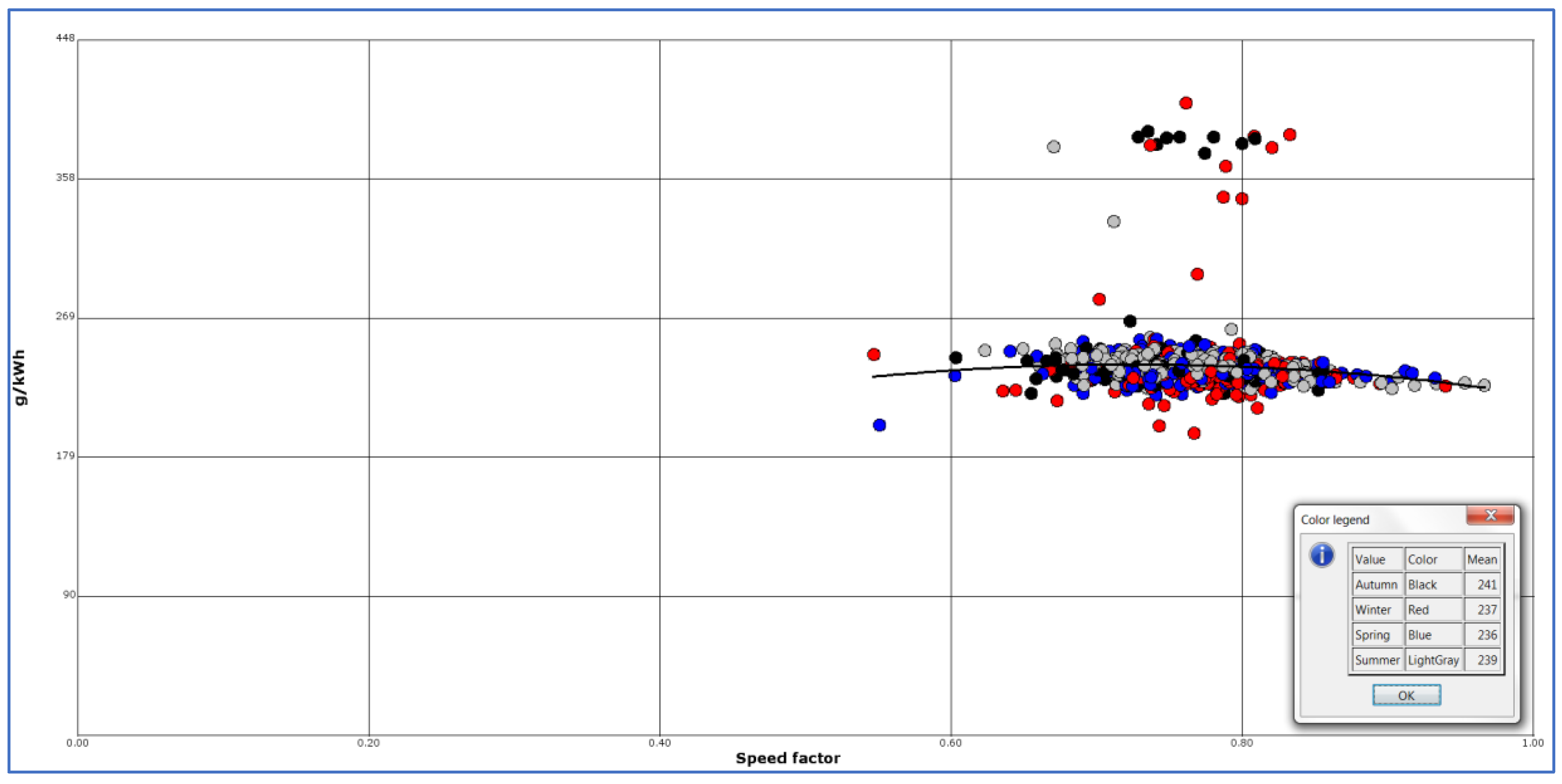
The speed factor used is defined as the actual speed divided by the service speed. The specific fuel consumption is calculated using the formula in Equation (17). This is referred to as Model B. Since hotel functions are included in the load factor for Finnmarken, a second-degree polynomial functional form for speed factor is assumed. This functional form reflects that load values will be higher for lower speeds since hotel functions vary independently of speed. We estimate load factor from Finnmarken data as follows:

$$\mathrm{Y}={\mathsf{\beta }}_0+{\mathsf{\beta }}_1\times \mathrm{SpeedFactor}+{\mathsf{\beta }}_2\times {\mathrm{SpeedFactor}}^2+{\mathsf{\beta }}_2\times \mathrm{Winter}+{\mathsf{\beta }}_3\times \mathrm{Spring}+{\mathsf{\beta }}_4\times \mathrm{Autumn}+\mathsf{\epsilon }$$

(33)

Estimation of that equation gives the coefficients in

Table 10. Estimated coefficients for estimating load factor from Finnmarken data.

Symbol	Value
b0	1.771
b1	−4.274
b2	3.109
b3	0.017
b4	0.002
b5	−0.006

. The estimated b-coefficients in Table 10 correspond to population parameters $\mathsf{\beta }$ in Equation (33).

Table 11. Estimates for validation period with load estimates from Finnmarken data and specific fuel consumption from IMO.

Symbol	Property	Finnmarken	Artania	Norwegian Star
-	Month	May 2017	June 2017	May 2016
A	Nautical miles	7369.6	4381.5	2638.8
-	Fuel consumption, tons	-	-	-
C	Propulsion	476	580.4	585.7
D	Hotel functions at sea	0	0	304.6
E	In port	77	65	152.7
F = D + E	Hotel function total	77	65	255.2
G = C + F	Total	553	645.5	1043
H = G/A × 1000	kg per nautical mile	75	147.3	395.3

shows model estimates with the load factor estimated from Finnmarken data.

The minimum speed value used to calculate the coefficients in Equation (33) is 9 knots. This speed yields a speed factor of roughly 0.5 with a service speed of 18 knots. The estimated load is 0.43, assuming the speed is recorded in winter months. If we use speed values less than 9 knots, calculate speed factor, and then apply Equation (33), we will get higher load values the less the actual speed is. If the speed is equal to 6 knots, the speed factor will be 0.36 and the estimated load value 0.65. If the speed is equal to 5 knots, the speed factor will be 0.28 and the estimated load value 0.77. This is clearly an extrapolation problem; we estimate load factors for speed factors far less than those we used to estimate coefficients in Equation (33). To overcome this problem, we will apply a floor value of 7 knots. This speed gives a load value of 0.59. Speed values below that floor value will be set equal to the floor value. This will mostly apply to speed values for manoeuvring in port and will have less impact on the total fuel consumption.

Using this approach, we do not calculate fuel consumption for hotel functions at sea for Finnmarken or Artania. This fuel consumption is embedded in the estimated load factor for these ships since they are not diesel-electric. For Norwegian Star, we include hotel functions at sea since it is a diesel-electric ship where auxiliary engines provide power for both propulsion and hotel functions.

The results from using this model are presented in Table 11. It shows that the estimated total fuel consumption for Finnmarken is almost 36 tons or 6% lower than the actual figure. The estimate in kg per nautical mile is 2.8 kg or 3.6% lower than the actual figure. For Artania, the total fuel consumption is 405 tons or almost 39% lower than the actual figure. The total fuel estimate for Norwegian Star is 175 tons higher compared to the value obtained from using the IMO formula for load calculations. The load model based on Finnmarken data assume relatively high load at low speeds compared to the IMO formula. This difference suggests that the formula based on Finnmarken data should not be used for ships with similar speed profile as Norwegian Star.

Finally, we look at the results from a two-stage model, where both load and specific fuel consumption (sfc) were estimated using Finnmarken data. In the first stage, the estimated load factor is still based on Equation (33). In the second stage, the specific fuel consumption is estimated from Finnmarken data using Equation (34) instead of using the IMO formula in Equation (17). The estimated load factor from stage 1 is used as input for estimating specific fuel consumption in stage 2. This model design means that speed factor has a direct effect on fuel consumption as well as an indirect effect through estimation of load values. This will be referred to as Model C. As mentioned above, a second-degree polynomial functional form is assumed for speed factors since load and fuel consumption for hotel functions are independent of speed. This implies that load and specific fuel consumption will be higher for lower speed values.

Figure 9 shows the relationship between specific fuel consumption and load factor from Finnmarken. The estimated trend in the figure gives an R² of 0.389. Figure 9 shows the relationship between speed factor and specific fuel consumption from Finnmarken.

Figure 10 shows the relationship between specific fuel consumption and speed factor from Finnmarken. Speed factor is defined as actual speed in nautical miles pr hour over design speed.

The specific fuel consumption factor from Finnmarken data is estimated as follows:

$$\mathrm{Y}={\mathsf{\beta }}_0+{\mathsf{\beta }}_1\times \mathrm{SpeedFactor}+{\mathsf{\beta }}_2\times {\mathrm{SpeedFactor}}^2+{\mathsf{\beta }}_3\times \mathrm{LoadFactor}+\mathsf{\beta }\times {\mathrm{LoadFactor}}^2+{\mathsf{\beta }}_5\times \mathrm{Winter}+{\mathsf{\beta }}_6\times \mathrm{Spring}+{\mathsf{\beta }}_7\times \mathrm{Autumn}$$

(34)

The estimated regression coefficients from Equation (34) are shown in

Table 12. Coefficients for estimating specific fuel consumption from Finnmarken data.

Symbol	Value
b0	179.0568
b1	882.0727
b2	−550.886
b3	−1602.37
b4	1954.498
b5	4.464916
b6	−3.44262
b7	−0.90836

. The results of applying this model on the three ships are shown in

Table 13. Estimates for validation period with load and specific fuel consumption estimated from Finnmarken data.

Symbol	Property	Finnmarken	Artania	Norwegian Star
-	Month	May 2017	June 2017	May 2016
A	Nautical miles	7369.6	4381.5	2638.8
-	Fuel consumption, tons	-	-	-
C	Propulsion	490.7	593.3	896
D	Hotel functions at sea	0	0	304.6
E	In port	77	65	152.7
F = D + E	Hotel function total	77	65	457.3
G = C + F	Total	567.7	658.4	1353.3
H = G/A × 1000	kg per nautical mile	77	150.3	512.8

.

The main difference between the new model in Table 13 and the previous model in Table 11 is that Finnmarken estimates are now closer to the observed values. The estimate for total fuel consumption is 21 tons or 3.5% lower than the actual figure, while the estimate for kg per nautical mile is 0.8 kg or 1% off target. The estimated figure for total fuel consumption for Artania is 392 tons or 37% lower than the actual one.

The estimated total fuel consumption increases for all three ships compared to the previous model. The increase is largest for Norwegian Star (310 tons) and lowest for Artania (13 tons).

Table 14. Estimates for total fuel consumption for Finnmarken, Artania, and Norwegian Star with different models.

Total	Nautical Miles	Model A IMO Formulas	Model B Load from Finnmarken, sfc # from IMO	Model C Load and sfc from Finnmarken
Finnmarken	7369.6	884.8	553	567.7
Artania	4381.5	849.7	645.5	658.4
Norwegian Star	2638.8	868.3	1043	1353.3

^# Specific fuel consumption, g/kWh.

shows total fuel consumption estimates for the three ships used in the analysis. In model C, fuel consumption for Artania goes down while it increases for Norwegian Star. If the service speed for Artania is set to 18 knots in Model C, total fuel consumption is estimated to amount to 1088 tons, which is 3.4% higher than observed values. This shows how sensitive the estimates are for variations in service speed in the model.

Since Norwegian Star is a diesel-electric cruise ship, fuel consumption for hotel functions is added to total fuel counsumption in Model C. This is also reflected in

Table 15. Estimates for kg pr nautical mile for Finnmarken, Artania, and Norwegian Star with different models.

Total	Nautical Miles	Model A IMO Formulas	Model B Load from Finnmarken, sfc from IMO	Model C Load and sfc from Finnmarken
Finnmarken	7369.6	120.1	75.0	77
Artania	4381.5	193.9	147.3	150.3
Norwegian Star	2638.8	329.1	395.3	512.8

, which illustrates kg of fuel use per nautical mile for the different ships with the different models.

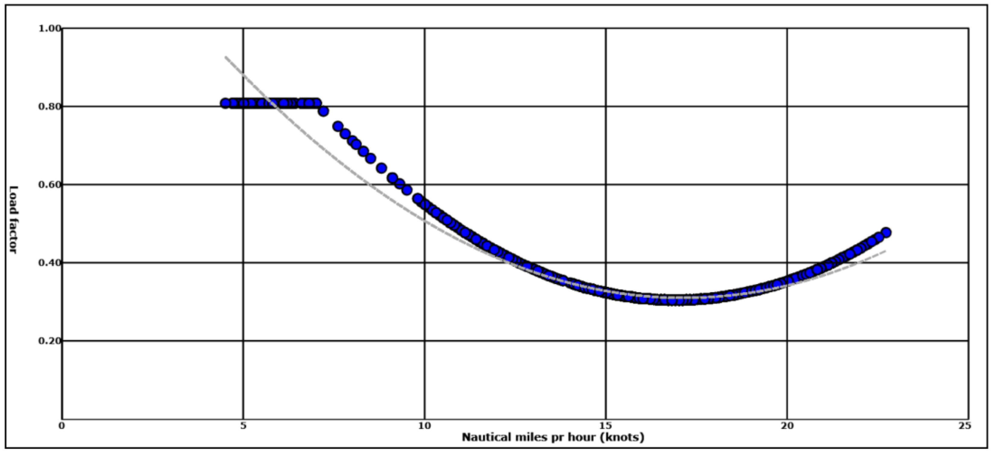
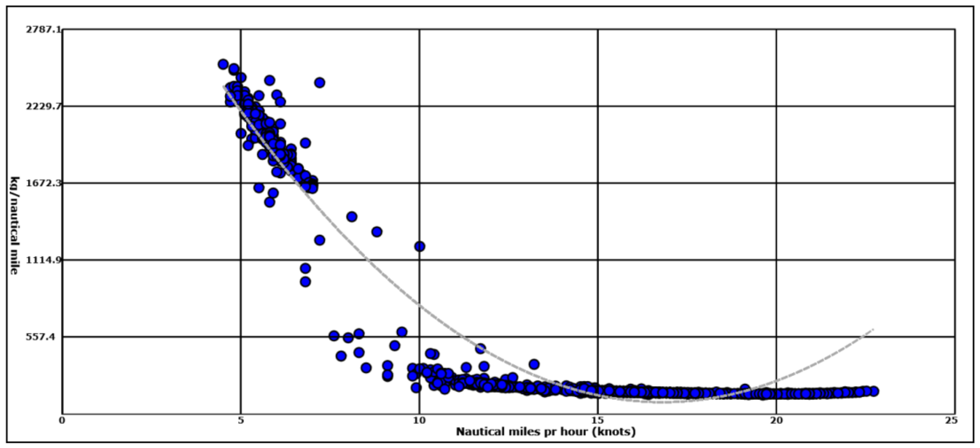
Figure 11 shows the load profile for Norwegian Star in May 2016 using Finnmarken data for both load factor and specific fuel consumption. As can be seen in the figure, a floor value for speeds has been applied below 7 knots as described above. Figure 12 shows the propulsion profile for the same ship in the same month using Finnmarken data. In Figure 13 and Figure 14, the same profiles are shown using IMO formulas. It is obvious that the profile is totally different for Norwegian Star using Finnmarken data. For lower speeds, the estimates based on Finnmarken data will give higher loads and higher fuel consumption per nautical mile; while for higher speeds, the pattern is the opposite—IMO formulas will give higher consumption per nautical mile.

4. Discussion

Models B and C have been designed using data from the smaller cruise ship Finnmarken. These models are used to estimate load values and fuel consumption for larger cruise ships such as Norwegian Star. In both models, a-degree polynomial functional form for the independent variable speed factor has been assumed. This functional form reflects that load and fuel consumption for hotel functions vary independent of speed. A problem with this approach is that Norwegian Star has a diesel-electric engine configuration, and hotel functions are not embedded in the estimated load values for this ship. Models B and C therefore do not fit well with the ship’s design.

Also, fuel consumption for hotel functions is far larger for Norwegian Star than for the other two ships. If we look at Model A, using IMO formulas, fuel for hotel functions makes up 20.5% of total fuel for propulsion for Finnmarken, while the corresponding figure for Norwegian Star is 74%. A main explanation for this difference is the speed distribution—Norwegian Star spends a lot of time at lower speeds. As a result, the share of fuel consumption for hotel functions become comparably larger than for Finnmarken. Models B and C should consequently not be used on diesel-electric ships where fuel consumption values for propulsion and hotel functions have been separated. These ships should use Model A based on the IMO formula for load values and specific fuel consumption.

If we look at Models B and C, estimates for total fuel consumption for Finnmarken and Artania fit better with estimates for propulsion in Model A than with estimates for total fuel consumption in the same model. Total fuel consumption includes hotel functions, and these functions can be included twice for Finnmarken and Artania in Model A by using total available power (MCR) in the calculation of load values and then also add hotel functions.

Artania and Finnmarken have quite different hotel functions. Finnmarken [53] has a swimming pool and whirlpool on deck, a cafe, a restaurant, a library, and a boutique. Artania [54] has three restaurants, seven bars, one library, one whirlpool, two outdoor swimming pools, one cinema, and a show lounge. As a consequence, it is not reasonable to expect that the load values estimated in Model B and C, based on Finnmarken data, will cover all hotel functions for Artania. It is therefore suggested that Model A should be used for ships above 25,000 gross tons since these ships can be expected to have more extensive hotel functions than Finnmarken. Also, for these ships, a cubic relationship between speed and load values as specified in Model A can be expected.

The two-step regression approach in Model C should be used for ships with tonnage below 25,000 gross tons and with a comparable sailing pattern. However, care should be taken when these ships spend a lot of time at lower speed.

All models are sensitive to the ratio of actual speed to service speed. An incorrect service speed will have a large impact on model estimates. Also, Model A requires a clear distinction between fuel consumption for propulsion and hotel functions. This distinction is readily available for diesel-electric ships since the proportion of total installed power that is associated with propulsion is known. For geared systems, this distinction is harder to make. Total fuel consumption for these ships may be overestimated if all engine power (in MCR) is applied to propulsion and hotel functions are added. Model validations show that fuel consumption for hotel functions at sea contribute a significant amount to total fuel consumption for cruise ships.

IMO’s third GHG study suggests that total cruise ship fuel consumption was 11.1 Mt in 2012 (main and auxiliary engines), corresponding to CO₂ emissions of 34.9 Mt [1]. In comparison, Carnival Corporation and Royal Caribbean Cruises (RCL), which account for around 70% of global capacity and passenger volumes [55], reported emissions of 14.8 Mt CO₂ for 2012 [56,57].

A more accurate perspective on the importance of the cruise sector is emissions per capita and day. A sector’s contribution to climate change can appear negligible when considering its absolute contribution; yet, emissions are a function of individual actions, and per capita emissions have been the focus of policy negotiations in the past (cf. United Nations Framework Convention on Climate Change (UNFCCC)). With 20.9 million cruise passengers in 2012 [58], the IMO estimate (34.9 Mt CO₂) results in average emissions of 1671 kg CO₂ per person and cruise trip. This is significantly more than the 1200–1300 kg estimated by Eijgelaar [11] or Carnival’s 1067 kg CO₂ (considering 10.5 Mt of fuel and 9.8 Mio passengers). Assuming a worldwide average of 7 days for a cruise (slightly shorter for North Americans and longer for Europeans; [59]), passenger per day emissions would amount to around 239 kg CO₂ on the basis of IMO data [1]. However, a reason for the comparatively high figure in the IMO study could be that auxiliary engines have been added for both diesel electric and “geared systems” without subtracting it from total MCR, which, as this paper shows, could lead to an overestimation of fuel consumption on the order of 50%. Ships included in this paper are in the lower end of previous estimations of CO₂ emissions from cruise ships. A comparison between the ships is based on a marine fuel oil CO₂ emission factor of 3.114 [1]. MS Finnmarken emits 91.9 kg CO₂ per passenger day based on a pax number of 643 (Table 7). MS Finnmarken also transports freight, and a share of the emissions should be allocated to freight. Allocating one of eight decks to freight, the figure is 80.4 kg CO₂ per passenger. For Artania, which sails for 18 days in June 2017, the figure is 151.5 kg CO₂ per passenger day assuming a pax number of 1200 [60]; while for Norwegian Star, sailing for 11 days and 8 h in Norwegian waters in May 2016, it is 111.6 kg CO₂ per passenger day assuming a pax number of 2139 [61].

As pressure on the sector to reduce emissions grows, and as new market-based regulations [3] are introduced and imposed on the sector, the need for refined modelling capabilities is warranted. National authorities, as well as cruise operators, require such models in order to assess fuel consumption and emissions from cruise itineraries. Legal entities such as countries or municipalities require them to define policies. Models (see Supplementary Materials), such as the one presented in the article [62], are also easier to use than complex bottom-up assessments [26], and they can be used to project the outcome of operational changes or assess the impact of policy measures such as shore-side electricity in ports. The model validation shows the importance of having accurate information about ship sizes; ship design, allocation between propulsion and non-propulsion activities and in-depth knowledge about sailing patterns. This information, combined with well-designed models, is important in order to find most efficient policies for reducing fuel consumption and emissions from cruise travelling.

References

- Smith, T.; Jalkanen, J.; Anderson, B.A.; Corbett, J.J.; Faber, J.; Hanayama, S.; O’Keeffe, E.; Parker, S.; Johansson, L.; Aldous, L.; et al. Third IMO GHG Study 2014; International Maritime Organization: London, UK, 2014. [Google Scholar]
- Johansson, L.; Jalkanen, J.-P.; Kukkonen, J. Global Assessment of Shipping Emissions in 2015 on a High Spatial and Temporal Resolution. Atmos. Environ. 2017, 167, 403–415. [Google Scholar] [CrossRef]
- Shi, Y. Reducing Greenhouse Gas Emissions from International Shipping: Is It Time to Consider Market-based Measures? Mar. Policy 2016, 64, 123–134. [Google Scholar] [CrossRef]
- Mander, S.; Walsh, C.; Gilbert, P.; Traut, M.; Bows, A. Decarbonizing the UK Energy System and the Implications for UK Shipping. Carbon Manag. 2012, 3, 601–614. [Google Scholar] [CrossRef]
- Sharmina, M.; McGlade, C.; Gilbert, P.; Larkin, A. Global Energy Scenarios and Their Implications for Future Shipped Trade. Mar. Policy 2017, 84, 12–21. [Google Scholar] [CrossRef]
- Capaldo, K.; Corbett, J.J.; Kasibhatla, P.; Fischbeck, P.; Pandis, S.N. Effects of Ship Emissions on Sulphur Cycling and Radiative Climate Forcing over the Ocean. Nature 1999, 400, 743. [Google Scholar] [CrossRef]
- Corbett, J.J.; Winebrake, J.J.; Green, E.H.; Kasibhatla, P.; Eyring, V.; Lauer, A. Mortality from Ship Emissions: A Global Assessment. Environ. Sci. Technol. 2007, 41, 8512–8518. [Google Scholar] [CrossRef] [PubMed]
- Marelle, L.; Thomas, J.L.; Raut, J.-C.; Law, K.S.; Jalkanen, J.-P.; Johansson, L.; Roiger, A.; Schlager, H.; Kim, J.; Reiter, A.; et al. Air Quality and Radiative Impacts of Arctic Shipping Emissions in the Summertime in Northern Norway: From the Local to the Regional Scale. Atmos. Chem. Phys. 2016, 16, 2359–2379. [Google Scholar] [CrossRef] [Green Version]
- CLIA. About the Industry. Available online: https://www.cruising.org/about-the-industry/press-room/press-releases/cruise-lines-international-association-releases-official-2015-global-passenger-numbers-and-increases-2016-projections (accessed on 17 April 2018).
- Cruise Market Watch. Growth of the Ocean Cruise Line Industry. 2017. Available online: https://www.cruisemarketwatch.com/growth/ (accessed on 17 April 2018).
- Eijgelaar, E.; Thaper, C.; Peeters, P. Antarctic Cruise Tourism: The Paradoxes of Ambassadorship, “Last Chance Tourism” and Greenhouse Gas Emissions. J. Sustain. Tour. 2010, 18, 337–354. [Google Scholar] [CrossRef]
- Bonilla-Priego, M.J.; Font, X.; Pacheco-Olivares, M.D.R. Corporate Sustainability Reporting Index and Baseline Data for the Cruise Industry. Tour. Manag. 2014, 44, 149–160. [Google Scholar] [CrossRef]
- Butt, N. The Impact of Cruise Ship Generated Waste on Home Ports and Ports of Call: A Study of Southampton. Mar. Policy 2007, 31, 591–598. [Google Scholar] [CrossRef]
- Hall, C.M.; Wood, H.; Wilson, S. Environmental reporting in the cruise industry. In Cruise Ship Tourism, 2nd ed.; Dowling, R., Weeden, C., Eds.; CABI: Oxfordshire, UK, 2017; pp. 441–464. ISBN 978-178-064-608-4. [Google Scholar]
- Hritz, N.; Cecil, A.K. Investigating the Sustainability of Cruise Tourism: A Case Study of Key West. J. Sustain. Tour. 2008, 16, 168–181. [Google Scholar] [CrossRef]
- Klein, R.A. Cruise Ship Blues: The Underside of the Cruise Ship Industry, 2nd ed.; New Society Publishers: Gabriola Island, BC, Canada, 2002. [Google Scholar]
- Bows-Larkin, A. All Adrift: Aviation, Shipping, and Climate Change Policy. Clim. Policy 2015, 15, 681–702. [Google Scholar] [CrossRef]
- Johnson, D. Environmentally Sustainable Cruise Tourism: A Reality Check. Mar. Policy 2002, 26, 261–270. [Google Scholar] [CrossRef]
- Council of the European Union, European Parliament. Regulation (EU) 2015/757 of the European Parliament and of the Council of 29 April 2015 on the Monitoring, Reporting and Verification of Carbon Dioxide Emissions from Maritime Transport, and Amending Directive 2009/16/EC; Official Journal of the European Union: Brussels, Belgium, 2015. Available online: https://www.dnvgl.com/Images/2015_757_consolText_2016_2071_tcm8-86131.pdf (accessed on 22 April 2018).
- Matthias, V.; Aulinger, A.; Backes, A.; Bieser, J.; Geyer, B.; Quante, M.; Zeretzke, M. The Impact of Shipping Emissions on Air pollution in the Greater North Sea Region–Part 2: Scenarios for 2030. Atmos. Chem. Phys. 2016, 16, 759–776. [Google Scholar] [CrossRef]
- Rahim, M.M.; Islam, M.T.; Kuruppu, S. Regulating Global Shipping Corporations’ Accountability for Reducing Greenhouse Gas Emissions in the Seas. Mar. Policy 2016, 69, 159–170. [Google Scholar] [CrossRef]
- Gilbert, P.; Bows-Larkin, A.; Mander, S.; Walsh, C. Technologies for the High Seas: Meeting the Climate Challenge. Carbon Manag. 2014, 5, 447–461. [Google Scholar] [CrossRef]
- Yuan, J.; Ng, S.H.; Sou, W.S. Uncertainty Quantification of CO2 Emission Reduction for Maritime Shipping. Energy Policy 2016, 88, 113–130. [Google Scholar] [CrossRef]
- Corbett, J.J.; Wang, H.; Winebrake, J.J. The Effectiveness and Costs of Speed Reductions on Emissions from International Shipping. Transp. Res. Part D Transp. Environ. 2009, 14, 593–598. [Google Scholar] [CrossRef]
- CLIA. Environmental Technologies & Practices; CLIA Oceangoing Cruise Lines: Washington, DC, USA, 2017. Available online: https://cruising.org/docs/default.../environmental-technologies-and-practices-9-13.pdf (accessed on 22 April 2018).
- López-Aparicio, S.; Tønnesen, D.; Neilson, H. Shipping Emissions in a Nordic Port: Assessment of Mitigation Strategies. Transp. Res. Part D Transp. Environ. 2017, 53, 205–216. [Google Scholar] [CrossRef]
- Maragkogianni, A.; Papaefthimiou, S.; Zopounidis, C. Mitigating Shipping Emissions in European Ports; Springer International Publishing: Cham, Switzerland, 2016. [Google Scholar]
- Moreno-Gutiérrez, J.; Calderay, F.; Saborido, N.; Boile, M.; Valero, R.R.; Durán-Grados, V. Methodologies for Estimating Shipping Emissions and Energy Consumption: A Comparative Analysis of Current Methods. Energy 2015, 86, 603–616. [Google Scholar] [CrossRef]
- Hulskotte, J.; van der Gon, H.D. Fuel Consumption and Associated Emissions from Seagoing Ships at Berth Derived from an On-board Survey. Atmos. Environ. 2010, 44, 1229–1236. [Google Scholar] [CrossRef]
- Ritchie, A.; de Jonge, E.; Hugi, C.; Cooper, D. Report: Service Contract on Ship Emissions; ENTEC UK Ltd.: London, UK, 2005. [Google Scholar]
- Jalkanen, J.-P.; Brink, A.; Kalli, J.; Pettersson, H.; Kukkonen, J.; Stipa, T. A Modelling System for the Exhaust Emissions of Marine Traffic and Its Application in the Baltic Sea Area. Atmos. Chem. Phys. 2009, 9, 9209–9223. [Google Scholar] [CrossRef]
- EPA. Analysis of Commercial Marine Vessels Emissions and Fuel Consumption Data; U.S. Environmental Protection Agency: Washington, DC, USA, 2000.
- Corbett, J.J.; Koehler, H.W. Updated Emissions from Ocean Shipping. J. Geophys. Res. Atmos. 2003, 108. [Google Scholar] [CrossRef]
- Eyring, V.; Köhler, H.; Van Aardenne, J.; Lauer, A. Emissions from International Shipping: 1. The Last 50 Years. J. Geophys. Res. Atmos. 2005, 110. [Google Scholar] [CrossRef]
- International Maritime Organisation (IMO). Designation of an Emission Control Area for Nitrogen Oxides. Sulphur Oxides and Particulate Matter; Interpretations of and Amendments to MARPOL and Related Instruments 61st Session; IMO, Marine Environment Protection Committee: London, UK, 2010. [Google Scholar]
- International Maritime Organisation (IMO). Prevention of Air Pollution from Ships; International Maritime Organization: London, UK, 2010. [Google Scholar]
- Jalkanen, J.-P.; Johansson, L.; Kukkonen, J. A Comprehensive Inventory of Ship Traffic Exhaust Emissions in the European Sea Areas in 2011. Atmos. Chem. Phys. 2016, 16, 71–84. [Google Scholar] [CrossRef]
- Ng, S.K.; Loh, C.; Lin, C.; Booth, V.; Chan, J.W.; Yip, A.C.; Li, Y.; Lau, A.K. Policy Change Driven by an AIS-assisted Marine Emission Inventory in Hong Kong and the Pearl River Delta. Atmos. Environ. 2013, 76, 102–112. [Google Scholar] [CrossRef]
- Johansson, L.; Jalkanen, J.-P.; Kalli, J.; Kukkonen, J. The Evolution of Shipping Emissions and the Costs of Regulation Changes in the Northern EU Area. Atmos. Chem. Phys. 2013, 13, 11375–11389. [Google Scholar] [CrossRef]
- Goldsworthy, L.; Goldsworthy, B. Modelling of Ship Engine Exhaust Emissions in Ports and Extensive Coastal Waters Based on Terrestrial AIS Data–An Australian Case Study. Environ. Model. Softw. 2015, 63, 45–60. [Google Scholar] [CrossRef]
- Aulinger, A.; Matthias, V.; Zeretzke, M.; Bieser, J.; Quante, M.; Backes, A. The Impact of Shipping Emissions on Air Pollution in the Greater North Sea Region–Part 1: Current Emissions and Concentrations. Atmos. Chem. Phys. 2016, 16, 739–758. [Google Scholar] [CrossRef]
- Howitt, O.J.; Revol, V.G.; Smith, I.J.; Rodger, C.J. Carbon Emissions from International Cruise Ship Passengers’ Travel to and from New Zealand. Energy Policy 2010, 38, 2552–2560. [Google Scholar] [CrossRef]
- Calculate Distance, Bearing and More between Latitude/Longitude Points. Available online: http://www.movable-type.co.uk/scripts/latlong.html (accessed on 21 March 2018).
- Smith, T.; University College London, U.K. Personal communication, June 2017.
- AIS Class a Ship Static and Voyage Related Data (Message 5). Available online: https://www.navcen.uscg.gov/?pageName=AISMessagesAStatic (accessed on 15 April 2018).
- Graw, R.; Faure, A. Air Pollution Emission Inventory for 2008 Tourism Season Klondike Gold Rush National Heritage Park Skagway, Alaska; National Park Service: Washington, DC, USA, 2010.
- Stenersen, D. Operasjonsdata fra Skipsfart i Geiranger, Nærøy-og Aurlandsfjorden. Datainnsamling fra Cruiseskip og Lokal Trafikk; 302002020-1; SINTEF Norsk Marinteknisk Forskningsinstitutt AS: Trondheim, Norway, 2017; p. 41. [Google Scholar]
- Walle, O.C.; Hurtigruten AS. Personal communication, February 2018.
- Solberg, A.; JJ Ugland. Personal communication, February 2018.
- Sachse, B.V.; Norwegian National Broadcasting. Personal communication, September 2017.
- Marty, P.; Corrignan, P.; Gondet, A.; Chenouard, R.; Hétet, J.-F. Modelling of Energy Flows and Fuel Consumption on Board Ships: Application to a Large Modern Cruise Vessel and Comparison with Sea Monitoring Data. In Proceedings of the 11th International Marine Design Conference, Glasgow, UK, 11–14 June 2012; pp. 11–14. [Google Scholar]
- Hier Ist MS Artania Heute. Available online: https://www.phoenixreisen.com/hier-ist-die-artania-heute-.html?1523784121977 (accessed on 15 April 2018).
- MS Finnmarken. Available online: https://www.hurtigruten.no/skip/ms-finnmarken/ (accessed on 15 April 2018).
- MV Artania. Available online: https://en.wikipedia.org/wiki/MV_Artania (accessed on 15 April 2018).
- Mintel Academics. Cruises—International—June 2014; Mintel Academics: London, UK, 2014; Available online: http://academic.mintel.com/display/680935/# (accessed on 17 April 2018).
- Carbon Disclosure Project (CDP). Investor CDP 2013 Information Request Royal Caribbean Cruises Ltd.; CDP: London, UK, 2014. [Google Scholar]
- Carbon Disclosure Porject (CDP) Carnival. Investor CDP 2013 Information Request Carnival Corporation; CDP: London, UK, 2014. [Google Scholar]
- CLIA Europe. Contribution of Cruise Tourism to the Economies of Europe 2014 Edition; CLIA Europe: Brussels, Belgium, 2014. [Google Scholar]
- Vogel, M.; Oschmann, C. The Demand for Ocean Cruises—Three Perspectives. In The Business and Management of Ocean Cruises; Vogel, M., Papathanassis, A., Wolber, B., Eds.; CABI: Wallingford, UK, 2012; pp. 3–18. [Google Scholar]
- Dybedal, P.; Institute of Transport Economics, Norway. Personal communication, March 2018.
- Hole, I.; Geirangerfjord Cruise Port, Norway. Personal communication, March 2018.
- Cruise Ship Model. Available online: http://fling.jostedal.no/Cruise/ (accessed on 23 April 2018).
Figure 1.
Fuel consumption in port for different cruise ships. The blue line is a fitted log-log trend line.
Figure 2.
Reconstruction of Marintek figure.
Figure 3.
Fuel consumption in port, MS Finnmarken.
Figure 4.
Speed profile for Finnmarken (May 2017).
Figure 5.
Speed profile for Artania (June 2017).
Figure 6.
Speed profile for Norwegian Star (May 2016).
Figure 7.
Energy consumption for propulsion (kWh) for Finnmarken May 2017 with real values and IMO values. Blue points actual values for Finnmarken, orange points estimated values from IMO.
Figure 8.
Estimated load factors (actual power over installed power) versus Real-World Load Factors for Finnmarken.
Figure 9.
Specific fuel oil consumption (g/kWh) vs. load factor (actual power over installed power) from Finnmarken. The gray line is a fitted second-degree polynomial trend line.
Figure 10.
Specific fuel consumption (g/kWh) vs. speed factor (actual speed over design speed in nautical miles pr hour) from Finnmarken. The gray line is a fitted second-degree polynomial trend line.
Figure 11.
Load factor (actual power over installed power) profile for Norwegian Star, May 2016, using Finnmarken data. Blue points are estimated load factors for different speed values, gray line is fitted second-degree polynomial trend-line.
Figure 12.
Propulsion fuel use profile for Norwegian Star, May 2016, using Finnmarken data for load and specific fuel consumption. Blue points are estimated kg/nautical mile for different speed values, gray line is fitted second-degree polynomial trend-line.
Figure 13.
Load factor (actual power over installed power) profile for Norwegian Star, May 2016, using IMO formula. Blue points are estimated load factors for different speed values, gray line is fitted second-degree polynomial trend-line.
Figure 14.
Propulsion fuel profile for Norwegian Star, May 2016 using IMO formula. Blue points are estimated kg/nautical mile for different speed values, gray line is fitted second-degree polynomial trend-line.