A Semi-Analytical Methodology for Multiwell Productivity Index of Well-Industry-Production-Scheme in Tight Oil Reservoirs

Abstract

Recently, the well-industry-production-scheme (WIPS) has attracted more and more attention to improve tight oil recovery. However, multi-well pressure interference (MWPI) induced by well-industry-production-scheme (WIPS) strongly challenges the traditional transient pressure analysis methods, which focus on single multi-fractured horizontal wells (SMFHWs) without MWPI. Therefore, a semi-analytical methodology for multiwell productivity index (MPI) was proposed to study well performance of WIPS scheme in tight reservoir. To facilitate methodology development, the conceptual models of tight formation and WIPS scheme were firstly described. Secondly, seepage models of tight reservoir and hydraulic fractures (HFs) were sequentially established and then dynamically coupled. Numerical simulation was utilized to validate our model. Finally, identification of flow regimes and sensitivity analysis were conducted. Our results showed that there was good agreement between our proposed model and numerical simulation; moreover, our approach also gave promising calculation speed over numerical simulation. Some expected flow regimes were significantly distorted due to WIPS. The slope of type curves which characterize the linear or bi-linear flow regime is bigger than 0.5 or 0.25. The horizontal line which characterize radial flow regime is also bigger 0.5. The smaller the oil rate, the more severely flow regimes were distorted. Well rate mainly determines the distortion of MPI curves, while fracture length, well spacing, fracture spacing mainly determine when the distortion of the MPI curves occurs. The bigger the well rate, the more severely the MPI curves are distorted. While as the well spacing decreases, fracture length increases, fracture spacing increases, occurrence of MWPI become earlier. Stress sensitivity coefficient mainly affects the MPI at the formation pseudo-radial flow stage, almost has no influence on the occurrence of MWPI. This work gains some addictive insights on multi-well performance for WIPS scheme in tight reservoir, which can provide considerable guidance on fracture properties estimation as well as well adjustment of production operation for WIPS scheme.

1. Introduction

In recent years, with the increasing global energy demand, as unconventional oil resources, tight oil has become a new hot spot of unconventional oil and oil exploration and development after shale oil. Annual Energy Outlook released by EIA predicts that U.S. tight oil production will increase to more than 6 million barrels per day (b/d) in the coming decade, making up most of total U.S. oil production [1]. The production of tight oil has increased significantly since 2010, driven by horizontal well drilling and hydraulic fracturing technologies [2]. Therefore, it is very important to accurately predict the horizontal well productivity after fracturing for reservoir engineers.

A large number of productivity models of fracturing horizontal well have been established over the past decades. Based on Source/Green’s function method and Laplace transformation, Ozkan and Raghavan presented a semi-analytical model for a fracturing horizontal well [3,4]. Then, with the same method, Guo and Evans described a new semi-analytical solution for predicting the performance of a fracturing horizontal well [5]. After that, Wan and Aziz presented a new semi-analytical model for horizontal wells with multiple hydraulic fractures [6]. In this model, the fractures could be rotated at any angle to a well, and the angle was studied. In order to comprehensively study the influence of the fracture details on productivity, a hybrid numerical-analytical model was established [7].

Until 2006, the conception of Stimulated Reservoir Volume (SRV) was firstly proposed by Mayerhofer et al. using micro-seismic monitoring techniques [8]. Since then, productivity models of fracturing horizontal well became more complex, which was different from conventional double wings symmetric fractures. Ozkan et al. used a tri-linear flow model to simulate fluid flow and production behaviors of fracturing horizontal wells in unconventional reservoirs [9,10]. After that many works have been done to improve the tri-linear flow model [11,12,13,14].

And then, the stress sensitivity effect was taken into account in tight reservoirs. Wang et al. presented a semi-analytical model for a fracturing horizontal well [15]. By using the principles of Darcy’s flow in the fractures and by using Fick’s law in the matrix. Based on conformal transformation, Deng et al. described a new solution for fracturing horizontal wells, which could predict production rate and confirm reasonable fracture parameters [16].

Subsequent studies found that each SRV was not connected for multi-stage hydraulic fracturing technology. To account for the heterogeneity of SRV inside and outside region, mainly the change of porosity and permeability in SRV region, five-linear flow model for multi-stage hydraulically fractured horizontal wells was establish in tight oil reservoirs [17]. F. Dongyan et al. presented a composite model of multiple fractured horizontal well with considering the size of stimulated reservoir volume (SRV) [18]. For the further analysis of the heterogeneity of internal SRV, C. Xiao et al. presented a new analytical model for predicting the performance of a fracturing horizontal well [19].

Well-industry-production-scheme (WIPS) has been one of the most promising technologies to economically improve tight oil recovery. Micro-seismic fracturing mapping shows hydraulic fractures extending between wells, gaining the existence of multi-well pressure interference (MWPI) [20]. The enhancement of the possibilities of MWPI in WIPS scheme severely increases the burden of performance analysis, this technology strongly challenges existing well performance analysis methods without pressure interference [21]. A semi-analytical methodology for multiwell productivity index is proposed to study well performance of WIPS scheme in tight reservoir.

Described below are the attributes of our methodology framework. Section 2 describes the conceptual model of WIPS and development of semi-analytical model of multiwell productivity index in detail. Section 3 systematically implemented model validation, methodology to identify the IWPI and sensitivity analysis in WIPS scheme. Finally, Section 4 summarizes our contribution and promising work in the future.

2. Development of MPI Model for WIPS Scheme

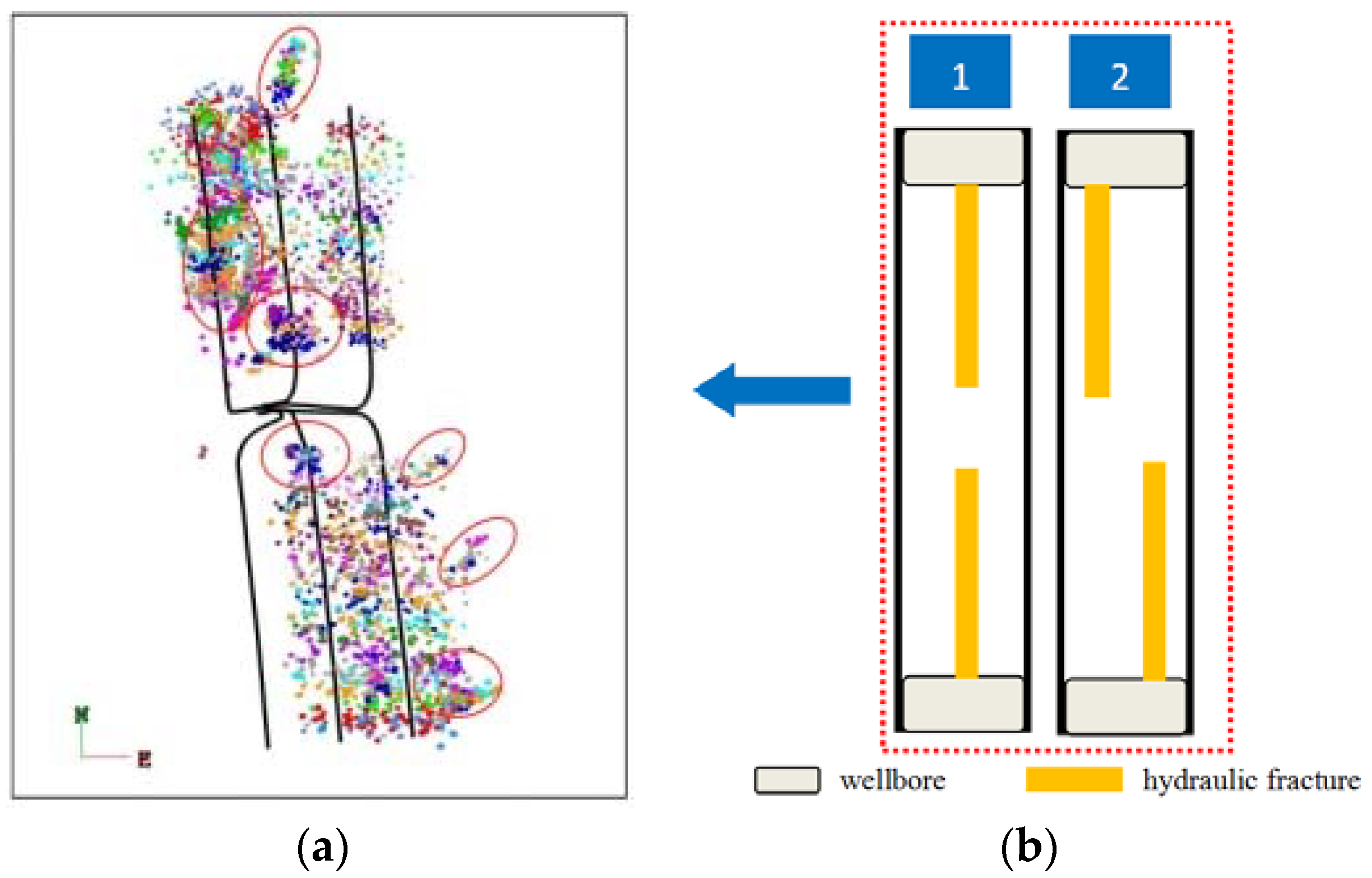
2.1. Conceptual Model

2.1.1. WIPS Scheme

Figure 1 illustrates the WIPS schemes in a tight oil reservoir. The whole oil field can consist of several independent WIPS scheme. Although every WIPS scheme also can interfere with each other when the wells produce enough long time, in this paper, we mainly focus on WIPS within one WIPS scheme at the early-intermediate production period. Each WIPS scheme contains several SMFHWs which produce using same platform. Figure 1a,b illustrate the micro-seismic surveillance within one WIPS scheme and the corresponding idealized scenarios of hydraulic fractures.

2.1.2. Tight Oil Formation Model

Because the reservoir thickness is much smaller than its radius, the conceptual model of tight formation can be interpreted as a two-dimensional flat. Tight reservoirs are assumed to be isotropic reservoirs, including natural fractures (NFs) systems and matrix systems, and bounded by upper and lower impermeable formations.

In order to describe our method conveniently, we chose two SMFHWs for our research purpose. However, our approach can be easily extended to more than three SMFHWs WIPS scenarios. Two SMFHWs produced at constant oil rate q₁ and q₂. Fluid flows into HFs from tight oil reservoir and is assumed to q_f. In addition, there are some other assumptions as follows:

• hydraulic fractures in horizontal wells are distributed symmetrically and penetrate the reservoir completely;
• The thickness of reservoir is h, the initial pressure is Pi and the initial temperature is T;
• Fluid flow in NFs system and matrix satisfies Darcy’s law. Natural fractures (NFs) system consider the effect of stress sensitivity;
• Considering the compressibility of fluid, assuming the compression coefficient is a constant value;
• Neglecting the influence of gravity and capillary force;
• Wellbore storage is considered.

2.2. Mathematical Model

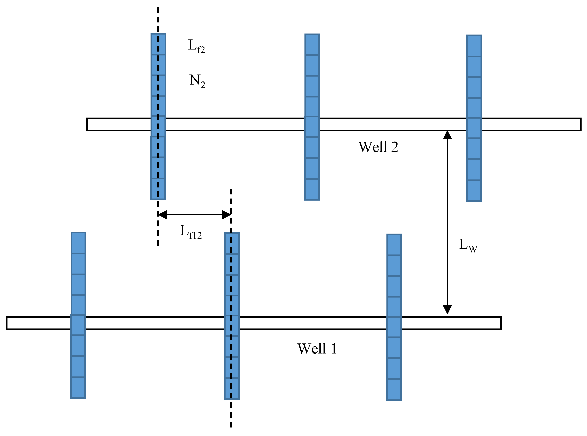
2.2.1. Parameter Description of HFs

As shown in Figure 2, for well1, the fracture permeability is k_f1, the fracture width is w_f1, the fracture half-length is L_f1. For well2, the fracture permeability is k_f2, the fracture width is w_f2, the fracture half-length is L_f2. The distance between two well is L_w. the distance of two hydraulic fractures is L_f12. To establish a mathematical model, we first subdivide the HFs systems of WIPS scheme. We assume that each hydraulic fracture of well1 is divided into N₁ sub-fracture segments, each hydraulic fracture of well2 is divided into N₂ sub-fracture segments. The hydraulic fracture number of well1 is M₁. The hydraulic fracture number of well2 is M₂. The length of each fracture segment for well1 and well2 can be presented as ΔL_f1, ΔL_f2, respectively. We can summarize fracture properties as follows:

• Well 1: N₁, M₁, L_f1, ΔL_f1
• Well 2: N₂, M₂, L_f2, ΔL_f2

2.2.2. Seepage Model in Tight Reservoir System

We characterized tight reservoir as dual-porosity continuum and fracture system. Fluid flow in the fracture is considered compressible and can be described as a one-dimensional coordinate system (Figure 3). To obtain the solution in dual-porosity continuum, line-source function was a feasible approach [22,23]. After considering mass conservation principle, Darcy theory and motion equation, one can obtain the governing functions in dual-porosity continuum in Laplace domain as follows,

$$\frac{d^2\overline{\eta }}{d{r}_D^2}+\frac{1}{r_D}\frac{d\overline{\eta }}{d{r}_D}+\lambda \left(\overline{P_{mD}}-\overline{\eta }\right)=\omega S\overline{\eta }$$

(1)

$$-\lambda \left(\overline{P_{mD}}-\overline{\eta }\right)=\left(1-\omega \right)s\overline{P_{mD}}$$

(2)

After substituting the fluid transferring from matrix into natural fracture system, the flow equations in the fractured system of is

$$\frac{d^2\overline{\eta }}{d{r}_D^2}+\frac{1}{r_D}\frac{d\overline{\eta }}{d{r}_D}=f\left(s\right)\overline{\eta }$$

(3)

where, $f\left(s\right)=\frac{\left(1-\omega \right)s\lambda }{\left(1-\omega \right)s+\lambda }+\omega s$.

The inner-boundary condition for a linear source can be as follows:

$$r_D\frac{d\overline{\eta }}{d{r}_D}{|}_{r_D\to 0}=-\overline{q_D}$$

(4)

The outer-boundary condition for an infinite reservoir is

$$\overline{\eta }{|}_{r_D\to \infty }=0$$

(5)

Based on the solution for a fully penetrating fracture is obtained [3,4], the general solution of Equation (3) can be given by

$$\overline{\eta }\left(S,r_D\right)=A{I}_0\left(\sqrt{f\left(s\right)}{r}_D\right)+B{K}_0\left(\sqrt{f\left(s\right)}{r}_D\right)$$

(6)

According to the boundary conditions, we have A = 0 in Equation (4). Then, Equation (6) can be simplified

$$\overline{\eta }\left(S,r_D\right)=\overline{q_D}{K}_0\left(\sqrt{f\left(s\right)}{r}_D\right)$$

(7)

Using the principle of integration, pressure distribution at any random location (x_D, y_D) can be obtained

$$\overline{\eta }\left(S,x_D,y_D,x_{wD},y_{wD}\right)=\frac{\overline{q_D}}{\Delta L_{iD}}{{\displaystyle \int }}_{x_{wD}-\Delta L_{iD}/2}^{x_{wD}+\Delta L_{iD}/2}{K}_0\left[\sqrt{f\left(s\right)}\sqrt{\left(x_D-u\right)+{\left(y_D-y_{wD}\right)}^2}\right]du$$

(8)

2.2.3. Seepage Model in Hydraulic Fracture System

Semi-analytical method has been proposed to study the fluid flow within fracture system. Jia et al. [22], Zeng et al. [23] analyzed the unsteady state flow with considering fluid compressibility and rate accumulation, while Chen et al. [24] and Zhou et al. [25] analyzed the pseudo-steady state flow without considering fluid compressibility and rate accumulation. In our paper, we will establish a general model by considering the fluid compressibility and rate accumulation. When the fluid compressibility tends to be zero, the model can be equivalent to be a steady model.

Fluid flow in Hydraulic Fracture System can be presented as follows:

$$\frac{{\partial }^2{P}_{fD}}{\partial l_D^2}-\frac{2\mathsf{\pi }{q}_{fD}\left(l_D\right)}{C_{fD}\left(l_D\right)}=\frac{1}{C_{\eta D}}\frac{\partial P_{fD}}{\partial t_D}$$

(9)

And initial condition,

$$P_{fD}{|}_{t_D=0}=0$$

(10)

Inner boundary contact with wellbore, thus

$$\frac{\partial P_{fD}}{\partial l_D}{|}_{l_D=0}=\frac{q_{cD}\left(0\right)}{C_{fD}}$$

(11)

And there is no flow at the end of the fracture, so the outer boundary condition is

$$\frac{\partial P_{fD}}{\partial l_D}{|}_{l_D=L_{fD}}=0$$

(12)

2.3. Transient Pressure Analysis for WIPS Scheme

2.3.1. Tight Oil Reservoir System

Traditionally, we used the superposition principle to calculate the pressure response of SMFHWs. Similarly, superposition principle was applied in our new model with WIPS scheme. Based on Equation (8), using the principle of integration, pressure distribution at the center of HFs system can be obtained:

$$\begin{gathered} \overline{P_D}\left(x_{Do},y_{Do}\right)={\displaystyle \sum }_{a=1}^{M_1}{\displaystyle \sum }_{b=j}^{N_1}\frac{\overline{q_{fi,jD}}}{\Delta L_{f1D}}\overline{P_{uD}}\left(x_{D0},y_{D0},x_{Da,b},y_{Da,b}\right)+{\displaystyle \sum }_{i=1}^{M_2}{\displaystyle \sum }_{i=j}^{N_2}\frac{\overline{q_{fi,jD}}}{\Delta L_{f2D}}\overline{P_{uD}}\left(x_{D0},y_{D0},x_{Di,j},y_{Di,j}\right) \\ o=1,\dots ,\left(M_1\times N_1+M_2\times N_2\right) \end{gathered}$$

(13)

where

$$\overline{P_{uD}}\left(x_{D0},y_{D0},x_{Da,b},y_{Da,b}\right)={{\displaystyle \int }}_{x_{Da,b}-\Delta L_{f1D}/2}^{x_{Da,b}+\Delta L_{f1D}/2}{K}_0\left[\sqrt{f\left(s\right)}\sqrt{\left(x_{Do}-u\right)+{\left(y_{Do}-y_{Da,b}\right)}^2}\right]du$$

(14)

$$\overline{P_{uD}}\left(x_{D0},y_{D0},x_{Di,i},y_{Di,i}\right)={{\displaystyle \int }}_{x_{Di,i}-\Delta L_{f2D}/2}^{x_{Di,i}+\Delta L_{f2D}/2}{K}_0\left[\sqrt{f\left(s\right)}\sqrt{\left(x_{Do}-u\right)+{\left(y_{Do}-y_{Di,j}\right)}^2}\right]du$$

(15)

$\overline{P_{uD}}\left(x_{D0},y_{D0},x_{Da,b},y_{Da,b}\right)$ is the pressure response due to the fluid flow in hydraulic fracture of horizontal well1; $\overline{P_{uD}}\left(x_{D0},y_{D0},x_{Di,i},y_{Di,i}\right)$ is the pressure response due to the fluid flow in hydraulic fracture of horizontal well2.

2.3.2. HFs System

As shown in Figure 4, we can choose i-th fracture segment to analyze the flow equation in HFs System. Fluid in HFs System flow from ${\epsilon }_{i1}$ to ${\epsilon }_{i2}$. Hence, on the basis of Equation (9), the dimensionless governing function for this segment can be presented:

$$\frac{d^2\overline{P_{FD}}}{d{\epsilon }_D^2}-\frac{2\mathsf{\pi }}{C_{FD}}·\overline{q_{ciD}}=\frac{u}{C_{\eta D}}\overline{P_{FD}}$$

(16)

and boundary conditions at ${\epsilon }_{i1}$ and ${\epsilon }_{i2}$ given by

$$\frac{d\overline{P_{FD}}}{d{\epsilon }_D}{|}_{{\epsilon }_D={\epsilon }_{i1D}}=\frac{2\mathsf{\pi }}{C_{FD}}\overline{q_{cD}\left({\epsilon }_{i1D}\right)}$$

(17)

$$\frac{d\overline{P_{FD}}}{d{\epsilon }_D}{|}_{{\epsilon }_D={\epsilon }_{i2D}}=\frac{2\mathsf{\pi }}{C_{FD}}\overline{q_{cD}\left({\epsilon }_{i2D}\right)}$$

(18)

Combining with Equations (16) to (18), the pressure distribution of the i-th fracture segment can be obtained. Zeng’s method was applied to solve the fluid flow in the fracture segments [24]. The fluid flow equation of i-th fracture segment can be obtained by Laplace transformation.

$$\overline{P_{iD}}\left({\epsilon }_D,u\right)=b_i\left({\epsilon }_D\right)\overline{q_{ci2D}}+c_i\left({\epsilon }_D\right)\overline{q_{ci1D}}+d_i\overline{q_{FiD}}$$

(19)

Therefore, pressure of i-th fracture segment can be obtained

$$\overline{P_{icD}}\left(\frac{{\epsilon }_{i1D}+{\epsilon }_{i2D}}{2},u\right)=b_i\left(\frac{{\epsilon }_{i1D}+{\epsilon }_{i2D}}{2}\right)\overline{q_{ci2D}}+c_i\left(\frac{{\epsilon }_{i1D}+{\epsilon }_{i2D}}{2}\right)\overline{q_{ci1D}}+d_i\overline{q_{FiD}}$$

(20)

where

$$b_i\left({\epsilon }_D\right)=\frac{2\mathsf{\pi }}{C_{FD}\sqrt{\raisebox{1ex}{$u$}\!\left/ \!\raisebox{-1ex}{$C_{\eta D}$}\right.}}\left\{\frac{2cosh\left[\left({\epsilon }_D-{\epsilon }_{i1D}\right)\sqrt{\raisebox{1ex}{$u$}\!\left/ \!\raisebox{-1ex}{$C_{\eta D}$}\right.}\right]}{e^{2\left({\epsilon }_{i2D}-{\epsilon }_{i1D}\right)\sqrt{\raisebox{1ex}{$u$}\!\left/ \!\raisebox{-1ex}{$C_{\eta D}$}\right.}}-1}\right\}+e^{-\left({\epsilon }_D-{\epsilon }_{i1D}\right)\sqrt{\raisebox{1ex}{$u$}\!\left/ \!\raisebox{-1ex}{$C_{\eta D}$}\right.}}$$

(21)

$$c_i\left({\epsilon }_D\right)=\frac{-2\mathsf{\pi }}{C_{FD}\sqrt{\raisebox{1ex}{$u$}\!\left/ \!\raisebox{-1ex}{$C_{\eta D}$}\right.}}\left\{\frac{2cosh\left[\left({\epsilon }_{i2D}-{\epsilon }_D\right)\sqrt{\raisebox{1ex}{$u$}\!\left/ \!\raisebox{-1ex}{$C_{\eta D}$}\right.}\right]}{e^{2\left({\epsilon }_{i2D}-{\epsilon }_{i1D}\right)\sqrt{\raisebox{1ex}{$u$}\!\left/ \!\raisebox{-1ex}{$C_{\eta D}$}\right.}}-1}\right\}+e^{-\left({\epsilon }_{i2D}-{\epsilon }_D\right)\sqrt{\raisebox{1ex}{$u$}\!\left/ \!\raisebox{-1ex}{$C_{\eta D}$}\right.}}$$

(22)

$$d_i\left({\epsilon }_D\right)=\frac{-2\mathsf{\pi }{C}_{\eta D}}{C_{FD}u}$$

(23)

2.3.3. Solution Methodology

Observation from the proposed equations, there are three unknowns for each fracture segment: $\overline{P_{fDi1}}$, $\overline{q_{cDi1}}$, $\overline{q_{fDi1}}$. Then, the total number of unknowns are equal to [3(M₁ × N₁ + M₂ × N₂) + 2]. We can obtain a closed [3(M₁ × N₁ + M₂ × N₂) + 2]-order matrix from the following conditions:

For each fracture segment, the pressure obtained from reservoir fluid flow calculation and fluid flow calculation should be equal.

$$\overline{P_D}\left(x_{Di},y_{Di}\right)=\overline{P_{icD}}$$

(24)

Equation (24) applies to every fracture segment, so we can obtain more (M₁ × N₁ + M₂ × N₂)-equations.

Besides, the fluid rate and pressure at adjacent joints between two fracture segments should be same, namely,

$$q_{ci2D}=q_{c\left(i+1\right)1D}$$

(25)

$$b_i\left({\epsilon }_{i2D}\right)\overline{q_{ci2D}}+c_i\left({\epsilon }_{i2D}\right)\overline{q_{ci1D}}+d_i\overline{q_{FiD}}=\overline{P_{\left(i+1\right)D}}\left({\epsilon }_{\left(i+1\right)1D},u\right)$$

(26)

Another two equations are required to form a closed matrix. Well1 and well2 is produced at constant rate q₁ and q₂, respectively. Here, we define a new variable α, represents the ratio between q₁ and (q₁ + q₂), namely, $\epsilon =q_1/\left(q_1+q_2\right)$. Therefore,

$${\displaystyle \sum }_{i=1}^{M_1}\overline{q_{cDi\left(0\right)}}=\frac{\epsilon }{u}$$

(27)

$${\displaystyle \sum }_{i=1}^{M_2}\overline{q_{cD2\left(0\right)}}=\frac{1-\epsilon }{u}$$

(28)

Finally, we can obtain a closed [3(M₁ × N₁ + M₂ × N₂) + 2]-order matrix. Gauss elimination and Stehfest numerical algorithm [26] can be used to obtain pressure distribution solutions for the new model with WIPs scheme. Because of the solution in Laplace domain, the wellbore storage and skin factor can be easily added into the solution according to Duhamel’s theorem. Therefore, the solution can be presented as follows:

$${\overline{\eta }}_{Dwfin1}=\frac{{\overline{\eta }}_{Dwf1}/\epsilon }{1+u^2{C}_{D1}{\overline{\eta }}_{Dwf1}/\epsilon }$$

(29)

$${\overline{\eta }}_{Dwfin2}=\frac{{\overline{\eta }}_{Dwf2}/\left(1-\epsilon \right)}{1+u^2{C}_{D2}{\overline{\eta }}_{Dwf2}/\left(1-\epsilon \right)}$$

(30)

where, C_D1, C_D1 are dimensionless wellbore storage coefficient for well1 and well2 which are defined as ${\mathrm{C}}_{D1}=\frac{C_1}{2\mathsf{\pi }{L}_{ref}^{2}h\varphi C_t}$, ${\mathrm{C}}_{D2}=\frac{C_2}{2\mathsf{\pi }{L}_{ref}^{2}h\varphi C_t}$.

The stress sensitivity of NFs also can be taken into consideration. The bottom hole pressure in real space can be easily obtained Using the Stehfest numerical invention algorithm [26].

$$P_{WfD1}=-\frac{1}{{\zeta }_D}\ln \left(1-{\zeta }_D{\eta }_{Dwfin1}\right)$$

(31)

$$P_{WfD2}=-\frac{1}{{\zeta }_D}\ln \left(1-{\zeta }_D{\eta }_{Dwfin2}\right)$$

(32)

To analyze well performance in WIPS, Dimensionless multiwell productivity index $J_{1D}$ and $J_{2D}$, can be given as,

$$J_{1D} =\frac{B\mu q_1/\left(P_1-P_2\right)}{2\mathsf{\pi }{K}_{ri}h}=\frac{1}{P_{wfD1}}, J_{2D}=\frac{B\mu q_2/\left(P_1-P_2\right)}{2\mathsf{\pi }{K}_{ri}h}=\frac{1}{P_{wf{D}_2}}$$

(33)

3. Results and Discussion

In this section, three cases are studied, (I) model verification, (II) identification of flow regimes, and (III) sensitivity analysis. Case I is used for model verification using numerical simulation; Case II is applied to identify flow regimes based on special pressure-transient characteristics; Case III is sensitivity analysis of key parameters on pressure-transient response of WIPS scheme. The relevant parameters are shown in

Table 1. The basic input parameters in numerical simulation.

Type	Parameters	Value
Reservoir	Initial reservoir pressure, Pi (MPa)	25
	Formation temperature, T (K)	330
	Formation thickness, h (m)	10
	Total compressibility of reservoir, Ct (MPa−1)	2.5 × 10−4
	Porosity of reservoir Φ (fraction)	0.06
	Reservoir area, (m × m)	1000 × 500
	Initial natural fracture permeability, kri (D)	0.001
Well1	Hydraulic fracture permeability, kf1 (D)	10
	Hydraulic-fracture width, wf1 (m)	0.005
	Hydraulic-fracture half-length, Lf1 (m)	30
	Hydraulic-fracture number, M1	4
	Total compressibility of hydraulic fracture, Ctf1 (MPa−1)	3.5 × 10−4
	Hydraulic-fracture porosity, Φf1 (fraction)	0.35
	Wellbore length, Lw1 (m)	1000
Well2	Hydraulic fracture permeability, kf2 (D)	10
	Hydraulic-fracture width, wf2 (m)	0.005
	Hydraulic-fracture half-length, Lf2 (m)	30
	Hydraulic-fracture number, M2	4
	Total compressibility of hydraulic fracture, Ctf2 (MPa−1)	3.5 × 10−4
	Hydraulic-fracture porosity, Φf2 (fraction)	0.35
	Wellbore length, Lw2 (m)	1000

.

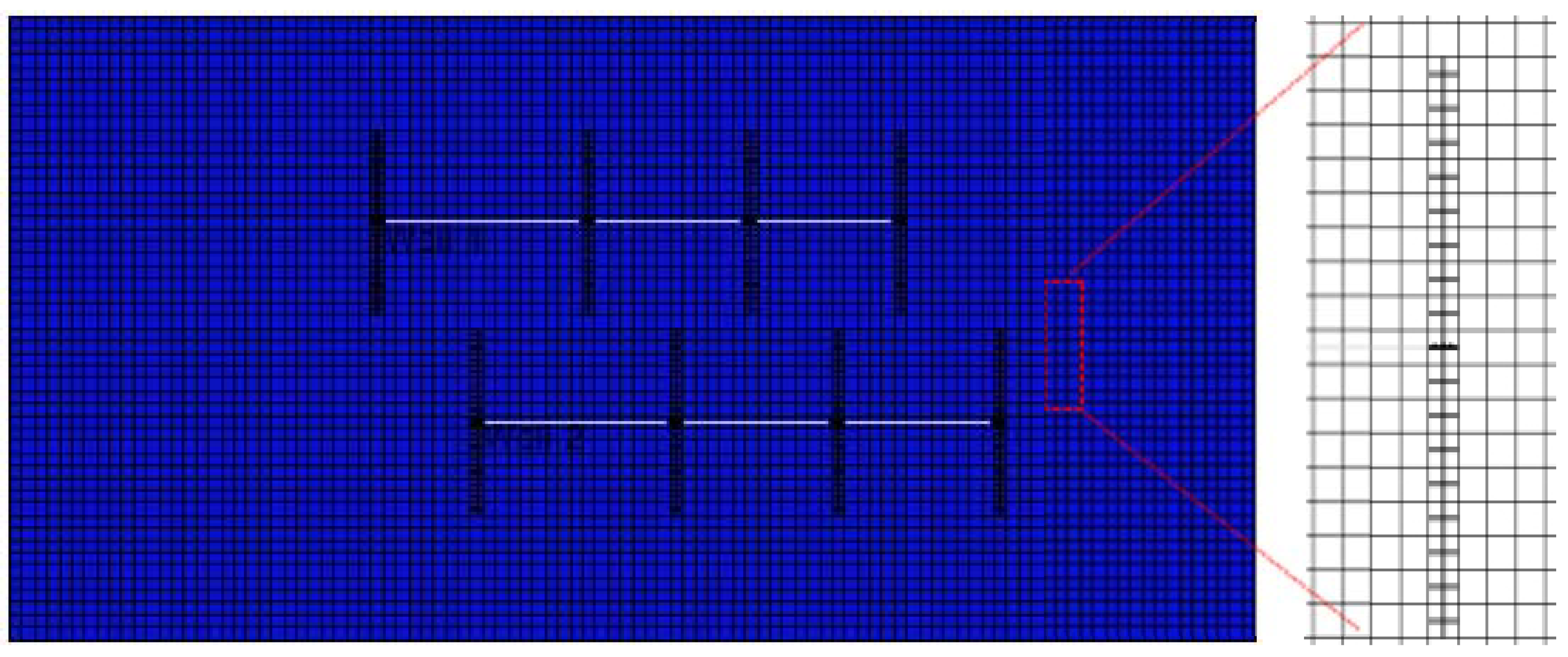
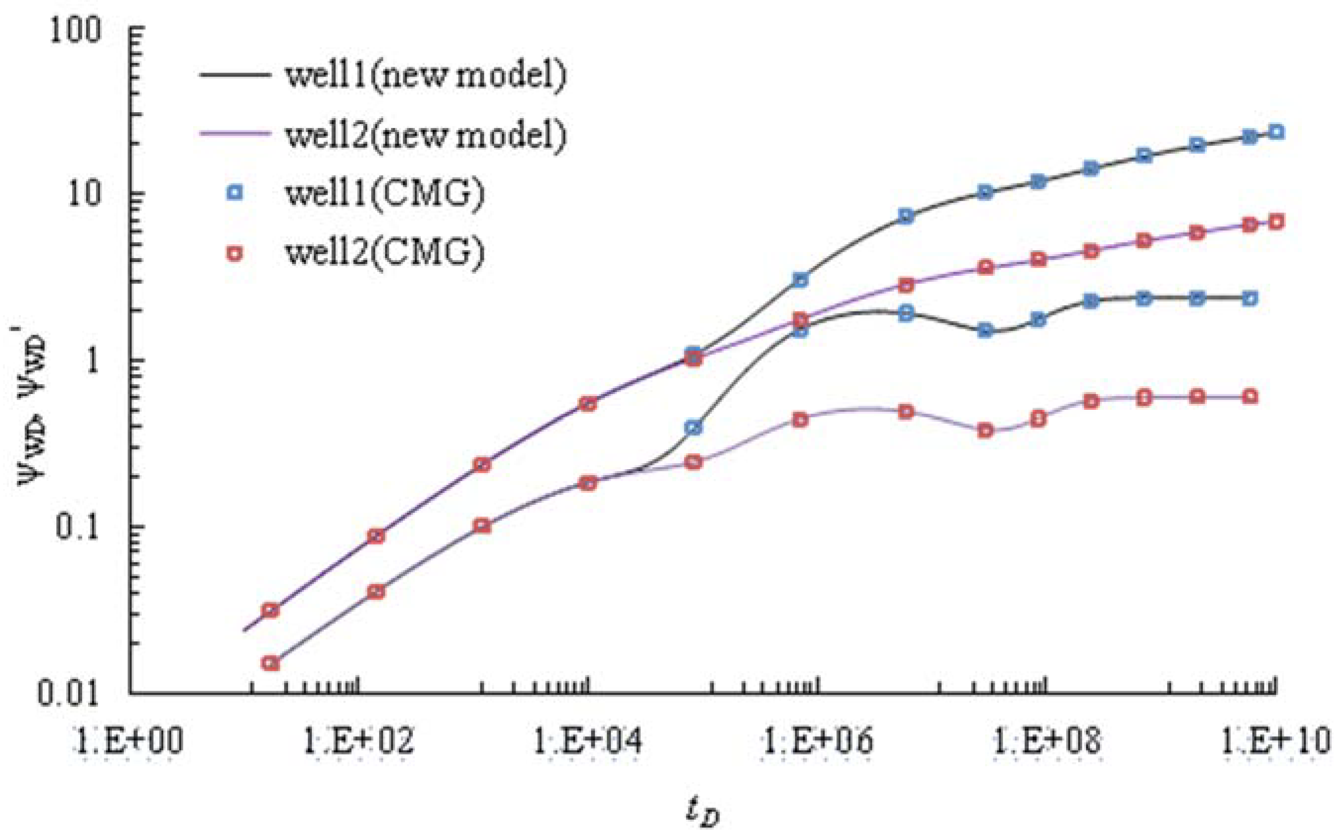
3.1. Model Validation

At present, there is no analytical or semi-analytic model for multi-well interference. Therefore, we choose commercial software to verify the accuracy of our model, CMG-2010 (Computer Management Group Ltd., Calgary, AB, Canada), and the top view of WIPS scheme is shown in Figure 5. The numerical simulation model consists of two horizontal wells. Each horizontal well contains four hydraulic fractures with a fracture spacing of 250 m. Double klinkenberg permeability- logarithmic spacing-local grid refinement (DK-LS-LGR) technology was used to characterize hydraulic fractures system. To avoid the same pressure type curve between the two horizontal wells, the oil ratio was assumed to 1:4. As shown in Figure 6, we can get a good fit between the numerical simulation and the theoretical model, which shows that the new model is reliable.

On the premise of ensuring the accuracy of the model, we tested the calculation speed of the model. Under the same hardware condition, the running time of the semi-analytical model and the numerical simulation model were 245.2 and 273.5 s, respectively.

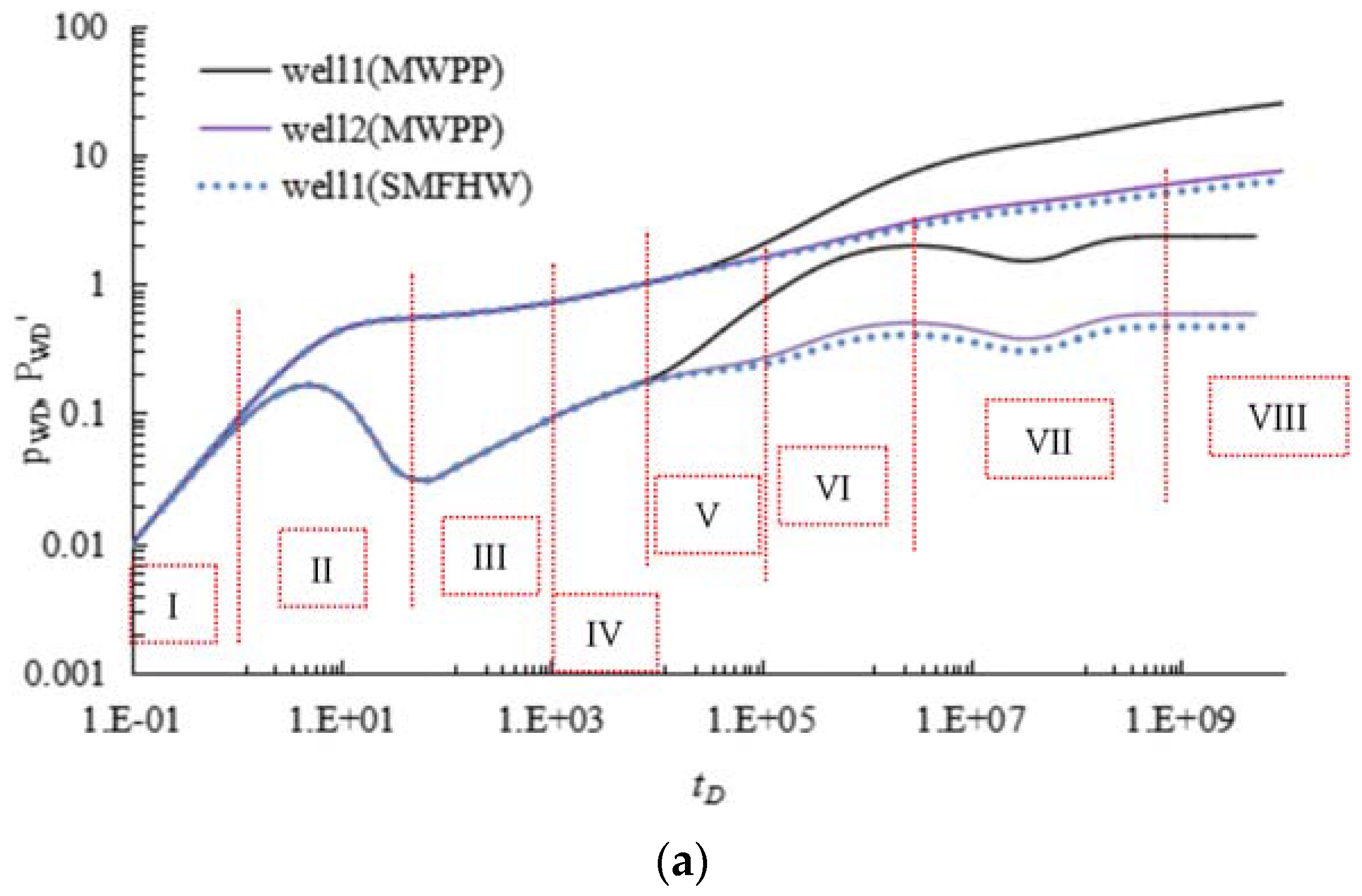
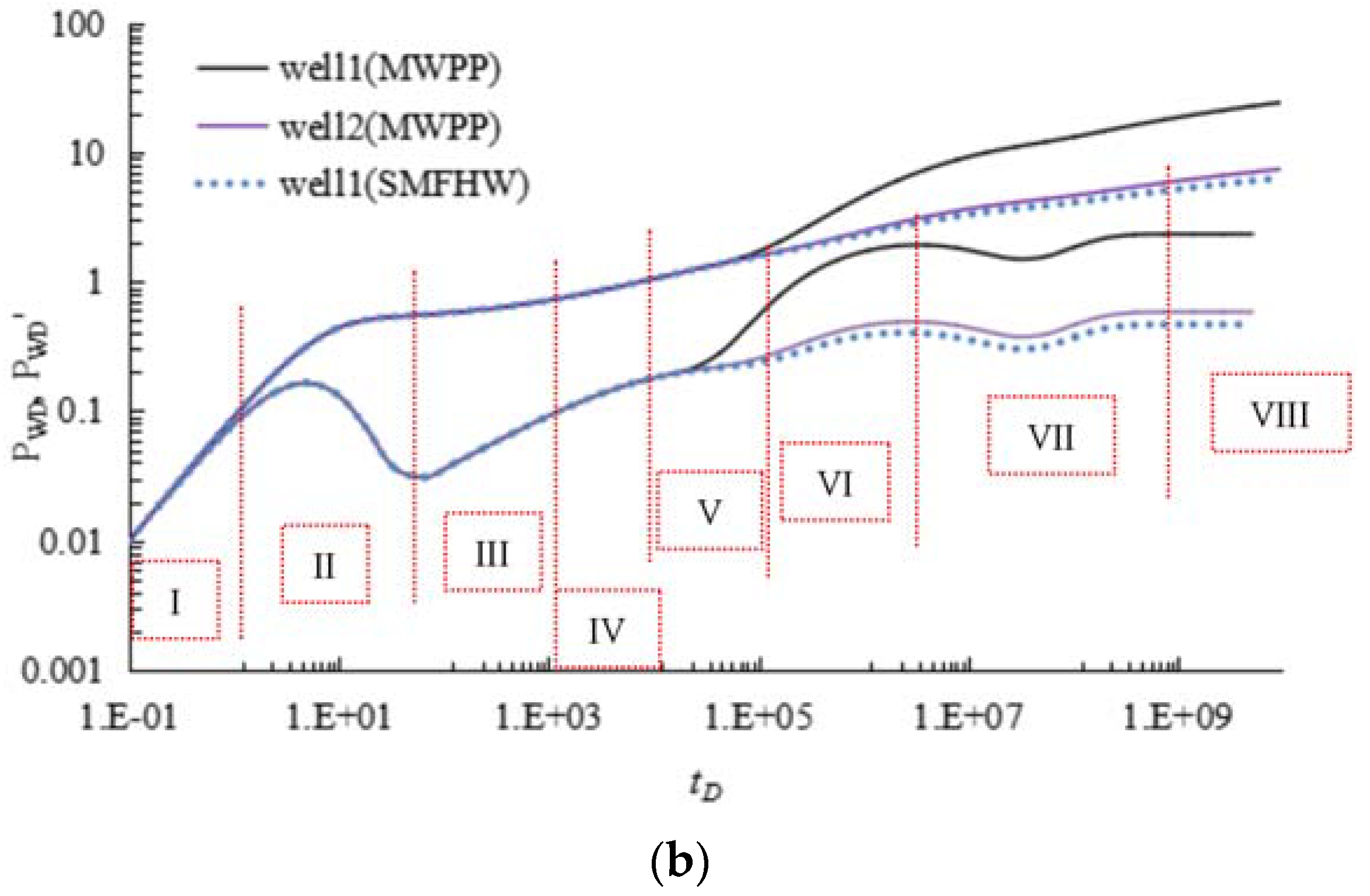
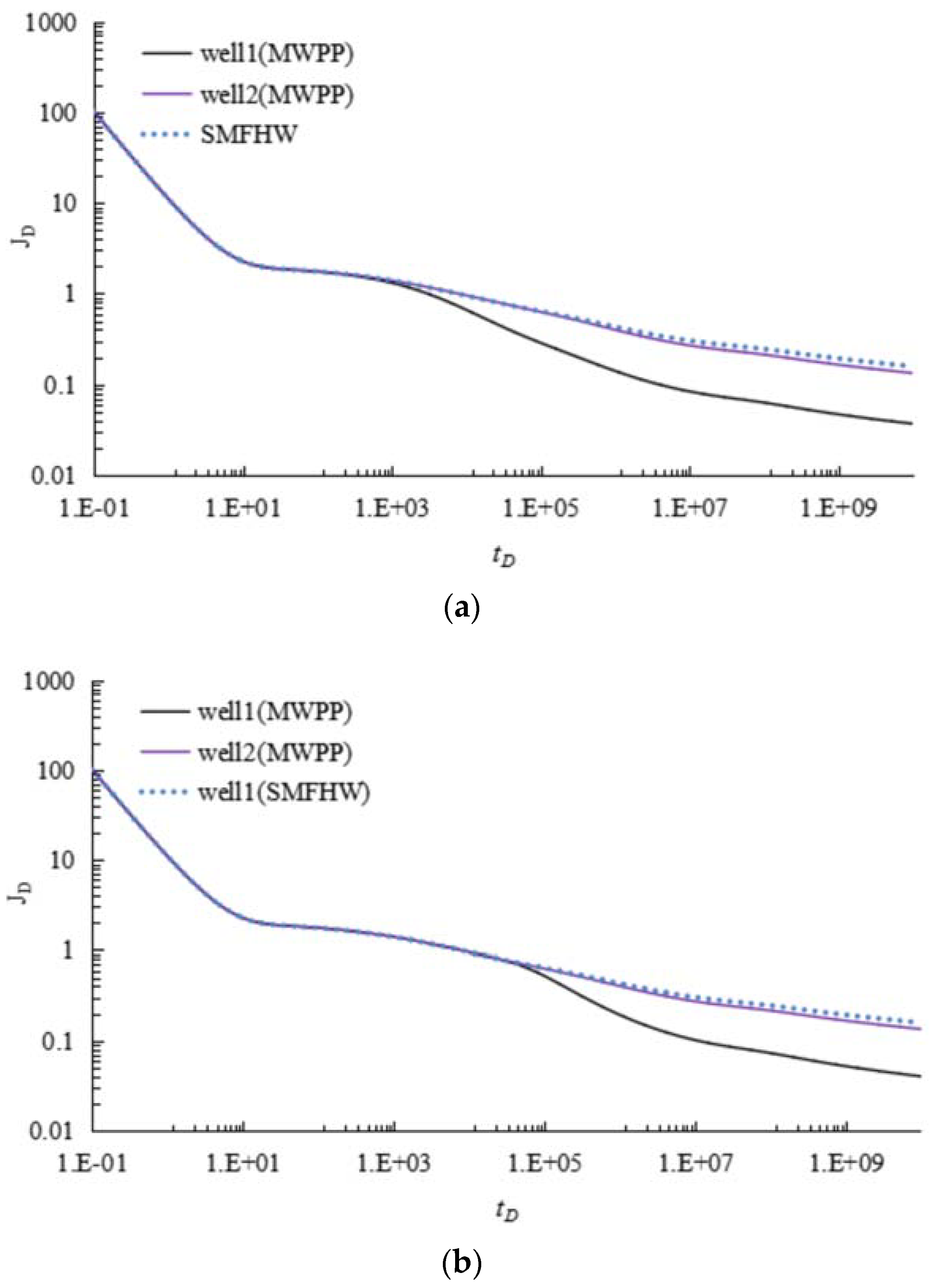
3.2. Identification of MWPI Using Flow Regime

In this section, we will mainly focus on identifying the MWPI phenomenon based on the special characteristic of pressure response curves. Common parameters were set for those two wells: M₁ = 3, M₂ = 3, ζ_D = 0.05, λ=0.002, γ = 0.15, ω = 0.0035, C_ηD = 10⁵. Setting consistent fracture properties (conductivity and half-length) L_f1D = L_fD2 = 200, C_f1D = C_f2D = 10. Another two parameters, L_wD and L_f12D, can be mathematically described as follows:

• Figure 1b (1): L_wD =L_f1D + L_fD2 + 100 = 500, and L_f12D = 0;
• Figure 1b (2): L_wD =L_f1D + L_fD2 + 100 = 500, and L_f12D = 500.

Dimensionless pressure (DP) and the dimensionless pressure derivative (DPD) of WIPS scheme are shown in Figure 7. To clearly describe the type curves, we will compare the characteristics of pressure curves between WIPS and SMFHWs. By Comparing between SMFHWs and WIPS scheme, we can add some additional information and better explanation into these distorted flow regimes, which can be described in detail as follows:

Regime I: The pure wellbore storage period regime. DP curve and DPD curve align, and the slope of curves are equal to 1. This stage is mainly controlled by wellbore storage effect and difficult to be impacted by the MWPI. Thus, the type curve of WIPS and SMFHWs overlap with each other.

Regime II: The transition flow regime. The early stage of this regime gradually derives from the straight line which has unit slope. This stage is mainly controlled by fluid properties and also difficult to be impacted by MWPI. Thus, the type curve of WIPS and SMFHWs also overlap with each other.

Regime III: The linear flow regime within HFs. This stage is mainly dominated by fracture conductivity. At this linear flow regime, and also difficult to be impacted by MWPI. Thus, the type curve of WIPS and SMFHWs also overlap with each other.

Regime IV: The bi-linear flow regime. This stage is mainly controlled by fracture length. At this bi-linear flow regime, we can start to detect the MWPI for type Figure 1b (1). The slope of the DPD curves is actually bigger than 0.25. The distortion degree of pressure curve for small oil rate is also more significant than that of big oil rate. However, it is still difficult to be impacted by the MWPI for type Figure 1b (2), Thus, the type curve of WIPS and SMFHWs still overlap with each other.

Regime V: The early pseudo-radial flow regime. This stage is mainly dominated by fracture spacing. At this pseudo-radial flow regime, we can start to detect the MWPI for type Figure 1b(2). The slope of the DPD curves is actually bigger than 0. The distortion degree of pressure curve for small oil rate is more significant that that of big oil rate.

Regime VI: The intermediate-time linear flow regime. This stage is mainly dominated by wellbore length. At this intermediate-time linear flow regime, we also can detect the MWPI for type Figure 1b (1) and Figure 1b (2). The slope of the DPD curves is actually bigger than 0.5. The distortion degree of pressure curve for small oil rate is more significant that that of big oil rate.

Regime VII: The pseudo-steady diffusion regime between the matrix and natural fractures. The main feature of type curves is marked by a “dip” shape in DPD curves.

Regime VIII: The late-time pseudo-radial flow regime. The shape of DPD curve is a horizontal line. The value of this horizontal well is equal to 0.5.

This section can clearly demonstrate the existence of multi-well pressure interference in WIPS by using the transient-pressure analysis. Furthermore, to analyze the well performance in WIPS with the influence of multi-well pressure interference, Figure 8 illustrates the dimensionless multi-well productivity index. Comparing to the SMFHWs, the well performance severely decreases. Figure 8 also shows that the different location of fractures leads to different occurrence periods of multi-well pressure interference.

3.3. Sensitivity Analysis

In this section, we conduct some sensitivity analysis on MPI for WIPS scheme. The key factors that influence MPI for WIPS scheme include hydraulic fracture half-length L_fD, hydraulic fracture conductivity C_fD, hydraulic fracture spacing L_f12D, well spacing L_wD, ratio of well rate ε, stress sensitivity ζ_D. Some dimensionless parameters can be: S = 0.2, C_D = 10, ζ_D = 0.05, λ = 0.002, γ = 0.15, ω = 0.0035, C_ηD = 105, L_f1D = 2000, L_f2D = 2000, L_wD = 3000, L_f12D = 1000. C_f1D = 50, C_f1D = 50. The results are discussed in detail as follows:

3.3.1. Ratio of Well Rate, ε

We set ε to be 0.1, 0.3, 0.5 respectively. Figure 9 shows effects of ration of well rate on pressure performance for WIPS scheme. We can judge the occurrence of MWPI by whether the MPI curves of two wells overlap together. The smaller the well rate, the more severely the curves are distorted. Moreover, the smaller the well rate, the smaller the dimensionless multi-well productivity index. Therefore, we can judge the well rate of two wells based on the relative position of the MPI curves. We also can summarize that the ratio of well rate ε approximately has no any influence on the time when the MWPI occurs.

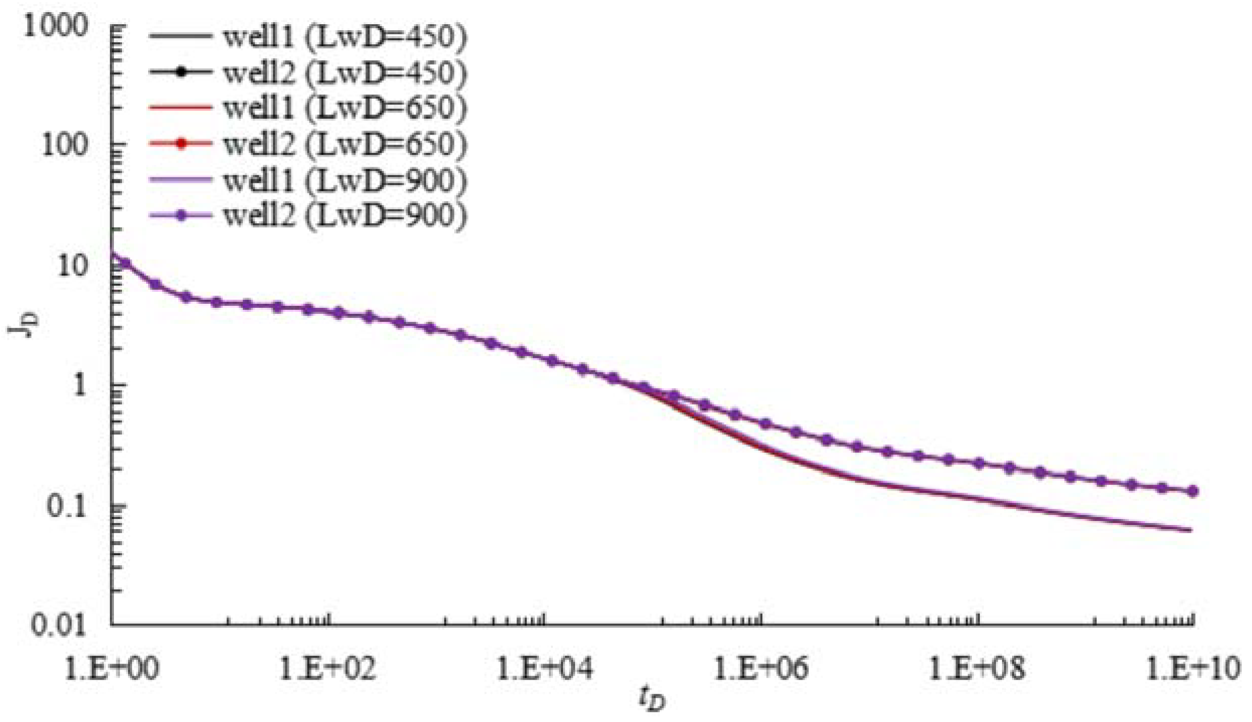
3.3.2. Well Spacing, L_wD

We set L_wD to be 450, 650, 900 respectively, and we also set ε to be 1:4. Figure 10 illustrates the impacts of well spacing L_wD on pressure performance for WIPS scheme. Similarly, we also can judge the occurrence of MWPI by whether MPI curves of two wells overlap together. On condition of different well spacing L_wD, MWPI basically starts form first radial-flow regimes. As the well spacing L_wD increases, the occurrence of MWPI becomes later, and thus MPI inversely increases. Besides, MPI curves will be split, the pressure curves will overlap again subsequently. We also can clearly observe another phenomenon that well spacing almost does not distort the shape of MPI curves, the MPI curves just move upward or downward (the slope of MPI curves keeps constant). When the oil rate is big enough, the impacts of well spacing on multi-well interference can hardly be identified (the dot line).

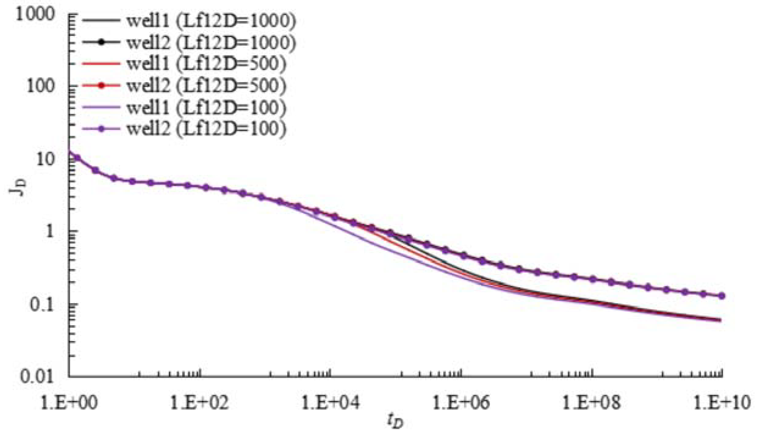
3.3.3. Hydraulic Fracture Spacing, L_f12D

We set L_f12D to be 100, 500, 1000 respectively, and we also set ε to be 1:4. Figure 11 illustrates the impacts of hydraulic fracture spacing L_f12D on pressure performance for WIPS scheme. Similar to the effects of well spacing on pressure curves, hydraulic fracture spacing mainly impacts the occurrence of MWPI and have no any influence on the distortion of flow regimes, the MPI curves just move upward or downward (the slope of MPI curves keeps constant). Different from the effects of well spacing, the impacts of fracture spacing is more significant than that of well spacing. When L_f12D = 100, MWPI basically starts from first linear-flow regime. When L_f12D = 1000, MWPI basically starts form first radial-flow regimes. As the fracture spacing L_f12D increases, the occurrence of MWPI becomes later and thus MPI inversely increases. Similarly, when the oil rate is big enough, the impacts of fracture spacing on well performance also cannot be observed from MPI curves.

3.3.4. Hydraulic Fracture Length, L_f1D, L_f2D

We set L_f1D = L_f2D = L_fD to be 1000, 1500, 2000 respectively and ε to be 1:4. Figure 12 illustrates the impacts of hydraulic fracture length L_fD on pressure performance for WIPS scheme. We can systematically analyze the impacts of L_fD on pressure performance from three aspects: (1) Before the occurrence of MWPI, for a certain fracture length, the pressure curves of two wells will overlap together. However, when fracture length is varying, the pressure curves will paralleled move upward or downward. As the fracture length increases, the pressure curves will paralleled move downward; (2) When the MWPI occurs, as the fracture length L_fD increases, the occurrence of MWPI becomes earlier. For example, when L_fD = 2000, MWPI basically starts form first linear-flow regime. When L_fD = 1000, MWPI basically starts form first bi-linear-flow regime; (3) When MWPI reaches certain degree, the pressure curves will overlap again subsequently. The bigger the oil rate, the more lately the pressure curves overlap. For example, for well1, the pressure curves will overlap at second linear-flow regime, for well2, the pressure curves will overlap at pseudo-steady diffusion regime. In conclusion, fracture length impacts the whole flow regimes for WIPS scheme.

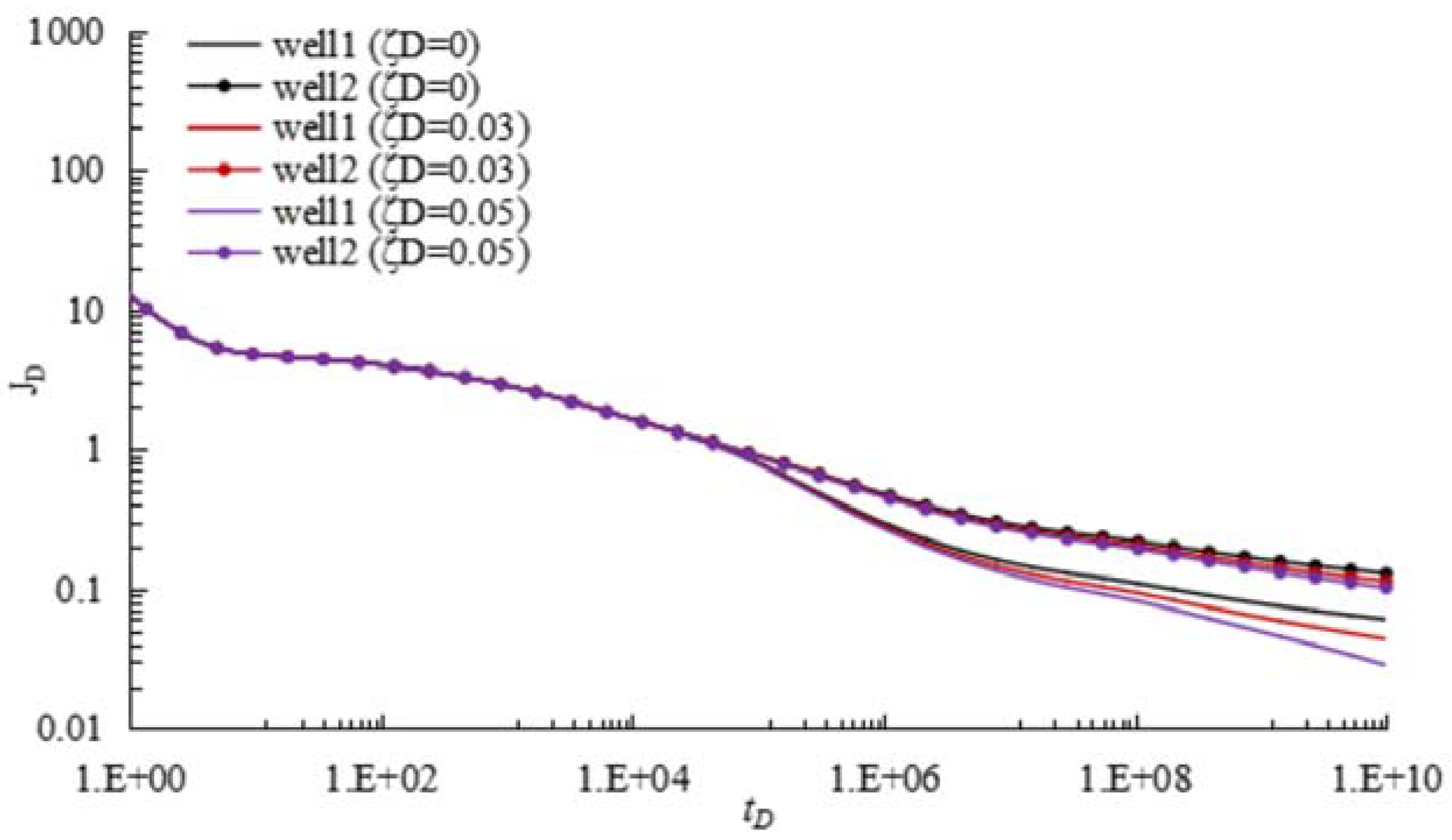
3.3.5. Stress Sensitivity Coefficient, ζ

We set ζ_D to be 0, 0.03, 0.05 respectively and ε to be 1:4. Figure 13 illustrates the impacts of stress sensitivity coefficient ζ_D on pressure performance for WIPS scheme. It is hardly to find that stress sensitivity coefficient has some influences on the occurrence of MWPI. However, stress sensitivity coefficient can distort flow regimes at an inverse direction. For example, when ζ = 0.03, radial-flow regimes and pseudo-steady diffusion regimes are distorted. When ζ = 0.05, radial-flow regimes, pseudo-steady diffusion regimes and second linear-flow regime are distorted. As the ζ increases, the distortion of pressure curves becomes severe, and more flow regimes will be distorted.

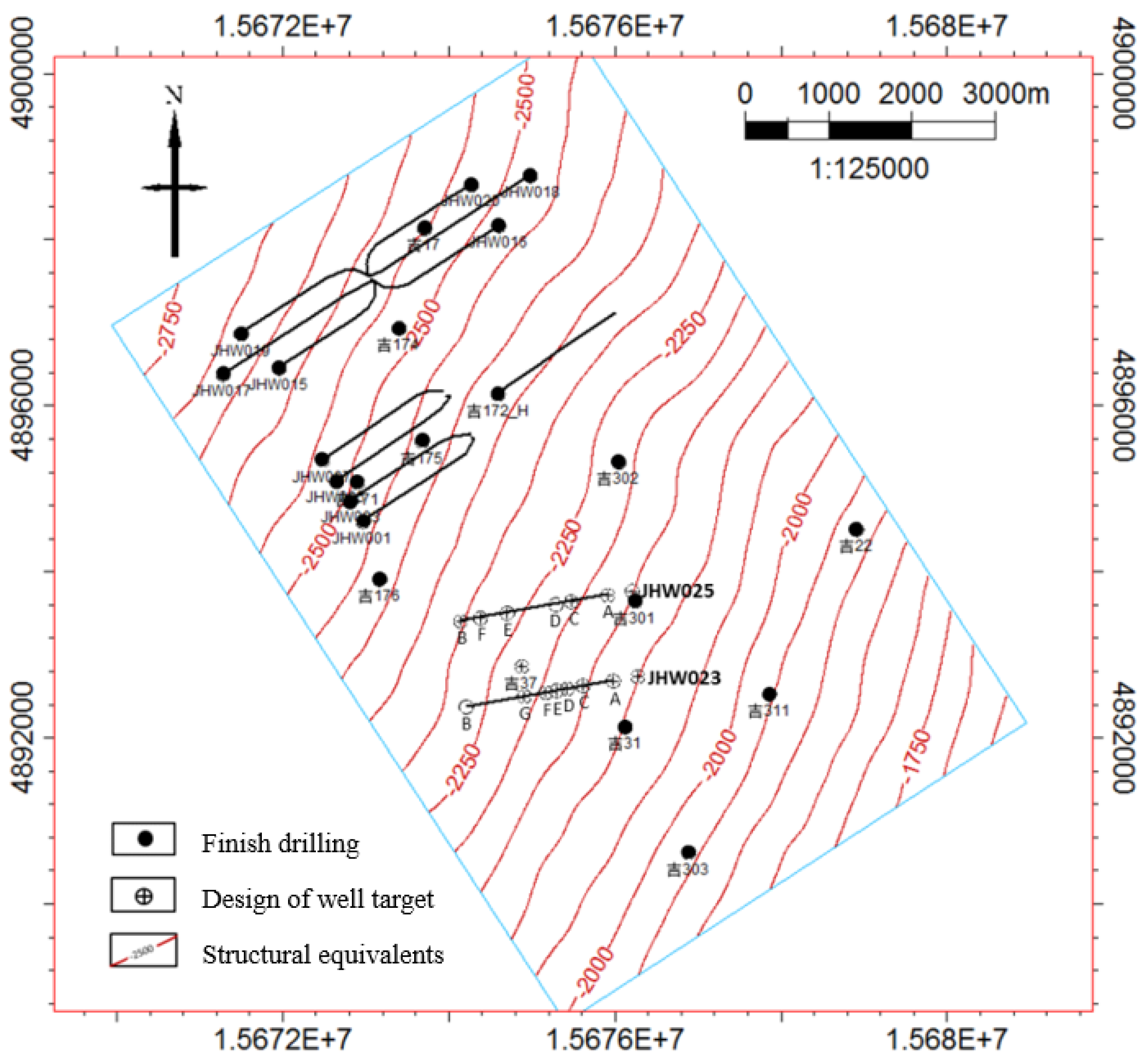
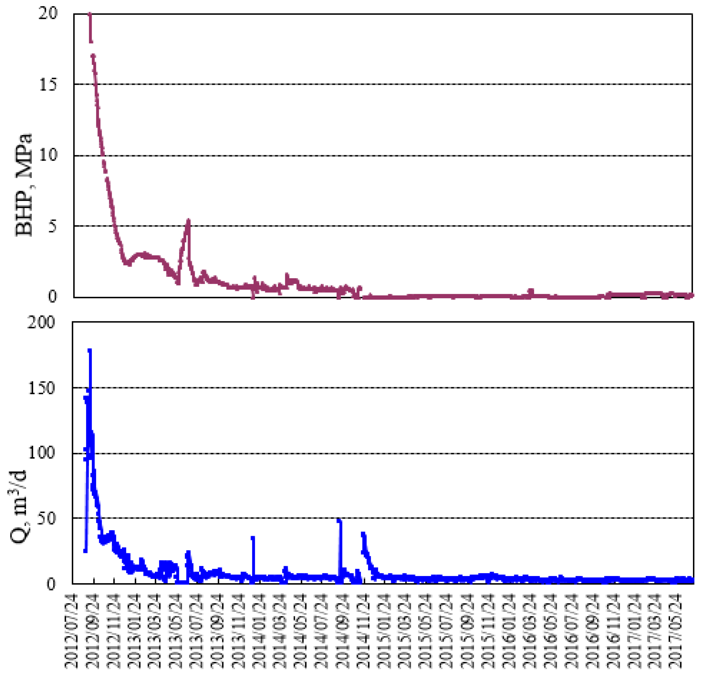
3.4. Case Application

In this section, we try to apply our methodology to a realistic case, Xinjiang Changji Oilfield is located in the east of the Zhungeer Basin, with an area of 1278 km² and 150 km away from Urumqi, administrative district belongs to the Jimsar County of Xinjiang Uygur Autonomous Region. According to drilling data, the formation thickness of the area is 28–75 m, an average of 53.5 m, The average porosity of the reservoir is 10.99% and the permeability is 0.012 mD, which belong to the typical tight oil reservoir. To improve the oil recovery, well-industry-production-scheme (WIPS) is used, the illustration of the WIPS can be found in Figure 14. Because of some policy limitation, more detailed information cannot be specified. Our target wells are located at the north-west corner. This WIPS has 6 horizontal wells. Some fracturing parameters can be found in

Table 2. Some fracturing parameters for the well-industry-production-scheme.

Well Names	JHW015	JHW016	JHW017	JHW018	JHW019	JHW020
Well length, m	1310	1312	1801	1732	1228	1304
Fracture stages	18	18	23	23	15	17
Half length, m	140	175	125	175	145	155
Porosity, %	10.99
Permeability, mD	0.012
Oil saturation, %	65

. Figure 15 shows the production scheme of the well JHW015, the production profile of other wells do not show here.

Given the specific parameters, including fracture length, number of fractures, well length, formation permeability, we estimate the well distance approximately using our proposed semi-analytical method. Here, we take the well JHW015 as an example to explain how to use our method. To begin with, the productivity index can be calculated using the historical production data, as Figure 15. Second, given some known parameters, several dimensionless productivity index curves can be plotted based on different well distance. Finally, we can match those curves to approximately estimate the possible well distance in this well-industry-production-scheme (WIPS). As one can see in Figure 16, at the early production stage, this is the fracturing fluid drawback from the formation with two-phase flow, as result, our model cannot match with this data, thus, we should avoid use the production data at the early production period. Based on the matching results of type curves, the well distance is slightly bigger than 500 m.

4. Conclusions

To gain better understanding of well performance of WIPS scheme, in this paper, a semi-analytical multi-well productivity index (MPI) model in Laplace domain is developed through considering the influences of MWPI. Through model validation and sensitivity analysis, some meaningful conclusions are summarized as follows:

• Avoiding complicated grid refinement, our proposed semi-analytical model provides promising calculation speed over numerical simulation, especially for complex fracture geometry.
• Compared to single multi-fractured horizontal wells (SMFHWs), our proposed multi-well pressure interference model has the abilities to identify the flow regimes with MWPI. Our results show that part of flow regimes are distorted by MWPI to some degree. The slope of type curves which characterize the linear or bi-linear flow regime is no longer equal to 0.5 or 0.25. The horizontal line which characterize radial flow regime is no longer equal to 0.5.
• Well rate mainly determines the distortion degree of MPI curves. Well rate will distort pressure and MPI curves when MWPI occurs. As the well rate decreases, the distortion of MPI curves will become severe.
• Fracture length, well spacing, fracture spacing mainly determine when the MWPI occurs. As the well spacing increases, fracture length decreases, fracture spacing decreases, the occurrence of MWPI becomes later. For well spacing, fracture spacing, when MWPI occurs, pressure curves splits, and then overlaps again. For fracture length, pressure curves will always split until MWPI reaches certain degree.
• Stress sensitivity coefficient mainly affects the MPI at the formation pseudo-radial flow stage, almost has no influence on the occurrence of MWPI. The bigger the stress sensitivity coefficient, the smaller the multi-well productivity index.
• Our application also shows promising aspects of our semi-analytical model to estimate the well distance between multi-wells for MWPP scheme, which is often uncertain in the hydraulic fracturing operation.

References

1. Tight Oil Expected to Make up Most of U.S. Oil Production Increase Through 2040. Available online: https://www.eia.gov/todayinenergy/detail.php?id=29932# (accessed on 22 February 2017).
2. Hu, J.; Zhang, C.; Rui, Z.; Yu, Y.; Chen, Z. Fractured horizontal well productivity prediction in tight oil reservoirs. J. Pet. Sci. Eng. 2017, 151, 159–168. [Google Scholar] [CrossRef]
3. Ozkan, E.; Raghavan, R. New solutions for well-test analysis problems. Part 1. Analytical considerations. SPE Form. Eval. 1991, 6, 359–368. [Google Scholar] [CrossRef]
4. Ozkan, E.; Raghavan, R. New Solutions for Well-Test-Analysis Problems: Part 2. Computational Considerations and Applications. SPE Form. Eval. 1991, 6, 369–378. [Google Scholar] [CrossRef]
5. Guo, G.; Evans, R.D. Pressure-Transient Behavior and Inflow Performance of Horizontal Wells Intersecting Discrete Fractures. In Proceedings of the SPE Annual Technical Conference and Exhibition, Houston, TX, USA, 3–6 October 1993. SPE 26446. [Google Scholar]
6. Wan, J.; Aziz, K. Semi-Analytical Well Model of Horizontal Wells with Multiple Hydraulic Fractures. SPE J. 2002, 7, 437–445. [Google Scholar] [CrossRef]
7. Al-Kobaisi, M.; Ozkan, E.; Kazemi, H. A Hybrid Numerical-Analytical Model of Finite-Conductivity Vertical Fractures Intercepted by a Horizontal Well. In Proceedings of the SPE International Petroleum Conference in Mexico, Puebla, Mexico, 7–9 November 2004. SPE 92040. [Google Scholar]
8. Mayerhofer, M.; Lolon, E.; Youngblood, J.; Heinze, J. Integration of Microseismic Fracture Mapping Results with Numerical Fracture Network Production Modeling in the Barnett Shale. In Proceedings of the SPE Annual Technical Conference and Exhibition, San Antonio, TX, USA, 24–27 September 2006. SPE 102103. [Google Scholar]
9. Ozkan, E.; Brown, M.; Raghavan, R.; Kazemi, H. Comparison of Fractured Horizontal-Well Performance in Conventional and Unconventional Reservoirs. Dermatol. Surg. 2009, 27, 703–708. [Google Scholar]
10. Ozkan, E.; Brown, M.L.; Raghavan, R.; Kazemi, H. Comparison of Fractured-Horizontal-Well Performance in Tight Sand and Shale Reservoirs. SPE Reserv. Eval. Eng. 2011, 14, 248–259. [Google Scholar] [CrossRef]
11. Brown, M.L.; Ozkan, E.; Raghavan, R.S.; Kazemi, H. Practical Solutions for Pressure Transient Responses of Fractured Horizontal Wells in Unconventional Reservoirs. J. Pet. Technol. 2010, 62, 63–64. [Google Scholar]
12. Brown, M.L.; Ozkan, E.; Raghavan, R.S.; Kazemi, H. Practical Solutions for Pressure-Transient Responses of Fractured Horizontal Wells in Unconventional Shale Reservoirs. SPE Reserv. Eval. Eng. 2011, 14, 663–676. [Google Scholar] [CrossRef]
13. Stalgorova, E.; Mattar, L. Practical Analytical Model to Simulate Production of Horizontal Wells with Branch Fractures. In Proceedings of the SPE Canadian Unconventional Resources Conference, Calgary, AB, Canada, 30 October–1 November 2012. SPE 162515. [Google Scholar]
14. Stalgorova, E.; Mattar, L. Analytical Model for History Matching and Forecasting Production in Multifrac Composite Systems. In Proceedings of the SPE Canadian Unconventional Resources Conference, Calgary, AB, Canada, 30 October–1 November 2012. SPE 162516. [Google Scholar]
15. Wang, L.; Wang, X.; Li, J.; Wang, J. Simulation of Pressure Transient Behavior for Asymmetrically Finite-Conductivity Fractured Wells in Coal Reservoirs. Transp. Porous Media 2013, 97, 353–372. [Google Scholar] [CrossRef]
16. Deng, J.; Zhu, W.; Ma, Q. A new seepage model for shale oil reservoir and productivity analysis of fractured well. Fuel 2014, 124, 232–240. [Google Scholar] [CrossRef]
17. Wang, W.; Shahvali, M.; Su, Y. A semi-analytical fractal model for production from tight oil reservoirs with hydraulically fractured horizontal wells. Fuel 2015, 158, 612–618. [Google Scholar] [CrossRef]
18. Fan, D.; Yao, J.; Hai, S.; Hui, Z.; Wei, W. A composite model of hydraulic fractured horizontal well with stimulated reservoir volume in tight oil & oil reservoir. J. Nat. Oil Sci. Eng. 2015, 24, 115–123. [Google Scholar]
19. Xiao, C.; Tian, L.; Yang, Y.; Zhang, Y.; Gu, D.; Chen, S. Comprehensive application of semi-analytical PTA and RTA to quantitatively determine abandonment pressure for CO2 storage in depleted shale oil reservoirs. J. Pet. Sci. Eng. 2016, 146, 813–831. [Google Scholar] [CrossRef]
20. Sardinha, C.M.; Petr, C.; Lehmann, J.; Pyecroft, J.F. Determining Interwell Connectivity and Reservoir Complexity through Frac Pressure Hits and Production Interference Analysis. In Proceedings of the SPE/CSUR Unconventional Resources Conference—Canada, October, Calgary, AB, Canada, 30 September–2 October 2014. SPE 171628. [Google Scholar]
21. Awada, A.; Santo, M.; Lougheed, D.; Xu, D.; Virues, C. Is That Interference? A Work Flow for Identifying and Analyzing Communication through Hydraulic Fractures in a Multiwell Pad. SPE J. 2016, 21, 1–554. [Google Scholar] [CrossRef]
22. Jia, P.; Cheng, L.; Huang, S.; Cao, R.; Xu, Z. A Semi-Analytical Model for Production Simulation of Complex Fracture Network in Unconventional Reservoirs. In Proceedings of the SPE/IATMI Asia Pacific Oil & Oil Conference and Exhibition, Nusa Dua, Bali, Indonesia, 20–22 October 2015. SPE 176227. [Google Scholar]
23. Zeng, F.B.; Zhao, G.; Liu, H. A New Model for Reservoirs with a Discrete-Fracture System. J. Can. Pet. Technol. 2012, 51, 127–136. [Google Scholar] [CrossRef]
24. Chen, Z.; Liao, X.; Zhao, X.; Lv, S.; Zhu, L. A Semianalytical Approach for Obtaining Type Curves of Multiple-Fractured Horizontal Wells with Secondary-Fracture Networks. SPE J. 2016, 21, 538–549. [Google Scholar] [CrossRef]
25. Zhou, W.; Banerjee, R.; Poe, B.; Spath, J.; Thambynayagam, M. Semianalytical Production Simulation of Complex Hydraulic-Fracture Networks. SPE J. 2013, 19, 6–18. [Google Scholar] [CrossRef]
26. Stehfest, H. Algorithm 368: Numerical inversion of Laplace transforms [D5]. Commun. ACM 1970, 13, 47–49. [Google Scholar] [CrossRef]
Figure 1. WIPS scheme in tight oil reservoir, (a) is one possible scenarios of WIPS scheme; (b) is idealizations of two possible illustration of hydraulic fractures.
Energies 11 01054 g001
Figure 2. Subdivision of hydraulic fractures in WIPS scheme.
Energies 11 01054 g002
Figure 3. Plan view of fluid flow within hydraulic fracture system.
Energies 11 01054 g003
Figure 4. Illustration of fluid flow within i-th fracture segment.
Energies 11 01054 g004
Figure 5. Top view of the numerical model of Case II in CMG module.
Energies 11 01054 g005
Figure 6. Comparison of our results of model with that of CMG simulator.
Energies 11 01054 g006
Figure 7. Comparison of pressure curves between WIPS and SMFHWs (q1:q2 = 1:4): (a) Figure 1b, case 1; (b) Figure 1b, case 2.
Energies 11 01054 g007aEnergies 11 01054 g007b
Figure 8. Comparison of productivity Index curves between WIPS and SMFHWs (q1:q2 = 1:4): (a) Figure 1b, case 1; (b) Figure 1b, case 2.
Energies 11 01054 g008
Figure 9. Effects of ratio of oil rate on MPI for WIPS scheme.
Energies 11 01054 g009
Figure 10. Effects of well spacing on MPI for WIPS scheme.
Energies 11 01054 g010
Figure 11. Effects of fracture spacing on MPI for WIPS scheme.
Energies 11 01054 g011
Figure 12. Effects of fracture half-length on MPI for WIPS scheme.
Energies 11 01054 g012
Figure 13. Effects of stress sensitivity coefficient on MPI for WIPS scheme.
Energies 11 01054 g013
Figure 14. The scheme of the well placement in the oil field.
Energies 11 01054 g014
Figure 15. The scheme of the production for well JHW015.
Energies 11 01054 g015
Figure 16. The results of type curves matching between data and proposed method.
Energies 11 01054 g016