A Smart Grid Framework for Optimally Integrating Supply-Side, Demand-Side and Transmission Line Management Systems

Abstract

A coordinated centralized energy management system (ConCEMS) is presented in this paper that seeks to integrate for optimal grid operation—the supply side energy management system (SSEMS), home energy management system (HEMS) and transmission line management system (TLMS). ConCEMS in ensuring the optimal operation of an IEEE 30-bus electricity network harmonizes the individual objective function of SSEMS, HEMS and TLMS to evolve an optimal dispatch of participating demand response (DR) loads that does not violate transmission line ampacity limits (TLMS constraint) while minimizing consumer cost (HEMS constraint) and supply side operations cost (SSEMS constraint). An externally constrained genetic algorithm (ExC-GA) that is influenced by feedback from TLMS is also presented that intelligently varies the dispatch time of participating DR loads to meet the individual objective functions. Hypothetical day ahead dynamic pricing schemes (Price1, Price2 and Price3) have also been adopted alongside an existing time of use (Price0) pricing scheme for comparison and discussion while a dynamic thermal line rating (DTLR) algorithm has also been incorporated to dynamically compute power limits based on real time associated data.

1. Introduction

The traditional design of power systems has naturally isolated the sub-components from each other. Thus, an electricity network is traditionally built with pre-determined (static) constraints and minimal interaction between generation and transmission/distribution and vice versa. However, the ongoing restructuring of electricity networks is seeing a lot of interdependency among components of the electricity grid [1]. Another major contribution to the growing interdependency of sub-components is the idea of smart and connected communities that promote information exchange among integrated sub-components for efficiency and improved operations. Sensors and smart devices like smart meters and advanced metering infrastructure (AMI) are also providing a platform for real time data exchange between utilities and home devices [2].

In the construction of power systems, they are generally built to be resilient and able to withstand disturbances caused by line and/or generator outages. This thus necessitates the design of electricity grid networks to be secure for at least ‘$(n-1)outages$’, which implies that the grid should be capable of maintaining system stability and security of supply in the event of the failure of any single associated component. The growing electricity demand coupled with the increasing penetration of renewable energy sources (RES) and stricter regulations towards emissions ($C{O}_x$ and $N{O}_x$ gases) is placing serious constraints on conventional grids [3]. Unplanned outages are thus not uncommon with some of the outages leading to cascading grid failure and eventual grid collapse. In mitigating grid collapse, various schemes have been proposed. The system integrity protection scheme (SIPS) according to [4] is a valuable tool for improving the security of electricity grid networks. Its design is to ensure multiple and simultaneous control of associated grid components. Demand response (DR) was also proposed as an alternative to mitigating grid collapse by [5]. Outages in a network could be planned, forced or unplanned. In the work of [6], they proposed a maintenance schedule for associated components that have been forcefully outed due to wear and tear under variable wind power while [7] presented the results of a ten year study on power outages for the Mid-Continent Area Power Pool (MAPP) for 230-, 345-, and 500 kV lines. The effect of forced distribution outage on spot electricity prices was also modelled by [8]. In South Africa, [9] presented a framework that integrates the constraints of the supply-side and the electricity end users for optimal grid operation. In the work by [9], the effect of flexible loads with varying control of dispatch times on the generation profile and associated costs was also studied. Further studies on network reliability relating to South Africa especially the Southern African Power Pool (SAPP) has been investigated by [10] where outage planning and power deficits challenges with renewable energy penetration has been addressed and [11], where the effect of high voltage direct current (HVDC) transmission of bulk electric power on grid reliability and the performance of electric power systems has been studied.

A critical observation of the foregoing shows that the provision of mitigating solutions to system reliability is mostly concerned with generation and transmission constraints. The advent and popularity of smart and interconnected systems that promote information exchange for efficiency and reliability thus necessitates the need for a system that encompasses and harmonizes the competing constraints from both the distribution/utilization end as well as the generation and transmission end of the network in ensuring optimal load flow.

In terms of layout, the control and management of the sub-components of a typical electricity network (generation, transmission/distribution and utilization) is divided into the Home Energy Management System, HEMS (for the utilization end), Supply Side Energy Management System, SSEMS (for the supply side) and Transmission Line Management System, TLMS (for the transmission side) with each management system acting independently. Furthermore, a review of available literature shows that discussions and research on these management systems are usually focused on one or at most two of the management systems with [12] considering supply and demand side management systems with a focus on generation expansion planning.

In expanding on HEMS, cost reduction and comfort of home-owners are the major focus of associated research. For example, [13] articulates on the contribution of HEMS to managing the electricity consumption and energy cost of homes while [14] proposed a system that aimed at reducing consumers’ electricity bill while minimizing the daily volume of curtailed loads. In achieving most cost reductions, dynamic pricing schemes are being adopted to force consumption from peak to off-peak periods. Energy usage forecast ability is also being introduced to HEMS with [15] introducing a learning algorithm for the learning and prediction of heating, ventilation and cooling (HVAC) systems. Furthermore, [16] presented an electricity consumption-forecasting framework for industrial plants. The proposed framework was based on an Adaptive Neural Network Inference System (ANFIS) with the aim of the forecasting targeted at supporting decision making. In resolving possible conflicts for HEMS based on multiple users with conflicting preferences, [17] proposed an ontology-based framework for conflict resolution and knowledge representation in Home and Building Automation Systems (HBAS). A smart HEMS was also developed in [18] based on a limited memory algorithm for bound constrained problems (L-BFGS-B) along with a TOU pricing scheme to optimise appliance scheduling within a 24-h window. The proposed system achieved a reduction in energy consumption from 65.77 kWh to 44.295 kWh as well as a reduction in the cumulative cost of energy from US$6.50 to US$4.393 daily. Direct load control (DLC) was proposed for management of demand side loads based on a multi-objective particle swarm optimisation (MOPSO) algorithm, while [19] utilized a multi-criteria $ϵ$-$constraint$-based exact approach for demand side management. According to [20], SSEMS is essentially constraint-based for secure operations of power systems. Constraints are modelled in form of power flow problems to generate optimal solutions for generation dispatch/scheduling and associated technical constraints (voltage, frequency, emissions etc.). For example, [21] designed a multi agent-based controller to locate active power set points for optimal power management of electric vehicles (EV) and distributed energy resources in the microgrid to avoid worst case scenarios were all EV’s to charge/discharge simultaneously. Similarly, the optimal location of distributed generators in a smart grid for reactive power management with penetration of renewable energy sources was solved by [22] utilizing genetic algorithm. An optimal coalition of formation mechanism of microgrids in a smart distribution system was presented by [23] with it its characteristics analysed from a coalitional game theoretical perspective. The proposed method which utilised a Greedy-based strategy to perform network constrained exchange (GreedEnEx) reported loss reduction ranging from 26% to 80%. TLMS aims at ensuring that the line limits in terms of the current carrying ability are not exceeded. TLMS could thus be static (i.e., static thermal line rating, STLR) where the ampacity of a transmission line is computed for the worst case scenario or dynamic (i.e., dynamic thermal line rating, DTLR) in which the computation of the ampacity of a transmission line is done in real (or near real) time [4].

Considering the diverse objectives of the various management systems, a comprehensive and smart system is thus needed that interconnects the various management systems and harmonizes their constraints for efficient operation of the power network. There is no doubt that multi-energy systems offer better perspective for achieving a sustainable energy supply and also aiding the energy transition from the traditional approach [24]. However, a comprehensive, scalable and smart system which differs from the conventional integrated energy systems (IES) [25,26,27] is proposed. This work thus extends the framework presented in [9] and pioneers the optimal allocation of consumer loads with the objective of meeting the individual constraints of HEMS, SSEMS and TLMS. Additionally, smart algorithms are developed and used for both optimal load dispatch of consumer loads and optimal dispatch of generators to meet the individual objectives of HEMS and SSEMS without violating the ampacity limits of the transmission network as determined by TLMS. Furthermore, this work advocates for a more integrated electricity network that gives the utility a greater role in demand side management (through DLC) to provide the utility with more allowance in balancing the grid parameters. ConCEMS thus becomes useful with growing and increasing penetration of renewable energy sources (RES) as it enables the utility mitigate against the stochastic nature of RES by dispatching participating DR loads to periods of high availability of RES while not compromising on network technical and operational constraints. In being able to efficiently and effectively utilise RES, the utility is able to minimize expansion and environmental costs (associated with the use of fossil and other dirty-based generation sources). This thus has the extended benefit of minimizing the increment in electricity costs for electricity users and ultimately minimizing energy poverty since households would not need to expend a significant proportion of their income in meeting their energy (electricity) needs. The benefits and importance of ConCEMS thus go beyond the technical advantages and extends to the socio-economic and environmental aspect of society. Figure 1 shows the conceptual design of the proposed Co-ordinated and Centralized Energy Management System (ConCEMS). This work thus extends current research on IES by proposing and applying ConCEMS to an IEEE 30-bus electricity network to dynamically dispatch consumer loads (demand response (DR) loads) to achieve the following:

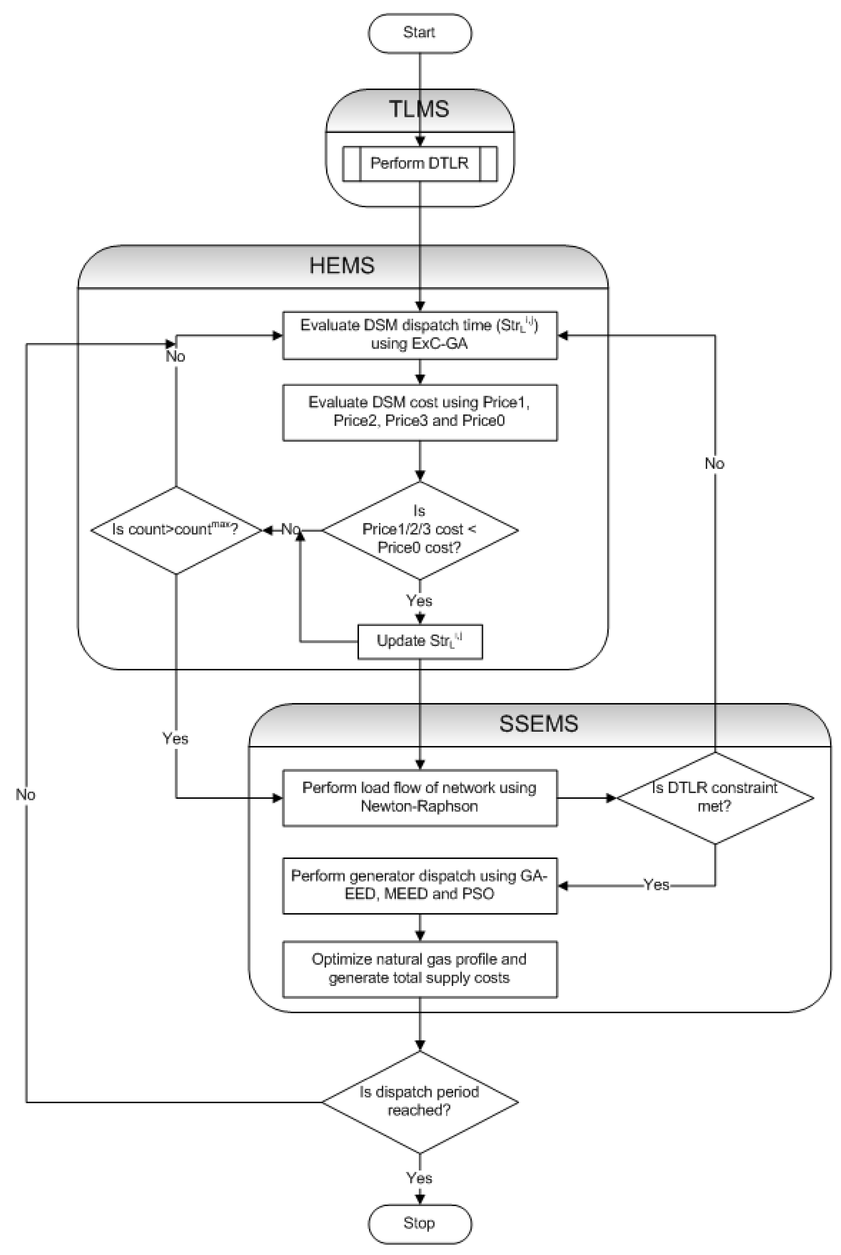
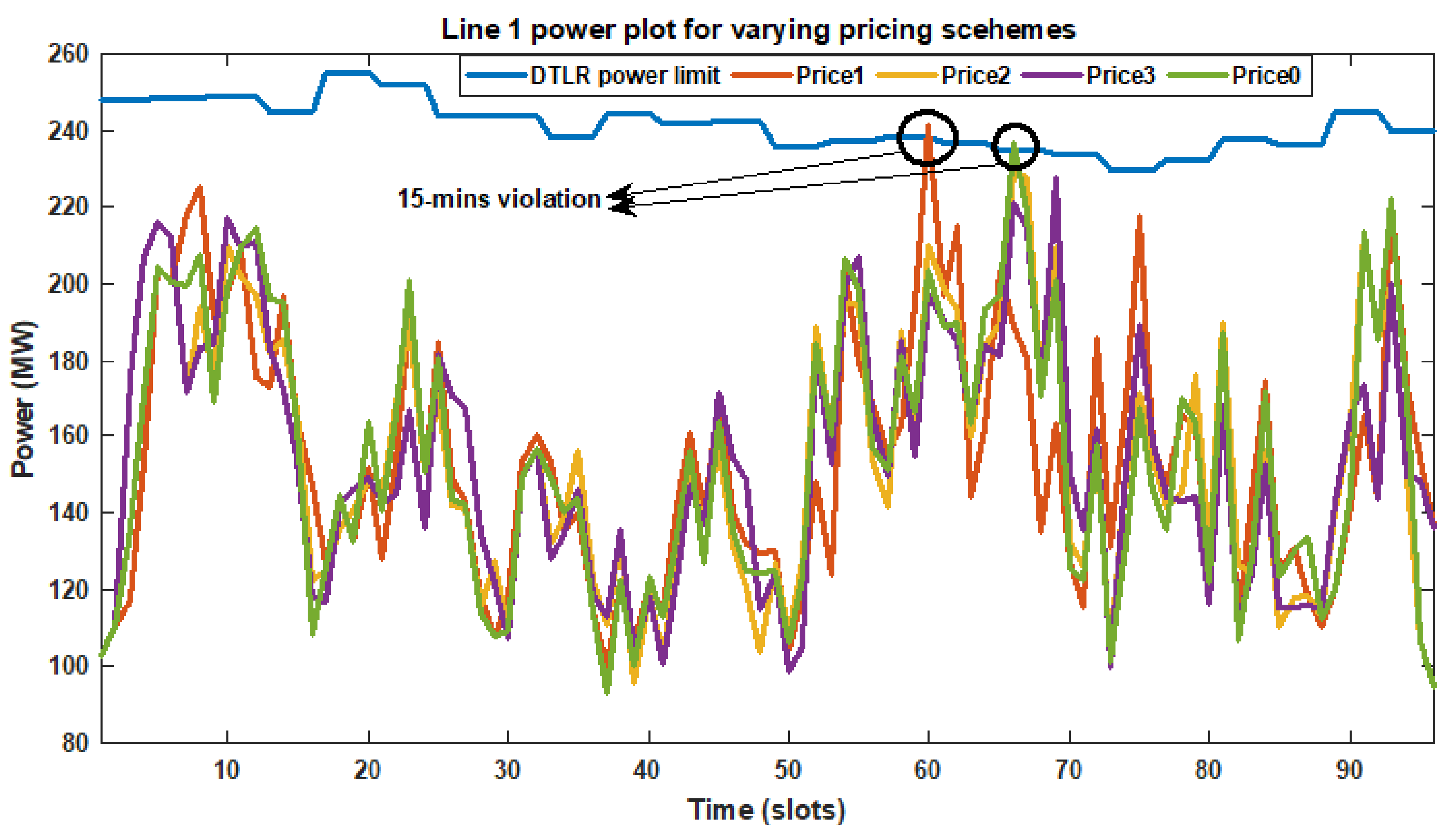
• Reduce consumer electricity bill below available time of use pricing (Price0) (using day ahead dynamic pricing schemes—Price1/Price2/Price3)—HEMS constraint.
• Ensure dynamically computed ampacity limit is not violated by any line—TLMS constraint.
• Reduce operations and emissions cost of the supply side using Price1/Price2/Price3 compared to Price0—SSEMS constraint.

The labelling of the constraints in Figure 1 are as follows:

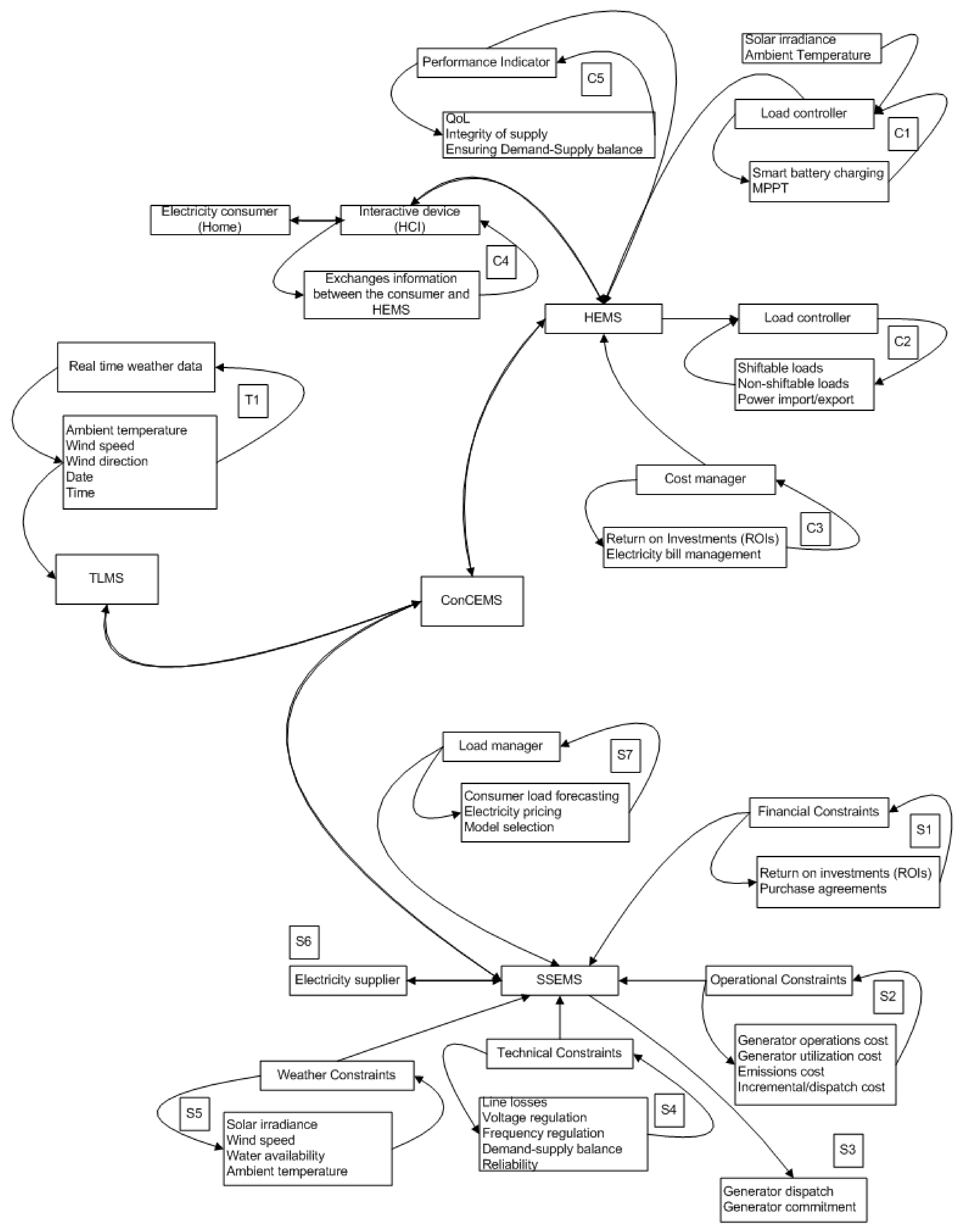
• S1–S7 for SSEMS (i.e., 7 constraints) where S1 is the financial constraint (fuel costs), S2 is the operational constraint (loading limits, reliability), S3 is the generator dispatch/commitment constraint, S4 is the technical constraint (voltage, frequency, var compensation), S5 is the weather constraint, S6 deals with specific constraints from the electricity supplier and S7 is the associated constraint from electricity users on demand response loads.
• C1–C5 for HEMS (i.e., 5 constraints) where C1 deals with battery charging/feed-in-tariff, C2 handles DR loads, C3 manages household expenditure on electricity, C4 updates the household in near-real time on energy usage patterns while C5 ensures household comfort is not compromised.
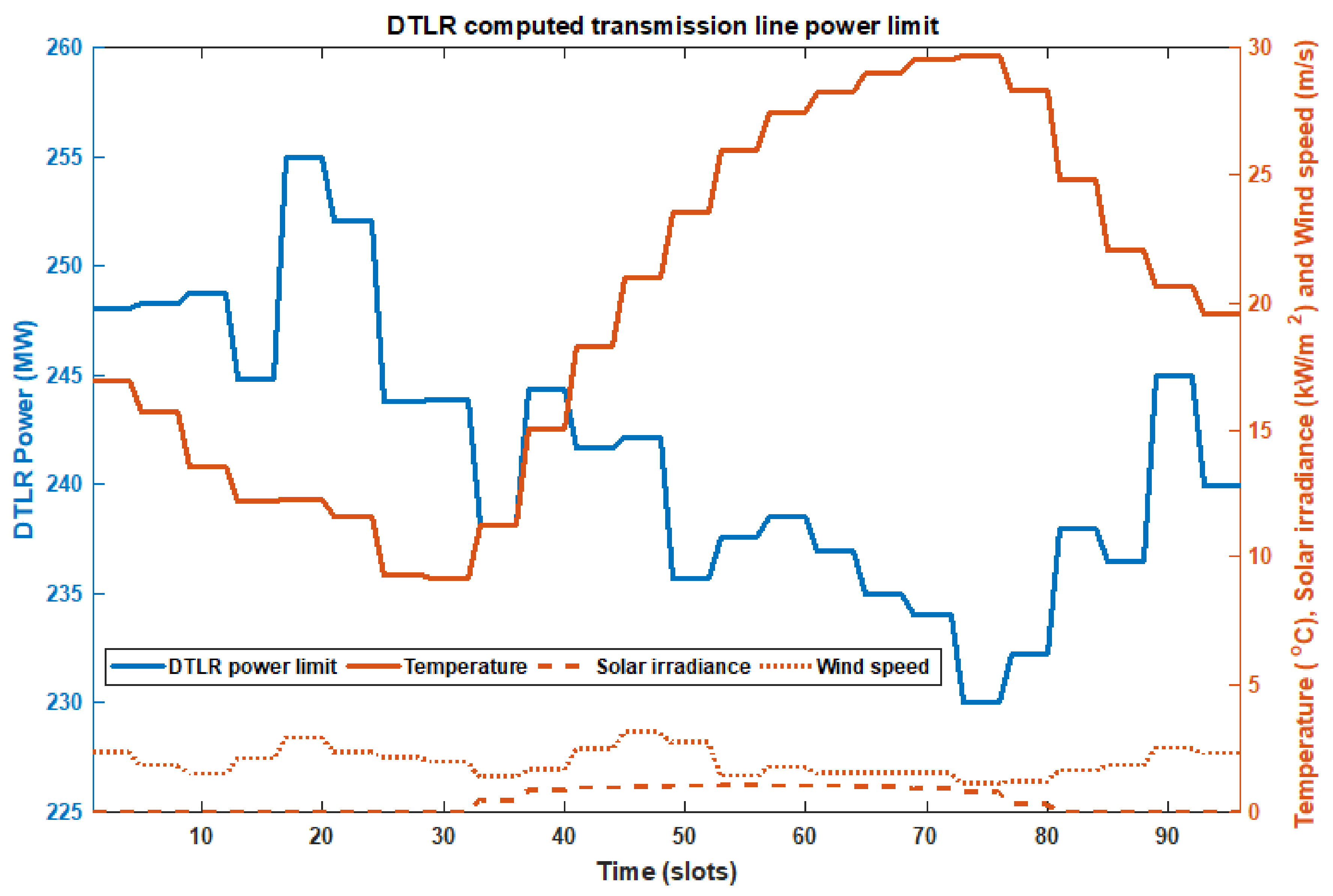
• T1 for TLMS (i.e., 1 constraint) where T1 is the real time weather data (ambient temperature, wind speed and solar irradiance) that affects the computation of transmission line ampacity limits in real-time.

For the purpose of this research,

Table 1. Management systems and their components considered.

HEMS		SSEMS		TLMS
Components	Status	Components	Status	Component	Status
C1	XX	S1	XX	T1	√
C2	√	S2	√
C3	XX	S3	√
C4	√	S4	√ *
C5	XX	S5	XX
		S6	√
		S7	XX

√—component considered; XX—component not considered; *—not all parts of components considered.

highlights which of the constraints have been considered. The rest of this article is organised as follows. Section 2 presents the case study network with the mathematical description of the utilized load flow algorithm. Section 3 presents SSEMS and a mathematical description of its generator dispatch for reduced emissions cost. Section 4 presents TLMS and the description of the DTLR algorithm utilized. HEMS is presented in Section 5 with its objective discussed while the pricing models adopted are presented in Section 6. The results are presented and discussed in Section 7 while policy discussions on the socio-economic and techno-environmental impact of ConCEMS are presented in Section 8. The paper concludes in Section 9.

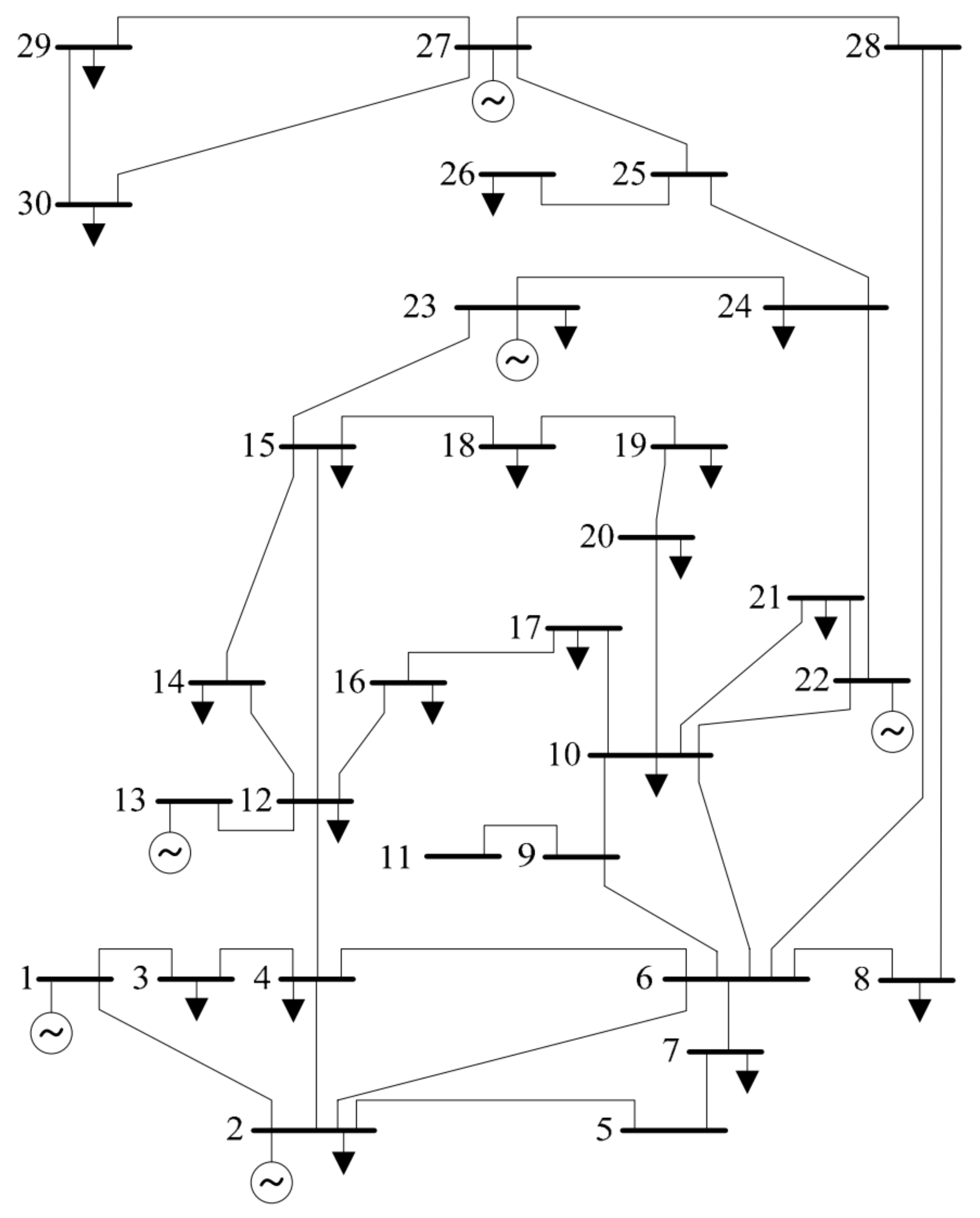
2. Case Study Description

Figure 2 presents the case study network utilized for the application of the proposed ConCEMS while Figure 3 presents the gas network description. The case study network is an IEEE 30-bus network [28] which has been modelled as a closed system with 1 slack power bus (bus 1), 20 load points and 5 generation points. Each load point has both base loads and DR loads. The DR loads for each respective bus is made up of 10 clusters each of households with varying participation of DR loads. The slack power bus has been included to act as a sink/source for excess/deficit power. The test network consists of 41 lines used in moving power across the network. At the slack bus (bus 1), there are 3 generators—2 diesel generators (110 MW each) and 1 natural gas fired thermal generator (50 MW). The description of the demand side management (DSM) capabilities of the various load points is shown in

Table 2. DSM capability of load points.

Bus Number	DSM (MW)
2	39.06
3	72.58
4	13.98
7	51.98
8	61.20
10	132.08
12	21.95
14	14.63
15	17.06
16	7.56
17	19.80
18	7.17
19	14.82
20	32.70
21	37.80
23	7.04
24	18.79
26	27.54
29	5.09
30	24.17

while Figure 4 presents the flow chart of the proposed working principle of ConCEMS. The description of the ConCEMS flowchart is as follows; after the computation of DLTR using hourly weather data, start time of DSM loads, $st{r}_L^{i,j}$ is computed for all participating DSM loads. The cumulative of base load demand and DSM loads for each slot (15 min interval) is then used to optimally determine generation loading based on DTLR constraints for time $t^{\prime }$. Load flow analysis is then done to determine the amount of power supplied from the slack bus and the appropriate costs. In computing $P_T^t$, DTLR could place constraints that would necessitate power import through an alternate line p to meet $P_T^t$ and associated line losses. The computation of $st{r}_L^{i,j}$ using ExC-GA is thus very important in determining the optimal $P_T^t$ that would reduce power supply costs and underutilization of generated power. In addition, the computation of associated supply side costs is followed by the computation of the cost of dispatching the DSM loads using hypothetical day ahead dynamic pricing models (Price1, Price2 and Price3) which are benchmarked with a time of use pricing scheme (Price0). This is to evaluate and determine the best dynamic pricing scheme that will ensure a reduction in DSM load cost, which is the incentive for placing the eventual dispatch of participating DSM loads under direct control by the utility. In computing the associated supply costs for the gas network, ConCEMS aims to generate the least cost for operating the compressors at the various compressor stations that will guarantee the required gas flow rate at the tapoff-point while maintaining the pressure, flow rate and compressibility values within the defined constraints across the length of the pipeline. In minimizing the supply costs for the proposed electricity network, emphasis is placed on the generators in bus 1. This is due to their large size which makes them the major supplier of the bulk load for the test network. The Newton Raphson (NR) method has been adopted in attempting to solve the resulting load flow problem. The modelling of the NR operation is constrained to ensure that convergence is only possible within allowed bus voltage limits. STT and SET for this research have been taken to be 00:00 and 00:00 + 1 day while all dispatch scenarios are carried out a day ahead.

3. SSEMS Description and Modelling

In modelling the SSEMS objective function, $Z_{SSEMS}$, we briefly describe the associated costs at the supply side.

Economic and Environmental Dispatch of Generators

Table 3. Bus 1 associated data for generators.

Bus	Fuel Cost Coefficients *			Real Power Limits (MW)		Type	Emissions Cost ($/MWh)
	a	b	c	Lower	Upper
1	0.005	35	135	20	95	Diesel	100
	0.007	39	110	40	95	Diesel	132
	0.012	23.25	200	30	50	Natural gas	53

*—Incorporates emissions cost.

presents the fuel cost of each generator in bus 1 together with the power limits (lower and upper). Also shown in Table 3 is the emissions cost for each associated generator in bus 1 which has been incorporated into the fuel cost. Algorithm 1 presents the conventional economic dispatch of generators based on incremental cost which has been modified to accommodate emissions cost. The modification results in a modified economic and environmental dispatch (MEED) algorithm. Utilizing the fuel costs of the diesel generators in Table 3, the conventional incremental cost is adjusted to optimally schedule/dispatch the generators at bus 1 for the lowest economic and emissions cost. Another improvement is the compensation for under generation. This is done by optimally allocating the difference in deficit generation among the generators based on their available capacity. The need for this improvement is to reduce the time of computation spent looking for an optimal dispatch profile. Great care is however employed in setting the allowable tolerance level (deficit/surplus generation).

The objective function $Z_{SSEMS}$ is thus defined in Equation (1) as:

$$Z_{SSEMS}=min(O{P}_t^{cost})+min(Z(t))$$

(1)

Subject to:

$$1\le Z_{\alpha }\le 1.6\forall \alpha$$

(2)

$$P^{lo,\alpha }\le P^{\alpha }\le P^{hg,\alpha }\forall \alpha$$

(3)

$$7.5<P{S}_4\le 9.5$$

(4)

$$2.5\le Q_{\alpha }\le 2.7\forall \alpha$$

(5)

$$O{P}_t^{cost}=\sum (Emi{C}_t+F_t^{cost})$$

(6)

$$Z(t)=\sum _{\theta =1}^{\theta =4}{C}^{\theta }(t)$$

(7)

$$Emi{C}_t=\sum _{x=1}^X(E_{x,t}^{cost})$$

(8)

$$E_{x,t}^{cost}=P_{Dx}^t\times w_3$$

(9)

$$Z_{\alpha }=\frac{P{D}_{\alpha }}{P{S}_{\alpha -1}}$$

(10)

$$F_t^{cost}=\sum _{x=1}^X(C_x^{cost,t})$$

(11)

where $\theta$ is a compressor station, $\alpha$ is a pipeline section, $O{P}_t^{cost}$ is the total time t cost of generation by all generators (US$), $Z(t)$ is the total cost of running all compressors at time t (US$), $Z_{\alpha }$ is the pipeline section $\alpha$ compressibility ratio (dimensionless), $P^{lo,\alpha }$ is the pipeline section $\alpha$ low pressure limits (bars), $P^{hg,\alpha }$ is the pipeline section $\alpha$ upper pressure limits (bars), $P^{\alpha }$ is the pipeline section $\alpha$ pressure (bars), $P{S}_4$ is the output pressure (bars), $Q_{\alpha }$ is the pipeline section $\alpha$ gas flow rate (MMSCFD), $Emi{C}_t$ is the total emissions cost at time t (US$), $F_t^{cost}$ is the operations cost at time t (US$), $E_{x,t}^{cost}$ is generator x emissions cost at time t (US$), $P{D}_{\alpha }$ is the discharge pressure (bars) from compressor $\theta$, $P{S}_{\alpha -1}$ is the suction pressure (bars) for compressor $\theta$, $C_x^{cost,t}$ is the cost (US$/MWh) of generating $P_{Dx}^t$ by generator x at time t while every compressor station $\theta$ lies between pipeline sections $\alpha -1$ and $\alpha$ (i.e., $\alpha -1\le \theta <\alpha$). Equation (2) presents the lower and upper compressibility limits for $\alpha$ while Equation (3) describes the lower and upper pressure limits for $\alpha$. The possible range for the final discharge pressure is described in Equation (4) while Equation (5) presents the lower and upper flow rate limits for $\alpha$. The evaluation of $O{P}_t^{cost}$, time t compressor cost, time t total emissions cost, time t emissions cost for generator x, $\alpha$ compressibility ratio and time t operations cost is shown in Equations (6)–(11).

Algorithm 1: Modified incremental generator dispatch.

Input: ${\lambda }_x^t$, ${\lambda }^t$, fuel cost for generators, $P_T^t$, $P_{Dx}^{t-1}$, $P_T^{t-1}$  Output: $P_{Dx}^t$ $\forall x\in X(.)$    Perform normal incremental cost: 1: Compute $P_{Dx}^t$ such that ${\sum }_{x=1}^X(P_{Dx}^t)\simeq P_T^t$ 2: Compute ${\lambda }^t$ such that ${\lambda }_x^t={\lambda }^t$ $\forall x\in X(.)$ 3: Subject to: 4: $P_{Dx}^{min}\le P_{Dx}^t\le P_{Dx}^{max}$$\forall x\in X(.)$ 5: if ($P_T^t\ge P_T^{t-1}$) then 6:  $P_{Dx}^t\ge P_{Dx}^{t-1}$ 7: end if 8: if ($P_T^t<P_T^{t-1}$) then 9:  $P_{Dx}^t\le P_{Dx}^{t-1}$ 10: end if 11: Compute $Emi{C}_t$ and $F_t^{cost}$    Modifications—MEED 12: Set tolerance $w_4$ in MW such that $|P_T^t-{\sum }_{x=1}^X(P_{Dx}^t)| \le w_4$ 13: Vary $P_{Dx}^t$ using $randi$ where $0.75\le randi\le 1$ to evaluate $p_{Dx,modified}^t$ where: 14: $P_{Dx,modified}^t=randi\times P_{Dx}^t$$\forall x\in X(.)$ 15: Update $P_{Dx,modified}^t$ by compensating for $|P_T^t-{\sum }_{x=1}^X(P_{Dx,modified}^t)|$ by computing $dif{f}_x=P_{Dx}^{max}-P_{Dx,modified}^t$ $\forall x\in X(.)$ 16: Set $P_T^{t,modified}={\sum }_{x=1}^X(P_{Dx,modified}^t)$ 17: $P_{Dx,modified}^t=P_{Dx,modified}^t+(\frac{dif{f}_x\times (P_T^t-P_T^{t,modified})}{{\sum }_{x=1}^X(dif{f}_x)})$ 18: Compute $Emi{C}_t^{modified}$, $F_t^{cost,modified}$ and $O{P}_t^{cost,modified}$ 19: if ($O{P}_t^{cost,modified}\le O{P}_t^{cost}$) then 20:  $P_{Dx}^t=P_{Dx,modified}^t$ $\forall x\in X(.)$ 21:  $O{P}_t^{cost}=O{P}_t^{cost,modified}$ 22: end if 23: return$P_{Dx}^t$, $O{P}_t^{cost}$

In improving on the modified incremental generator dispatch (MEED) shown in Algorithm 1, a genetic algorithm-based economic and environmental dispatch (GA-EED) algorithm is developed and presented in Algorithm 2. The purpose for the development of GA-EED is to explore the possibility of eliminating the need for tolerance $w_4$ definition in Algorithm 1 to evolve dispatch options with lower operating costs.

Algorithm 2: Genetic Algorithm Economic and Environmental Dispatch (GA-EED) Algorithm.

Input: fuel cost for generators (Table 3), $P_T^t$, $P_{Dx}^{min}$, $P_{Dx}^{max}$  Output: $P_{Dx}^t$ $\forall x\in X(.)$   Generate binary population matrix for each generator:   Generate $po{p}_x=[dim1\times dim2]$ for each generator x, where $dim1$ is the number of rows (100),   $dim2$ is the number of columns (10) and $po{p}_x$ is a binary matrix.   Perform mutation on $po{p}_x$:  2: Mutation is performed on randomly selected bits of $po{p}_x$ such that   if ($po{p}_x(rr,cc)==1$) then  4:  $po{p}_x(rr,cc)=0$   else  6:  $po{p}_x(rr,cc)=0$   end if   where $1\le rr\le dim1$ and $1\le cc\le dim2$ $\forall rr,cc$   Perform conversion on $po{p}_x$:  8: $po{p}_x$ is converted to its decimal equivalent matrix $po{p}_x^{{}^{\prime }}=[dim1\times 1]$ such that   $po{p}_x^{{}^{\prime }}(rr)=eval(po{p}_x(rr,1:dim2))$,   where $eval$ is a function that converts a binary string into its decimal equivalent.   Perform scaling on $po{p}_x^{{}^{\prime }}$:   Scaling is performed on $po{p}_x^{{}^{\prime }}$ to generate the actual generator values $P_{Dx}^t$ such that   $P_{Dx}^{min}\le P_{Dx}^t\le P_{Dx}^{max}$, where $P_{Dx}^t=\frac{(P_{Dx}^{max}-P_{Dx}^{min})\times po{p}_x^{{}^{\prime }}(rr)}{2^{dim2}-1}+P_{Dx}^{min}$   Perform matching:  10: In matching, a complete allocation $allo{t}_{kk}$ is generated such that if $X=3$,   $allo{t}_{kk}=[po{p}_1^{{}^{\prime }}(r{r}_1), po{p}_2^{{}^{\prime }}(r{r}_2), po{p}_3^{{}^{\prime }}(r{r}_3)]$, where $r{r}_1,r{r}_2,r{r}_3$ are randomly selected rows of $po{p}_1^{{}^{\prime }},po{p}_2^{{}^{\prime }},po{p}_3^{{}^{\prime }}$ respectively, such that $1\le (r{r}_1,r{r}_2,r{r}_3)\le dim1$ and ${\sum }_{x=1}^{X}po{p}_x^{{}^{\prime }}(r{r}_x)\ge P_T^t$   Perform costing and update:   For each $all{o}_{kk}$ generated, an equivalent $cos{t}_{kk}$ is generated where $cos{t}_{kk}$ is the cost of dispatching the generators at bus 1 based on the values in Table 3. In updating the optimal dispatch,  12: if ($cos{t}_{kk}^{new}<cos{t}_{kk}^{old}$) then     $cos{t}_{kk}^{old}=cos{t}_{kk}^{new}$  14:   $allo{t}_{kk}^{old}=allo{t}_{kk}^{new}$     end if  16: $O{P}_t^{cost}=cos{t}_{kk}^{old}$     return $P_{Dx}^t$, $O{P}_t^{cost}$

The degree of accuracy in terms of generating the lowest operational cost for the generators in bus 1 is dependent on the sensitivity factor $s{f}_x$. The sensitivity factor $s{f}_x$ is a measure defined for each generator x as $s{f}_x=\frac{P_{Dx}^{max}-P_{Dx}^{min}}{2^{dim2}-1}$. Thus, as $s{f}_x ⟶0$, the more possible it is to evolve a wider range of possible generation values. However, care must be taken to ensure that $(2^{dim2}-1)\gg (P_{Dx}^{max}-P_{Dx}^{min})$.

Table 4. Generator x sensitivity factor.

x	${\mathit{sf}}_{\mathit{x}}$
1	0.07
2	0.05
3	0.02

presents $s{f}_x$ for each generator at bus 1.

4. TLMS Modelling

The modelling of the ampacity constraints for the transmission lines was done dynamically. That is, real time (1-h interval) weather data was used in dynamically computing the limit of current that could be carried by the transmission line. The computation of the DTLR is done based on the equations described in IEEE std. 738-2006 [29]. From [29], the steady state equations are shown in Equations (12) and (13) as follows:

$$q_c+q_r=q_s+I^{2}R(T_c)$$

(12)

such that

$$I=\sqrt{\frac{q_c+q_r-q_s}{R(T_c)}}$$

(13)

where $q_c$ is heat loss from convection; $q_s$ is the heating effect of the sun; $R(T_c)$ is the AC resistance of the conductor at temperature $T_c$ and I is the conductor current. Out of the 14 inputs that Equations (12) and (13) depend on, five vary in real time–wind speed, wind direction, ambient temperature, time of the day and date. When these values are used without variation, Equations (12) and (13) result in STLR. For this work however, real time hourly data has been used for computing DTLR. The objective function of TLMS, $Z_{TLMS}$ is thus described in (14) as

$$Z_{TLMS}=min(I_{lin{e}_t^p})$$

(14)

subject to

$$I_{lin{e}_t^p}<Am{p}^t$$

(15)

However, an equivalent power limit has been computed based on Equation (15) and utilized in this paper.

5. HEMS Modelling

The HEMS constraint for this research work aims at achieving a reduction in consumers electricity cost for participating DR loads only. In designing the proposed electricity network, base load cost is computed using an incline block tariff (IBT) pricing scheme. However, it is not used in this paper, since emphasis is placed on the participating DR loads. The base pricing scheme utilized in measuring the performance of the dynamic pricing schemes (Price1, Price2 and Price3) is Price0 which is a time of use (TOU) pricing scheme and has a flat rate of $0.105/kWh all through the day except for a $20\%$ increment for the hours between 6 am–8 am and 6 pm–9 pm due to capacity constraints as a result of increased weekdays residential electricity usage during these periods. The participating DR loads are placed on direct load control (DLC) and have their dispatch time varied by the utility within the allowed time range as specified by the electricity consumer. The incentive for allowing the utility some control in varying the dispatch time of participating DR loads is to reduce the cost of these loads by using either of Price1, Price2 or Price3 to offer some minimal electricity cost differentials compared to Price0. In doing so, the utility is able to free up capacity for dispatch of base loads at critical peak demand periods and also minimize the cost of additional generation expansion. The objective function of HEMS $Z_{HEMS}$ is described in Equation (16) as

$$Z_{HEMS}=min(dsm{C}_i^{h_i})$$

(16)

such that

$$dsm{C}_i^{h_i}<tou{C}_i^{h_i}$$

(17)

In achieving Equations (16) and (17), an externally constrained genetic algorithm (ExC-GA) plays a prominent role. The aim of $Z_{HEMS}$ is to ensure that the equivalent cost of electricity using dynamic pricing ($dsm{C}_i^{hi}$) is always less than the equivalent cost of electricity using time of use pricing ($tou{C}_i^{hi}$). This is achieved by comparing the difference $diff=tou{C}_i^{hi}-dsm{C}_i^{hi}$. For $diff<0$, load dispatch is recomputed. Furthermore, for any $dif{f}_{new}>dif{f}_{old}$ and $dif{f}_{old}>0$, then $diff$ is updated to $diff=dif{f}_{new}$. The mathematical modelling of ExC-GA is presented subsequently.

5.1. Externally Controlled Genetic Algorithm

The proposed externally controlled genetic algorithm (ExC-GA) is a modification of the mild intrusive genetic algorithm (MIGA) proposed in [30]. Similar to MIGA, a population matrix $Po{p}_i$ is generated such that the number of rows (dim1) of $po{p}_i$ is $i^{max}$ with the number of columns (dim2) given as 96 (to represent the total number of slots (a slot is a 15 min interval. For a 24 h period, there are 96 slots of 15 min interval each)). The description and working principle of ExC-GA including the modifications incorporated into MIGA is presented subsequently.

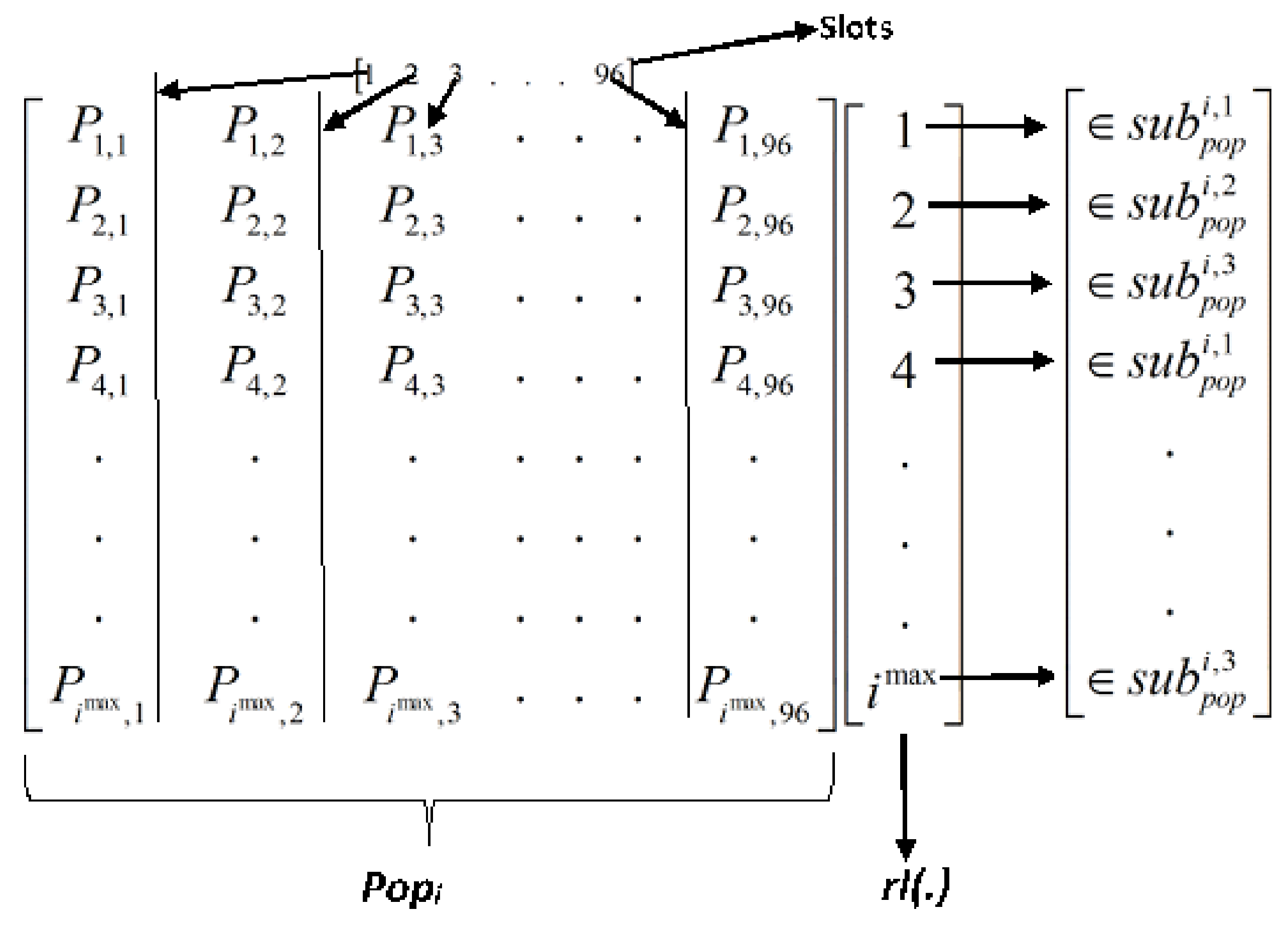
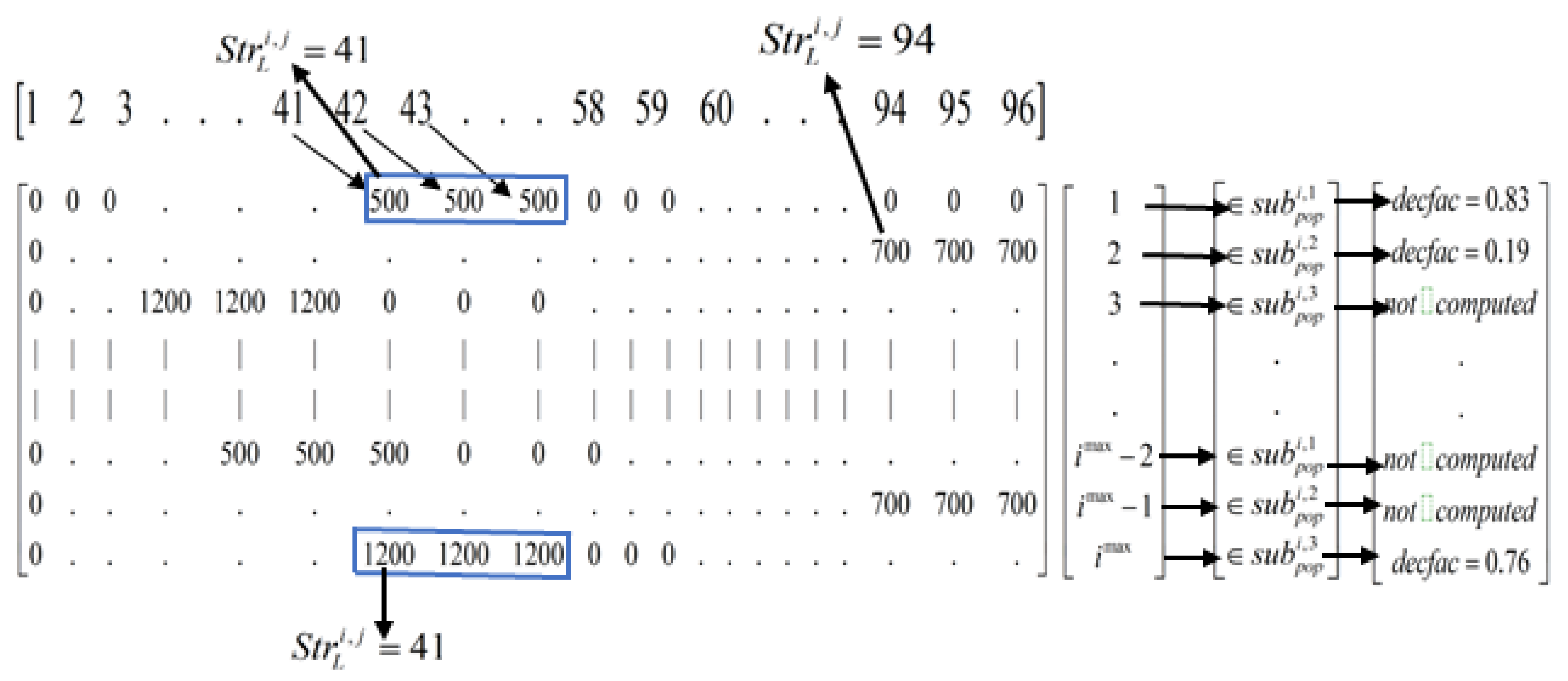
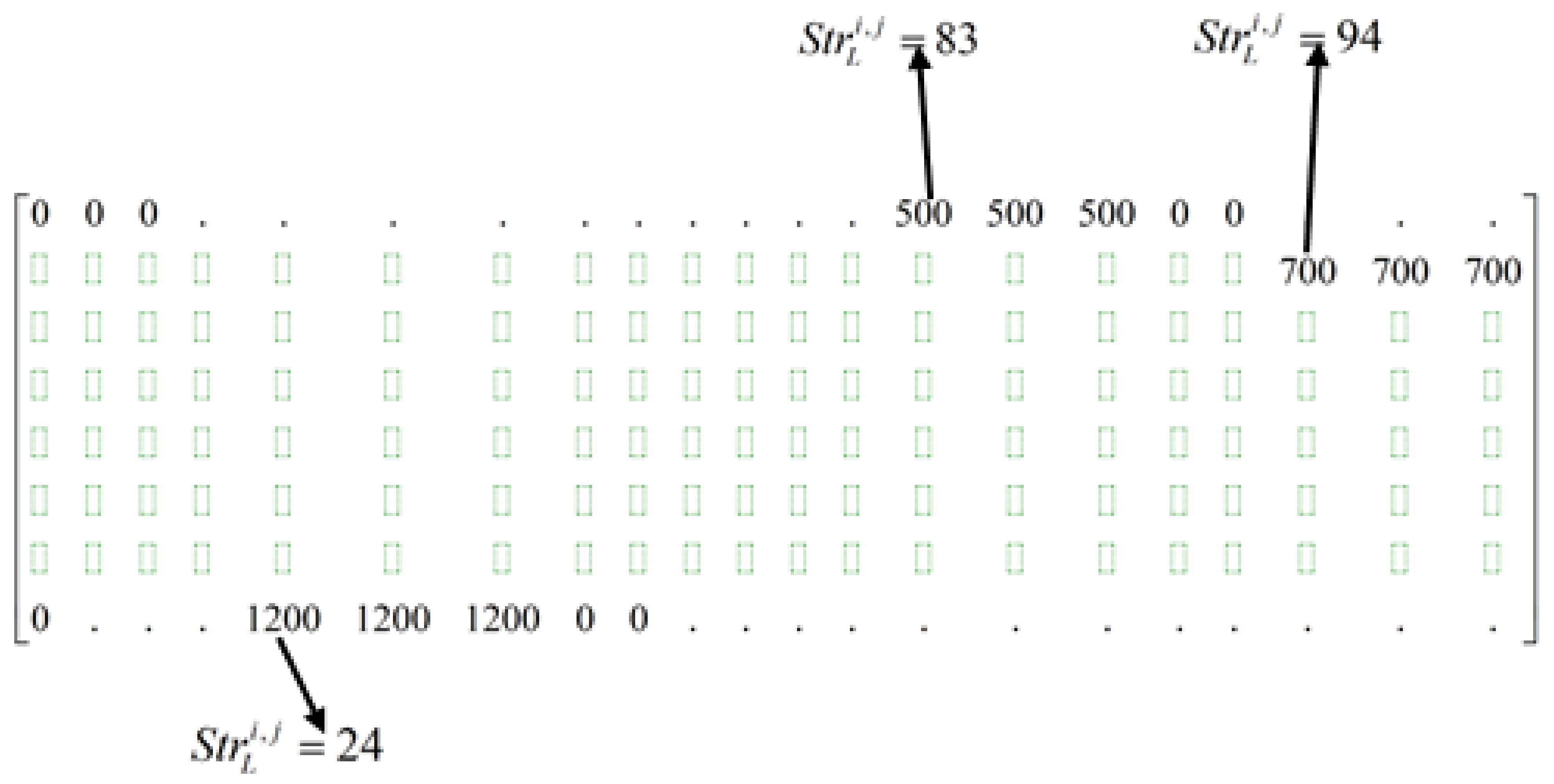
5.1.1. ExC-GA Population Matrix Filling

An initial matrix of dimension $dim1\times dim2$ as shown in Figure 5 is created with all the values initialized to zero (i.e., $\forall P_{1,1}to{P}_{i^{max},96}\in Po{p}_i,P_{1,1}to{P}_{i^{max},96}=0$). Since three DSM loads per household are considered for this research, three sub-populations $su{b}_{pop}^{i,j}$ are created. The sub-populations created are filled with the row index of $po{p}_i$ as follows:

$$su{b}_{pop}^{i,j}=(j,incr,(i^{max}-3+j))$$

(18)

where each $su{b}_{pop}^{i,j}$ is a set of values from j to $(i^{max}-3+j)$ with a successive difference of $incr$ between each element in $su{b}_{pop}^{i,j}$. $\forall \in su{b}_{pop}^{i,j}$, a start point $st{r}_L^{i,j}$ and a stop point $st{p}_L^{i,j}$ are determined as follows:

$$\forall i,andj=1,\left|w^{i,j}\right|=2\Rightarrow 1\le st{r}_L^{i,1}\le 95$$

(19)

$$\forall i,andj=2,\left|w^{i,j}\right|=3\Rightarrow 1\le st{r}_L^{i,2}\le 94$$

(20)

$$\forall i,andj=3,\left|w^{i,j}\right|=5\Rightarrow 1\le st{r}_L^{i,3}\le 92$$

(21)

such that

$$st{p}_L^{i,j}=st{r}_L^{i,j}+w^{i,j}-1\forall st{r}_L^{i,j},st{p}_L^{i,j}\in W(.)$$

(22)

The Equations (19)–(21) assume full DLC in which there are no restrictions for selection of $st{r}_L^{i,j}$. For partial DLC, where the load cluster i specifies a range - intended start time $st{t}_L^{i,j}$ and latest dispatch time $st{d}_L^{i,j}$ for a device j, then $st{t}_L^{i,j}\le st{r}_L^{i,j}\le st{d}_L^{i,j}$.

The incorporation of $-1$ in Equation (22) is to compensate for the inclusion of the start point in the counting of slots/spaces to be filled. The slots/spaces from $st{r}_L^{i,j}$ to $st{p}_L^{i,j}$ are filled with the respective power values as follows:

If $j=1,$ $\forall iDS{M}_j=500$ W, similarly if $j=2,$ $\forall iDS{M}_j=700$ W and if $j=3,$ $\forall iDS{M}_j=1200$ W.

5.1.2. Generation of Violation and Non-Violation Slot Sets—$sta{t}_1^{set}$ and $sta{t}_2^{set}$

The resulting filled population matrix $po{p}_i$ as shown in Figure 6 is then cumulated column wise to obtain $C_i^{DSM}$ for each cluster which is then added to the respective $B{L}_i$ to obtain $C{D}_i$. The resulting $C{D}_i$ is then passed over for load flow operations and generator scheduling operations (see Algorithms 1 and 2) to generate the violation set $sta{t}_1^{set}$ and non-violation set $sta{t}_2^{set}$. The violation set represents all the slots in which ampacity limit was exceeded while the non-violation set represents all the slots in which ampacity limit was not exceeded. The mathematical description of the sets is as follows:

$$sta{t}_1^{set}=(t^{\prime }|amp{a}_p=1)$$

(23)

$$sta{t}_2^{set}=(t^{\prime }|amp{a}_p=0)$$

(24)

Which implies that $\forall sta{t}_1^{set},sta{t}_2^{set}\in W(.)$:

$$\left|sta{t}_1^{set}\right|+\left|sta{t}_2^{set}\right|=96$$

(25)

$$sta{t}_1^{set}\cap sta{t}_2^{set}=\varnothing$$

(26)

$$sta{t}_1^{set}\cup sta{t}_2^{set}=W(.)$$

(27)

The description of $amp{a}_p$ thus implies that if there is a violation of DTLR by any line p during time $t^{\prime }$ simulation, $amp{a}_p=1$, with no violation implying that $amp{a}_p=0$.

5.1.3. $po{p}_i$ Re-Adjustments

The re-adjustments carried out on $po{p}_i$ as shown in Figure 6 is based on the set to which the current $t_L^{\prime }$ belongs to. Thus, $\forall L\in rI(.),$ if $t_L^{\prime }\in sta{t}_1^{set}$, then a decision factor $decfa{c}_{i,L}$ is determined using a random generator, $randi,$ such that:

$$decfa{c}_{i,L}=\{\begin{array}{c}1;ifrandi\ge 0.2\\ 0;ifrandi<0.2\end{array}$$

(28)

Thus, for the row L with $t_L^{\prime }\in sta{t}_1^{set}$ and $decfa{c}_{i,L}\ge 0.2$, then all elements in row L of $po{p}_i$ are initialized to zero. A random start point $t_L^{\prime }\in sta{t}_2^{set}$ is selected as $st{r}_L^{i,j}$ with $st{p}_L^{i,j}$ computed as shown in Equation (22). Next, the slots from $st{r}_L^{i,j}$ to $st{p}_L^{i,j}$ are filled with the respective $DS{M}_j$ as shown in Figure 7 based on the $su{b}_{pop}^{i,j}$ to which L belongs. The resulting $po{p}_i$ is then summed column-wise to compute associated costs and violations if any.

5.2. Comfort Modelling

Given $St{t}_L^{i,j}$ and $St{d}_L^{i,j}$ as the load cluster i intended start time and latest time for dispatch of load j, the comfort limits for these extremes are $C_{max}^i$ and $C_{min}^i$. For any $St{r}_L^{i,j}$ such that $St{t}_L^{i,j}\le St{r}_L^{i,j}\le St{d}_L^{i,j}$, then $C^i$ (for any $St{r}_L^{i,j}$) which is the intermediate comfort and bounded as $C_{min}^i\le C^i\le C_{max}^i$ is defined as shown in Equation (29). For this paper, $C_{max}^i=5$ and $C_{min}^i=3$. The choice of $C_{max}^i$ and $C_{min}^i$ are arbitrary. A comfort scale from 0 to 5 is arbitrarily selected where values $0\le C^i<3$ are assumed to contribute negatively to a consumer. Furthermore, for the research, $C^i\ge 3$ is assumed to be generally accepted. A reason for this assumption is to ensure that the utility in dispatching loads under DLC (full/partial) evolves $St{r}_L^{i,j}$ such that $|St{t}_L^{i,j}-St{r}_L^{i,j}| ⟶0$.

$$C^i={\displaystyle \frac{(C_{max}^i-C_{min}^i)\times (St{r}_L^{i,j}-St{t}_L^{i,j})}{(St{d}_L^{i,j}-St{t}_L^{i,j})}}+C_{min}^{i,j}$$

(29)

6. Pricing

Four pricing schemes are adopted as ‘plug-ins’ in this paper—1 time of use (TOU) pricing (Price0) and 3 dynamic pricing schemes (Price1, Price2 and Price3). The adopted Price0 assumes a flat rate value of US$0.105/kWh across the day with a 20% increase between the hours of 6 am–8 am and 6 pm–9 pm. Price1, Price2 and Price3 are modelled such that their daily average value is US$0.105/kWh with Price1 having peak price between 6 am–8 am, Price2 has peak price between 11 am–1 pm and Price3 has peak price between 6 pm–8 pm. The mathematical description for Price0 is shown in Equation (30) while Equation (31) is the general description for Price1, Price2 and Price3. The pricing models adopted are hypothetical and aim at curtailing demand during their peak periods. The pricing signals are further communicated to consumers within each load cluster a day ahead to enable them schedule $St{t}_L^{i,j}$ for their participating DSM loads. For the purpose of this research, day ahead pricing signals is assumed to be communicated by the utility to electricity consumers via their website. The implication of this is that electricity consumers participating in DLC are assumed to be literate and familiar with information technology (IT) devices for assessing such information. This is similar to the use of the Internet in providing electricity users day ahead pricing information by ComEd in [31].

$$Price0=\{\begin{array}{c}US\$0.126/kWh;6\le t\le 8and18\le t\le 21only\\ US\$0.105/kWh;otherwise\end{array}$$

(30)

$$\sum _{t=1}^{t=24}\frac{Price(t)}{24}=\mathrm{US}\$0.105/\mathrm{kWh}$$

(31)

Motivation for Pricing Methods Selected

The selection of Price0 is to evaluate the ability of ConCEMS in utilizing Price1, Price2 or Price3 to offer potential savings to the consumers and reduced operational costs for the electricity supplier. Furthermore, the varying pricing methods—Price1, Price2 and Price3 have been adopted to compute the extent to which savings (if any) can be offered households participating in DR when compared to Price0 option.

7. Results

The variation of ampacity for the case study network based on DTLR computations is shown for a day in Figure 8. It is seen that power (MW) equivalent of ampcity has been used. Figure 8 shows that power limit computed based on DTLR varies from about 230 MW to about 255 MW per line across the day. The variation of power in Line 1 (between bus 1 and bus 2) for all pricing options is shown in Figure 9. It is observed from Figure 9 that 1 slot (15 min) TLMS violation occurs each for both Price1 and Price0 options with no TLMS violation for Price2 and Price3 options. Assuming 50% STLR (127.5 MW limit) and utilizing Price3, violation is observed for about 74% of the slots. Similarly, for 70% STLR (178.5 MW) and using Price3, violation is observed for 25% of the slots and 9.4% of the slots for 80% STLR (204 MW) and using Price3. ConCEMS thus adopts DTLR and ensures that the transmission network can be maximized in evacuating power without the need for any significant upgrades and without any violations.

Figure 10 presents the various electricity pricing options adopted in this paper—Price1, Price2, Price3 and Price0 across the day While Figure 11 presents the total power supplied from the slack bus (bus 1) across the day. It is observed from Figure 11 that the total power supplied from the slack bus was within the limits set by the generators (lower limit of 90 MW and upper limit of 240 MW).

Figure 12 presents the dispatch of the DR loads under partial DLC for Price1 (DSM1), Price2 (DSM2), Price3 (DSM3) and Price0 (DSM0). It is observed that the DR loads are not able to sufficiently follow their pricing curves due to restraints placed by the users. The restraints in terms of time range within which participating DR loads must be dispatched thus limit the ability of ConCEMS to fully exploit periods of low electricity prices in dispatching participating DR loads. For the DR loads only, Price1 option billed electricity users US$67,243.10 compared with US$66,963.72, US$65,724.62 and US$68,172.06 for Price2, Price3 and Price0 respectively. The implication of this is that the Price3 option achieves a 3.6% reduction in electricity bills for the consumers over Price0 compared to 1.4% and 1.8% savings using Price1 and Price2 respectively. Furthermore, using Price3, load clusters can utilize the additional daily savings of US$2447.44 (over Price0) to purchase additional 19.42 MWh of electricity units at US$0.126/kWh. ConCEMS in utilizing Price3 thus enables consumers extend the usage of owned electrical appliances through savings earned from participating DR loads. ConCEMS also shows that further savings can be achieved for households when DR loads are placed on full DLC (as already shown in [9]), thus highlighting the ability of the proposed ConCEMS to mitigate energy poverty by reducing the energy burden of households.

The utilization of GA-EED and MEED algorithms shown in Algorithm 2 and Algorithm 1 respectively is to highlight the robustness of the ConCEMS framework in incorporating varying stochastic and classical optimization schemes in minimizing the associated operations and environmental costs for the supply side. However, in benchmarking the results obtained using GA-EED and MEED algorithms, a standard particle swarm optimization (PSO) algorithm is also utilized to solve a single dispatch problem with the results obtained compared with those from the proposed algorithms (GA-EED and MEED) in this paper.

Table 5. GA-EED, MEED and PSO dispatch profile for 225 MW.

Method	Tries	Cost (US$)	Time (S)	Surplus Generation (MW)	Dispatch Profile (MW)
					Gen 1	Gen 2	Gen 3
GA-EED	1	8194.8	3.6209	0.19	94.63	81.4	49.16
	2	8219.67	1.6099	0.03	85.62	89.78	49.63
	3	8216.61	2.685	0.45	91.11	84.95	49.39
	4	8216.51	3.072	0.48	89.5	86.08	49.9
	5	8272.43	5.945	0.01	89.94	90	45.07
Average		8224	3.39	0.23	90.16	86.44	48.63
PSO	1	8414.81	8.7653	6.04	95	86.04	50
	2	8414.81	8.7563	6.04	95	86.04	50
	3	8414.81	8.9277	6.04	95	86.04	50
	4	8414.81	8.8108	6.04	95	86.04	50
	5	8414.81	8.8422	6.04	95	86.04	50
Average		8414.81	8.8205	6.04	95	86.04	50
MEED	1	8237.67	0.2744	0	80	95	50
	2	8238.77	0.2944	0.03	80.03	95	50
	3	8238.74	0.2784	0.03	80.03	95	50
	4	8240.13	0.2676	0.07	80.07	95	50
	5	8237.67	0.3026	0	80	95	50
Average		8238.6	0.28	0.03	80.03	95	50

Gen—Generator.

presents the values obtained for each method over five trials which is then averaged. It is observed from Table 5 that the fastest algorithm is the MEED algorithm which achieves an average run time of 0.28 s compared to 3.37 s and 8.82 s for GA-EED and PSO respectively. The comparison of the total daily simulation time for Price1, Price2, Price3 and Price0 using GA-EED shows that Price1 achieves a simulation time of 14.23 s, Price2 achieves a simulation time of 13.80 s, Price3 achieves a simulation time of 11.66 s while Price0 achieves a simulation time of 13.61 s. However, GA-EED achieves the lowest operational cost of US$8224.00 compared to US$8238.60 and US$8414.81 for MEED algorithm and PSO respectively. In terms of surplus generation, MEED algorithm generates 100.01% of the required demand compared to 100.10% and 102.68% of the required demand by GA-EED and PSO.

Table 6. Supply cost (US$) for various optimisation algorithms.

Option	Optimisation Algorithms			Violations	Duration (Slots)
	GA-EED	MEED	PSO
Price1	531937.93	543211.98	532200.8	1	1
Price2	532183.92	543636.61	533491	0	- ${}^{\mathrm{a}}$
Price3	531807.8	542361.61	533032.2	0	- ${}^{\mathrm{a}}$
Price0	532717.88	544211.98	533880.3	1	1

a—Implies not applicable since no violation occurs.

further presents the supply cost (the supply cost computed and shown in Table 6 incorporates the compressor cost) for the various pricing options (Price1, Price2, Price3 and Price0) and different optimisation algorithms (MEED, GA-EED and PSO). Similar to Table 5, GA-EED offers the lowest operations cost for supply side for all pricing options compared to PSO and MEED with Price3 offering the lowest cost of US$531,807.80 and US$542,361.61 for GA-EED and MEED respectively, and Price1 offering the lowest supply cost of US$532,200.80 for PSO. The utilization of the compressors at the outlet point for optimal flow of gas at reduced compressor usage cost for Price3 using GA-EED is shown in Figure 13. Also depicted in Figure 13 is the suction and discharge pressure for each slot (15 min interval) at the outlet/tapoff-point which is maintained within constrained limits.

A further implication of ConCEMS to the utility is that ConCEMS enables the utility reduce the associated costs of expanding generation capacity to meet demand. With ConCEMS, flexible loads can be effectively dispatched at reduced peak demand and with increased capacity utilization. Furthermore, increased flexibility in the network through DLC (full or partial) provides the utility with advanced information for system operation and planning, scheduling maintenance and dealing with outages. With increased flexible loads under DLC, the utility is able to respond better in establishing optimal grid operation in the event of faults or loss of a generating unit.

Table 7. Dispatch time $St{r}_L^{i,j}$ for DR loads of various pricing options on bus 2.

Bus	Cluster	${\mathit{Stt}}_{\mathit{L}}^{\mathit{i},\mathit{j}}$	${\mathit{Std}}_{\mathit{L}}^{\mathit{i},\mathit{j}}$	Price1	Price2	Price3	Price0
2	1	1	5	5	5	5	5
	2	89	93	91	90	90	91
	3	54	74	59	59	59	59
	4	44	64	64	64	64	64
	5	2	6	2	2	2	2
	6	46	66	52	52	52	52
	7	69	89	78	73	73	78
	8	40	84	76	76	76	76
	9	3	7	4	3	3	4
	10	4	48	14	14	9	9

presents $St{r}_L^{i,j}$ for each cluster on bus 2 and for the various pricing options while

Table 8. Comfort $C^i$ for each pricing option for $St{r}_L^{i,j}$ on bus 2.

Bus	Cluster	Price1	Price2	Price3	Price0
2	1	3	3	3	3
	2	4	4.5	4.5	4
	3	4.5	4.5	4.5	4.5
	4	3	3	3	3
	5	5	5	5	5
	6	4.4	4.4	4.4	4.4
	7	4.1	4.6	4.6	4.1
	8	3.36	3.36	3.36	3.36
	9	4.5	5	5	4.5
	10	4.55	4.55	4.77	4.77
	Average	4.04	4.19	4.21	4.06

presents the computed comfort $C^i$ for each cluster which has been evaluated using Equation (29). It is observed from Table 8 that Price3 option offers the highest comfort of 4.21 followed by Price2 (4.19), Price0 (4.06) and Price1 (4.04). In summary therefore, Price3 utilizing GA-EED meets all the requirements by reducing the electricity cost for participating DR loads and supply cost of the supply side without violating the transmission line power limit constraint. This is shown in

Table 9. Performance summary for various dynamic pricing options using GA-EED and MEED.

	GA-EED			MEED			${\mathit{C}}^{\mathit{i}}$
	HEMS	SSEMS	TLMS	HEMS	SSEMS	TLMS
Price1	√	√	X	√	√b	X	X
Price2	√	√	√	√	√	√	√
Price3	√b	√b	√	√b	√	√	√b

b—Best option.

where Price3 with GA-EED in addition to meeting HEMS, TLMS and SSEMS constraints further improves on the comfort of participating households by ensuring that $St{r}_L^{i,j}$ strives to be close to $St{t}_L^{i,j}$.

Table 10. Further benchmarking of GA-EED from [32].

Number	Name of Function	Range	D	Type	Minimum	Minimum (GA-EED)
1	Beale	[−4.5, 4.5]	2	UN	0	3.12E-05
2	Matyas	[−10, 10]	2	UN	0	3.82E-06
3	Bohachevskyl	[−100, 100]	2	MS	0	2.53E-04
4	Bohachevsky2	[−100, 100]	2	MN	0	6.99E-04
5	Bohachevsky3	[−100, 100]	2	MN	0	7.04E-04
6	Booth	[−10, 10]	2	MS	0	3.45E-05
7	Six Hump Camel Back	[−5, 5]	2	MN	−1.03163	−1.03160
8	Easom	[−100, 100]	2	UN	−1	−0.99647
9	Schaffer	[−100, 100]	2	MN	0	1.22E-07

D—Dimensions; U—unimodal; N—non-seperable; M—multimodal; S—seperable.

presents the results obtained from further benchmarking of GA-EED against nine standard benchmarking functions from [32]. The performance of GA-EED in matching the exact solutions is also observed.

8. Policy Discussions

ConCEMS pioneers the full synergy of HEMS, TLMS and SSEMS by extending the model presented in [9]. As a smart grid architecture that depends on an advanced metering infrastructure (AMI), ConCEMS has benefits extending from the socio-economic to the techno-environmental aspects of society which are subsequently discussed.

8.1. Policy Discussions on the Impact of ConCEMS on the Socio-Economic Aspect of Society

A growing concern in the global south is the issue of energy poverty which presents on two frontiers—access and mobility (ability to transit from a lower energy level to a higher energy level). Furthermore, in the works of [33,34], declining electricity consumption (per capita) has been highlighted for Nigeria and South Africa respectively. A prominent reason for this has been increasing electricity tariff which has resulted in the increasing use of alternative energy sources. Furthermore, [34] has highlighted the direct link between energy poverty and economic poverty. The increasing tariffs by Eskom (Eskom is the electricity utility company for South Africa generating over 90% of electricity consumed in South Africa and 45% of electricity consumed in Africa [33]) are intended to recoup electricity network expansion costs especially in building new generation plants and improving the transmission network to prevent a repeat of the power crisis of 2008. However, according to [33], there is the possibility of planned supply capacity exceeding demand forecasts by over 500% due to declining consumption of electricity. ConCEMS obviates the need for unnecessary upgrades by ensuring that flexible consumers (DR loads) are well incorporated into the overall system mix to act as deferrable loads that offer some flexibility to the system operator in ensuring demand-supply balance. Incorporating dynamic pricing schemes (Price1, Price2 and Price3), the utility is able to guarantee households a reduction in their electricity bills. This reduced expenditure on electricity offers households the possibility of either increasing consumption of more electricity or utilizing the savings accrued on other activities capable of improving their quality of life (QoL). Overall, with increasing participation of more households in DR, the utility is able to save on expansion costs and also utilize effectively renewable energy sources (RES) by dispatching DR loads to times of high availability of RES.

8.2. Policy Discussion on the Techno-Environmental Impact of ConCEMS

The increasing complexity of electricity network raises concerns as to the ability of evolving electricity networks to handle the bi-directional flow of energy with increasing prosumers (consumers who also produce electricity through on-site mini generation schemes) and DR loads. Furthermore, the increasing participation of RES and their stochasticity raises issues of reactive power compensation and grid stability. ConCEMS in ensuring that the technical constraints are met utilizes increasing DR loads in balancing the grid. However, the extent of flexibility in ensuring grid stability through the utilization of flexible loads is based on the time allowance given the utility by the consumers. In [9], the proposed energy management system minimized peak DSM window by over 63% with an overall capacity utilization of 87.92% when the utility was fully in control of determining the start and eventual dispatch time of participating DR loads. Worldwide, there have been growing concerns to the insidious effect of fossil-based electricity generation on climate. The incorporation of GA-EED optimizes the dispatch of the participating generators to minimize the overall cost (operations and environmental). Furthermore, the increasing participation of flexible loads implies that ConCEMS in optimizing their dispatch time to periods of availability of RES can maximize the usage of available RES thus reducing environmental costs associated with conventional generation schemes.

8.3. Summary and Applicability of ConCEMS

ConCEMS has been presented as a tool capable of mitigating energy poverty and minimizing grid expansion. This is mostly important especially for developing economies (sub-Saharan Africa, SSA) where socially just power systems are required in order to facilitate the promotion of access to electricity without marginalizing the poor [35]. Considering the fact that ConCEMS integrates every aspect of the electricity network and achieves savings, the following arise:

1

The utilization of DTLR reduces transmission expansion costs which leads to stabilization of electricity tariffs for electricity users. In South Africa, Eskom’s electricity tariff increment (to recoup supply capacity costs) has resulted in declining electricity consumption [33]. With stabilized electricity costs, the energy burden of households is minimized.

2

The ability of ConCEMS to guarantee savings for households participating in DR (for participation of 3 devices only) shows that more savings could be accrued when more energy consuming devices especially heating, ventilation and cooling (HVAC) devices are considered. A reduction in electricity bills for households (whose electricity bills have already been stabilized due to the incorporation of DTLR) leads to even further reduction in households energy burden.

3

ConCEMS has shown that flexible loads offer the utility great flexibility which is capable of minimizing supply capacity expansion. With greater flexibility offered the utility especially through greater participation in DR and DLC, the utility is able to minimize expansion costs and reduce spinning reserves without compromising on grid constraints (investigated in [33]). The implication of this implies that electricity tariffs remain stabilized which leads to minimized energy burden of households.

4

ConCEMS also offers a great platform for increasing the exploitation of renewable energy sources (RES) thereby leading to a reduction in emissions. With greater flexibility offered the utility in terms of controllable loads, the utility is able to effectively dispatch participating DSM loads to periods of availability of RES.

ConCEMS depends on an integrated electricity network the core of which is an advanced metering infrastructure (AMI) and a robust transmission network to guarantee its effective deployment and utilisation. For SSA, the need for infrastructure upgrades coupled with the growing calls for reduction in emissions presents an opportunity for SSA countries to develop grids that promote integration across the entire electricity chain.

9. Conclusions

ConCEMS has been presented and evaluated for an IEEE 30-bus network with an externally constrained genetic algorithm (ExC-GA) also designed and used in demand response load dispatch. Two economic and environmental dispatch algorithms for generators on bus 1—GA-EED and MEED have also been developed, applied and benchmarked using a standard PSO. In evaluating the ability of ConCEMS in meeting the objectives of HEMS, TLMS and SSEMS, three dynamic pricing schemes (Price1, Price2 and Price3) have been proposed and benchmarked with a time of use pricing scheme (Price0). Price3 has been found to reduce both the electricity cost of participating DR loads and the operational costs of the supply side without violating the transmission line power limit. Furthermore, Price3 with GA-EED has been found to ensure that the eventual dispatch time ($St{r}_L^{i,j}$) of participating DR loads is close to the intended start time ($St{t}_L^{i,j}$) of the loads by the users. This has been verified by the high value of comfort ($C^i$) which is about $0.84C_{max}^i$. Policy discussions on the impact of ConCEMS on the socio-economic and techno-environmental aspect of society have also been presented to show that ConCEMS is also a capable tool in mitigating energy poverty by minimizing tariff increment through the maximized use of RES and available supply capacity, thus minimizing capacity upgrades. This has been elaborated by the ability of ConCEMS to offer the utility flexibility in varying the dispatch time of participating DR loads to reduce peak demand and maximize transmission network and supply capacity. However, it must be highlighted that ConCEMS is limited based on the degree of participation of DR loads and flexibility (in terms of dispatch time) offered the utility by the consumers. With strict time frames for load dispatch, partial DLC and the need to ensure that $|St{t}_L^{i,j}-St{r}_L^{i,j}| ⟶0$, ConCEMS offers the utility a limited window of flexibility. However, when consumers participate in full DLC, ConCEMS is able to offer the utility higher flexibility in maximizing benefits for both the consumer and the supplier. Results obtained thus show that the extent of performance of ConCEMS in meeting the objectives of HEMS, SSEMS and TLMS is determined by the nature of the pricing profile selected and the size and flexibility of participating DR loads. In terms of general applicability, the proposed ConCEMS can be applied widely for both industrial and household DR scheduling optimisation purposes since the pricing schemes are ’plug-ins’. Furthermore, the proposed GA-EED has been benchmarked and found to outperform the contemporary MEED and conventional PSO in achieving the best results. ExC-GA has also been seen to offer $St{r}_L^{i,j}$ that ensure a high comfort level for consumers while guaranteeing a reduction in electricity cost for consumers.

10. Future Work

Considering the ability of ConCEMS to provide some flexibility to the utility especially in reducing peak demand and increasing utilization of the transmission network through DTLR, future research would aim at exploiting the ability of ConCEMS to still guarantee reduced electricity bills for consumers and optimal grid operation in the event of faults. Future work thus aims at determining the limit of ConCEMS to guaranteeing the objectives of HEMS, SSEMS and TLMS under dynamic network faults.

References

1. Martinez-Mares, A.; Fuerte-Esquivel, C.R. A Unified Gas and Power Flow Analysis in Natural Gas and Electricity Coupled Networks. IEEE Trans. Power Syst. 2012, 27, 2156–2166. [Google Scholar] [CrossRef]
2. Sun, Y.; Song, H.; Jara, A.J.; Bie, R. Internet of Things and Big Data Analytics for Smart and Connected Communities. IEEE Access 2016, 4, 766–773. [Google Scholar] [CrossRef]
3. Ronellenfitsch, H.; Manik, D.; Hörsch, J.; Brown, T.; Witthaut, D. Dual theory of transmission line outages. IEEE Trans. Power Syst. 2017, 32, 4060–4068. [Google Scholar] [CrossRef]
4. Cong, Y.; Regulski, P.; Wall, P.; Osborne, M.; Terzija, V. On the Use of Dynamic Thermal-Line Ratings for Improving Operational Tripping Schemes. IEEE Trans. Smart Grid 2016, 31, 1891–1900. [Google Scholar] [CrossRef]
5. Chaichana, A.; Syed, M.H.; Burt, G.M. Vulnerability mitigation of transmission line outages using demand response approach with distribution factors. In Proceedings of the 2016 IEEE 16th International Conference on Environment and Electrical Engineering (EEEIC), Florence, Italy, 7–10 June 2016; pp. 1–6. [Google Scholar]
6. Ji, G.; Wu, W.; Zhang, B. Robust generation maintenance scheduling considering wind power and forced outages. IET Renew. Power Gener. 2016, 10, 634–641. [Google Scholar] [CrossRef]
7. Koval, D.O.; Chowdhury, A.A. Assessment of Transmission-Line Common-Mode, Station-Originated, and Fault-Type Forced-Outage Rates. IEEE Trans. Ind. Appl. 2010, 46, 313–318. [Google Scholar] [CrossRef]
8. Anderson, C.L.; Davison, M. A Hybrid System-Econometric Model for Electricity Spot Prices: Considering Spike Sensitivity to Forced Outage Distributions. IEEE Trans. Power Syst. 2008, 23, 927–937. [Google Scholar] [CrossRef]
9. Monyei, C.G.; Adewumi, A.O. Integration of demand side and supply side energy management resources for optimal scheduling of demand response loads South Africa in focus. Electr. Power Syst. Res. 2018, 158, 92–104. [Google Scholar] [CrossRef]
10. Mwale, S.J.T.; Davidson, I.E. Power deficits and outage planning in South Africa. In Proceedings of the 2nd International Symposium on Energy Challenges and Mechanics, Aberdeen, UK, 19–21 August 2014. [Google Scholar]
11. Mwale, S.J.T.; Davidson, I.E. SADC Power Grid Reliability—A Steady-state Contingency Analysis and Strategic HVDC Interconnections Using the N-1 Criterion. In Proceedings of the 2nd International Symposium on Energy Challenges and Mechanics, Aberdeen, UK, 19–21 August 2014. [Google Scholar]
12. Karunanithi, K.; Saravanan, S.; Prabakar, B.R.; Kannan, S.; Thangaraj, C. Integration of Demand and Supply Side Management strategies in Generation Expansion Planning. Renew. Sustain. Energy Rev. 2017, 73, 966–982. [Google Scholar] [CrossRef]
13. Pratt, A.; Krishnamurthy, D.; Ruth, M.; Wu, H.; Lunacek, M.; Vaynshenk, P. Transactive Home Energy Management Systems: The Impact of Their Proliferation on the Electric Grid. IEEE Electrification Mag. 2016, 4, 8–14. [Google Scholar] [CrossRef]
14. Althaher, S.; Mancarella, P.; Mutale, J. Automated Demand Response From Home Energy Management System Under Dynamic Pricing and Power and Comfort Constraints. IEEE Trans. Smart Grid 2015, 6, 1874–1883. [Google Scholar] [CrossRef]
15. Zhang, D.; Li, S.; Sun, M.; O’Neill, Z. An Optimal and Learning-Based Demand Response and Home Energy Management System. IEEE Trans. Smart Grid 2015, 7, 1790–1801. [Google Scholar] [CrossRef]
16. Crdenas, J.J.; Romeral, L.; Garcia, A.; Andrade, F. Load forecasting framework of electricity consumptions for an Intelligent Energy Management System in the user-side. Expert Syst. Appl. 2012, 39, 5557–5565. [Google Scholar] [CrossRef]
17. Camacho, R.; Carreira, P.; Lynce, I.; Resendes, S. An ontology-based approach to conflict resolution in Home and Building Automation Systems. Expert Syst. Appl. 2014, 41, 6161–6173. [Google Scholar] [CrossRef]
18. Martinez-Pabon, M.; Eveleigh, T.; Tanju, B. Optimizing residential energy management using an autonomous scheduler system. Expert Syst. Appl. 2018, 96, 373–387. [Google Scholar] [CrossRef]
19. Batista, A.C.; Batista, L.S. Demand Side Management using a multi-criteria -constraint based exact approach. Expert Syst. Appl. 2018, 99, 180–192. [Google Scholar] [CrossRef]
20. Gunda, J.; Djokic, S. Coordinated control of generation and demand for improved management of security constraints. In Proceedings of the 2016 IEEE PES Innovative Smart Grid Technologies Conference Europe (ISGT-Europe), Ljubljana, Slovenia, 9–12 October 2016; pp. 1–6. [Google Scholar]
21. Ramachandran, B.; Srivastava, S.K.; Cartes, D.A. Intelligent power management in micro grids with EV penetration. Expert Syst. Appl. 2013, 40, 6631–6640. [Google Scholar] [CrossRef]
22. Alonso, M.; Amaris, H.; Alvarez-Ortega, C. Integration of renewable energy sources in smart grids by means of evolutionary optimization algorithms. Expert Syst. Appl. 2012, 39, 5513–5522. [Google Scholar] [CrossRef]
23. Chakraborty, S.; Nakamura, S.; Okabe, T. Real-time energy exchange strategy of optimally cooperative microgrids for scale-flexible distribution system. Expert Syst. Appl. 2015, 42, 4643–4652. [Google Scholar] [CrossRef]
24. Van Beuzekom, I.; Mazairac, L.A.J.; Gibescu, M.; Slootweg, J.G. Optimal design and operation of an integrated multi-energy system for smart cities. In Proceedings of the 2016 IEEE International Energy Conference (ENERGYCON), Leuven, Belgium, 4–8 April 2016; pp. 1–7. [Google Scholar]
25. Bai, L.; Li, F.; Jiang, T.; Jia, H. Robust Scheduling for Wind Integrated Energy Systems Considering Gas Pipeline and Power Transmission Contingencies. IEEE Trans. Power Systems 2017, 32, 1582–1584. [Google Scholar] [CrossRef]
26. Cartes, D.; Ordonez, D.; Harrington, J.; Cox, D.; Meeker, R. Novel Integrated Energy Systems and Control Methods with Economic Analysis for Integrated Community Based Energy Systems. In Proceedings of the 2007 IEEE Power Engineering Society General Meeting, Tampa, FL, USA, 24–28 June 2007; pp. 1–6. [Google Scholar]
27. Hajimiragha, A.; Canizares, C.; Fowler, M.; Geidl, M.; Andersson, G. Optimal Energy Flow of integrated energy systems with hydrogen economy considerations. In Proceedings of the 2007 iREP Symposium—Bulk Power System Dynamics and Control VII. Revitalizing Operational Reliability, Charleston, SC, USA, 19–24 August 2007; pp. 1–11. [Google Scholar]
28. Single Line Diagram of the IEEE 30-Bus Test System. Available online: http://een.iust.ac.ir/profs/Jadid/SCPM.pdf (accessed on 17 January 2018).
29. IEEE. IEEE Standard for Calculating the Current-Temperature Relationship of Bare Overhead Conductors; IEEE Std. 738-2012 (Revision of IEEE Std 738-2006—Incorporates IEEE Std 738-2012 Cor 1-2013); IEEE Standards Association: New York, NY, USA, 2013. [Google Scholar]
30. Monyei, C.G.; Adewumi, A.O.; Obolo, M.O. Oil Well Characterization and Artificial Gas Lift Optimization Using Neural Networks Combined with Genetic Algorithm. Discret. Dyn. Nat. Soc. 2014, 2014, 289239. [Google Scholar] [CrossRef]
31. ComEd. Available online: https://hourlypricing.comed.com/live-prices/ (accessed on 20 March 2018).
32. Cheng, M.-Y.; Prayogo, D. Symbiotic Organisms Search: A new metaheuristic optimization algorithm. Comput. Struct. 2014, 139, 98–112. [Google Scholar] [CrossRef]
33. Monyei, C.G.; Adewumi, A.O. Demand Side Management potentials for mitigating energy poverty in South Africa. Energy Policy 2017, 111, 298–311. [Google Scholar] [CrossRef]
34. Monyei, C.G.; Adewumi, A.O.; Obolo, M.O.; Sajou, B. Nigeria’s energy poverty: Insights and implications for smart policies and framework towards a smart Nigeria electricity network. Renew. Sustain. Energy Rev. 2018, 81, 1582–1601. [Google Scholar] [CrossRef]
35. Welsch, M.; Bazilian, M.; Howells, M.; Divan, D.; Elzinga, D.; Strbac, G.; Jones, L.; Keane, A.; Gielen, D.; Murthy Balijepalli, V.S.K.; et al. Smart and Just Grids for sub-Saharan Africa: Exploring options. Renew. Sustain. Energy Rev. 2013, 20, 336–352. [Google Scholar] [CrossRef]
Figure 1. ConCEMS conceptual design.
Energies 11 01038 g001
Figure 2. IEEE 30-bus electricity network [28].
Energies 11 01038 g002
Figure 3. Hypothetical gas network.
Energies 11 01038 g003
Figure 4. Flowchart of ConCEMS.
Energies 11 01038 g004
Figure 5. p o p i with its description.
Energies 11 01038 g005
Figure 6. D S M j load allocation in p o p i based on s t r L i , j .
Energies 11 01038 g006
Figure 7. Re-computation of s t r L i , j based on s t a t 1 s e t violation.
Energies 11 01038 g007
Figure 8. Dynamic thermal line power rating variation based on varying weather conditions.
Energies 11 01038 g008
Figure 9. Line 1 power variation for all pricing options.
Energies 11 01038 g009
Figure 10. Daily profile for the various electricity pricing schemes.
Energies 11 01038 g010
Figure 11. Daily profile for power supplied from slack bus (bus 1).
Energies 11 01038 g011
Figure 12. Price1 (DSM1), Price2 (DSM2), Price3 (DSM3) and Price0 (DSM0) DR dispatch profile.
Energies 11 01038 g012
Figure 13. Price3 pipeline pressure profile at tapoff-point.
Energies 11 01038 g013