An Experiment on Heat Recovery Performance Improvements in Well-Water Heat-Pump Systems for a Traditional Japanese House

1
Graduate School of Engineering, Kyoto University, Kyoto 6158540, Japan
2
Architecture Internationalization Demonstration School, Southeast University, Nanjing 210096, China
*
Author to whom correspondence should be addressed.
Energies 2018, 11(5), 1023; https://doi.org/10.3390/en11051023
Submission received: 3 March 2018
/
Revised: 12 April 2018
/
Accepted: 19 April 2018
/
Published: 24 April 2018
(This article belongs to the Special Issue Geothermal Energy: Utilization and Technology 2018)
Abstract
:Concerns about resource depletion have prompted several countries to promote the usage of renewable energy, such as underground heat. In Japan, underground heat-pump technology has begun to be utilized in large-scale office buildings; however, several economic problems are observed to still exist, such as high initial costs that include drilling requirements. Further, most of the traditional dwellings “Kyo-machiya” in Kyoto, Japan have a shallow well. This study intends to propose an effective ground-source heat-pump system using the well water from a “Kyo-machiya” home that does not contain any drilling works. In previous research, it was depicted that the well-water temperature decreases as the heat pump (HP) is operated and that the heat extraction efficiency steadily becomes lower. In this study, an experiment is conducted to improve efficiency using a drainage pump. Based on the experimental results, the effect of efficiency improvement and the increase in the electric power consumption of the drainage pump are examined. It is indicated that short-time drainage could help to improve efficiency without consuming excessive energy. Thus, continuous use of the heat pump becomes possible.
1. Introduction
Globally, many countries have promoted the use of renewable energy to overcome environmental issues, such as resource depletion and global warming. One form of renewable energy, known as underground heat, is a consistently available energy source that has been mainly utilized so far as a part of heat-pump systems [1,2]. In Japan, underground heat-pump technology has begun to be utilized in large-scale office buildings, and further applications for the technology are expected to emerge [3,4,5]. However, several economic barriers still exist, such as high initial equipment cost and installation costs, including drilling requirements, which are high in Japan. As a one of the cost-effective alternative solutions to popular vertical ground heat exchangers, some previous studies have proposed a horizontal ground heat exchanger and examined its thermal exchange performance focusing on its piping arrangement [6,7]. It has also been reported that this type of heat exchanger also can be effectively utilized even in the greenhouse crop industry, which requires large amounts of energy for heating [8].
This study aims to propose an effective ground-source heat-pump system using well water from a “Kyo-machiya” home, which is a traditional dwelling in Kyoto, Japan. Most Kyo-machiya dwellings have a shallow well, which is generally used for daily use, such as for water-sprinkler and fire-fighting purposes. In previous research, it has been suggested that this well water could be utilized as a heat source for heating these dwellings during winter months without extra drilling costs [9]. On the other hand, when this kind of heat-pump system is used continuously, the well-water temperature gradually decreases. Thus, there are concerns that the heating performance efficiency could deteriorate over time. Some previous studies have suggested that the efficiency could be improved by pumping up the groundwater [10,11,12].
In this study, an experiment involving the operation of both a heat-pump system and a drainage pump was performed to investigate the improvement in efficiency and the continuous usability of the system in the same traditional dwelling as the previous studies.
2. Methods
2.1. Surveyed Dwelling and Heat-Pump Heating System
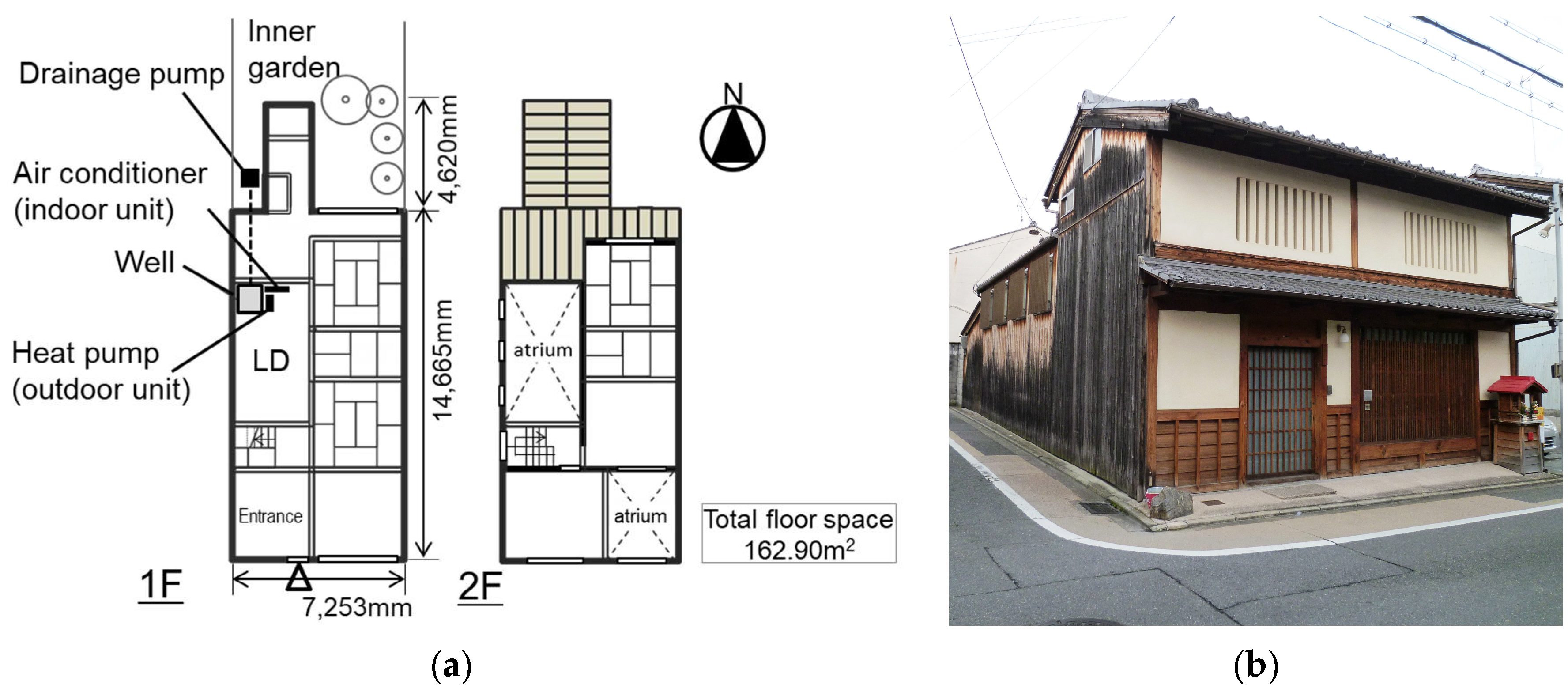
The experiment was performed in an existing Kyo-machiya dwelling, which was constructed more than 150 years ago (Figure 1). In this traditional type of dwelling, the outer and partition walls are made of soil without insulation. In this case, ceiling insulation and roof insulation was added to three rooms on the second floor in the summer of 2015. It was not even close to being airtight, however. The average U-value, which is the overall heat loss per unit of the building envelope area, of this house was estimated as 2.47 W/m2K, though the value of the energy efficiency standard was 0.87 W/m2K based on the data for moderate climate regions in Japan. The structure is rectangular, extending from south to north, and has many openings in the north and south facades, as shown in Figure 1.
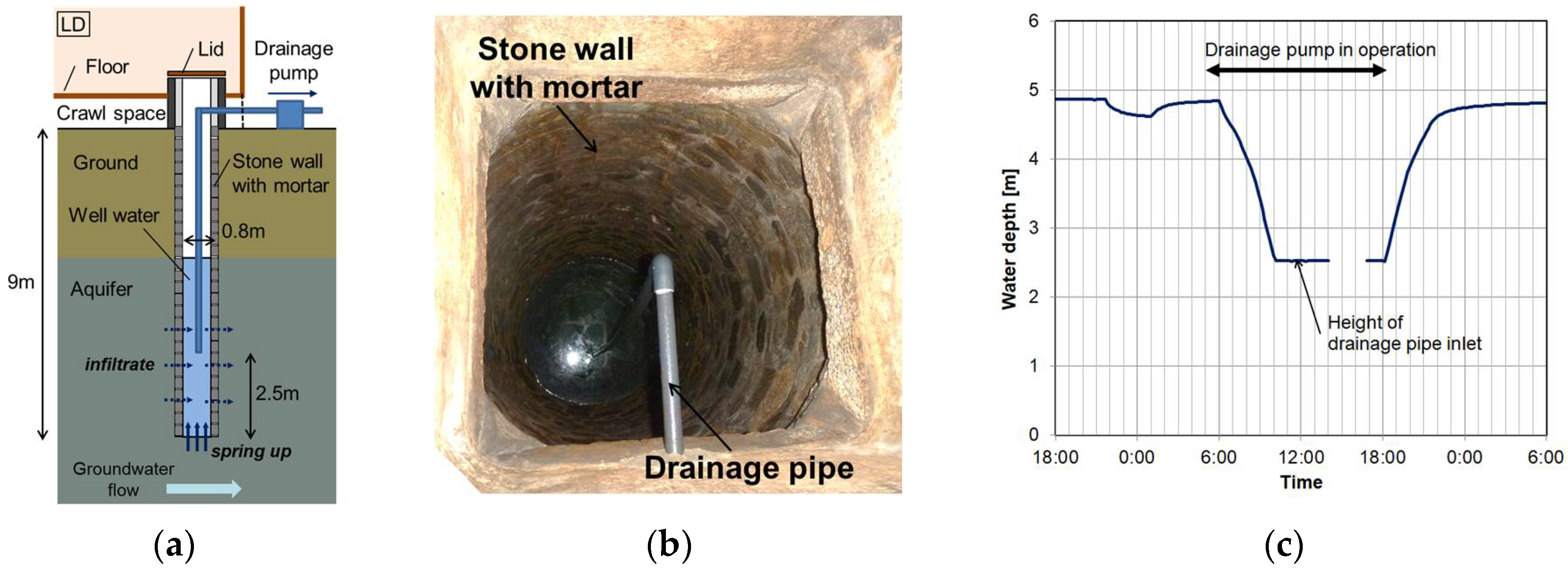
This dwelling has a well in the combined living and dining room (LD), as shown in Figure 1. The well is approximately 80 cm in diameter and reaches a depth of approximately 9 m below the ground surface, as shown in Figure 2a. This well is classified as a shallow well. The side wall of the well is made up of stones, with the gaps between the stones filled with mortar (Figure 2b). In most cases, well water springs up from the bottom of the well; however, in some cases, it infiltrates the well through the side wall. A self-priming, vortex-type drainage pump was installed in the well. It was often used to operate a sprinkler to water the plants in the courtyard and the road in front of the house. To examine the speed of drainage and the recovery of the water level, a preliminary test was conducted on 8 December 2016. Although the flowrate of the drainage pump was originally expected to be 31 L/min, the current value will be smaller due to aging degradation of the pump. The alteration in water depth is depicted in Figure 2c. The water level dropped by approximately 2.4 m in 4 h when the drainage pump was being operated. After terminating the operation, the water level was observed to recover within 5–6 h. This indicated that the flowrate of groundwater in this area was relatively high so that the water level could be recovered to the ordinary water level in the case of a shallow well. Further, it was also indicated that the inlet of the drainage pipe was installed around the middle part of the well water, as depicted in Figure 2a.
The examined heat-pump system was installed near the well in the dwelling in December 2013, and the well-water temperature and water level were continuously measured, as reported in the previous study. Table 1 shows the global performance of the heat-pump system. The rated heating capacity was 5.0 kW, suitable for a room in an 18–23 m2 wooden house (the area of the LD in this house was approximately 20 m2). As the rated heating electric power consumption was 1389 W, the rated system coefficient of performance (COP) could be calculated as approximately 3.6. A kerosene fan heater was sometimes used in the LD as an auxiliary heater.
The heat-pump system consisted of an indoor unit, an outdoor unit, a refrigerant pipe, and a heat extraction pipe passing through the water in the well. A propylene glycol diluent, used as an antifreeze solution, circulated in the heat extraction pipe. The specifications of the heat extraction pipe and antifreeze solution are shown in Table 2. The heat extracted from the water was returned to the heat pump (HP) and used as a heat source. As described above, the surveyed well was located inside the LD. Therefore, the outdoor unit, in which acoustic treatment was conducted, was also set in the LD.
In this system, the amount of blowout from the indoor unit was determined according to the difference between the set temperature and the current indoor temperature, and the refrigerant temperature circulating into the indoor unit also affects the amount. The flowrate of the antifreeze solution circulating in the well water varies depending on the indoor heat load.
When the heat-pump system was installed, the heat extraction pipe was fixed spirally, tied up using a weight, and thrown into the well. In the preliminary experiment that was mentioned above, it was also confirmed that the pipe was laid densely in the middle and lower part of the well water.
2.2. Measurement Items
The measurement items and points are shown in Figure 3. The well-water level was measured every 10 min using a pressure-type level gage, which included both ceramic pressure and temperature sensors. When calculating the water level, both the water pressure in the well and the barometric pressure that was measured in the air above the well-water surface (see Figure 3a) were used. The temperatures of the air (Ta) and the water in the well (Tw) were also obtained using the level gages. The water level logger inside the water was set so that it was 2500 mm above the bottom of the well. The same type of logger was set in the wells in three houses from the same neighborhood (NW1, NW2, and NW3) to understand the well-water situation without a heat-pump system (see Figure 3b). NW1 was expected to be located upstream of the groundwater in the surveyed well, whereas NW2 and NW3 were probably positioned downstream.
The well-water temperatures in the surveyed dwelling were measured continuously (at 1-min intervals) at distances of 500 (lower part, TL), 2500 (middle part, TM), and 4500 mm (upper part, TU) from the bottom of the well using a T-type thermocouple. After January 2018, the temperature of the area that was very close to the water surface (TS) was measured instead of that of the upper part. The flowrate of the antifreeze solution (Jb) was measured by an electromagnetic flow meter, and both the temperatures of the antifreeze solution flowing out from the heat pump (Tout) into the well and returning from the well into the heat pump (Tin) were measured using a platinum resistance thermometer sensor (Pt100).
The electric power consumption for the whole heat-pump system (Es, including for the compressor and circulation pump), and the drainage pump (Ed) were measured continuously by a clamp-type wattmeter. The drainage pump’s electric power consumption data acquisition started on 16 January 2018. The performance data of each measurement apparatus is listed in Table 3. Furthermore, we asked the residents to take note of the frequency and usage settings of both the heat-pump system and the drainage pump so that they could be acquired for data analysis.
2.3. Operation Patterns
In this experiment, the heat-pump heating system was operated as usual in this house, namely, for approximately 12 h per day from morning to evening. The different operational patterns for the drainage pump were compared. The patterns are listed in Table 4 below. A “without drainage” pattern (named “normal” operation) was conducted from December 2016 to March 2017, while a “with drainage” pattern (named “heat recovery” operation) was conducted during the latter half of January 2018. The difference in each pattern was whether the drainage pump was operated before, after, or during the heat-pump operation. Further, it was basically left to the residents to decide when to start the usage and the number of hours that they intended to use both the heat pump (HP) and the drainage pump so that the residents could feel comfortable. The representative dates that are listed in Table 4 were selected by judging whether the operation duration of the HP and the drainage pump was observed to be similar on each date. In each pattern, the drain valve was fully open because, as shown in the preliminary experiment in the first half of January, the electric power did not decrease even when the valve was tightened.
3. Results
The measurement results are shown here for two periods: December 2016–February 2017 and November 2017–January 2018.
3.1. Time Profile of Well-Water Temperature and Water Depth during Winter
The well-water temperatures, measured by water level loggers in the surveyed house and in the neighborhood wells (NW1, NW2, and NW3), are shown in Figure 4a,b, respectively. Before the heat-pump operation began, the well-water temperature in the surveyed house was about 19 °C, and this seemed to be almost the same as those in the neighboring houses. The temperature of the well water generally fluctuated from 16 °C to 20 °C in this area in the case of no usage of ground heat. When the heat pump started to operate, the well-water temperature began to decrease to around 7–8 °C (Figure 4a). In 2017–2018, as shown in Figure 4b, the heat recovery operation started after terminating the heat pump operation for a few days. The well-water temperature stayed at around 14 °C on average during the heat recovery operation.
Figure 5 shows the calculated water depth during the same period as was displayed in Figure 4. The water depth was obtained from the water level, which referred to the distance from the well-water surface to the water level logger, added to the distance from the bottom of the well. In each well, the variation in the water depth was affected by the precipitation. The water depth of the surveyed house was almost the same as that of NW2, while the depths of both NW1 and NW3 were approximately 2 m lower than that of the surveyed house. Although the water depths were different, the distances between each water level logger and the ground surface were almost the same. In this neighborhood area, the ground temperature at an identical depth was observed to be almost the same because there was plenty of horizontal groundwater flow. Therefore, the temperature in each well seemed to take a similar value. When well water was used for daily life in NW1, the depth fluctuated frequently. After the heat recovery operation was started, the depth of the surveyed house also repeatedly decreased/increased as indicated in Figure 5b.
3.2. Measurement Results in each Pattern Focusing on a Certain Day
In this section, the well-water temperature, the antifreeze solution temperature and flowrate, the electric power consumption, and the calculated system COP measurement results are shown focusing on a certain day in each pattern. The results from the normal operation without drainage are from 15 February 2017. The results from before the HP operation are from 26 January 2018. The results from during the HP operation are from 28 January 2018, and the results from after the HP operation results are from 18 January 2018.
3.2.1. Well-Water Temperature Changes at Different Heights and Water Depths
Figure 6 shows the well-water temperature at different heights and at the water level gage, as well as the water depth. The water gage was located at almost the same height as the middle part even though it seemed to be positioned closer to the center. In Figure 6a, the temperature of the well water had already been lowered due to a long period of HP operation. The temperature in the middle part was about 10 °C before the HP operation and decreased by up to 6 °C after 9 h of the HP operation. The temperature in the lower part changed almost the same way as did that of the middle part. The temperature of the upper part was over 2 °C higher than that of the middle and lower parts. Although the temperature decreased rapidly soon after the HP operation started, the temperature in the upper part was almost unchanged during the operation. As the drainage pump was not used, the water depth was kept at a fixed level.
As shown in Figure 6b–d, the temperature in the middle part was higher than that in the lower part because the heat recovery operation was done every day. When the drainage pump was used for about 1 h, the water depth decreased by 0.4 m, and the water depth recovered within 3 h. When the drainage pump was launched, the temperature in the middle part increased much more than it did in the lower part and near the water surface. During the HP operation, the temperature in the middle part increased by 2 °C, and before and after the HP operation, it increased by 3–5 °C, depending on the temperature before the operation. As the well-water temperature was low at the end of the HP operation and temperature difference between the well water and the peripheral ground was greater at that time, the degree of temperature recovery was the greatest in the case where the drainage pump was launched after the HP operation.
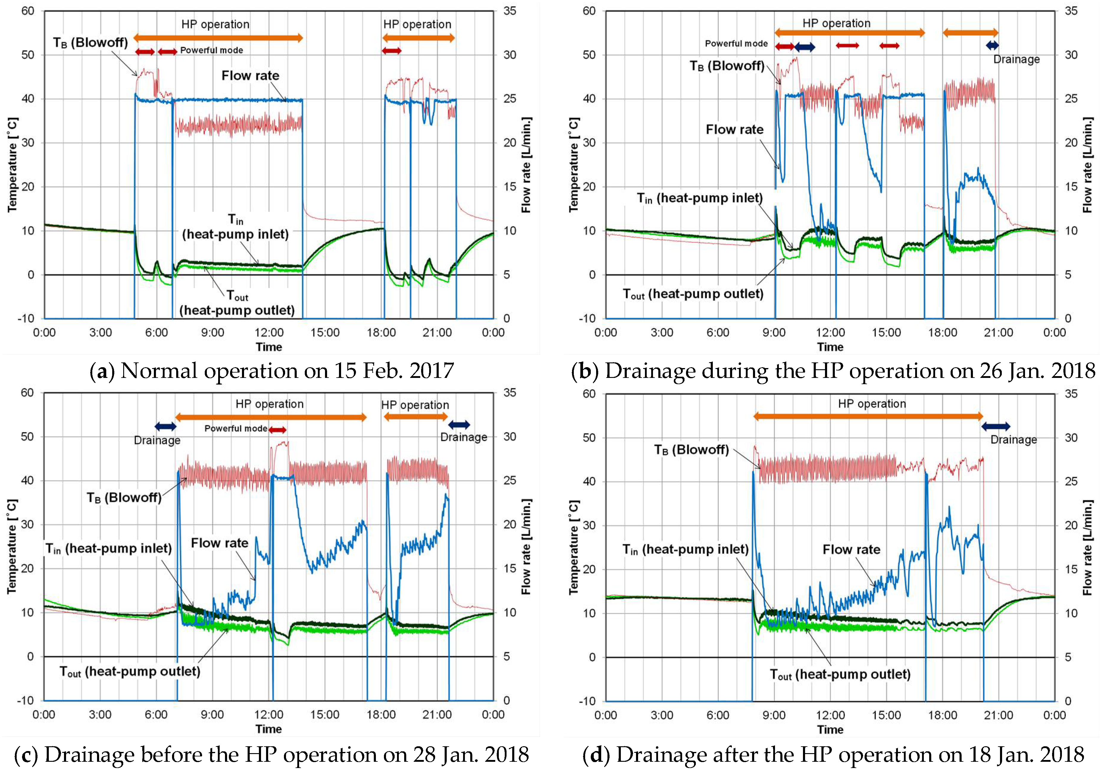
3.2.2. Temperature and Flowrate of Antifreeze Solution and Heating Blowoff Temperature
The antifreeze solution temperature measured at the inlet and outlet of the heat pump and the flowrate are shown in Figure 7 along with the heating blowoff temperature. The antifreeze solution (with its initial temperature) circulated in the well water and returned with an increased temperature. When the HP was launched or the heat load was higher, the HP worked in “powerful mode”. In this mode, the heating blowoff temperature was kept high—at around 45–50 °C. To attain the high blowoff temperature, the antifreeze solution temperature must be kept at a lower temperature. The amount of heat gain was calculated by the flowrate and antifreeze solution temperature difference between the inlet and outlet of the heat pump. As the antifreeze solution temperature decreased, the temperature difference also decreased, and the flowrate increased automatically to maintain the necessary heat gain. Therefore, the flowrate in the normal operation (Figure 7a) was kept at a maximum value of 25 L/min.
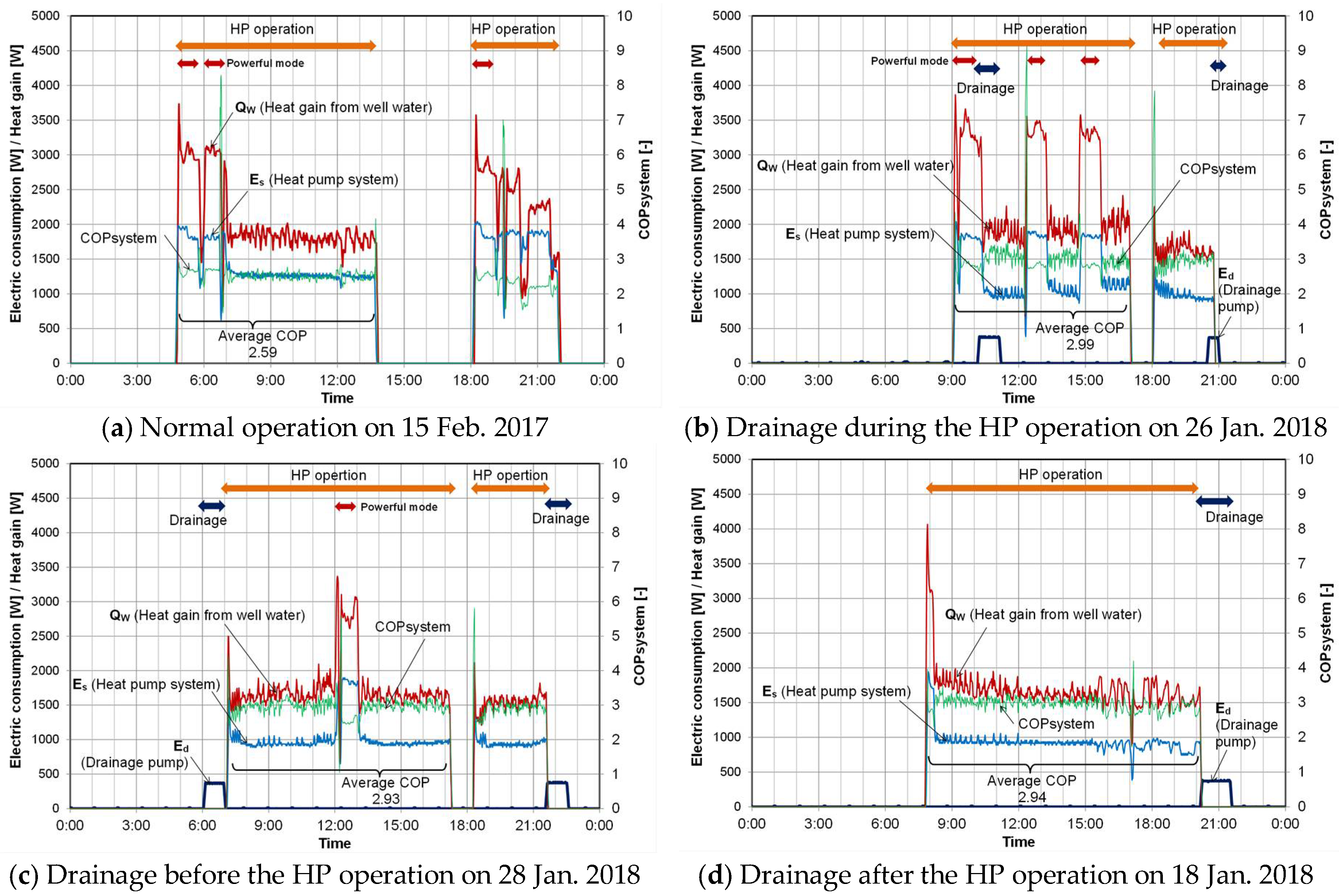
3.2.3. Electric Power Consumption of the HP System and the Drainage Pump and Coefficient of Performance
Using the measured temperatures and flowrate of the antifreeze solution, the heat gain from the well Qw (W) can be calculated by the following equation:
where Tin and Tout are the temperatures (K) of the antifreeze solution at the heat-pump inlet and outlet, respectively. The density and specific heat of the propylene glycol diluent are both assumed to be constant, where cb = 4.1 × 10³ (J/kg·K) and ρb = 1.02 × 10³ (kg/m3). Jb is the flowrate of the antifreeze solution (m3/s). Where the power consumptions of the heat pump (compressor and auxiliary equipment) and the antifreeze solution circulation pump are Eh and Ep, respectively, the power consumption in the entire heat-pump system ES is expressed as (Eh + Ep). Then, the amount of heat Qh supplied as heating energy to the indoor space is expressed by the sum of the heat gain Qw and power consumption ES. The COP of the overall HP system was calculated by Equation (2) below:
Figure 8 depicts the electric power consumption of the HP system and the drainage pump, the calculated heat gain from the well Qw, and the calculated COPsystem. These data were shown as moving averages for successive 5-min intervals. During normal operation, where the well water was kept at a lower level, the average COP from 5:00 to 14:00 on 15 February 2017 was 2.59. The average COP in each heat recovery operation was also presented in Figure 8. The average COP for three days of heat recovery operation was 2.95. Thus, the efficiency increased by approximately 14%.
4. Discussion
4.1. Well-Water Increase Caused by Operating Drainage Pump
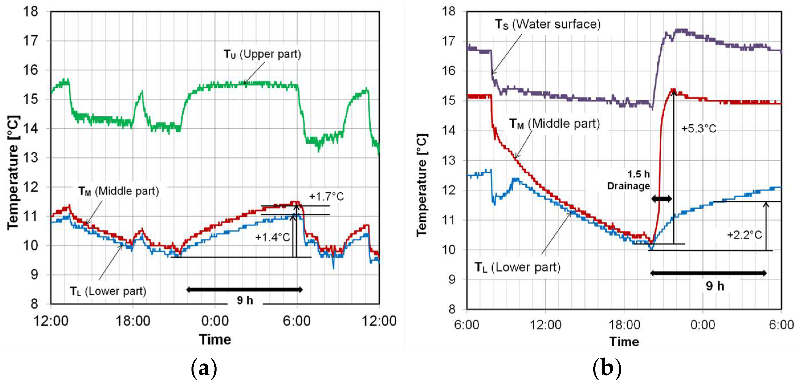
Figure 9 shows the typical temperature change with and without operating the drainage pump after using the HP system. If the drainage pump was not used, the temperatures in the middle and lower parts changed in the same way and increased by 1.7 °C and 1.4 °C within 9 h, respectively. On the other hand, as described in Section 3, the temperature in the middle part rapidly increased when the drainage pump was launched; the temperature increased by 5.3 °C in only 1.5 h. The temperature in the lower part also increased by 2.2 °C within 9 h.
There are two possible reasons for this, considering that the drainage pipe inlet in the well water was located near the temperature measurement point in the middle part. One reason is that the warmer underground water can infiltrate through the well wall around the middle part. Although the well wall was made of stones and mortar, many cracks seemed to exist in the mortar part. Actually, it was observed that the groundwater infiltrated through the sidewall once the well water was drained as much as possible. The second reason is that the warmer water in the upper part could have sunk down toward the middle part. However, as the temperature near the water surface also increased, it cannot be explained by only this reason. It can be estimated that the water infiltration has a greater influence on temperature recovery. Thus, the water path into the well should be examined in detail.
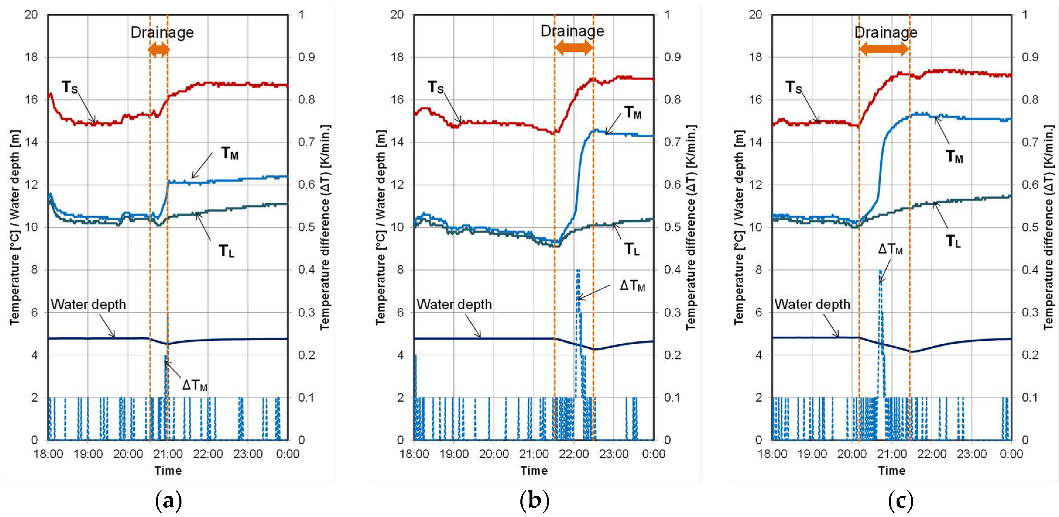
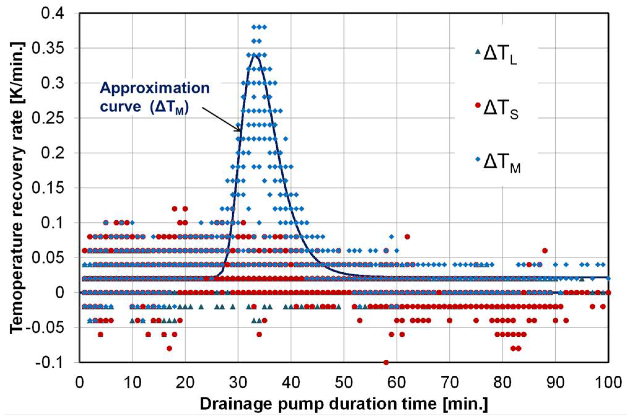
Based on the measured water depth, it is possible to conclude that plenty of groundwater flows underground in this area. The temperature recovery rate was examined in terms of the drain pump duration. Figure 10 shows the relation between the drainage duration and the temperature recovery rate in the middle part along with the well-water temperatures. Here, the temperature recovery rate indicates the temperature difference per minute. The temperature recovery rates in each part of the well during the drainage pump operation from 17 January 2018 to 31 January 2018 are depicted in Figure 11. In this case, the temperature recovery rate reached its peak after approximately 33 min in the middle part; although, a distinct peak could not be observed in the upper and lower parts. The temperature of the well water in the middle part continued to gently increase, even after 30 min, until a period of 1 h. It can be observed that operating the drainage pump for 30 min is not sufficient to recover the temperature; however, a longer operation of more than 1 h will result in an additional increase in electric power consumption.
4.2. Improvement of Heat Gain and Energy Efficiency
In this heat-pump heating system, the flowrate of the antifreeze solution was automatically controlled depending on the temperature difference of the antifreeze solution at the heat-pump inlet and outlet to ensure that the target heat gain was achieved. The higher well-water temperature helped the antifreeze solution temperature difference to increase, and it reduced the circulation pump’s electric power consumption. Another added bonus was that the sound of the circulation pump became lower. Acoustic problems cannot be ignored in individual houses. Furthermore, the temperature of the antifreeze solution does not have to be excessively lowered when the well-water temperature is higher. This can save the compressor’s electric power usage. While the drainage can cause well-water temperature recovery, it uses extra electric power for the drainage pump. Table 5 shows the effect of the COP improvement in comparison with the extra energy consumption in this case. The energy saving effect, ΔE, which is defined as the energy consumption difference between the increase by the drainage pump and the decrease by the COP improvement, was calculated using the following equation:
The definitions of the symbols that appear in Equation (3) are presented in Table 5. When the heat-pump system is used for 8–12 h in a day and the drainage pump is used for 1 h, the total electric power consumption can be lowered by 1.3–1.4 kWh per day. Considering that the drainage pump is also used for daily activities, such as watering the plants, the power consumption is not necessarily an extra increase. It should be operated appropriately for both purposes.
5. Conclusions
In this study, a highly effective usage of the ground-source heat-pump system in the case of an existing well at a traditional dwelling in Kyoto was investigated; the well was verified to possess sufficient heating capacity with the help of a previous study. If a heat-pump system is continuously used, the well-water temperature will continue to decrease and the heat extraction efficiency will become lower. Therefore, a heat recovery experiment was conducted to examine the improvement in the heat recovery performance by forced drainage of the well water. The experimental results revealed that maintaining a relatively high temperature of the well water, along with suitable amounts of drainage, helped to maintain a higher COP. In this case, the temperature recovery rate of the middle part in the well was observed to exhibit a distinct peak at around 33 min after initiating the drainage pump operation; thus, it may not be necessary to use the drainage pump for so long. The energy-saving effect of improving the COP may exceed the drawback of the increase in electric power consumption produced by the short-time drainage pump operation. Furthermore, it is recommended that the drainage pump be initiated after completing the HP operation, at which time the temperature of the well water is the lowest. The greater the temperature difference between the well water and the infiltrating groundwater, the more efficient the manner in which the temperature can be recovered.
Because the potential amount and flowrate of groundwater very depending on the location, a preliminary experiment related to drainage and water-level recovery is essential. If the position of the groundwater inflow to the well has been specified, we suggest that the heat extraction pipe be installed densely near that position. The method proposed in this study can be helpful for designing a simple ground-source heat-pump system in dwellings or small buildings.
Author Contributions
Chiemi Iba conceived of and designed the experiments and wrote the paper. Shun Takano performed the experiments and analyzed the data. Shuichi Hokoi contributed to the experimental design and gave important suggestion about the entire content.
Acknowledgments
This study was partially supported by LIXIL JS Foundation, Research Grants 2013. The authors extend sincere gratitude to Yoshihide Tamura and Mariko Takeda for their kind help in conducting the experiment. Additionally, the authors would like to thank Enago (www.enago.jp) for the English language review.
Conflicts of Interest
The authors declare no conflict of interest.
References
- Sanner, B.; Nordell, B. Underground thermal energy storage with heat pumps—An International Overview. IEA Heat Pump Centre Newslett. 1998, 16, 10–14. [Google Scholar]
- Sanner, B.; Karytsas, C.; Mendrinos, D.; Rybach, L. Current status of ground source heat pumps and underground thermal energy storage in Europe. Geothermics 2003, 32, 579–588. [Google Scholar] [CrossRef]
- Hamada, Y.; Nakamura, M.; Ochifuji, K.; Nagano, K.; Yokoyama, S. Field performance of a Japanese low energy home relying on renewable energy. Energy Build. 2001, 33, 805–814. [Google Scholar] [CrossRef]
- Nagano, K.; Katsura, T.; Takeda, S. Development of a design and performance prediction tool for the ground source heat pump system. Appl. Therm. Eng. 2006, 26, 1578–1592. [Google Scholar] [CrossRef]
- Tarnawski, V.R.; Leong, W.H.; Momose, T.; Hamada, Y. Analysis of ground source heat pumps with horizontal ground heat exchangers for northern Japan. Renew. Energy 2009, 34, 127–134. [Google Scholar] [CrossRef]
- Congedo, G.S.P.M.; Colangelo, G. Horizontal Heat Exchangers for GSHPs. Efficiency and Cost Investigation for Three Different Applications. In Proceedings of the ECOS 2005 the 18th International Conference on Efficiency, Cost, Optimization, Simulation, and Environmental Impact of Energy Systems, Trondheim, Norway, 20–22 June 2005. [Google Scholar]
- Congedo, P.M.; Colangelo, G.; Starace, G. CFD simulations of horizontal ground heat exchangers: A comparison among different configurations. Appl. Therm. Eng. 2012, 33–34, 24–32. [Google Scholar] [CrossRef]
- D’Arpa, S.; Colangelo, G.; Starace, G.; Petrosillo, I.; Bruno, D.E.; Uricchio, V.; Zurlini, G. Heating requirements in greenhouses farming in southern Italy: Evaluation of ground-source heat pump utilization compared to traditional heating systems. Energy Effic. 2016, 9, 1065–1085. [Google Scholar] [CrossRef]
- Hagihara, K.; Iba, C.; Hokoi, S. Effective use of a ground-source heat-pump system in traditional Japanese “Kyo-machiya” residences during winter. Energy Build. 2016, 128, 262–269. [Google Scholar] [CrossRef]
- Fukumiya, K.; Hirao, N. Performance Characteristics of Geothermal Heat Pump System by Using an Old Well. J. Jpn. Soc. Agric. Mach. 2012, 74, 4–8. (In Japanese) [Google Scholar]
- Wang, Y.; Liu, K.W.Q.; Jin, Y.; Tu, J. Improvement of energy efficiency for an open-loop surface water source heat pump system via optimal design of water-intake. Energy Build. 2012, 51, 93–100. [Google Scholar] [CrossRef]
- Alberti, L.; Antelmi, M.; Angelotti, A.; Formentin, G. Geothermal heat pumps for sustainable farm climatization and field irrigation. Agric. Water Manag. 2018, 195, 187–200. [Google Scholar] [CrossRef]
Figure 1.
Surveyed Kyo-machiya home: (a) floor plan and (b) exterior image.

Figure 2.
Information of the well: (a) schematic cross-section; (b) images of the well; and (c) change in the depth of water during the drainage-pump operation.
Figure 2.
Information of the well: (a) schematic cross-section; (b) images of the well; and (c) change in the depth of water during the drainage-pump operation.

Figure 3.
Measurement points. (a) Schematic of the measuring points and equipment. (b) Location of neighborhood wells (NWs). TS: well-water temperature close to the water surface; TL: well-water temperature in the lower part (distances of 500); TM: well-water temperature in the middle part (distance of 2500); and TU: well-temperature in the upper part (distance of 4500 mm).
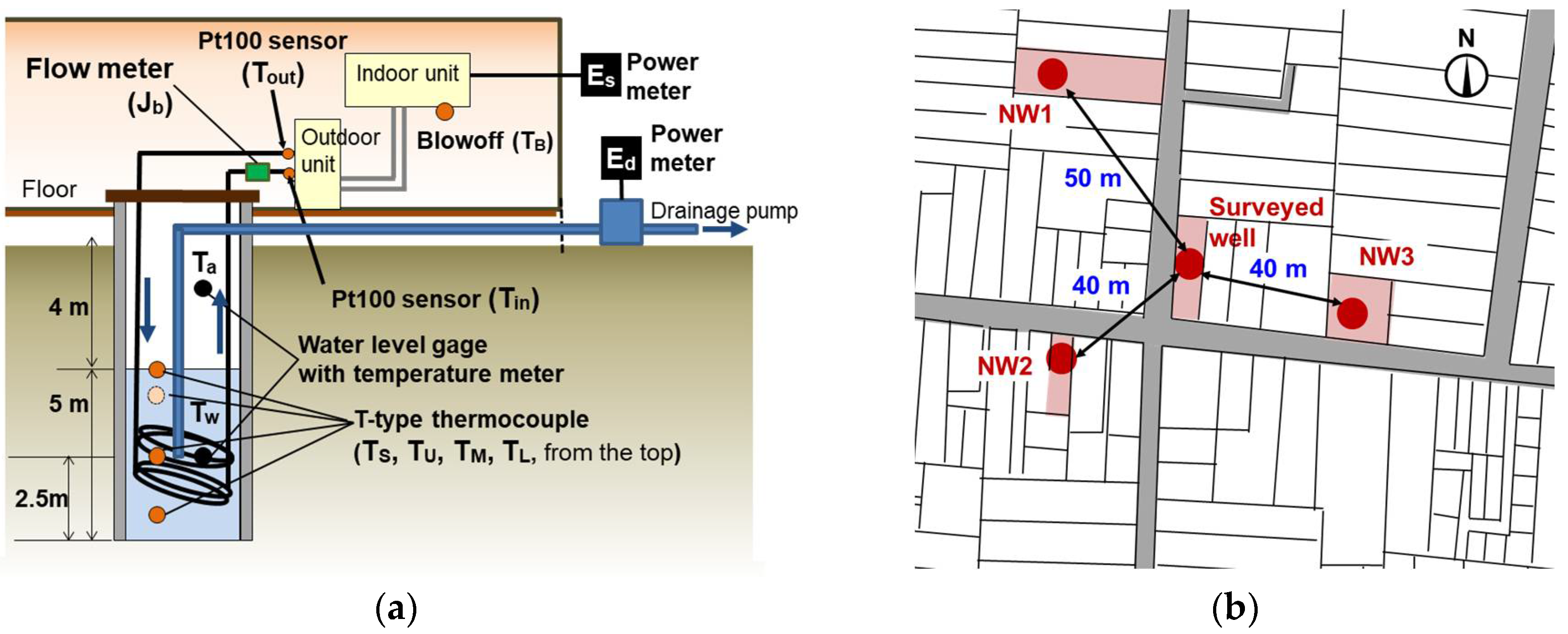
Figure 4.
Well-water temperature changes along with the neighborhood well-water temperatures.
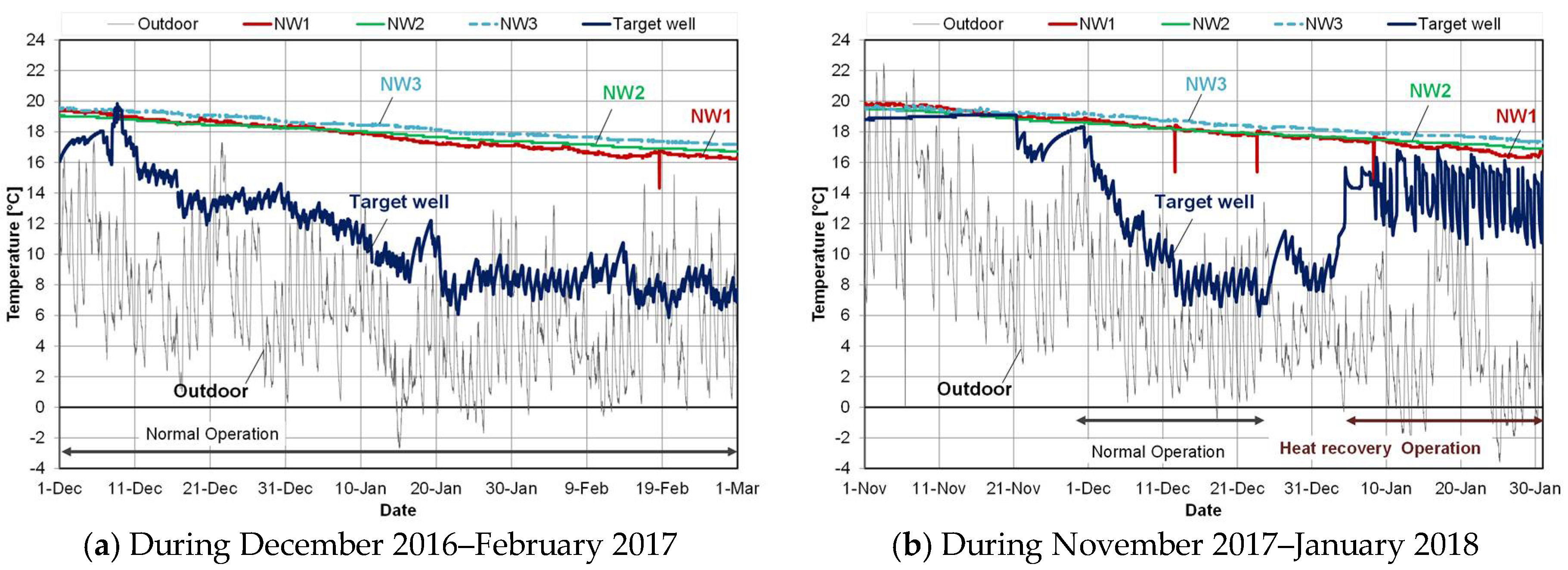
Figure 5.
Well-water depth changes along with the neighborhood well.
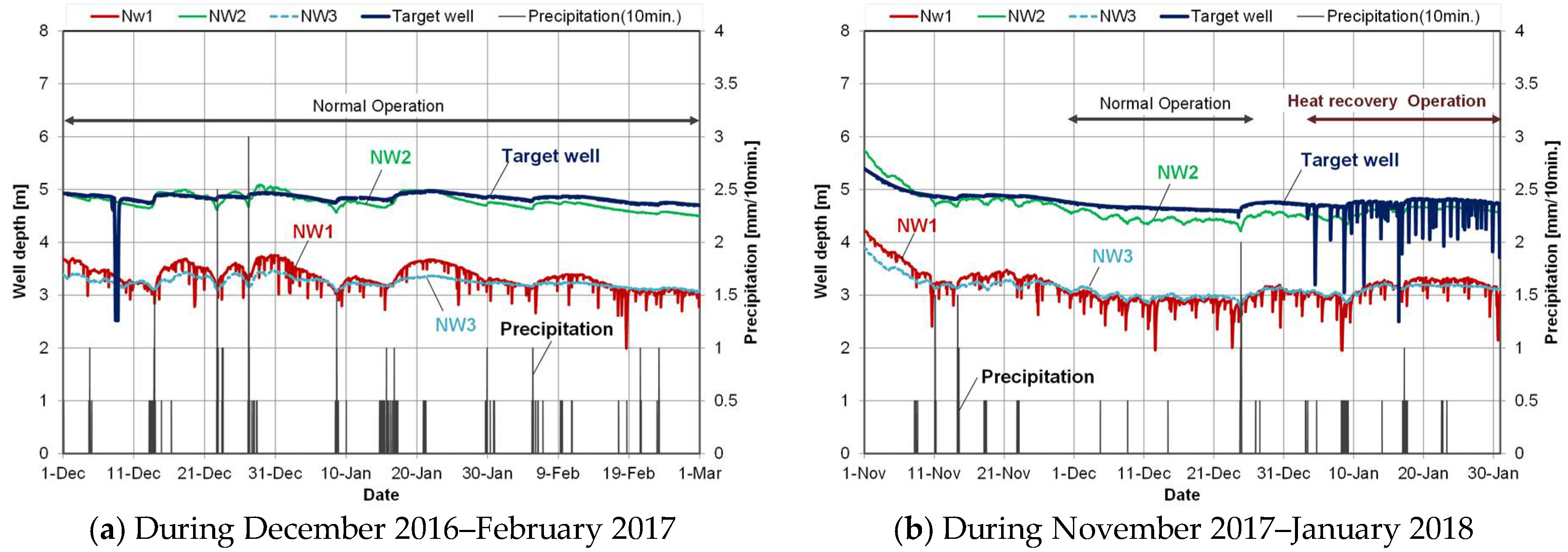
Figure 6.
Well-water temperature and water depth changes in each operation pattern.
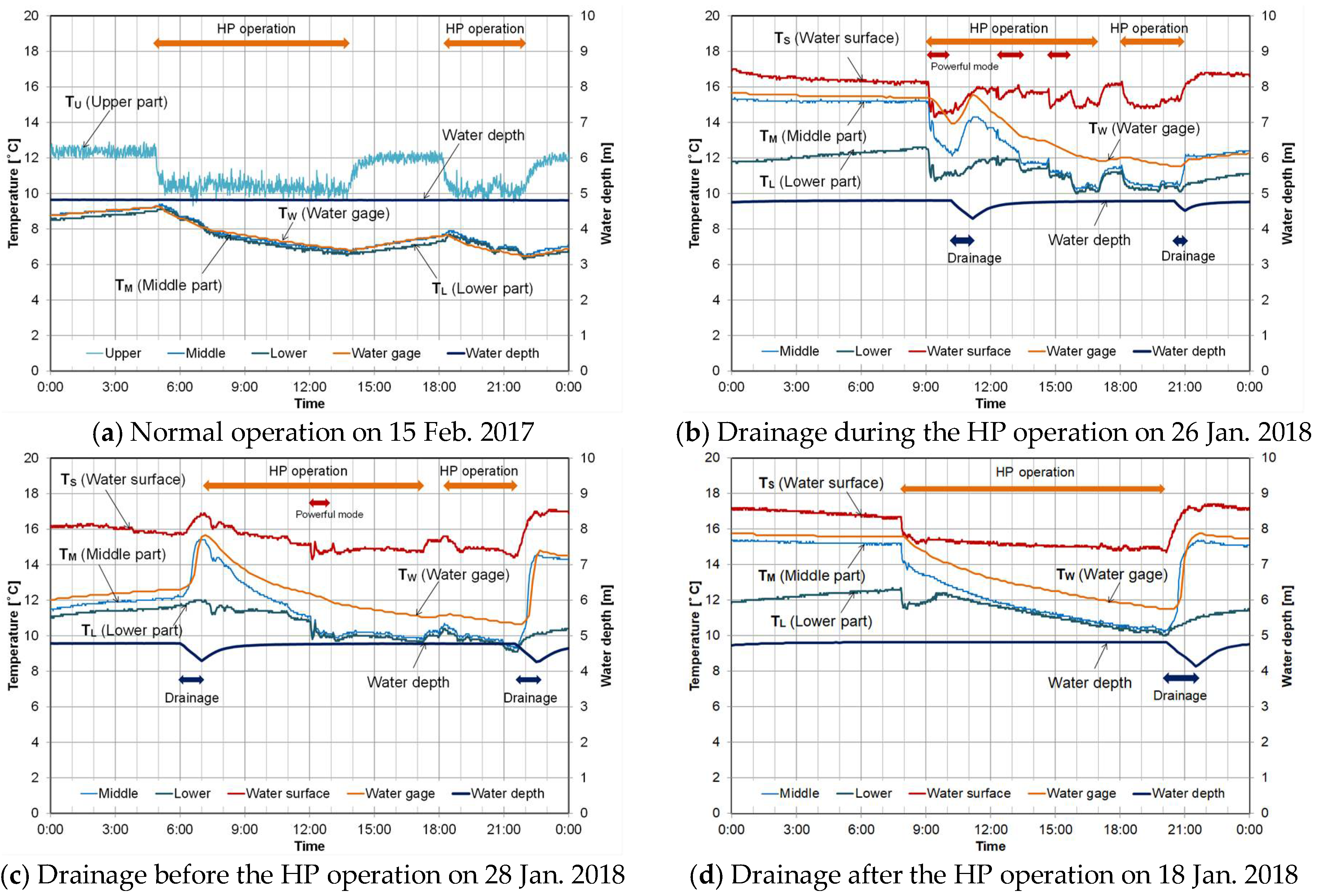
Figure 7.
Antifreeze solution temperature and flowrate change in each operation pattern.

Figure 8.
Electric power consumption and efficiency change in each operation pattern.

Figure 9.
Comparison of temperature recovery with and without drainage: (a) no drainage pump operation and (b) drainage pump operation after using the heat pump.
Figure 9.
Comparison of temperature recovery with and without drainage: (a) no drainage pump operation and (b) drainage pump operation after using the heat pump.

Figure 10.
Well-water temperature change and the temperature recovery rate in different drainage durations: (a) 0.5 h, (b) 1 h, and (c) 1.5 h.
Figure 10.
Well-water temperature change and the temperature recovery rate in different drainage durations: (a) 0.5 h, (b) 1 h, and (c) 1.5 h.

Figure 11.
Change in the temperature recovery rate during the drainage pump operation.


Table 1.
Global performance of heat-pump system.
| Type/Use | Split type (Indoor Unit/Outdoor Unit) Heating and Cooling | |
|---|---|---|
| Rated Value for the System | Heating capacity | 5.0 kW |
| Heating electric power consumption | 1389 W | |
| Heating COP | 3.60 * | |
| Compressor type/Refrigerant type | Rotary compressor/R410A | |
| Rated Value for the Compressor | Rated electric power | 1239 W |
| Heating COP | 4.04 (Evaporation Temp: 7~8 °C; Condensation Temp: 49~50 °C) | |
* When the temperature of return flow to the ground is 5 °C. COP: coefficient of performance.
Table 2.
Specifications of heat extraction pipe and antifreeze solution.
| Heat Extraction Pipe | Antifreeze Solution | ||
|---|---|---|---|
| Material designation | PE100; Allowable maximum pressure 1.60 MPa @20 °C | Material | propylene glycol 30% diluent |
| Size | Outer diameter 32 mm, pipe thickness 3 mm, 26.0 m length (16.0 m spirally set in the well water) | Density | 1020 (kg/m3) |
| Pipe thermal conductivity | 0.46–0.50 (W/mK) | Specific heat | 4010 (J/kg·K) |
Table 3.
Performance of the measurement apparatuses.
| Apparatus | Range | Accuracy | Resolution | Note |
|---|---|---|---|---|
| Pressure-type level gage | 0–4 m | ±0.3 cm | 0.14 cm | in water level |
| −20 °C to +50 °C | ±0.44°C from 0 °C to 50 °C | 0.1°C @ 20 °C | in temperature | |
| T-type thermocouple | −200 °C to +300 °C | ±0.5 °C | - | - |
| Pt100 sensor | −200 °C to +100 °C | ±(0.30 + 0.005t) °C | - | B-class |
| clamp-type wattmeter | 0–10 kW | ±3% | 0.1 W | - |
Table 4.
Operation pattern.
| Pattern | Drainage Pump | Representative Date | HP Operation Duration | Drainage Pump Duration * |
|---|---|---|---|---|
| Normal | No operation | 15 February 2017 | 9 h | - |
| Heat recovery | During the HP operation | 26 January 2018 | 8 h | 1 h |
| Before the HP operation | 28 January 2018 | 10 h | 1 h | |
| After the HP operation | 18 January 2018 | 12 h | 1.5 h |
* The flowrate of the drainage pump was expected to be 31 [L/min]. HP: heat pump.
Table 5.
Effect of the COP improvement vs the extra electric power consumption for the drainage pump.
Table 5.
Effect of the COP improvement vs the extra electric power consumption for the drainage pump.
| Pattern | Drainage Pump | Average COP (COPex) | Cumulative HP Energy Consumption (kWh) (Eex) | HP Energy Consumption * (kWh) Assumed at COPim = 2.59 | Drainage Pump Energy Consumption (kWh) (EDP) | Energy Saving Effect (kWh) (ΔE) |
|---|---|---|---|---|---|---|
| Normal | No operation | 2.59 | 12.35 at 9 h | 12.35 | 0 | 0 |
| Heat recovery | During the HP operation | 2.99 | 10.69 at 8 h | 12.34 | 0.365 at 1 h | −1.29 |
| Before the HP operation | 2.93 | 10.50 at 10 h | 11.88 | 0.339 at 1 h | −1.40 | |
| After the HP operation | 2.94 | 11.50 at 12 h | 13.05 | 0.501 at 1.5 h | −1.05 |
* Assumed that same heating applied to the room as the actual situation.
© 2018 by the authors. Licensee MDPI, Basel, Switzerland. This article is an open access article distributed under the terms and conditions of the Creative Commons Attribution (CC BY) license (http://creativecommons.org/licenses/by/4.0/).
Share and Cite
MDPI and ACS Style
Iba, C.; Takano, S.; Hokoi, S. An Experiment on Heat Recovery Performance Improvements in Well-Water Heat-Pump Systems for a Traditional Japanese House. Energies 2018, 11, 1023. https://doi.org/10.3390/en11051023
AMA Style
Iba C, Takano S, Hokoi S. An Experiment on Heat Recovery Performance Improvements in Well-Water Heat-Pump Systems for a Traditional Japanese House. Energies. 2018; 11(5):1023. https://doi.org/10.3390/en11051023
Chicago/Turabian StyleIba, Chiemi, Shun Takano, and Shuichi Hokoi. 2018. "An Experiment on Heat Recovery Performance Improvements in Well-Water Heat-Pump Systems for a Traditional Japanese House" Energies 11, no. 5: 1023. https://doi.org/10.3390/en11051023
Note that from the first issue of 2016, this journal uses article numbers instead of page numbers. See further details here.