Article

A Novel Intelligent Method for the State of Charge Estimation of Lithium-Ion Batteries Using a Discrete Wavelet Transform-Based Wavelet Neural Network

1
Graduate School at Shenzhen, Tsinghua University, Shenzhen 518055, China
2
Sunwoda Electronic Co. Ltd., Shenzhen 518108, China
*
Author to whom correspondence should be addressed.
Energies 2018, 11(4), 995; https://doi.org/10.3390/en11040995
Submission received: 2 April 2018 / Revised: 13 April 2018 / Accepted: 16 April 2018 / Published: 20 April 2018

Abstract

:
State of charge (SOC) estimation is becoming increasingly important, along with electric vehicle (EV) rapid development, while SOC is one of the most significant parameters for the battery management system, indicating remaining energy and ensuring the safety and reliability of EV. In this paper, a hybrid wavelet neural network (WNN) model combining the discrete wavelet transform (DWT) method and adaptive WNN is proposed to estimate the SOC of lithium-ion batteries. The WNN model is trained by Levenberg-Marquardt (L-M) algorithm, whose inputs are processed by discrete wavelet decomposition and reconstitution. Compared with back-propagation neural network (BPNN), L-M based BPNN (LMBPNN), L-M based WNN (LMWNN), DWT with L-M based BPNN (DWTLMBPNN) and extend Kalman filter (EKF), the proposed intelligent SOC estimation method is validated and proved to be effective. Under the New European Driving Cycle (NEDC), the mean absolute error and maximum error can be reduced to 0.59% and 3.13%, respectively. The characteristics of high accuracy and strong robustness of the proposed method are verified by comparison study and robustness evaluation results (e.g., measurement noise test and untrained driving cycle test).

1. Introduction

The battery management system (BMS) is responsible for monitoring power batteries’ complete information to guarantee the electric vehicle (EV) performance, because the batteries’ parameters such as current, voltage, resistance, and temperature are of importance, indicating the safety and normality of the power system [1]. State of Charge (SOC) has an undoubted critical position for BMS to realize management functions, and it indicates the remaining energy, whose accuracy is of great significance for service safety and life of batteries [2,3]. Nevertheless, the limitation on the progress of BMS is mostly due to SOC unmeasurable and dynamic properties that are similar to the characteristics of the batteries, which are influenced by various factors [4], such as discharge rate, ambient temperature, battery degeneration, and external disturbance. Therefore, the study of high accuracy SOC estimation methods is vitally important using measureable variables, such as current, voltage and temperature.
With the rapid development of EV and the increasing importance of BMS, numbers of estimation approaches have been proposed to monitor the SOC. The ampere-hour (A·h) integral or Coulomb counting method [5,6] and open-circuit voltage method [7] are simple to implement, but non-model based and open-loop characteristics limit their precision on account of the inaccurate initial SOC measurement noise and ambient disturbance [8].
Model-based methods are the hot area of recent research, such as the Kalman filter (KF)-class methods (e.g., the extended Kalman filter (EKF) [9,10,11,12], cubature Kalman filter (CKF), and unscented Kalman filter (UKF) [13,14]), observer based methods (e.g., sliding mode observer (SMO) [15,16], Luenberger observer [17,18], and multi-time-scale observer [19]) and particle filter (PF) [20,21]. Based on the proposed battery models (e.g., the well-used equivalent circuit model [22,23], the relative more complex electrochemical model [17,18,24], and the electrical thermal model [11]), model-based methods have satisfying results in SOC estimation in terms of high accuracy level and robustness against measurement error, especially the online, model-based SOC estimation methods [12,25]. Nevertheless, there are shortcomings in the application of model-based methods. For instance, the EKF method is influenced by the initial parameters and has to face large linearization errors [16]. Furthermore, the assumption that the noise is approximate to Gaussian white noise and the statistic property of measurement noises is known should be satisfied, which is the basement for KF-class methods. The PF method has the requirement for numbers of particles and matrix operations causing limitations to its application. As for SMO method, it is hard to obtain the optimal parameters that leads to the process of SOC estimation complex. Undoubtedly, model-based methods have performed excellently in current research, but model parameters identification using various optimization methods is costly and time-consuming. For instance, the second-order equivalent circuit model-based KF-class methods to estimate SOC should not only identify the resistors and capacitors value but also ascertain the temperature related relationship between open-circuit voltage (OCV) and SOC. The charging process is supposedly equally important for batteries that has been studied valuably as well [26]. Therefore, in the application process, more experiments, such as the hybrid power pulse characteristics (HPPC) experiment and the experiment to ascertain OCV-SOC relationship, have to be conducted, which are complex and costly.
Artificial neural networks (ANNs) methods are not based on the detailed knowledge of the battery model (e.g., the back-propagation neural network (BPNN) [27,28], support vector machine (SVM) network, radial neural network (RNN) [29,30], and wavelet neural network (WNN) [31,32]). For ANNs, the SOC estimation problem can be regarded as a nonlinear system identification problem, and a trained ANN can be described as the model of identified batteries. Therefore, to some extent, ANN-based SOC estimation methods can avoid the problems of non-model-based methods and can be more practical than physical model-based methods. Furthermore, along with the fast development of artificial intelligence and the rapid progress of the driverless car, deeper research on ANN-based SOC estimation methods is required to correspond to technological development. Nevertheless, ANN methods have drawbacks as well. The accuracy of training data directly influences the model approximation effect, and more neurons are needed to increase the approximation ability of complex system [33]. The large training time of the ANNs-based method is also an unavoidable problem. WNN is one important branch of ANNs because of its considerable nonlinear function approximation ability and great robustness, which are in terms of the combination of the wavelet decomposition property and self-learning ability [34]. The wavelet decomposition process can considerably reduce the influence of errors, and the mathematics foundation of WNN can minimize the needed number of neurons.
WNNs can be classified according to the combining method of wavelet decomposition and ANNs. The hybrid WNN is well studied, which simply connects the computation process of the discrete wavelet multi-resolution decomposition with the multi-layer perceptron [35,36,37]. Another kind of WNN is the multi-resolution analysis (MRA) structure-based neural network, which is a kind of more tightly bound WNN, but the structure and learning process are limited by MRA theory, which is not flexible to confirm [38]. Adaptive WNN is developed based on the BPNN, which replaces the excitation function with wavelet functions [39]. The auto-generating parameters of adaptive WNN make the neural network model easy to establish and apply to the estimation method. Little research studies the combination of the hybrid WNN connecting method and the adaptive WNN.
The field of WNN-based SOC estimation needs more study. Most researches mainly focus on the denoising ability of discrete wavelet transform (DWT) [40,41,42]. The hybrid WNN [43] -based SOC estimation methods; adaptive WNN-based [32] in 2005; and momentum-optimized, adaptive WNN [31]-based in 2013 SOC estimation methods are discussed, which have good performance facing the high nonlinear battery system, but the training algorithm is based on the steepest descent method, and the study of the hybrid WNN using the wavelet multi-resolution decomposition method to optimized the adaptive WNN is quite limited. The combination is supposed to have high accuracy estimation ability on SOC.
To solve the above problems, this paper combines the adaptive WNN with the hybrid WNN and proposes a kind of novel, intelligent SOC estimation method that is expressed as the DWT and Levenberg-Marquardt (L-M) algorithm-based WNN (DWTLMWNN). The adaptive WNN is trained by L-M algorithm and, importantly, the input signals are from the data processed by discrete wavelet decomposition and reconstitution. The SOC, in discharge process under the New European Driving Cycle (NEDC), is estimated by BPNN, EKF, and the proposed WNN-based methods as a comparison. Estimation robustness is discussed by the untrained driving cycle test and measurement noise test.
The remaining part of this paper is organized as follows. Section 2 introduces the adaptive WNN model. The L-M algorithm and DWT optimizing process are presented in Section 3. The experimental validation of the proposed method and discussion are proposed in the Section 4. In the end, the paper is summarized in Section 5.

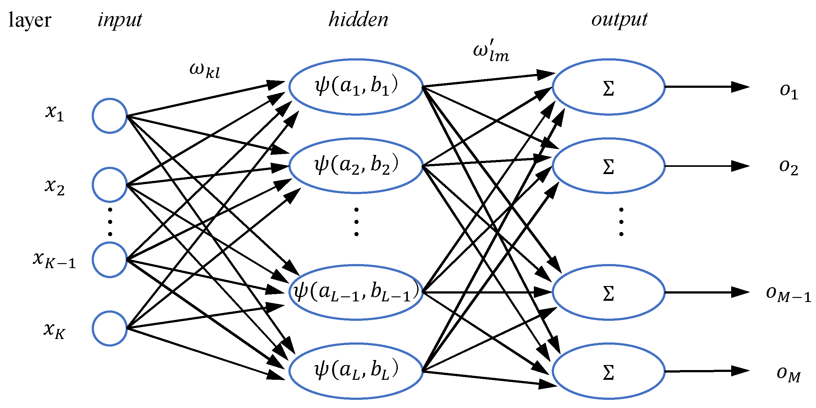
2. Estimation Model Based on WNN

The definition of SOC is commonly defined as the ratio of the remaining capacity to the nominal capacity and formulated as
S O C ( t ) = S O C ( t 0 ) 1 C n t 0 t i ( τ ) d τ
in which i ( τ ) and C n , respectively, denote the battery current and the nominal capacity of the battery.
The adaptive WNN has good performance for the reason that the parameters of wavelet templates can be adaptively generated[39]. As shown in Figure 1, there are three layers (input layer, hidden layer, and output layer) that consist of K, L, and M nodes, respectively. The input data and output data are presented by x k and o m . The weights ω k l and ω l m ' , the wavelet translation parameter b l , and wavelet dilation parameter a l are the main parameters adjusted corresponding to the learning process. x l ' is defined as the output of the hidden layer, which is formulated as
x l ' = ψ a l , b l ( n e t l ) ( l = 1 , 2 , ... , L )
n e t l = k = 1 K ω k l x k b l a l ( l = 1 , 2 , ... , L )
in which ψ ( x ) denotes the generating functions, and in this paper ψ ( x ) is defined as Morlet wavelet function:
ψ ( x ) = cos ( 1.75 x ) exp ( 0.5 x 2 )
The outputs of output layer’s nodes are formulated as
x m ' ' = n e t m ' = l = 1 L ω l m ' x l ' ( m = 1 , 2 , ... , M )
Firstly, the process of training WNN is demonstrated basing the steepest descent algorithm as a basis of following section. The output mean square error is defined as
E = 1 2 m = 1 M ( x m ' ' o m ) 2
The weights and wavelet parameters can be adjusted as follows:
ω k l * = ω k l + Δ ω k l
ω l m ' * = ω l m ' + Δ ω l m '
a l * = a l + Δ a l
b l * = b l + Δ b l
in which Δ ω k l , Δ ω l m ' , Δ a l , and Δ b l are calculated as
Δ ω k l = η E ω k l = η E n e t l n e t l ω k l = η E x l ' x l ' n e t l n e t l ω k l
Δ ω l m ' = η E ω l m ' = η E n e t m ' n e t m ' ω l m '
Δ a l = η E a l = η E n e t l n e t l a l = η E x l ' x l ' n e t l n e t l a l
Δ b l = η E b l = η E n e t l n e t l b l = η E x l ' x l ' n e t l n e t l b l
in which we have
E x l ' = m = 1 M ( x m ' ' o m ) ω l m '
x l ' n e t l = ψ ( 1 ) ( n e t l )
n e t l ω k l = x k a l
n e t l a l = k = 1 K ω k l x k b l a l 2
n e t l b l = 1 a l
E n e t m ' = ( x m ' ' o m )
n e t m ' ω l m ' = x l '
in which ψ ( 1 ) ( x ) denotes the first derivatives of ψ ( x ) . Substitute Equations (15)–(21) into Equations (11)–(14):
Δ ω k l = η m = 1 M ( x m ' ' o m ) ω l m ' ψ ( 1 ) ( n e t l ) x k a l
Δ a l = η m = 1 M ( x m ' ' o m ) ω l m ' ψ ( 1 ) ( n e t l ) ( k = 1 K ω k l x k b l a l 2 )
Δ b l = η m = 1 M ( x m ' ' o m ) ω l m ' ψ ( 1 ) ( n e t l ) ( 1 a l )
Δ ω l m ' = η ( x m ' ' o m ) x l ' ;
Furthermore, Equations (22)–(25) can be rewritten as
Δ ω k l = η m = 1 M δ m ' ω l m ' ψ ( 1 ) ( n e t l ) x k a l = η δ l x k
Δ a l = η m = 1 M δ m ' ω l m ' ψ ( 1 ) ( n e t l ) ( k = 1 K ω k l x k b l a l 2 ) = η δ l ( k = 1 K ω k l x k b l a l ) = - η δ l n e t l
Δ b l = η m = 1 M δ m ' ω l m ' ψ ( 1 ) ( n e t l ) ( 1 a l ) = - η δ l
Δ ω l m ' = η δ m ' x l '
in which δ m ' and δ l are defined as equivalent errors:
δ m ' = ( x m ' ' o m )
δ l = m = 1 M δ m ' ω l m ' ψ ( 1 ) ( n e t l ) 1 a l
Modifying the WNN for the process of SOC estimation, the number of output nodes is set to 1.

3. L-M Algorithm and Discrete Wavelet Transform

3.1. L-M Algorithm

L-M algorithm is an outstanding optimization method, which combines the characteristic of Gauss-Newton’s method and the steepest descent algorithm [44]. On account of the considerable performance in much research [45,46,47], it is chosen as the learning algorithm of the WNN. The total mean square error of P sets of training data is defined as
V ( h ) = 1 2 p = 1 P e p 2
L-M algorithm is formulated as
Δ h = [ J T ( h ) J ( h ) + μ I ] 1 J T ( h ) e ( h )
in which the Jacobian matrix J ( h ) is
J ( h ) = [ e 1 ( h ) h 1 e 1 ( h ) h 2 e 1 ( h ) h I e 2 ( h ) h 1 e 2 ( h ) h 2 e 2 ( h ) h I e P ( h ) h 1 e P ( h ) h 2 e P ( h ) h I ]
and
e ( h ) = [ e 1 , e 2 , e P ] T
e p = x ' ' o ( p = 1 , 2 , ... , P )
V ( h ) = J T ( h ) e ( h )
h = [ ω 11 , ω 12 , , ω 1 L , ω 21 , ω 22 , , ω 2 L , , ω 11 ' , ω 21 ' , , ω L 1 ' , a 1 , a 2 , a L , b 1 , b 2 , b L ] T
with h i (i = 1, 2,…, I) representing the i-th term of parameters that need to be updated. The partial derivatives in J ( h ) are calculated similar to the steepest descent algorithm, but one modification at the output layer should be conducted. The equivalent error δ m ' in Equation (30) should be replaced by
Δ ' = 1
In each iteration process, the L-M learning algorithm proceeds as follows:
  • Calculate the forward propagation outputs using Equations (2)–(5);
  • Calculate equivalent errors of each layer using Equation (39) and
    Δ l = m = 1 M Δ ' ω l m ' ψ ( 1 ) ( n e t l ) 1 a l = Δ ' ω l 1 ' ψ ( 1 ) ( n e t l ) 1 a l = ω l 1 ' ψ ( 1 ) ( n e t l ) 1 a l
  • Calculate the Jacobian matrix using Equation (34) with:
    e ω l m ' = Δ ' x l ' = x l '
    e ω k l = Δ l x k
    e a l = Δ l n e t l
    e b l = Δ l
  • Update the parameters using Equation (33) and Equations (7)–(10).
  • The parameter μ in Equation (33), which decides the result closer to Gauss-Newton algorithm or the steepest descent algorithm, is multiplied by factor β when V ( h ) increases in present iteration; then, turn back to step d. Otherwise, it is divided by β when V ( h ) is decreased in present iteration; then, turn to the next iteration process until the maximum iteration. In Section 4.3, μ = 0.01 is selected as the initial value with β = 10 .

3.2. Discrete Wavelet Transform

For a nonstationary signal, wavelet analysis is more effective than the Fourier analysis on account of the good localization in time and frequency domains [48]. This paper preprocesses the input data using DWT and inverse discrete wavelet transform (IDWT). In terms of MRA, the reconstitution data of the approximate and detail signals are regarded as the inputs of the WNN.
The DWT of an original time series signal x ( t ) , according to the wavelet analysis theory proposed by Percival and Walden in 2000, is defined as below [49]
D W T ( j , k ) = x ( t ) ψ j , k * ( t ) d t
with ψ j , k ( t ) = a 0 j / 2 ψ ( a 0 j t b 0 k ) and where ψ ( t ) denotes the mother wavelet, ψ * indicates the complex conjugate of mother wavelet, and a 0 , b 0 are constants. Dilation parameter j and translation k ( j , k R ) are two scaling parameters that determine the oscillatory frequency and shifted position, respectively. In practice, a 0 and b 0 are usually set as 2 and 1, respectively:
D W T ( j , k ) = x ( t ) ψ j , k * ( t ) d t
with ψ j , k ( t ) = 2 j / 2 ψ ( 2 j t k ) .
MRA provides a fast implementation method of DWT, which has good approximations of low-frequency components and good resolution of the details at high frequencies. Based on low- and high-pass filters, an original signal x ( t ) can be expressed as the J-level DWT representation as Equation (47) [50]:
x ( t ) = k = 0 2 N J 1 a J , k 2 j 2 ϕ ( 2 j t k ) + j = 1 J k = 0 2 N j 1 d j , k 2 j 2 ψ ( 2 j t k )
where J ( J N ) is the number of decomposition levels with maximum decomposition level N and ϕ ( t ) denotes the scaling function. The original signal x ( t ) can be separated into lower resolution components that are described by approximate coefficients a j , k and detailed coefficients d j , k through a serious of decomposition processes based on high- and low-pass filters and down-sampling. The inverse process can well reconstruct the decomposed signal by IDWT, which uses up-sampling and synthesis filter bank.
The DWT-based decomposition and reconstruction processes are shown in Figure 2, which describes the DWT-WNN-based SOC estimation methods as well. The input signals x ( n ) , such as U ( n ) , I ( n ) , are decomposed into approximation ( A 1 A 3 ) and detail ( D 1 D 3 ) components, and the reconstructed components x ( n ) A 3 , x ( n ) D 1 , x ( n ) D 2 , and x ( n ) D 3 are alternative as the inputs of WNN.

4. Experiments and Discussion
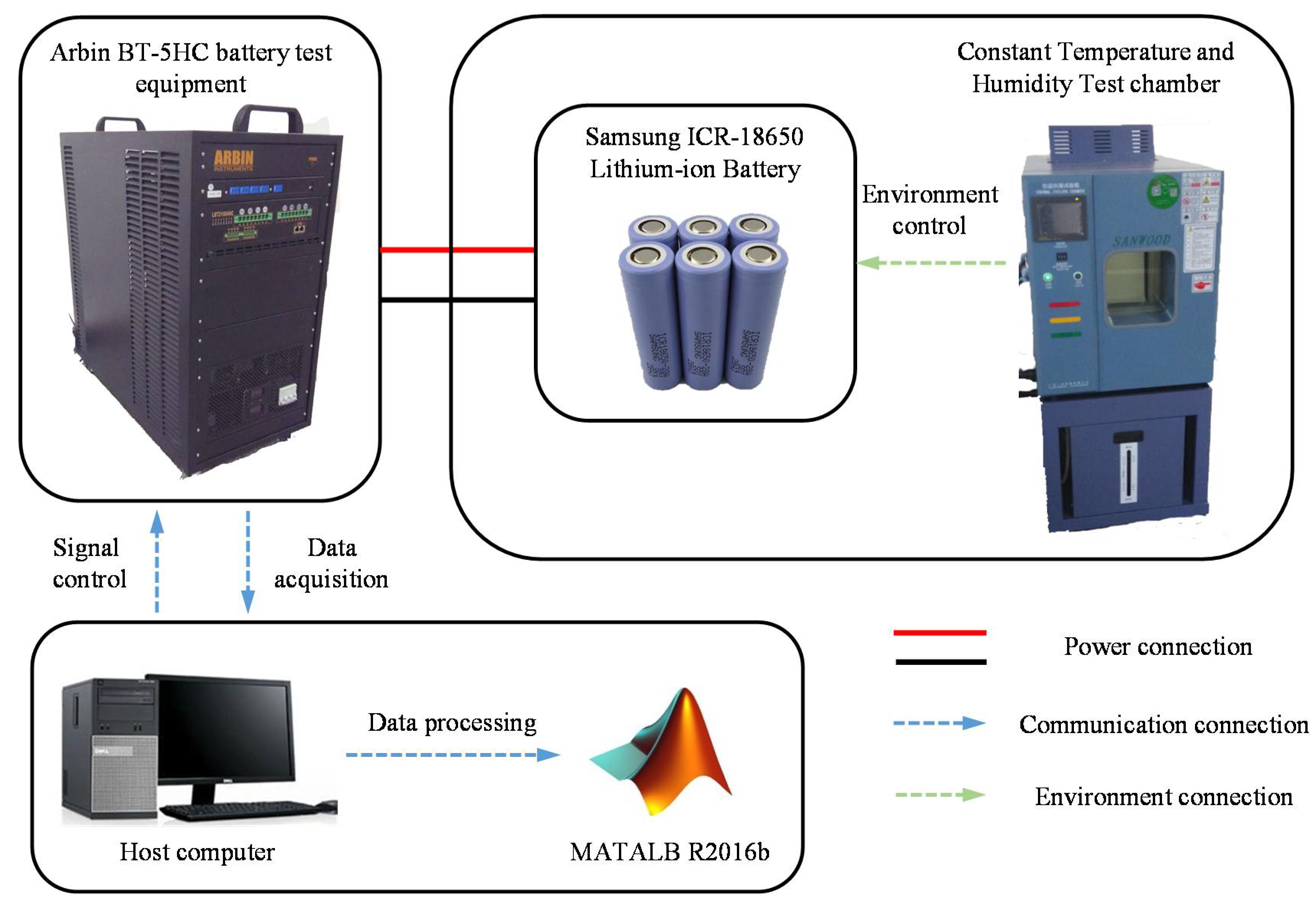
4.1. Test Bench

Figure 3 shows the test bench, which includes Arbin BT-5HC (Arbin, College Station, TX, USA) battery test equipment, a constant temperature and humidity chamber, tested Samsung ICR-18650-22P lithium-ion batteries (Samsung, Seoul, South Korea), and a host computer with MATLAB (R2016b, MathWorks, Natick, MA, USA) installed. The test chamber (Sanwood, Dongguan, China) controls the temperature and humidity environment of tested batteries. The battery test equipment has a voltage range of 5 V, four current ranges of 0.02 A, 0.5 A, 5 A, and 30 A, and measurement accuracy of current and voltage of ± 0.02 % full scale range. The battery test equipment controls the charge and discharge process and transmits the experimental data to the host computer in which the MATLAB is used to conduct the estimation process and analyze the experiment results. The tested batteries have a nominal capacity of 2150 mA, maximum continuous discharging current of 10 A, a nominal voltage of 3.7 V, charging end voltage of 4.2 V, and discharging cut-off voltage of 2.75 V. The set ambient temperature is fixed at 25 °C.

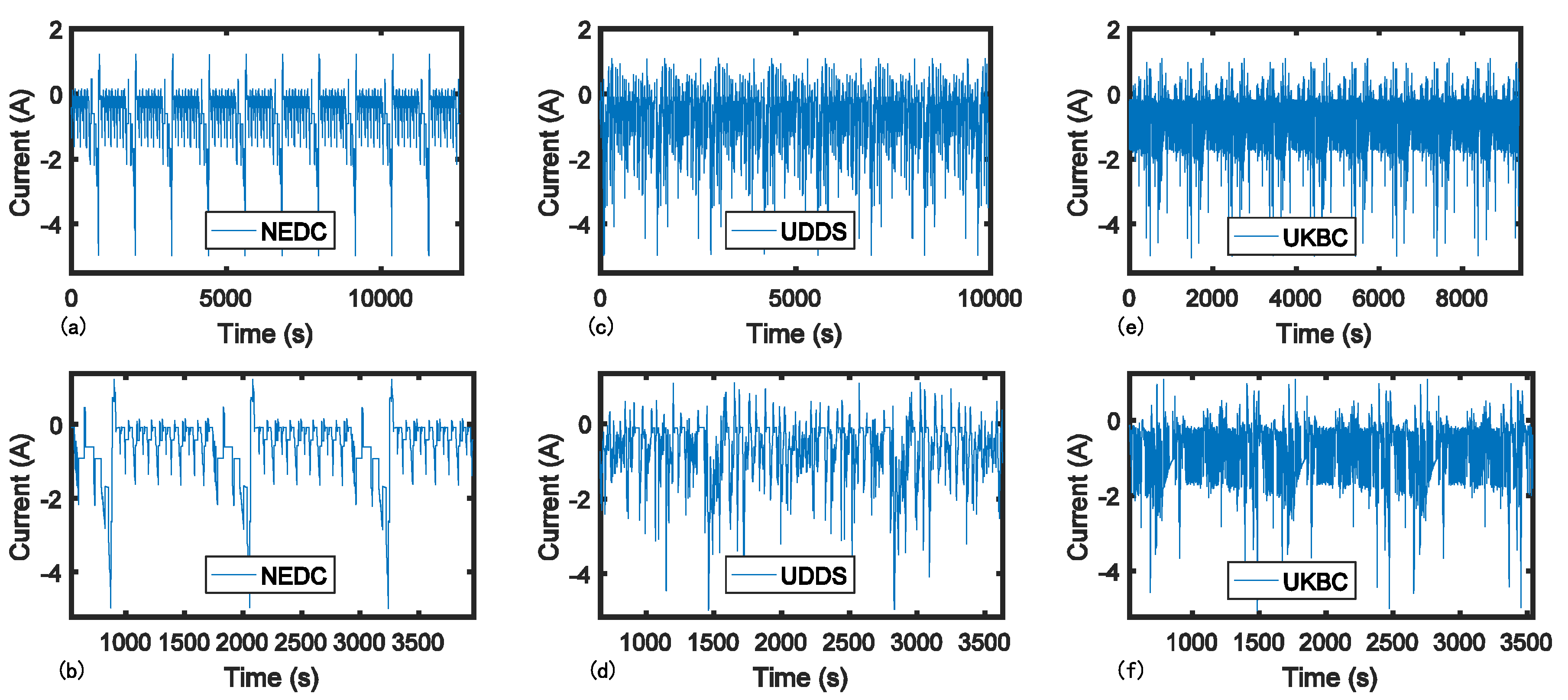
4.2. Data Acquisition

In this paper, based on the experiment directed by the systems analysis tool ADVISOR [51] for EV, NEDC, UDDS (Urban Dynamometer Driving Schedule), and UKBC (the United Kingdom Bus Cycle), three driving cycles are tested, which are shown in Figure 4. The current, voltage, and SOC values are mainly collected in the experiment, and the data under NEDC driving cycle are used as the training data, and the data under the other two cycles are used for discussion sections. The batteries are discharged from 98% to 2% with the battery’s surface temperature in the range from 25.42 °C to 26.48 °C, whose average value is 25.94 °C.

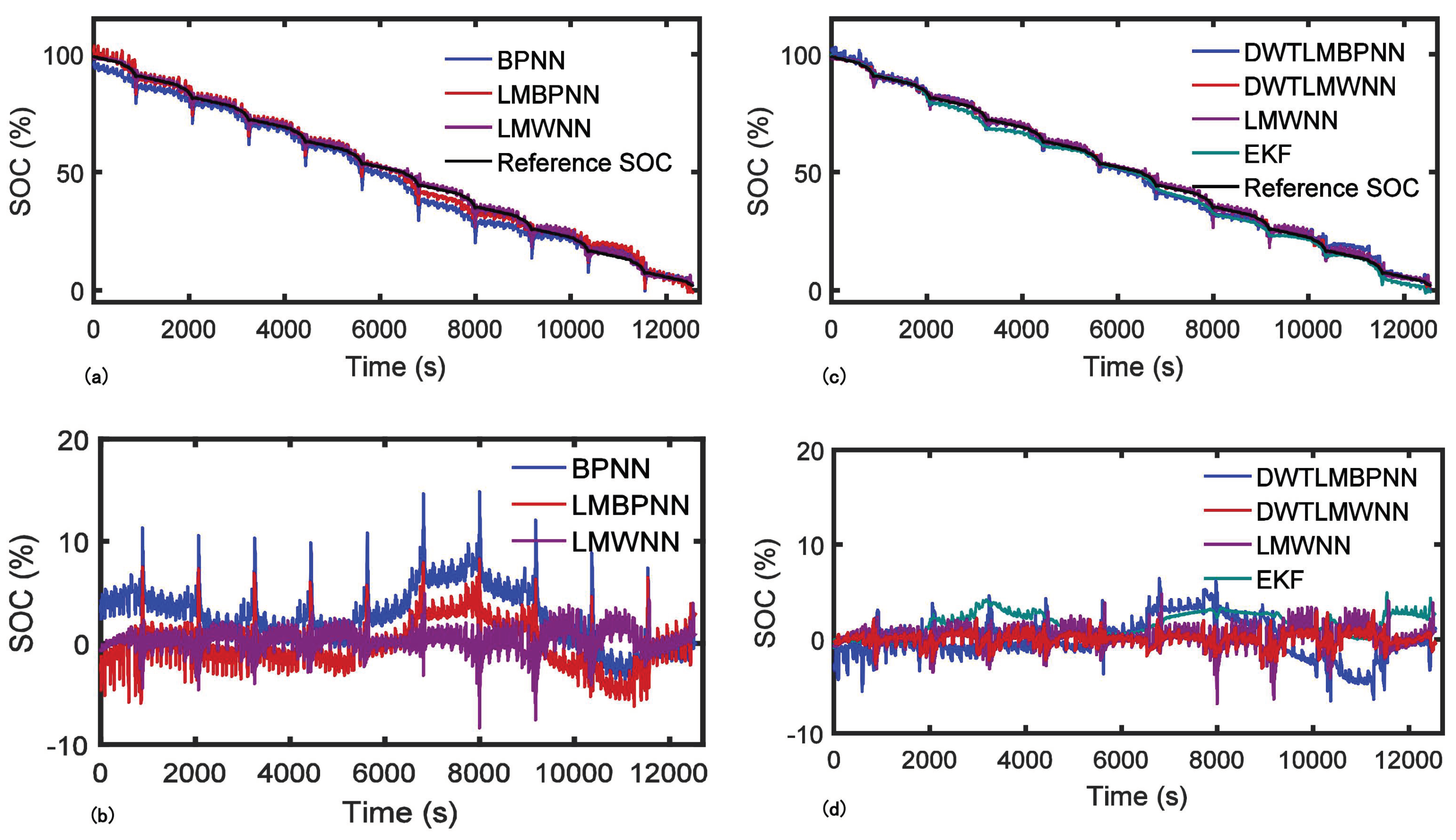
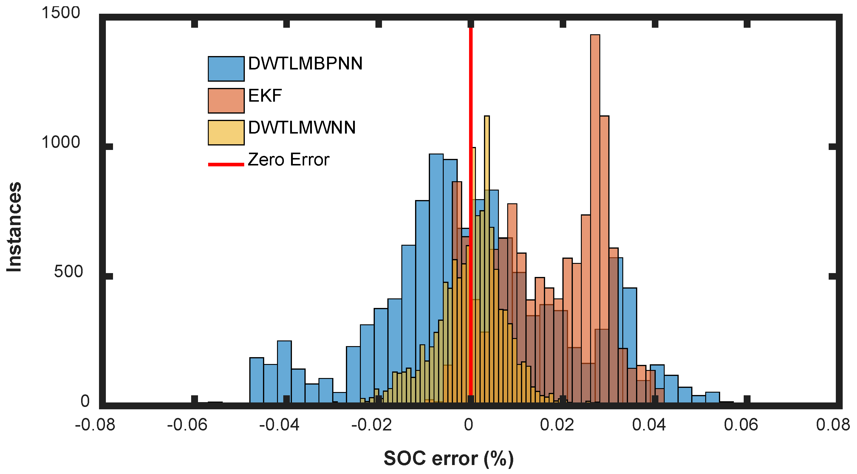
4.3. Method Validation and Comparison Study

In this paper, in order to validate the performance of DWTLMWNN, other SOC estimation methods based on BPNN, L-M-based BPNN (LMBPNN), L-M based WNN (LMWNN), DWT-based LMBPNN (DWTLMBPNN), and EKF are used to make a comparative study. The estimation process of DWT-based WNN is as shown in Figure 1. In order to denoise and keep most useful information, based on a preliminary experiment, the input data of the WNN is set as the reconstructed components x ( n ) A 3 and x ( n ) D 1 of the current and voltage, respectively. The DWT and IDWT processes are conducted in three decomposition levels using the Daubechies basis of order 5 (dB5). The training reconstructed components are normalized into the range of [–1, 1], which are transformed using the following formula:
x m i d = x m a x + x m i n 2 x ' = 2 ( x x m i d ) x m a x x m i n
in which x m a x and x m i n , respectively, denote the maximum value and minimum value of original input variables, and x and x′, respectively, denote original input variable and normalized input variable.
On account of random selection of the initial WNN parameters, the estimation result may possess small fluctuations in the same conditions. The results shown in this paper are the moderate and effective ones. The number of nodes in hidden layer is selected as 10.
As shown in Figure 5 and Table 1, BPNN, LMBPNN, LMWNN, DWTLMBPNN, DWTLMWNN, and EKF are validated under the NEDC. The ANN-based methods in the experiments have the same training data, number of hidden layer nodes, and working environment. The comparative EKF SOC estimation method is based on the second-order equivalent circuit model. The identified parameters and tuning parameters are shown in Table 2. To make the comparison more reasonable, the initial state is set as [1;0;0], while the initial SOC is supposed to be 100%. Thus, the covariance of observation noise Qk is selected to be not very small as a balance.
According to Figure 5b–d, the application of L-M algorithm and DWT method makes effective improvement on the SOC estimation accuracy. Based on the exact values in Table 1, it is found that L-M algorithm reduces the mean absolute error considerably and greatly improves the approximation ability according to the values of the correlation coefficient R but cannot reduce the maximum error to a desired level. DWT method can well reduce the maximum error of SOC estimation. Compared with model-based EKF estimation methods and BPNN-based estimation methods, WNN-based methods have the characteristics of low mean absolute error (e.g., only the mean absolute errors of LMWNN and DWTLMWNN below 1.00%), and the proposed method can solve the high maximum error problem (e.g., the maximum error is reduced more than 5% compared with LMWNN method). Furthermore, according to the results that DWT method reduces the mean absolute error and maximum error of LMBPNN by 0.03% and 1.74%, respectively, but of LMWNN by 0.23% and 5.23%, respectively, it is found that the estimation accuracy improvement using the combination of DWT method and adaptive WNN method is more considerable, which indicates the superiority of the proposed combination method. Figure 6 shows the error histogram of EKF, DWTLMBPNN, and DWTLMWNN, which directly supports that the DWTLMWNN SOC estimation method has advantage of estimation accuracy. Although the training time of ANN-based method is larger than the EKF based method unavoidably according to Table 1, the estimation time of ANN-based method is satisfying, which means the feasibility of actual SOC estimation application.

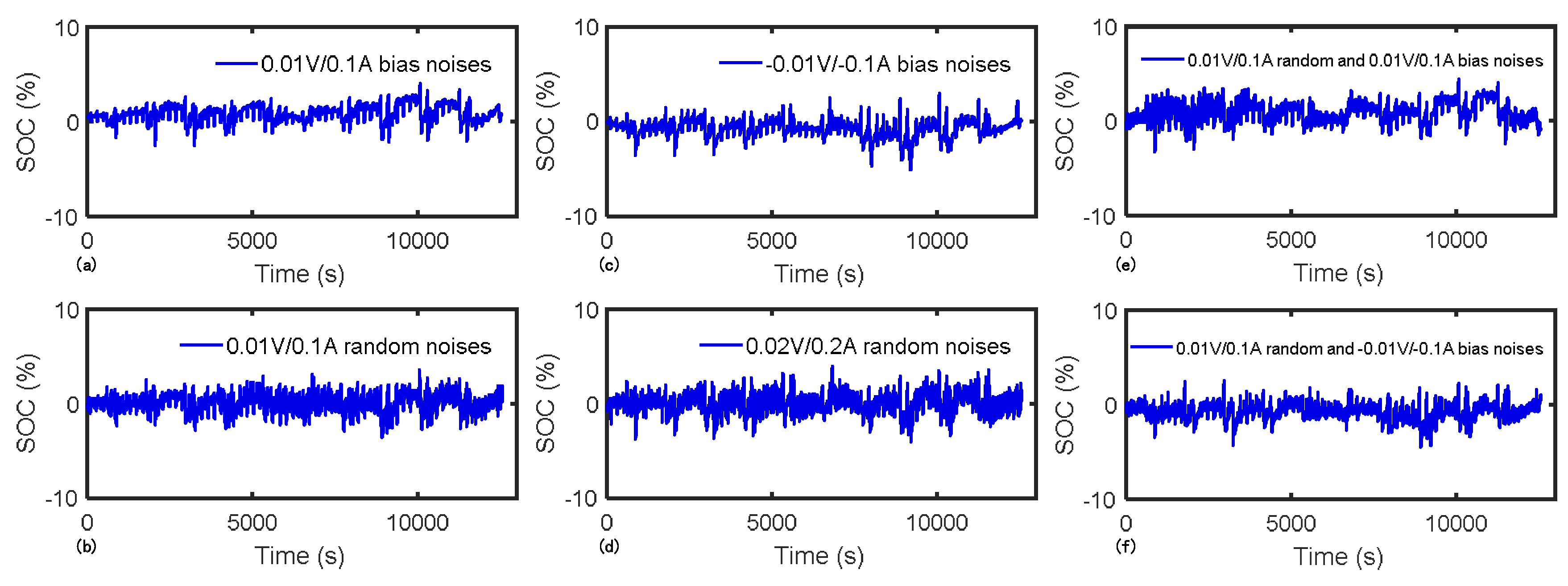
4.4. Robustness Evaluation

Influenced by electromagnetic interference or low precision sensors, the measured input data may not be that accurate. Therefore, noises are simulated as bias noises and random noises added to current and voltage to evaluate the robustness of proposed method. Moreover, different driving cycles have different charge and discharge forms. Therefore, tests on untrained driving cycle for the proposed method should be conducted.

4.4.1. Measurement Noise Test

As shown in Figure 7, the absolute values of positive and negative bias noises added to current and voltage are, respectively, 0.1 A and 0.01 V. The amplitudes of random noises are, respectively, 0.1 A and 0.01 V or 0.2 A and 0.02 V. According to Table 3, compared with EKF SOC estimation method, the DWTLMWNN SOC estimation method has great robustness against noises, especially against large random noises. Besides, the DWTLMWNN method is more stable than the EKF method for the reason that the mean absolute errors and maximum errors of different noise types for the DWTLMWNN method have much less variation, whose mean absolute errors range from 0.66% to 1.16% and maximum errors range from 3.62% to 5.12%, than for the EKF method, whose mean absolute errors range from 1.13% to 3.99% and maximum errors range from 3.32% to 11.44%. The results indicate that the DWTLMWNN method has a good performance against measurement noise and is more stable and accurate than the EKF SOC estimation method.

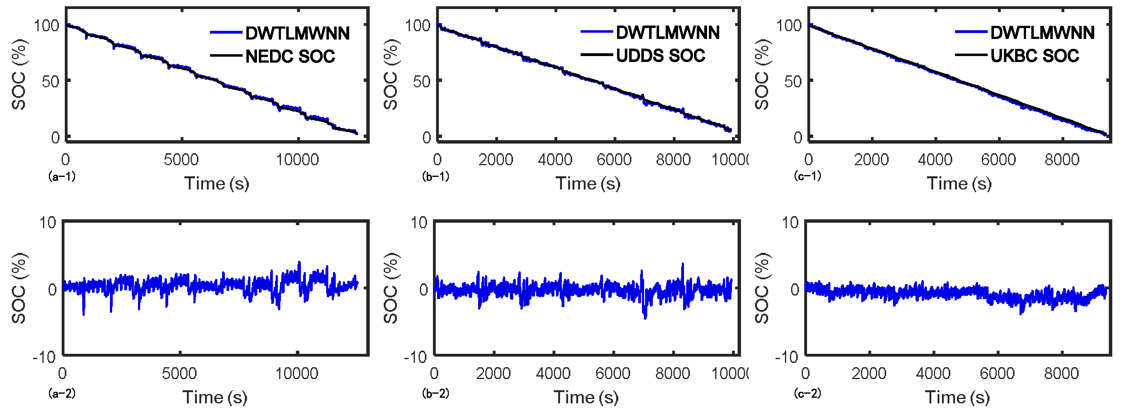
4.4.2. Untrained Driving Cycle Test

In this section, the DWTLMWNN is trained by the data collected under the NEDC and UDDS, and then validated under the UKBC. As shown in Figure 8 and in Table 4, for the trained driving cycles and the untrained driving cycle, the DWTLMWNN SOC estimation method has good estimation performance in terms of the low mean absolute errors and maximum errors. Although the results show that the accuracy of SOC estimation under the NEDC reduces, the overall estimation results are ensured to a satisfying level. Compared with the EKF method, the DWTLMWNN SOC estimation method has a more reliable performance for the unexpected conditions.

5. Conclusions

In this paper, DWTLMWNN, as a hybrid WNN model combining DWT method and adaptive WNN, is proposed to estimate the SOC of lithium-ion batteries. Comparing with BPNN, LMBPNN, LMWNN, DWTLMBPNN, and EKF, the proposed intelligent SOC estimation method is validated and proved to be more effective. The characteristics of high accuracy and strong robustness of the proposed method are verified by a comparison study and robustness evaluation results.
It is found that the proposed analyzed method can solve the high maximum error problem of the BPNN- or WNN-based methods (e.g., the maximum error of DWTLMWNN is reduced to 3.13% under the NEDC). Furthermore, the mean absolute error and maximum error are ensured in a satisfying level even if there is large measurement noise (e.g., 0.2 A/0.02 V random noises) or under untrained driving cycles. Therefore, the proposed method is suitable and of great significance for SOC estimation.
Future work may focus on verifying the proposed method using a high-rate load condition, and the robustness test on packet loss will be considered. Other learning algorithms of neural networks such as the Bayesian regularization method and scaled conjugate gradient will also be employed tentatively in the future. Additionally, the influence of temperature on the proposed method will be studied.

Acknowledgments

This work was supported by the Economic, Trade, and Information Commission Shenzhen of Shenzhen Municipality Strategic Emerging Industries and Future Industrial Development “Innovation Chain + Industrial Chain” Project (2017).

Author Contributions

Bizhong Xia and Deyu Cui proposed the estimation algorithms and designed the comparative experiments; Deyu Cui, Zhen Sun, and Zizhou Lao practically conducted the experiments based on the experiment design; Bizhong Xia, Deyu Cui, and Ruifeng Zhang analyzed the data in MATLAB and obtained the main results of this paper; Wei Wang and Wei Sun provided materials and equipment; Yongzhi Lai and Mingwang Wang gave experimental guidance; and Deyu Cui wrote the paper.

Conflicts of Interest

The authors declare that there is no conflict of interest.

Nomenclature

Acronyms
AAmpere
A·hAmpere-hour
ANNsArtificial neural networks
BMSBattery management system
BPNNBack-propagation neural network
CKFCubature Kalman Filter
DWTDiscrete wavelet transform
DWTLMBPNNDiscrete wavelet transform and Levenberg-Marquardt algorithm-based back-propagation neural network
DWTLMWNNDiscrete wavelet transform and Levenberg-Marquardt algorithm-based wavelet neural network
EKFExtend Kalman filter
EVElectric vehicle
HPPCThe hybrid power pulse characteristics
IDWTInverse discrete wavelet transform
KFKalman filter
L-MLevenberg-Marquardt
LMBPNNLevenberg-Marquardt based back-propagation neural network
LMWNNLevenberg-Marquardt based three-layer wavelet neural network
MATLABMatrix Laboratory
MRAMulti-resolution analysis
NEDCNew European Driving Cycle
OCVOpen-circuit voltage
PFParticle filter
RNNRadial neural network
SMOSliding mode observer
SOCState of charge
SVMSupport vector machine
UDDSUrban Dynamometer Driving Schedule
UKBCthe United Kingdom Bus Cycle
UKFUnscented Kalman filter
VVolt
WNNWavelet neural network
Symbols
aWavelet dilation parameter
A 1 A 3 Approximation components of different levels
bWavelet translation parameter
C1, C2Capacitance values of second-order equivalent circuit model
CnThe nominal capacity of the battery [F]
D 1 D 3 Detail components of different levels
e Error column vector
EThe output mean square error
h Parameters which need to be updated
i/ICurrent [A]
JNumber of decomposition level
J ( h ) Jacobian matrix
K, L or MTotal number of the nodes in input layer, hidden layer, or output layer
netWeighted sum value of a node
NMaximum decomposition level
oOutput data of the neural network
PThe number of total input sets
P0Predicted covariance
QkCovariance of observation noise
RThe correlation coefficient
R0, R1, R2Resistance values of second-order equivalent circuit model
RkCovariance of process noise
tTime [s]
t0Initial time [s]
UCell voltage or cell potential [V]
V The total output mean square error
x Input data of the neural network
x ' Output data of the hidden layer
x ( t ) The original signal
β , μ Tuning parameters of Levenberg-Marquardt algorithm
δ Equivalent error in the steepest descent algorithm
Δ Equivalent error in the Levenberg-Marquardt algorithm
ψ ( t ) Mother wavelet function
ϕ ( t ) Scaling function
ω Weight of neural networks between input and hidden layer
ω ' Weight of neural networks between hidden and output layer
Subscript
minMinimum value
maxMaximum value
k, l or mNumber of the nodes in input layer, hidden layer, or output layer
j, k in DWTDilation parameter and translation parameter
Superscript
Values of hidden layer related to output layer
Values of output layer
* Updated value or complex conjugate
( 1 ) First derivative
Abbreviations
meanMean absolute error
maxMaximum absolute error
maximum errorMaximum absolute error

References

  1. Zhang, Z.L.; Cheng, X.; Lu, Z.Y.; Gu, D.J. SOC Estimation of Lithium-Ion Batteries with AEKF and Wavelet Transform Matrix. IEEE Trans. Power Electr. 2017, 32, 7626–7634. [Google Scholar] [CrossRef]
  2. Srivastav, S.; Lacey, M.J.; Brandell, D. State-of-charge indication in Li-ion batteries by simulated impedance spectroscopy. J. Appl. Electrochem. 2017, 47, 229–236. [Google Scholar] [CrossRef]
  3. Tian, Y.; Li, D.; Tian, J.D.; Xia, B.Z. State of charge estimation of lithium-ion batteries using an optimal adaptive gain nonlinear observer. Electrochim. Acta 2017, 225, 225–234. [Google Scholar] [CrossRef]
  4. Panchal, S.; Dincer, I.; Agelin-Chaab, M.; Fraser, R.; Fowler, M. Thermal modeling and validation of temperature distributions in a prismatic lithium-ion battery at different discharge rates and varying boundary conditions. Appl. Therm. Eng. 2016, 96, 190–199. [Google Scholar] [CrossRef]
  5. Ng, K.S.; Moo, C.S.; Chen, Y.P.; Hsieh, Y.C. Enhanced coulomb counting method for estimating state-of-charge and state-of-health of lithium-ion batteries. Appl. Energy 2009, 86, 1506–1511. [Google Scholar] [CrossRef]
  6. Yang, N.X.; Zhang, X.W.; Li, G.J. State of charge estimation for pulse discharge of a LiFePO4 battery by a revised Ah counting. Electrochim. Acta 2015, 151, 63–71. [Google Scholar] [CrossRef]
  7. Lee, S.; Kim, J.; Lee, J.; Cho, B.H. State-of-charge and capacity estimation of lithium-ion battery using a new open-circuit voltage versus state-of-charge. J. Power Sources 2008, 185, 1367–1373. [Google Scholar] [CrossRef]
  8. Panchal, S.; Dincer, I.; Agelin-Chaab, M.; Fraser, R.; Fowler, M. Experimental and theoretical investigations of heat generation rates for a water cooled LiFePO4 battery. Int. J. Heat Mass Transf. 2016, 101, 1093–1102. [Google Scholar] [CrossRef]
  9. Lee, J.; Nam, O.; Cho, B.H. Li-ion battery SOC estimation method based on the reduced order extended Kalman filtering. J. Power Sources 2007, 174, 9–15. [Google Scholar] [CrossRef]
  10. Yuan, S.F.; Wu, H.J.; Yin, C.L. State of Charge Estimation Using the Extended Kalman Filter for Battery Management Systems Based on the ARX Battery Model. Energies 2013, 6, 444–470. [Google Scholar] [CrossRef]
  11. Xiong, B.; Zhao, J.; Wei, Z.; Skyllas-Kazacos, M. Extended Kalman filter method for state of charge estimation ofvanadium redox flow battery using thermal-dependent electrical model. J. Power Sources 2014, 262, 50–61. [Google Scholar] [CrossRef]
  12. Santhanagopalan, S.; White, R.E. Online estimation of the state of charge of a lithium ion cell. J. Power Sources 2006, 161, 1346–1355. [Google Scholar] [CrossRef]
  13. He, W.; Williard, N.; Chen, C.C.; Pecht, M. State of charge estimation for electric vehicle batteries using unscented kalman filtering. Microelectron. Reliab. 2013, 53, 840–847. [Google Scholar] [CrossRef]
  14. He, Z.G.; Chen, D.; Pan, C.F.; Chen, L.; Wang, S.H. State of charge estimation of power Li-ion batteries using a hybrid estimation algorithm based on UKF. Electrochim. Acta 2016, 211, 101–109. [Google Scholar]
  15. Kim, I.S. The novel state of charge estimation method for lithium battery using sliding mode observer. J. Power Sources 2006, 163, 584–590. [Google Scholar] [CrossRef]
  16. Chen, X.P.; Shen, W.X.; Cao, Z.W.; Kapoor, A. A novel approach for state of charge estimation based on adaptive switching gain sliding mode observer in electric vehicles. J. Power Sources 2014, 246, 667–678. [Google Scholar] [CrossRef]
  17. Lotfi, N.; Landers, R.G.; Li, J.; Park, J. Reduced-Order Electrochemical Model-Based SOC Observer with Output Model Uncertainty Estimation. IEEE Trans. Control Syst. Technol. 2017, 25, 1217–1230. [Google Scholar] [CrossRef]
  18. Dey, S.; Ayalew, B.; Pisu, P. Nonlinear Robust Observers for State-of-Charge Estimation of Lithium-Ion Cells Based on a Reduced Electrochemical Model. IEEE Trans. Control Syst. Technol. 2015, 23, 1935–1942. [Google Scholar] [CrossRef]
  19. Zou, C.F.; Manzie, C.; Nesic, D.; Kallapur, A.G. Multi-time-scale observer design for state-of-charge and state-of-health of a lithium-ion battery. J. Power Sources 2016, 335, 121–130. [Google Scholar] [CrossRef]
  20. Schwunk, S.; Armbruster, N.; Straub, S.; Kehl, J.; Vetter, M. Particle filter for state of charge and state of health estimation for lithium-iron phosphate batteries. J. Power Sources 2013, 239, 705–710. [Google Scholar] [CrossRef]
  21. Wang, Y.J.; Zhang, C.B.; Chen, Z.H. A method for state-of-charge estimation of LiFePO4 batteries at dynamic currents and temperatures using particle filter. J. Power Sources 2015, 279, 306–311. [Google Scholar] [CrossRef]
  22. Li, Z.; Huang, J.; Liaw, B.Y.; Zhang, J. On state-of-charge determination for lithium-ion batteries. J. Power Sources 2017, 348, 281–301. [Google Scholar] [CrossRef]
  23. Sepasi, S.; Ghorbani, R.; Liaw, B.Y. Inline state of health estimation of lithium-ion batteries using state of charge calculation. J. Power Sources 2015, 299, 246–254. [Google Scholar] [CrossRef]
  24. Andre, D.; Meiler, M.; Steiner, K.; Walz, H.; Soczka-Guth, T.; Sauer, D.U. Characterization of high-power lithium-ion batteries by electrochemical impedance spectroscopy. II: Modelling. J. Power Sources 2011, 196, 5349–5356. [Google Scholar] [CrossRef]
  25. Wei, Z.B.; Zou, C.F.; Leng, F.; Soong, B.H.; Tseng, K.J. Online Model Identification and State-of-Charge Estimate for Lithium-Ion Battery With a Recursive Total Least Squares-Based Observer. IEEE Trans. Ind. Electron. 2018, 65, 1336–1346. [Google Scholar] [CrossRef]
  26. Zou, C.F.; Hu, X.S.; Wei, Z.B.; Tang, X.L. Electrothermal dynamics-conscious lithium-ion battery cell-level charging management via state-monitored predictive control. Energy 2017, 141, 250–259. [Google Scholar] [CrossRef]
  27. Cheng, B.; Bai, Z.F.; Cao, B.G. State of charge estimation based on evolutionary neural network. Energy Convers. Manag. 2008, 49, 2788–2794. [Google Scholar]
  28. Dang, X.J.; Yan, L.; Xu, K.; Wu, X.R.; Jiang, H.; Sun, H.X. Open-Circuit Voltage-Based State of Charge Estimation of Lithium-ion Battery Using Dual Neural Network Fusion Battery Model. Electrochim. Acta 2016, 188, 356–366. [Google Scholar] [CrossRef]
  29. Sbarufatti, C.; Corbetta, M.; Giglio, M.; Cadini, F. Adaptive prognosis of lithium-ion batteries based on the combination of particle filters and radial basis function neural networks. J. Power Sources 2017, 344, 128–140. [Google Scholar] [CrossRef]
  30. Hansen, T.; Wang, C.J. Support vector based battery state of charge estimator. J. Power Sources 2005, 141, 351–358. [Google Scholar] [CrossRef]
  31. Zhou, P.W.; Wang, L.J.; Lin, H.P.; Lv, Z.Y. High Accuracy State-of-Charge Online Estimation of EV/HEV Lithium Batteries Based on Adaptive Wavelet Neural Network. In Proceedings of the 2013 IEEE ECCE Asia Downunder (Ecce Asia), Melbourne, VIC, Australia, 3–6 June 2013; pp. 513–517. [Google Scholar]
  32. Gao, L.; Song, Y.; Dougal, R.A. Wavelet neural network based battery state-of-charge estimation for portable electronics applications. In Proceedings of the Twentieth Annual IEEE Applied Power Electronics Conference and Exposition, Austin, TX, USA, 6–10 March 2005; Volume 2, pp. 998–1002. [Google Scholar]
  33. Rivera-Barrera, J.P.; Munoz-Galeano, N.; Sarmiento-Maldonado, H.O. SoC Estimation for Lithium-ion Batteries: Review and Future Challenges. Electronics 2017, 6, 102. [Google Scholar] [CrossRef]
  34. Chen, H.Y.; Liang, J.W. Adaptive Wavelet Neural Network Controller for Active Suppression Control of a Diaphragm-type Pneumatic Vibration Isolator. Int. J. Control Autom. Syst. 2017, 15, 1456–1465. [Google Scholar] [CrossRef]
  35. Jiao, Z.; Zhang, R. Fault Diagnosis Based on Multi-layer Structure Wavelet Neural Networks in Attitude Heading Reference System. Adv. Dev. Eng. Sci. IV 2014, 1046, 270–274. [Google Scholar] [CrossRef]
  36. Wei, S.K.; Yang, H.; Song, J.X.; Abbaspour, K.; Xu, Z.X. A wavelet-neural network hybrid modelling approach for estimating and predicting river monthly flows. Hydrol. Sci. J. 2013, 58, 374–389. [Google Scholar] [CrossRef]
  37. Liu, Z.G.; Wang, Q.; Zhang, Y.J. Combining Multi Wavelet and Multi NN for Power Systems Load Forecasting. In Proceedings of the 5th International Symposium on Neural Networks (ISNN 2008, Ptart 2), Beijing, China, 24–28 September 2008; Volume 5264, pp. 666–673. [Google Scholar]
  38. Zhang, J.; Gao, X.P.; Li, Y.Q. Efficient wavelet networks for function learning based on adaptive wavelet neuron selection. IET Signal Process. 2012, 6, 79–90. [Google Scholar] [CrossRef]
  39. Szu, H.H.; Telfer, B.; Kadambe, S. Neural Network Adaptive Wavelets for Signal Representation and Classification. Opt. Eng. 1992, 31, 1907–1916. [Google Scholar] [CrossRef]
  40. Lee, S.; Kim, J. Discrete wavelet transform-based denoising technique for advanced state-of-charge estimator of a lithium-ion battery in electric vehicles. Energy 2015, 83, 462–473. [Google Scholar] [CrossRef]
  41. Kim, J.; Chun, C.Y.; Cho, B.H. Implementation of EKF combined with Discrete Wavelet Transform-based MRA for Improved SOC Estimation for a Li-Ion Cell. In Proceedings of the 2013 Twenty-Eighth Annual IEEE Applied Power Electronics Conference and Exposition (APEC), Long Beach, CA, USA, 17–21 March 2013; pp. 2720–2725. [Google Scholar]
  42. Kim, J.; Cho, B.H. Application of Wavelet Transform-based Discharging/Charging Voltage Signal Denoising for Advanced Data-Driven SOC Estimator. In Proceedings of the 2015 IEEE Applied Power Electronics Conference and Exposition (APEC), Charlotte, NC, USA, 15–19 March 2015; pp. 3013–3018. [Google Scholar]
  43. Kim, J. Cell Seletion through Two-Level Basis Pattern Recognition with Low/High Frequency Components Decomposed by DWT-based MRA. In Proceedings of the 2014 IEEE Energy Conversion Congress and Exposition (ECCE), Pittsburgh, PA, USA, 14–18 September 2014; pp. 906–911. [Google Scholar]
  44. Tarbi, A.; Atmani, E.H.; Sellam, M.A. Control and diagnostic of the complex impedance of selected perovskite compounds. Opt. Quant. Electron. 2017, 49, 337. [Google Scholar] [CrossRef]
  45. Das, P.P.; Bisoi, R.; Dash, P.K. Time Series Forecasting Using Fuzzy Functional Link Neural Network Trained By Improved Second Order Levenberg-Marquardt Algorithm. In Proceedings of the 2015 IEEE Power, Communication and Information Technology Conference (PCITC), Bhubaneswar, India, 15–17 October 2015; pp. 827–833. [Google Scholar]
  46. Kumar, A.; Kumar, R. Least Square Fitting for Adaptive Wavelet Generation and Automatic Prediction of Defect Size in the Bearing Using Levenberg-Marquardt Backpropagation. J. Nondestruct. Eval. 2017, 36, 7. [Google Scholar] [CrossRef]
  47. Hu, P.; Cao, G.Y.; Zhu, X.J.; Li, J. Modeling of a proton exchange membrane fuel cell based on the hybrid particle swarm optimization with Levenberg-Marquardt neural network. Simul. Model. Pract. Theory 2010, 18, 574–588. [Google Scholar] [CrossRef]
  48. Kim, J. Discrete Wavelet Transform-Based Feature Extraction of Experimental Voltage Signal for Li-Ion Cell Consistency. IEEE Trans. Veh. Technol. 2016, 65, 1150–1161. [Google Scholar] [CrossRef]
  49. Sang, Y.F.; Sun, F.B.; Singh, V.P.; Xie, P.; Sun, J. A discrete wavelet spectrum approach for identifying non-monotonic trends in hydroclimate data. Hydrol. Earth Syst. Sci. 2018, 22, 757–766. [Google Scholar] [CrossRef]
  50. Kim, J.; Cho, B.H. An innovative approach for characteristic analysis and state-of-health diagnosis for a Li-ion cell based on the discrete wavelet transform. J. Power Sources 2014, 260, 115–130. [Google Scholar] [CrossRef]
  51. Markel, T.; Brooker, A.; Hendricks, I.; Johnson, V.; Kelly, K.; Kramer, B.; O’Keefe, M.; Sprik, S.; Wipke, K. ADVISOR: A systems analysis tool for advanced vehicle modeling. J. Power Sources 2002, 110, 255–266. [Google Scholar] [CrossRef]
Figure 1. Structure of a three-layer WNN.
Energies 11 00995 g001
Figure 2. Structure of a three-level, DWT-based decomposition and reconstruction processes and DWT-WNN-based SOC estimation process.
Energies 11 00995 g002
Figure 3. Structure of battery test bench.
Energies 11 00995 g003
Figure 4. Current profiles and zoom figure of (a,b) NEDC, (c,d) UDDS, and (e,f) UKBC.
Energies 11 00995 g004
Figure 5. SOC estimation and SOC error under the NEDC: (a,b) BPNN, LMBPNN, and LMWNN; (c,d) DWTLMBPNN, DWTLMWNN, LMWNN, and EKF.
Energies 11 00995 g005
Figure 6. SOC estimation error histogram using DWTLMBPNN, EKF, and DWTLMWNN under the NEDC.
Energies 11 00995 g006
Figure 7. SOC estimation with measurement noises under the NEDC.
Energies 11 00995 g007
Figure 8. SOC estimation and SOC error under: (a–1,a–2) NEDC (trained), (b–1,b–2) UDDS (trained), and (c–1,c–2) UKBC (untrained).
Energies 11 00995 g008
Table 1. Mean and maximum SOC error of BPNN, LMBPNN, LMWNN, DWTLMBPNN, DWTLMWNN, and EKF.
MethodsBPNNLMBPNNLMWNNDWT LMBPNNDWT LMWNNEKF
Mean absolute error3.22%1.69%0.82%1.65%0.59%1.71%
Maximum error14.84%8.28%8.36%6.54%3.13%5.17%
R0.949370.997480.999620.997160.999670.97871
Estimation time0.0772 s0.0947 s0.1362 s0.2328 s0.2461 s0.3276 s
Training time12.8785 s6.0839 s13.6264 s6.2151 s13.7539 s-
Table 2. Identified parameters and tuning parameters of the comparative EKF estimation method.
ParametersR0R1R2C1C2
Values0.0377 Ω0.0242 Ω0.0030 Ω1.6733 × 10³ F1.7823 × 105 F
ParametersRkQkP0
Values0.01diag (0.001,0.0001,0.0001)diag (0.01,0.01,0.01)
Table 3. Mean and maximum SOC error with measurement noise under the NEDC.
Noise TypeDWTLMWNN (Mean/Max)EKF (Mean/Max)
0.01 V/0.1 A bias noises1.02%/4.09%1.13%/3.32%
−0.01 V/−0.1 A bias noises0.97%/5.12%3.90%/6.97%
0.01 V/0.1 A random noises0.66%/3.62%2.05%/5.71%
0.02 V/0.2 A random noises0.78%/4.09%3.61%/11.44%
0.01 V/0.1 A random and 0.01 V/0.1 A bias noises1.16%/4.46%1.14%/4.74%
0.01 V/0.1 A random and −0.01 V/−0.1 A bias noises0.92%/4.50%3.99%/9.13%
Table 4. Mean and maximum SOC error of DWTLMWNN and EKF under NEDC, UDDS, and UKBC.
Driving CyclesNEDC (Mean/Max)UDDS (Mean/Max)UKBC (Mean/Max)
DWTLMWNN0.72%/3.95%0.71%/4.50%0.92%/3.83%
EKF1.71%/5.17%2.06%/4.61%2.43%/7.68%

