A Method for Distributed Control of Reactive Power and Voltage in a Power Grid: A Game-Theoretic Approach

1
Electrical & Computer Engineering, Texas A&M University, College Station, TX 77840, USA
2
Electrical & Computer Engineering, Seattle University, Seattle, WA 98122, USA
3
Electrical Engineering, Tuskegee University, Tuskegee, AL 36088, USA
*
Author to whom correspondence should be addressed.
Energies 2018, 11(4), 962; https://doi.org/10.3390/en11040962
Submission received: 24 February 2018
/
Revised: 13 April 2018
/
Accepted: 15 April 2018
/
Published: 17 April 2018
(This article belongs to the Special Issue Control and Communication in Distributed Generation Systems)
Abstract
:The efficiency of a power system is reduced when voltage drops and losses occur along the distribution lines. While the voltage profile across the system buses can be improved by the injection of reactive power, increased line flows and line losses could result due to uncontrolled injections. Also, the determination of global optimal settings for all power-system components in large power grids is difficult to achieve. This paper presents a novel approach to the application of game theory as a method for the distributed control of reactive power and voltage in a power grid. The concept of non-cooperative, extensive = form games is used to model the interaction among power-system components that have the capacity to control reactive power flows in the system. A centralized method of control is formulated using an IEEE 6-bus test system, which is further translated to a method for distributed control using the New England 39-bus system. The determination of optimal generator settings leads to an improvement in load-voltage compliance. Finally, renewable-energy (reactive power) sources are integrated to further improve the voltage-compliance level.
1. Introduction
A major problem experienced by rapidly expanding power systems is the cascade effect that occurs as a result of faults, which calls for an effective coordination process to control such power systems [1,2]. Based on different criteria that include geographical and organizational considerations, large interconnected systems can be decoupled into areas whereby each area can be controlled systematically [3].
Reactive power and voltage support in a power grid are important considerations in power-system stability [4,5]. Voltage collapse is the effect of continuous deterioration of system voltage due to increased loadings, heavy reactive power flows, insufficient reactive power, loss of generation, and other significant events in the system [6,7,8]. Excessive injections of reactive power to improve system voltage could lead to further increases in line loadings and overall line losses. By decoupling large systems, the reactive power–voltage relationship can be better monitored.
The determination of optimal settings for power-system components in large power grids also poses a major challenge [1,9,10] for system control, and hence the ability to decouple large systems into smaller regions will provide a better means for control. Since a global solution of system settings satisfying all constraints is difficult to achieve, the system is sectionalized in order to monitor and determine these settings. The result is a better snapshot of the system voltage given individual area controls.
Procurement of reactive power and control of voltage are issues that are crucial in power systems [10], and several methods have been studied to address the problem of reactive power dispatch. These range from classical methods of optimization, which include non-linear programming (NLP), successive linear programming, mixed integer programming, Newton’s and quadratic techniques [11,12] to evolutionary algorithms, which include artificial neural networks, micro-genetic algorithm [12] and particle swarm optimization [13].
In this paper, a novel application of a game-theoretic (GT) technique is proposed to carry out a method for distributed control in a power grid, using the New England 39-bus system. This work begins by carrying out a means of centralized, systematic voltage and reactive power control in an IEEE 6-bus system, and later evolves to distributed control in the 39-bus system, while optimizing the settings of power-system components. This paper has been organized as follows: an overview of game theory and a study of the reactive power contributions of power-system components are presented in Section 2 and Section 3, respectively; the centralized game model is discussed in Section 4. The proposed game-theoretic equations and algorithms are introduced in Section 5. Expansion of the work into distributed control game model is presented in Section 6, with the integration of distributed renewable energy sources in Section 7. Simulation results and conclusions are presented in Section 8 and Section 9, respectively.
2. Game Theory Overview
Game theory is the study of complex and varied interactions that exist among independent, rational-thinking players [14,15] i.e., the determination of an optimal solution in a multi-variable system controlled by different entities. There are three aspects to each game: players (or agents), actions, and payoff [14,15,16]. Players are the decision makers; actions are the choices available to a player, and a payoff is that utility a player receives for taking an action arising from a chosen strategy [16].
In layman’s terms, game theory revolves around the actions that players take knowing that their decisions affect others [16]. Mathematical formulations can also be used to study these complex interactions [14]. The rationality of a player is defined as its ability to select an optimal action after taking into consideration its available preferences and the expectations about unknowns [15]. Over the years, game theory has evolved from classical to modern and, finally, to new game theory [17]. This evolution hinged on the player’s sense of rationality: a player considers only itself as rational and assumes others as irrational; followed by a rational player considering other players as rational entities; and finally, players forming beliefs about other players’ actions based on a historical trend [17].
In most games, the goal is the attainment of a system equilibrium whereby all players have no incentive to deviate from the strategies (that define their choice of actions) they have individually chosen [14,17]. This scenario, known as, the ‘Nash equilibrium’ is largely credited to John Nash after his contribution in 1951 [18].
Game theory has two broad classifications: Cooperative and non-cooperative games. Cooperative games consider the coalitions that players could form in order to improve their distributed utilities or payoffs. The non-cooperative game focuses on the individual player’s ability to improve its payoff considering the actions of others. Non-cooperative games are further classified into strategic and extensive form games. In the strategic form game, players carry out their actions simultaneously without having knowledge of the previous actions of other players [14,15]. In an extensive form game, players carry out actions in a defined sequence, in which case, players have a knowledge of some or all (i.e., perfect or imperfect information) of the actions previously carried out by others.
2.1. Terminologies
- Nash equilibrium: this captures a steady state of play of a game in which each player holds the correct expectation about the other player’s behavior and acts rationally [15]. It states that all players are, individually, playing their best responses to the actions of others [14]. There is no incentive for any player to deviate.
- Subgame: given perfect information, extensive-form game G, the subgame of G at node h is the restriction of G to the descendants of h [14]. The subgame is a part of the overall extensive game tree, with the overall game tree being the largest subgame. Leyton-Brown and Shoham [14] state requirements to be satisfied for a game to be called a subgame.
- Backward induction: this is an important solution concept utilized in solving extensive form games. By determining the equilibrium play of a lower subgame, further analysis can be carried out until one arrives at the top or root of the tree. According to Shoham and Leyton, it is based on the assumption that that subgame equilibrium will be played as one backs up the tree. This concept is used to arrive at a final solution.
- Subgame perfect equilibrium: these are all strategy profiles, S, such that for any subgame G’ of G, the restriction of S to G’ is a Nash equilibrium of G’ [14]. The direct implication of this is that at every point in history, a player’s strategy is always optimal. Hence, for every strategy profile in history, a state of Nash equilibrium is always achieved. This notion eliminates several Nash equilibria wherein players’ threats are not credible [15].
2.2. Mathematical Representations
- Normal form game: a finite, n-person game is a tuple defined as:N = Set of n number of players, indexed by i.A = A1 × …An, Ai set of actions available to player i.U = (U1…Un), Ui: A→R is a real-valued quantity (or payoff function) for player i.
- Extensive form game: a perfect-information game is defined as:H = set of non-terminal choice nodes. (A choice node is that stage of a game where a player makes a strategic decision on available options).Z = set of terminal nodes, disjoint from H.H→2A is the action function, which assigns to each choice node a set of possible actions.H→N is the player function, which assigns to each non-terminal node player i who chooses an action at that node.H × A→H ∪ Z is the successor function mapping a choice node and an action to a new choice node or terminal node.
3. Reactive Power Contributions of Power System Components
The reactive power contributions of each component (now known as a player) in the power system [19,20] are stated in the sub-sections below:
3.1. Generator
At a generator bus gk, the reactive power injected is given by
where
- = reactive power injection into generator bus gk;
- N = number of buses;
- , = voltages at buses gk and n;
- = admittance matrix entry between buses gk and n;
- = phase angle of the admittance matrix entry between buses gk and n; and
- , = phase angles at buses n and gk.
3.2. Tap-Changing Transformer
The amount of complex powers flowing from buses n to k (Snk) and from k to n (Skn), respectively, are given by:
where t = real part of transformer tap ratio; = is the admittance matrix entry for line connecting bus n and k; = voltage at bus k.
The corresponding reactive powers flowing across the transformer branch are given by:
where δkn = phase angle between buses k and n.
Hence, the average amount of reactive power flowing across the transformer branch is given by:
3.3. Shunt Reactive Compensator
The amount of reactive power injected, , is in discrete steps based on the given step size. Within its range of control (–), the compensator is able to support the system.
4. Centralized Game Model
In order to carry out distributed control, a game-theoretic scheme was first formulated to implement centralized control [20]. The game definition for centralized control is stated in the sub-sections below.
4.1. Objectives
This refers to the parameters that are meant to be optimized in the game. In our game model, reactive power and voltage control are the two main objectives. Specifically, they are to ensure minimal contribution of reactive power to the system during voltage control.
4.2. Players
Players in a game are agents or entities that perform a set of actions to achieve the aforementioned objectives. In our game model, players are the generators, on-load tap changing transformers (OLTCs), and reactive power shunt compensating devices.
4.3. Actions
The strategies employed by players in order to achieve the objectives of the game are called actions. In our game model, this refers to the different possible settings that players can choose during voltage control. Specifically, the settings of the generator’s automatic voltage regulator (AVR), OLTC tap, and reactive power injection from shunt compensators, are all considered to vary in discrete steps.
4.4. Payoffs
This refers to the incentives earned by players as a result of taking actions to meet the desired objectives. In our game model, these are the average amounts of reactive power flowing along the OLTC-connected branch, and reactive power injections from the generators and compensators.
4.5. Payoff Vector
A vector that shows the payoffs for all players for any action combination or strategy profile.
4.6. Power-Flow Equations
These are the power-flow equations for real and reactive power injections to be solved at bus k, and are given by:
4.7. Constraints
- Equality constraints: this defines the amount of power being injected into a bus [11]:where and are the real and reactive powers injected into bus k, respectively; and are the real and reactive powers absorbed by the load connected at bus k, respectively; and and are the real and reactive powers injected into the line at bus k, respectively.
- Inequality constraints: these define the lower and upper limits of operation of the components and system specifications [11]:where is the generator reactive power input; is the AVR setting of the generator; is the transformer tap setting; is the value of the shunt reactive power compensator; and is the voltage at the load buses. These values are all defined within their operating lower and upper limits.
4.8. Power-System Model
4.9. Centralized Game-Theoretic Model
The non-cooperative form game model was chosen to reflect the hierarchical interactions of the power-system components, and to propose a systematic method for reactive power control.
Hierarchy of control: an order of control was defined to develop the tree diagram arising from the extensive form game. Based on actual practice in which generators have the smallest time constants, the order considered was generator–OLTC–compensator. This implies that, upon request for control action, the generator acts first, followed by the OLTC, and finally the compensator.
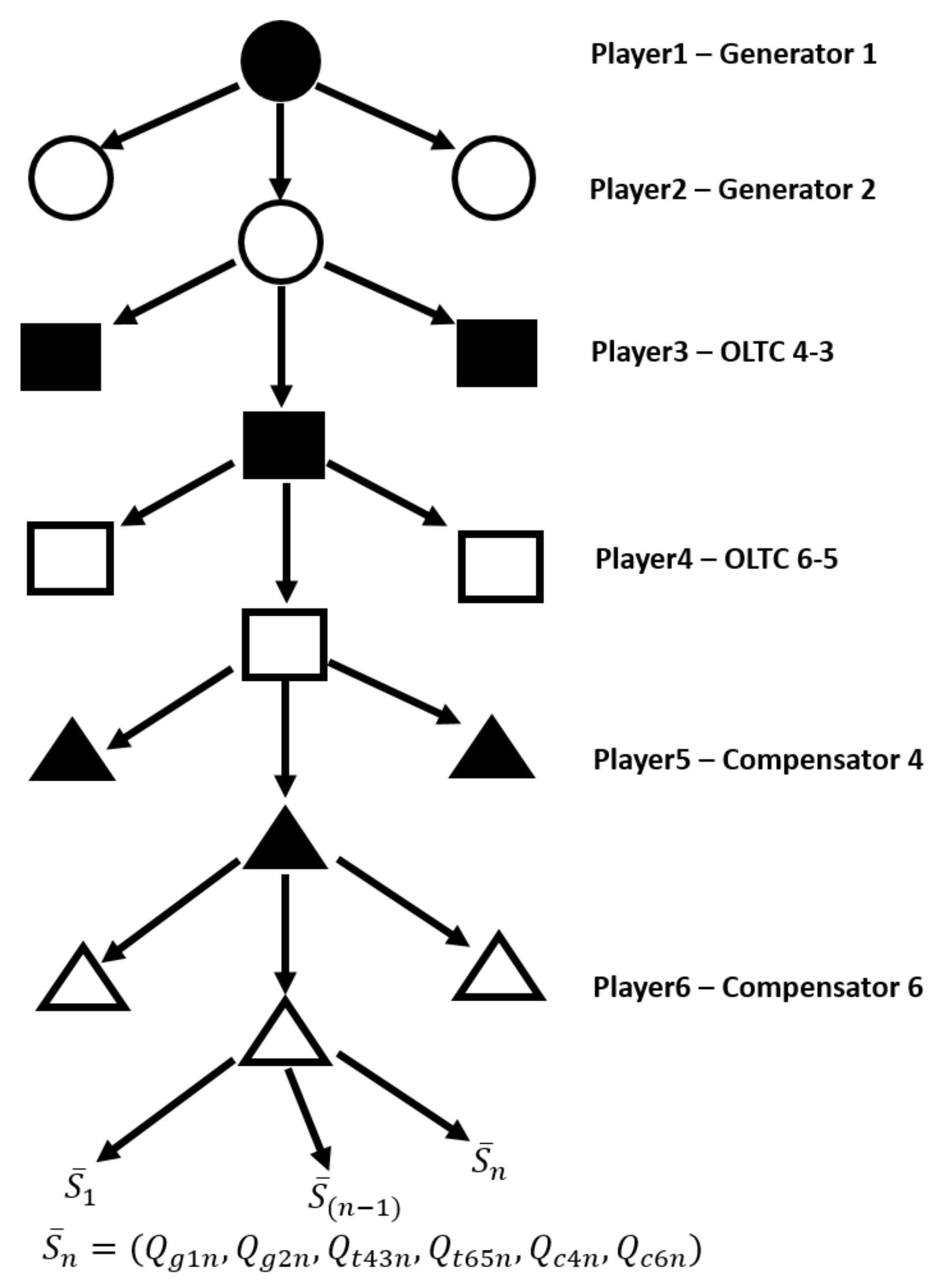
The resulting game tree, as applied to the IEEE 6-bus system, is illustrated in Figure 2, and it shows the hierarchical nature of interaction among the players. The symbols indicate the different components in the control flowchart: similar shapes indicate the same component type. For example, both generators are represented as circles, with the shaded one indicating generator 1 and the clear one generator 2.
4.10. Power Components’ Payoffs
Generators and compensators have reactive power injections and respectively, which represent payoffs for these power components. The reactive powers flowing across the OLTC-connected branches are considered to be their payoffs (i.e., ). is the payoff vector of players’ reactive power contributions for any nth chosen path. This is expressed as
where:
- : nth possible reactive power injections by generators 1 and 2.
- : nth possible reactive power flowing along OLTC branches connected to terminal buses 4 (6) and 3 (5).
- : nth possible reactive power injections by compensators at buses 4 and 6.
5. Game-Theoretic Equations and Algorithms
5.1. Formulated Game-Theoretic Equation
The backward induction solution is an important concept used to determine the credible Nash equilibrium of an extensive form game. It ensures that at every subgame, only the equilibrium path is followed, resulting in an overall Nash equilibrium for the whole game [14,16]. This process begins by observing the terminal nodes at the bottom of the tree. By stepping-up the tree, and following only the equilibrium paths, it ensures that a final solution which best satisfies the Nash equilibrium is reached. Applying the concept to this work, a game-theoretic equation that best represents the step-up process of the backward induction was formulated. The underlying goal is to find the optimal settings of power-system components, also known as players, that result in minimum reactive power contributions.
It must be noted that due to the breadth of the extensive form game, we will consider a single subgame for our discussion. We start at the bottom player node, i.e., player 6, where the set of terminal node-reactive power contributions corresponding to all n paths for one subgame is represented as:
For every subtree at this player node, we evaluate the reactive power contribution from player 6, i.e., , and choose the setting at the leaf node which minimizes this contribution to the system. The other leaf nodes with higher reactive power contributions are removed from the game before control is passed to player 5. The minimal reactive power contribution from player 6 is denoted by as shown below:
where is the surviving terminal node at the player node (player 5) for that subgame, and is the set of surviving terminal node payoffs at all subgames for the fifth player assignment.
Now we traverse upward through the tree and consider every subtree at that player node (player 5), for one subgame. The minimal reactive power contribution from player 5 is denoted by as shown below:
where is the surviving terminal node at the player node (player 4) for that subgame, and is the set of surviving terminal node payoffs at all subgames for the fourth player assignment.
This process continues until all surviving terminal nodes and subtrees are reached for the root node at player 1. For the last stage of backward induction, this results in:
where is the Nash equilibrium, and consists of the optimal reactive power contribution for all six players. The corresponding settings of the power system components are the equilibrium settings used to effect voltage and reactive power control in the system.
5.2. Formulated Game-Theoretic Algorithm
Two major stages are considered for this algorithm: data preparation and actual game play.
- (1)
- Data preparation: this stage was carried out prior to actual game play. After the determination of all the possible strategy profiles, the load voltage constraint was applied to filter out strategy profiles that did not satisfy the load voltage tolerance definition. This ensured that only valid profiles remained for game play activity. The data preparation process used to extract only the feasible profiles is shown in Algorithm 1.
- (2)
- Game play: this is the actual execution of backward induction beginning from the terminal node of the game tree. This stage is carried out after the data preparation stage, and this game play process is shown in Algorithm 2. By implementing steps (13)–(16), only profiles at every player node that ensure least reactive power contribution by that player are selected.
| Algorithm 1 Prior data preparation |
| Input:N-players ( with number of actions respectively; Define equality, inequality and load voltage constraints (10)–(11); Define load bus voltages i.e., ; Output: Vectors of load bus voltages and reactive power contributions |
| Invalidate combination settings with unacceptable voltages 1. For (Total combinations—) 2. Run power flow program; 3. Prune: If all load bus voltages satisfy voltage limits in (11) 4. Save: i, , component settings 5. Extract terminal nodes, Z←Reactive power payoff vectors 6. else Discard: i, , component settings 7. Proceed to i + 1 8. End |
| Algorithm 2 Reactive power game control (RPGC) |
| Input Vectors of load bus voltages and reactive power contributions Define mini = 9999 (Arbitrary large value) Output: Optimal component settings |
| # of players, N; Let players[P1,P2,P3,P4,P5,…PN] have [a,b,c,…]] possible actions For1:N do Fori = 1:a do 4: if Z←P1 then Goto (20) end if Forj = 1:b do if Z←P2 then Goto (20) 8: end if Fork = 1:c do if Z←P3 then Goto (20) end if 12: For l … … … if Z←P6 then 20: if reactive power cost ≤ mini then mini←reactive power cost SGE{ijklmn}←mini Assign SGE{ijklmn} as newly extracted terminal nodes, Z←P(N-1) 24: end if end if end for … … … End For Repeat algorithm until the root of the tree at player P1 is reached. SGE: Sub-game equilibrium |
6. Distributed Game Model
6.1. Power System Model
The New England 39-bus system was used to study the method of distributed control using the proposed game-theoretic algorithm. The one-line diagram and system data are presented in [21].
6.2. Decoupling
Due to the complex component interactions, it is not always possible to determine a global solution that satisfies all constraints imposed on a larger system. Hence, the proposed centralized game algorithm was extended with the objective of carrying out distributed control.
The steps that were carried out to implement distributed control are stated below:
- (1)
- Decoupling of the system into independent control areas.
- (2)
- Application of the GT algorithm to systematically control reactive power and voltage in each area. This will result in optimal control settings of the power system components in each control area.
- (3)
- A system convergence test using the optimal settings derived from step 2.
The concept of the boundary buses [3,22] was used to sectionalize the power system. This is a bus that interconnects two different areas and, through it, it is possible to model the influence of adjoining areas to which a desired area is connected.
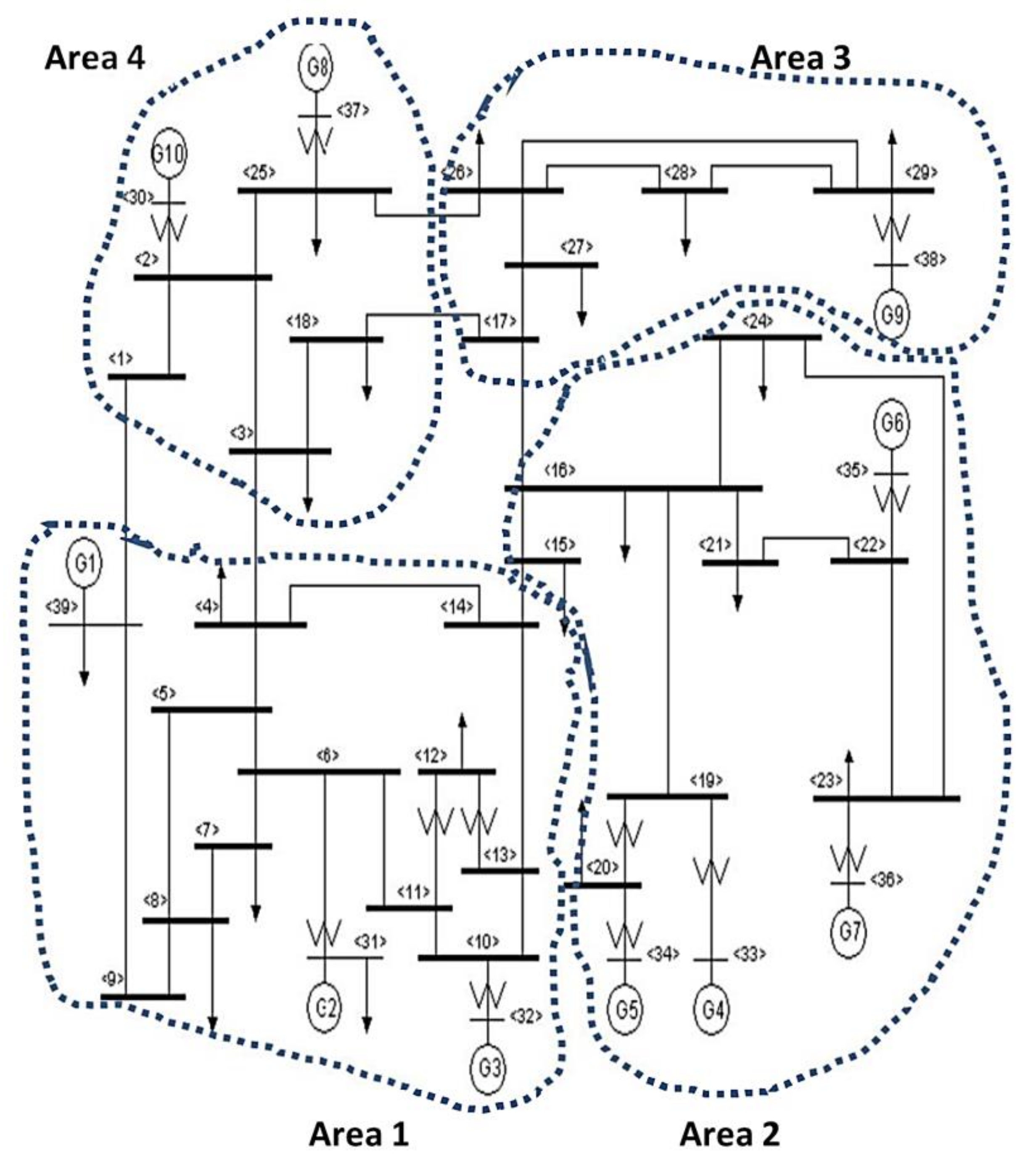
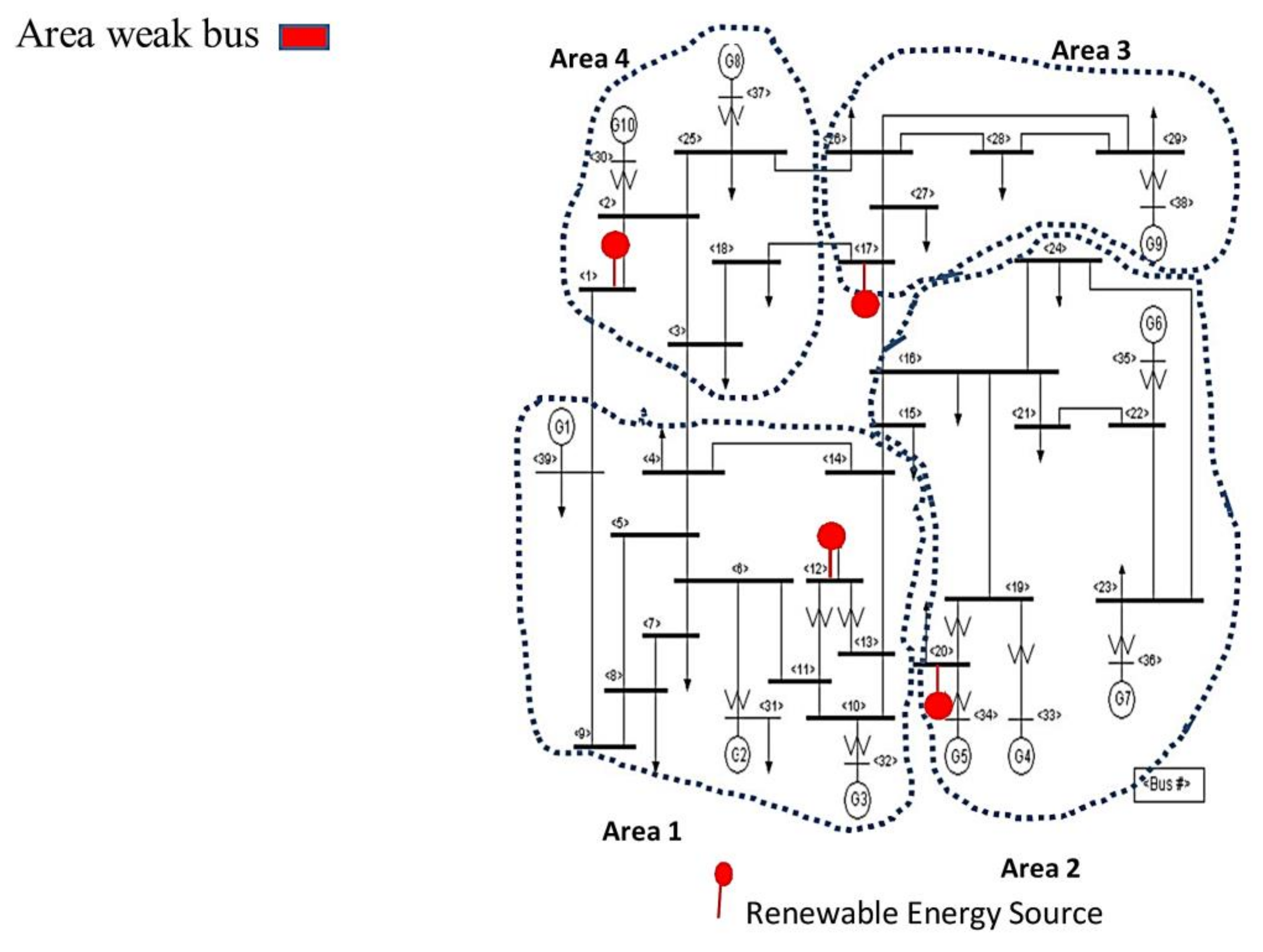
To decouple the system, a power flow for the New England 39-bus system was run for the base case. The 39-bus system was decoupled along three boundaries as in Zima and Ernst [3], with the addition of a fourth independent area. When solving load flow in each area, the largest rated generator is taken as the slack bus. In each of the four independent areas, the power flows into and out of each of the boundary buses were identified in order to determine the effective amount of reactive power connected to the bus [23]. The decoupled New England system has been illustrated in Figure 3. To determine the accuracy of the decoupling method used, the power-flow analysis is run for each of the four areas. To verify the decoupling method used, the voltage profile obtained from the superimposition of all four profiles from the independent areas is compared with the system-base voltage profile prior to decoupling.
6.3. Distributed Game-Theoretic Model
After successfully decoupling the system into individual control areas, the non-cooperative extensive form game formulated in Section 4 was applied in each of the areas. In the 39-bus system, only the generators were considered as players by maintaining all settings of the OLTCs to be constant. This was done in order to monitor the generators’ reactive power injections. The definitions of players, actions, payoffs and payoff vectors have been mentioned in the previous section. By executing the same processes in the formulated game equations and algorithms of Section 5, the optimal settings of system components in each area can be determined.
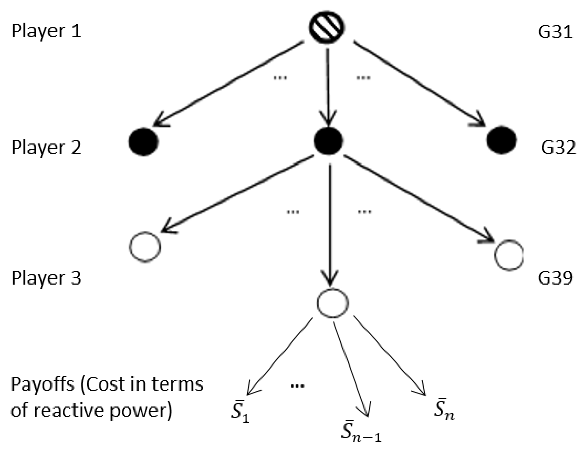
The game play for area 1 is illustrated in Figure 4. Similar game plays for the other areas are illustrated in [23]. Upon arriving at the optimal settings for each of the four independent areas, the power flow was run for the complete system using these new settings to determine the new system voltage profile.
7. Integration of Distributed, Renewable Energy Sources
System voltage profile could be improved by making use of distributed, local reactive sources. This could help accelerate the proposals of the European Union and the United States to achieve the renewable energy portfolio that has been targeted for 2020 and 2030, respectively [24].
In this paper, the placement and integration of renewable energies acting as reactive power sources is considered in order to improve system voltage compliance. Proper planning and adequate voltage analysis provides qualitative information on the state of system buses and will help operators take corrective actions to avoid voltage collapse [25,26]. Voltage stability analysis could either be static or dynamic [6,27]. While dynamic analysis is used to study system scenarios leading to voltage collapse and coordination of protection and controls, static analysis is used to study system snapshots at specified time frames [28]. Static voltage analysis is widely researched due to the slow variation of system voltage until a maximum loading condition is reached [29].
In this paper, the use of the voltage-reactive power (V-Q) sensitivity index [27,30], as a method for static analysis, is employed to identify vulnerable buses at which reactive support provided from renewable energy sources will be placed.
7.1. Voltage-Reactive Power (V-Q) Sensitivity
This method of analysis provides information on the variation of the magnitude of bus voltage due to a unit reactive power injection in that bus, and is also known as the reactive power sensitivity index [30]. By developing the linearized steady-state equations for the system [27,31] as shown in Equations (8) and (9), and solving using the Newton–Raphson technique, we obtain:
where ΔP, = Vectors of real and reactive bus power injection changes; Δδ, ΔV = vectors of bus voltage angle and magnitude changes; J = Jacobian matrix consisting of sub-matrices H, N, M and L; H, N = sensitivity matrix of bus real power to changes in voltage angle and magnitude, respectively; M, L = sensitivity matrix of bus reactive power to changes in voltage angle and magnitude, respectively.
For any n-bus system having number of load buses, number of generator buses and one slack bus,
The dimensions of the Jacobian and sub-matrices of Equation (17) are given as [32]:
Reactive and real powers are less sensitive to changes in voltage angle and voltage magnitude, respectively [27,30]. Hence, the sensitivity matrices N and M can be assumed to be negligible i.e.,
Further simplifications lead to:
The elements of the Jacobian matrix, L, are the approximate reactive power sensitivities with the diagonal elements considered as the sensitivities of each bus. By carrying out the partial differential of the reactive power at each bus (k) with respect to its bus voltage, these diagonal entries can be obtained as shown in the equation below:
is the summation of admittance between buses k and n;
7.2. Game-Theoretic Formulation and Approach
The separate load flows are run for each of the individual areas of the New England system as shown in Figure 3 using the optimal generator settings obtained from the distributed game control studied in Section 6. By making use of Equation (22), the resulting bus voltage magnitudes and angles are used as inputs to determine the sensitivities for each area bus. Comparing all the bus sensitivity indices in each of the four areas, the weakest bus in each area is identified, and renewable energy sources are integrated at these locations.
The proposed game-theoretic concept of Section 5 is applied to optimize all generator settings that will lead to the systematic control of reactive power and voltage. The buses at which renewable energy sources are connected are first considered to be generator buses in order to determine the amounts of reactive powers required to keep their load buses at specific voltage levels, followed by the determination of the optimal generator settings. Then, the renewable energy buses are changed to load buses at which reactive powers are being injected. Considering the optimal generator settings, the overall system load flow is run to observe the improved system voltage profile. Algorithm 3 illustrates the calculation of the sensitivity indices and game approach.
| Algorithm 3 Renewable energy integration at weak buses (REIWB) |
| @ each control area, 1: Solve power flow equations to obtain initial, at all buses 2: RPVS matrix, L is computed from with emphasis on the diagonal elements, To determine all entiries: Initialize empty array of RPVS_Diag_Entries For i = 1: Number of load buses For r = 1: Number of buses Initialize x = 0; If r = i, Sin else Sin() end end Update entries in RPVS_Diag_Entries end 3: Find weakest bus from min(RPVS_Diag_Entries) 4: Place renewable energy (acting as reactive power source) at PV bus to maintain voltage at 1.0 p.u. 5: Execute game algorithm to obtain optimal generator settings. 6: Solve power flow with optimal settings. 7: Determine reactive power injection by renewable energy source. Extract injected reactive power from renewable source in each area and update in overall system data. 8: Solve overall system power flow for new voltage profile; renewable energy buses are now PQ-buses. |
8. Simulation Results
Based on the formulated game algorithm, the MATLAB program (R2016b, MathWorks, Natick, MA, USA) was used to develop the game play and the Newton–Raphson technique required to run the required load flow analysis [28].
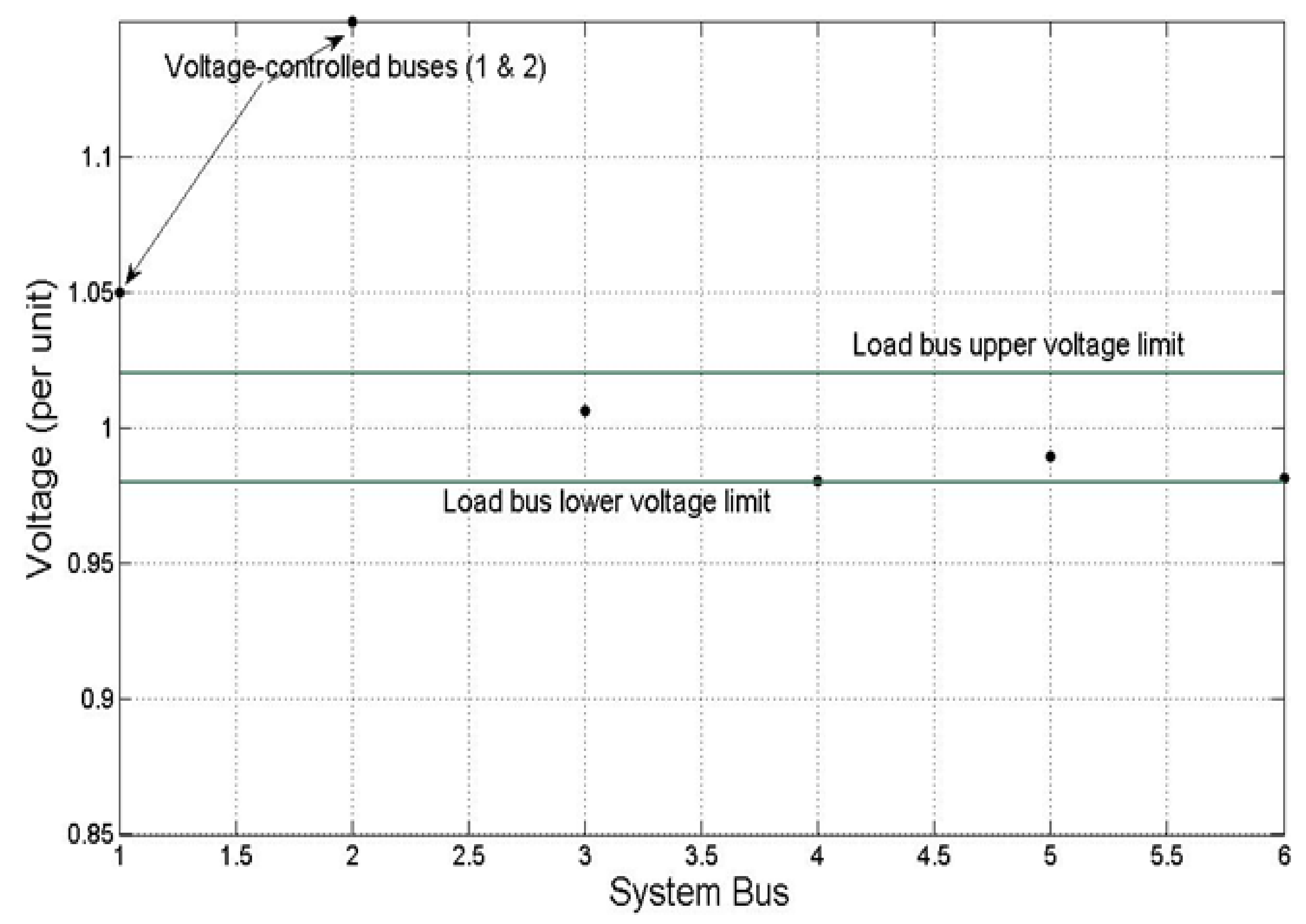
Table 1 and Table 2 and Figure 5 illustrate the equilibrium component settings, associated power flow and the resulting voltage profile after the game algorithm was applied systematically to control reactive power and voltage in the IEEE 6-bus system [20]. A total of 62,424 control combinations and possible solutions were obtained for the different settings of the voltage-control devices. Each of these settings constitute a strategy profile for the generators, tap-changing transformers, and compensators in the system, resulting in voltage control. The backward induction algorithm was then applied to feasible solutions i.e., only those combinations whose load voltages satisfied the required limits. The goal of the backward induction process is to determine the optimal profile by sequentially retaining only those profiles for which the reactive power contribution of a player is minimal at any subgame, while eliminating the others.
As the first player in the backward induction algorithm, compensator 6 (player 6) attempts to maximize its payoff at each subgame. It achieves this by choosing the setting at the leaf node which minimizes its reactive power contribution to the system. The other leaf nodes with higher reactive power requirements are removed from the game before control is passed to compensator 4 (player 5). Similarly, player 5 maximizes its payoff at each subgame. At the final decision node, the two remaining strategy profiles are shown in Table 1.
Applying the backward induction algorithm for reactive power control i.e., Algorithm 2, several strategy profiles are eliminated by players 2 to 5 (in reversed order) in a bid to minimize their individual reactive power contributions. The two surviving profiles in the game are indexed 34,596 and 45,504, from which the choice of the optimal profile is made by player 1 (generator 1). The voltage settings of Generator 1, 1.05 or 1.1 p.u., from either of the two strategy profiles 34,596 and 45,504 satisfy the voltage requirements at all load buses. However, as seen from Table 2, in order to maximize its payoff, generator 1 injects a lower reactive power into the system (20.93 MVAr), thus choosing a voltage set point of 1.05 p.u. instead of 1.1 p.u. Generator 1 utilizes a minimal amount of reactive power to provide satisfactory voltage levels at all buses, while still ensuring a higher reactive power in its reserve. Strategy profile 34,596 forms the Nash equilibrium strategy for the game.
It can be observed that system voltage profile was brought within the pre-defined, accepted voltage tolerance limits. At the same time, the reactive power contribution of each component was minimized based on the order of action.
The game-theoretic control was now adapted for distributed control in the 39-bus system. A load flow was run for the base case. Based on the power flows into and out of the boundary bus, the influence of adjoining areas was modeled as an effective power flow into or out of the boundary bus. This was carried out for all four control areas, and load flow analysis for each of these areas resulted in the same voltage profile as earlier obtained from the base case. System data for each area was modified to reflect the decoupled system [23].
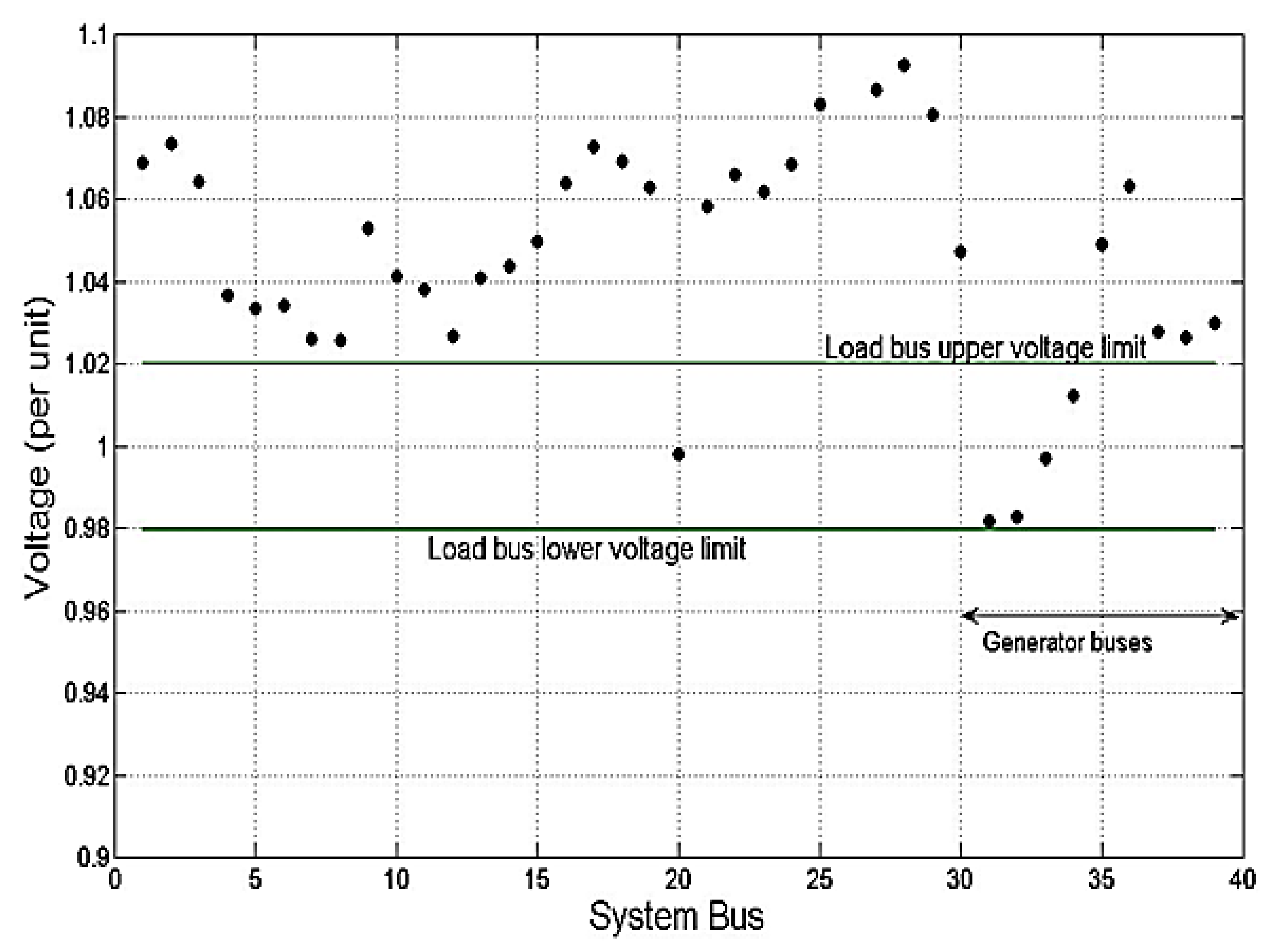
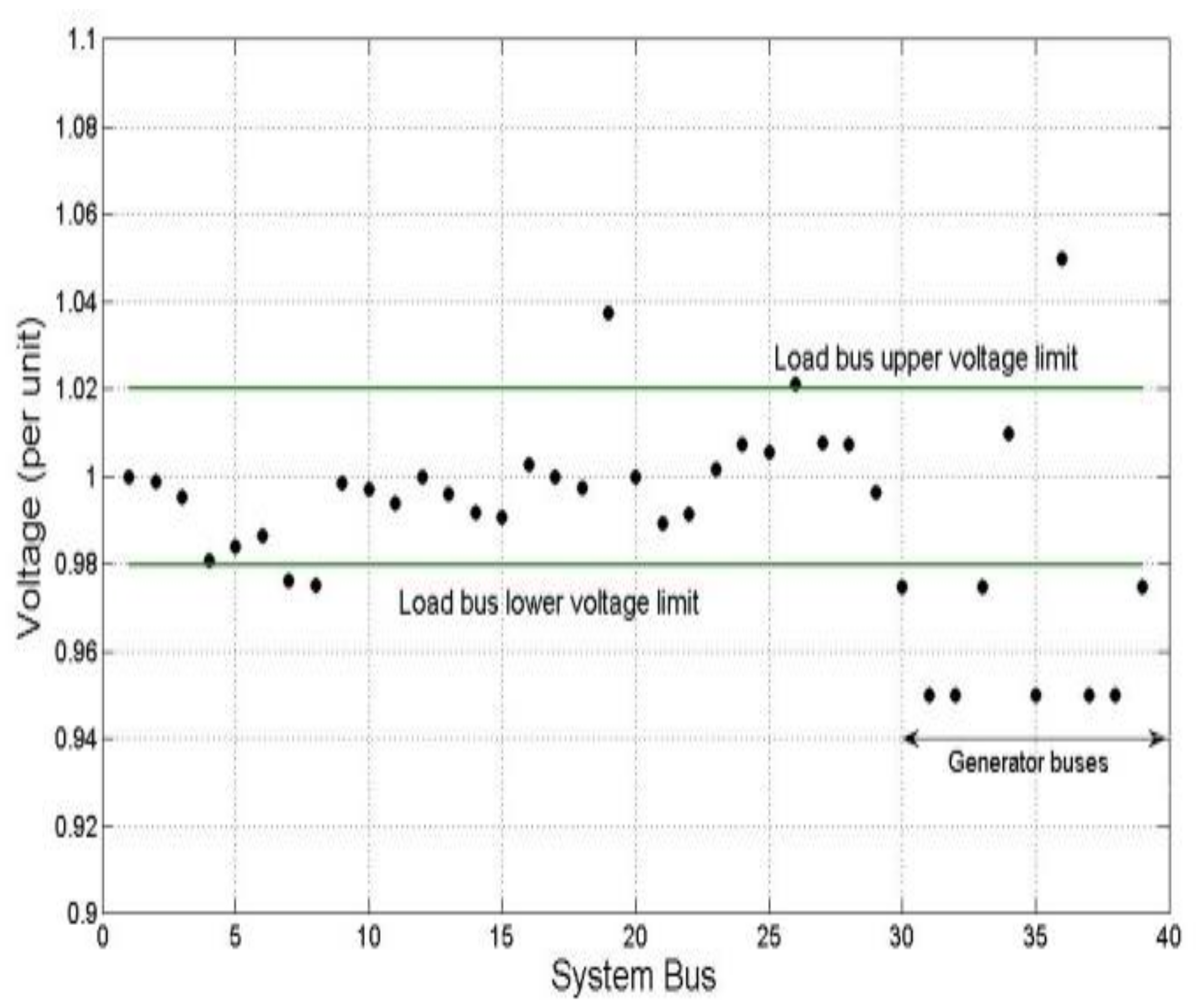
The voltage profile for the base case is illustrated in Figure 6 and this shows voltage deviations at a majority of the load buses (97%) in the system based on the 0.98–1.02 p.u. tolerance. Also, the amount of reactive power lost in the system is −1423.997 VAr. This implies excessive reactive power generation by the system largely due to overvoltage.
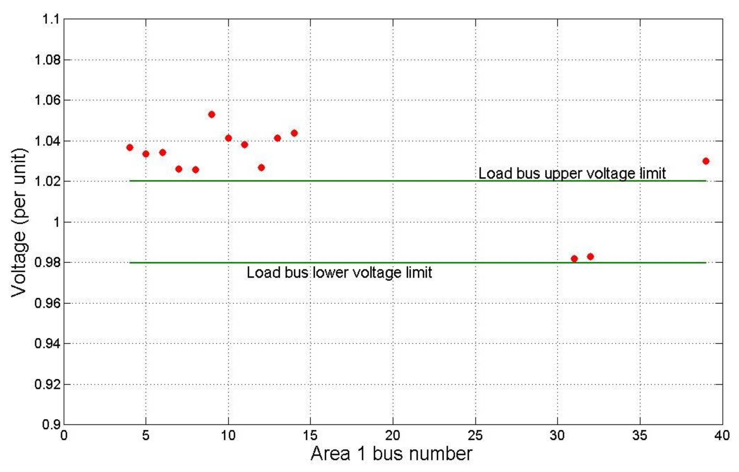
Figure 7 illustrates the bus voltage profile for a given decoupled area 1. It is observed that the resulting area bus voltage profile after decoupling is similar to that of the unified, base case. For all other areas, the bus voltage profile remained the same. This confirmed the accuracy of the decoupling method used.
The players were identified in each area, considering only generators; all OLTC tap settings remained constant, hence were not participants in the game play. The actions considered for the generators were the same as those proposed in the centralized control i.e., the fixed steps between the AVR control ranges.
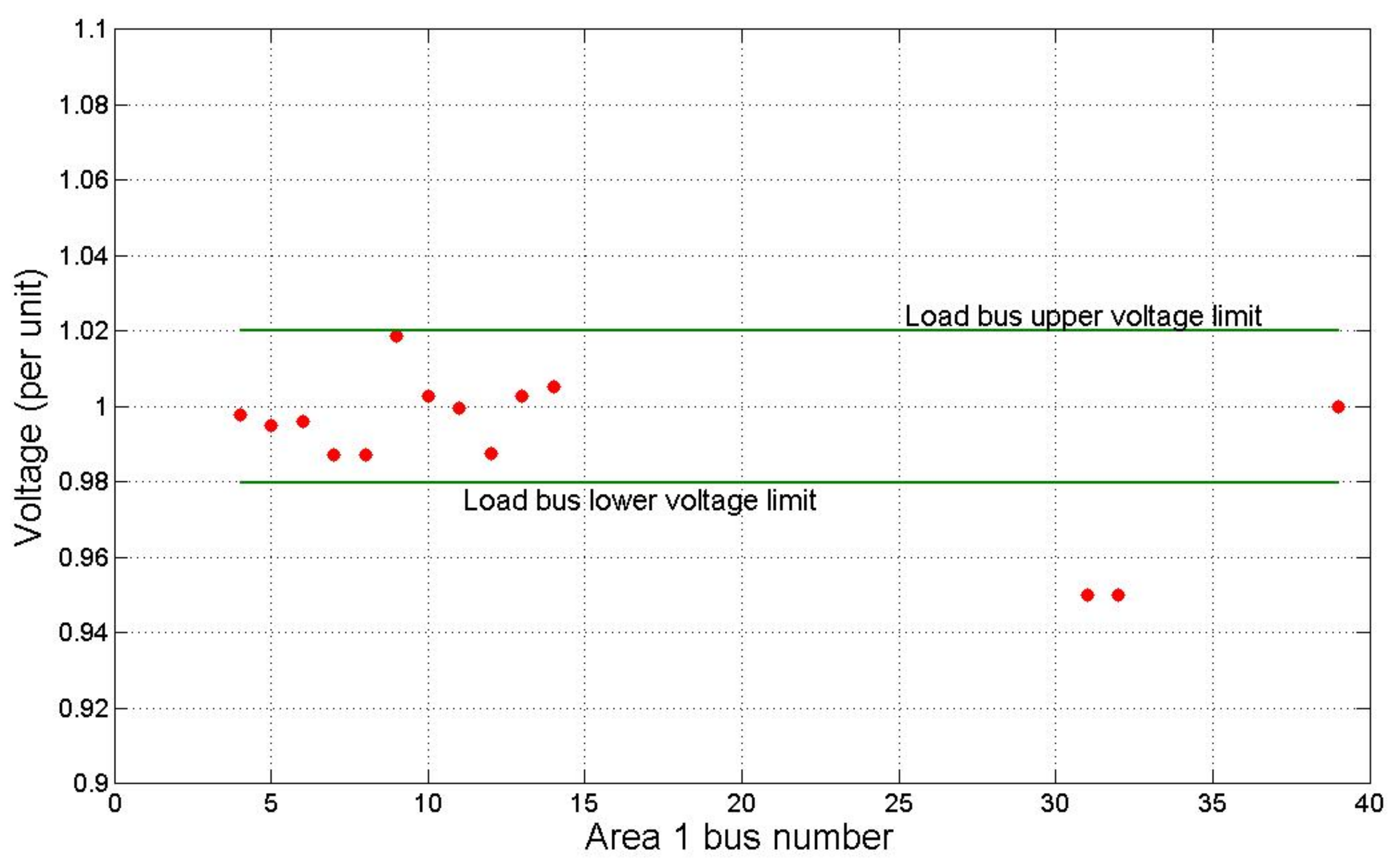
Upon application of the game-control algorithm in each area, it resulted in a set of optimal control settings for each player in that area. The graph in Figure 8 displays the voltage profile, based on the optimal generator settings, for an independent control area 1 after the application of the game-control algorithm.
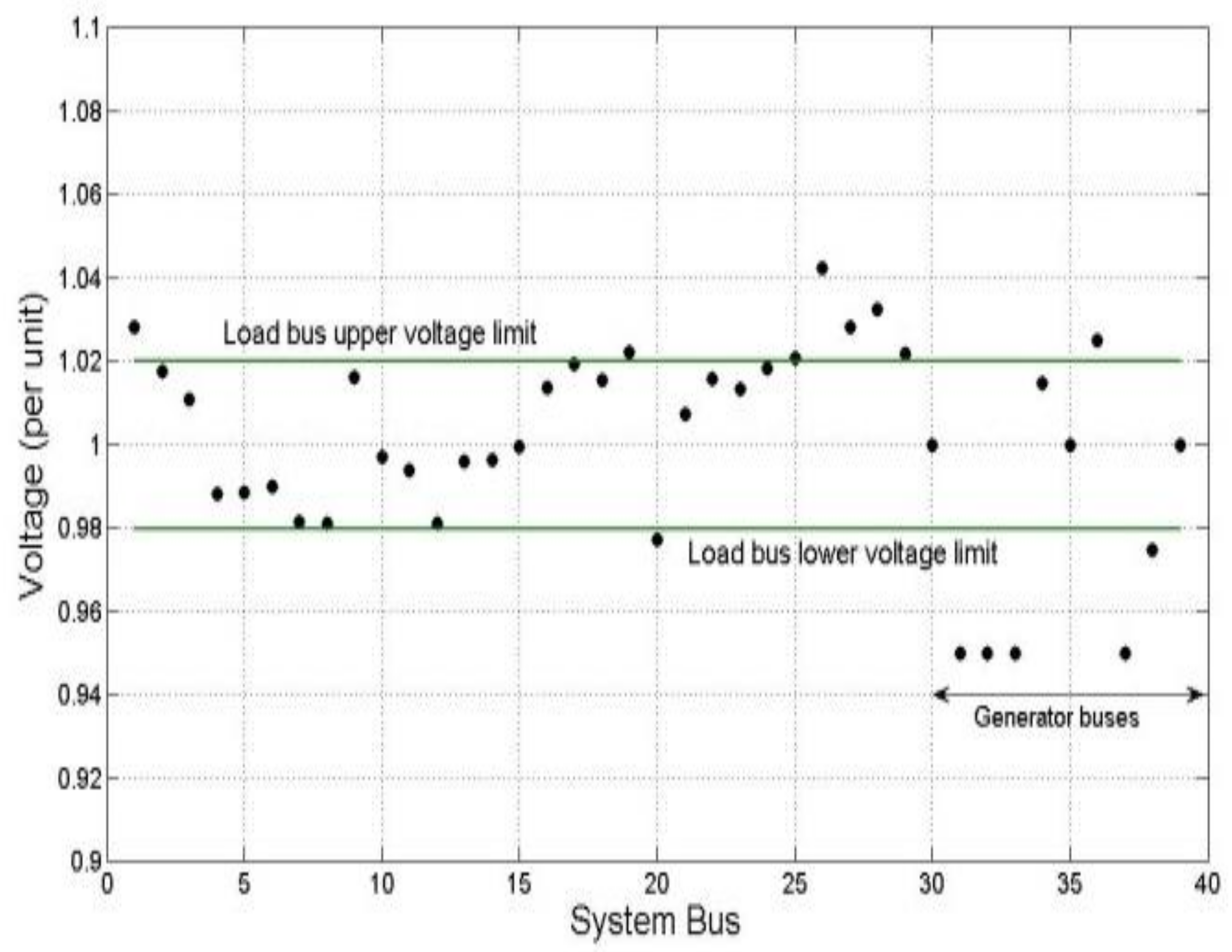
The post-game voltage profiles for the other areas are illustrated in [23]. An overall system convergence test was run based on the optimal generator settings derived from each area. These optimal generator settings for all four areas are shown in Table 3, and the resulting convergence voltage profile for the system is illustrated in Figure 9. It can be observed that 75% of the load buses satisfied the voltage tolerance earlier specified. Also, the optimal settings for most of the generators showed that their AVR settings lie close to the lower limit of operation.
From this result, it can be inferred that more capacity for generator AVR control exists for future contingencies. Finally, the reactive power lost from the system was reduced to −1113.466 VAr. Even though this meant reactive power generation by the system, it can be observed that the amount being generated is less than that generated in the base case of the system.
Table 4 shows the sensitivity indices calculated for all buses located in their respective areas. Comparing the indices in each area, it can be observed that bus numbers 12, 20, 17 and 1 make up the weakest area buses in the system. These buses were identified as the best locations for the placement of the supporting renewable energy sources. Figure 10 illustrates the 39-bus system with the renewable energy sources now integrated. The game-theoretic control was applied to each area in order to determine the required amounts of reactive power injections needed to maintain all area renewable energy buses at 1.0 p.u. These buses were considered as generator-types which regulate bus voltages.
Table 5 shows the reactive power support required at each of these four buses. A minimal reactive power of 33 MVAr is required from bus 1 with a maximum of 178 MVAr required at bus 20. The new optimal generator settings, considering the renewable energy sources, are presented in Table 6. Based on these generator settings and the reactive powers required from the supporting renewable energy buses, an overall system load flow was run. Figure 11 shows the resulting system voltage profile.
It was observed that 86% of the load buses complied with the voltage limits. This was an improvement on the 75% compliance earlier obtained from the game-controlled system without renewable-energy integration.
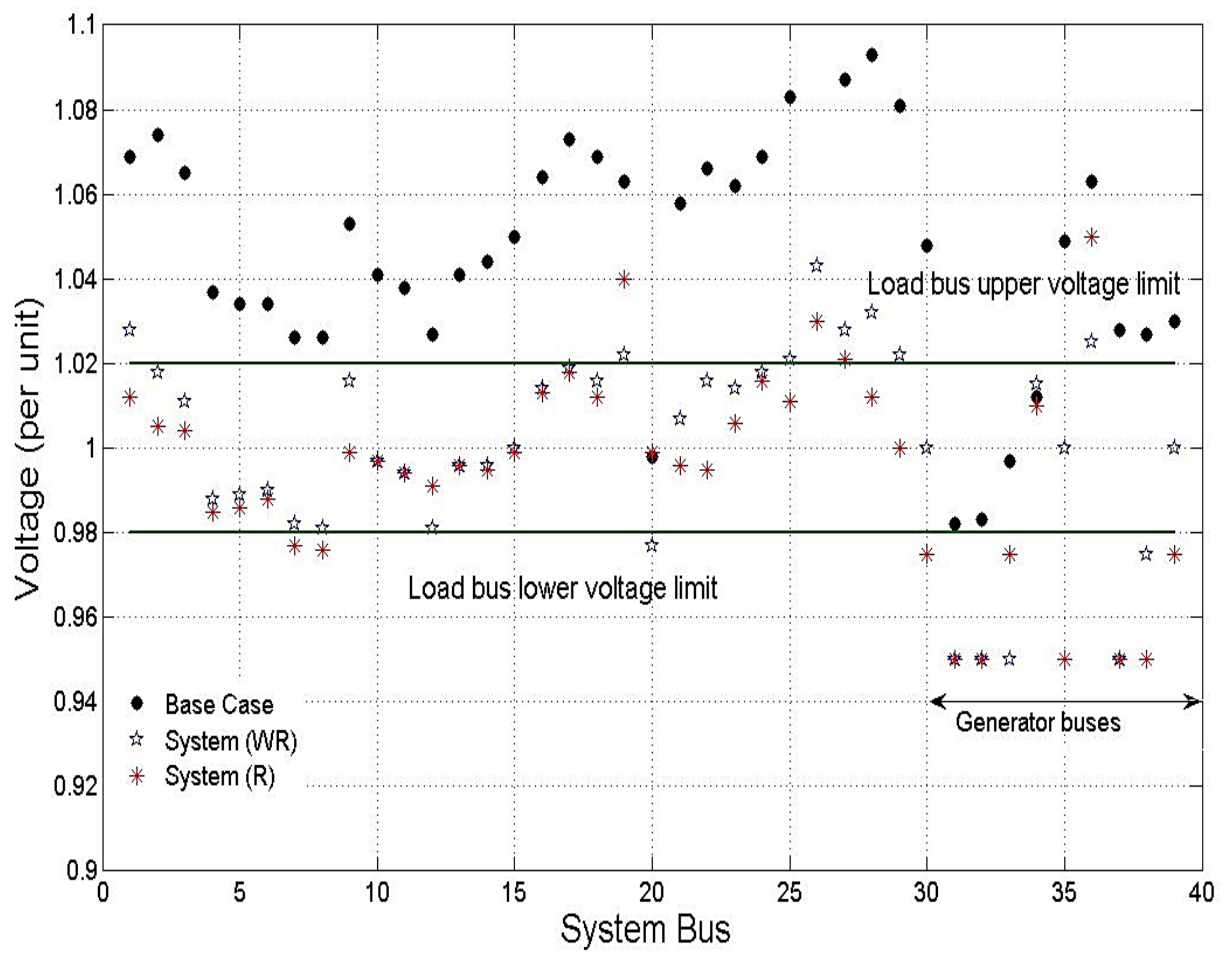
Figure 12 presents the voltage profile comparisons for all three cases (base, distributed alone, and distributed with renewable energy integration). In Table 7, both optimal generator settings for the system considering renewable-energy integration and without renewable energies (WR) are compared. It can be observed that more generator AVR settings for the R-case lie closer to the lower operating limits. This implies a lesser burden on generators for reactive power since the renewable-energy sources largely act as reactive power compensators. The effective system generators’ reactive power contributions is a total of 51 MVAr, a drastic decrease from 295 MVAr initially supplied when no renewable-energy source was used. This result is a further improvement on generator reserve reactive power to handle future contingencies. The use of generators, as quick and temporary sources of reactive power [1], to keep the system stable, is further enhanced.
9. Conclusions
In this work, a novel application of the extensive form game theoretic model was carried out in a power grid in order to control reactive power flow and voltage systematically. A centralized method for control was developed and further translated to a method for distributed control.
As shown in the results for the centralized control, the ability to filter out all intolerable voltage profile results before systematically controlling reactive power based on any defined hierarchical interaction of components is essential to arrive at equilibrium component control settings. By ensuring that components contribute minimally to reactive power when controlling system voltage, reserved capacity for future contingencies is increased. Also, the amount of power flow in the line is reduced.
Scaling up this method to a larger system, a 39-bus network was decoupled into four different areas using a boundary bus technique. The proposed game-control algorithm was applied at each of the areas to determine optimal generator settings. The overall system load voltage compliance was increased from 3% to 75%. Furthermore, the reactive power-voltage sensitivity method was used to identify the weakest buses at which renewable energies (acting as reactive power sources) were integrated. With a new set of optimal generator settings and renewable energies (reactive sources), an improved 85% load-voltage compliance was observed.
As shown in this work, game theory can be used as an effective tool for managing power-system operations. The use of the proposed game-theoretic technique adapts well to reactive-power conservation in the control of system voltage and the determination of optimal settings of power-system components.
Acknowledgments
This work was supported in part by the Engineering Research Center Program of the National Science Foundation and the Department of Energy under NSF Award Number EEC-1041877 and the CURENT Industry Partnership Program.
Author Contributions
Ikponmwosa Idehen, Shiny Abraham, and Gregory V. Murphy conceived the idea; Ikponmwosa Idehen and Shiny Abraham designed the experiments; Ikponmwosa Idehen performed the experiments and analyzed the data; Shiny Abraham and Gregory V. Murphy contributed analysis tools; Ikponmwosa Idehen wrote the paper, and Shiny Abraham reviewed and edited the paper.
Conflicts of Interest
The authors declare no conflict of interest.
Nomenclature
| nth possible reactive power injection by generator or compensator component labeled | |
| nth possible reactive power flow along transformer branch and | |
| Voltage at generator bus | |
| Reactive power injection at generator bus | |
| Voltage at bus | |
| Complex power flowing from bus to | |
| Bus admittance entry between buses and | |
| Transformer branch reactive power from to | |
| Transformer tap settings between buses and | |
| nth payoff vector comprising reactive power contributions for all players for any | |
| For any subgame and ith player assignment, the set of all payoffs located at the leaf or terminal nodes |
References
- Phulpin, Y.; Begovic, M.; Ernst, D. Coordination of voltage control in a power system operated by multiple transmission utilities. In Proceedings of the 2010 IREP Symposium Bulk Power System Dynamics and Control—VIII (IREP), Rio de Janeiro, Brazil, 1–6 August 2010; pp. 1–8. [Google Scholar]
- Zhang, A.; Li, H.; Liu, F.; Yang, H. A coordinated voltage/reactive power control method for multi-TSO power systems. Int. J. Electr. Power Energy Syst. 2012, 43, 20–28. [Google Scholar] [CrossRef]
- Zima, M.; Ernst, D. On multi-area control in electric power systems. In Proceedings of the 15th Power System Computation Conference (PSCC), Liège, Belgium, 22–26 August 2005; pp. 22–26. [Google Scholar]
- Mousavi, O.A.; Cherkaoui, R. On the inter-area optimal voltage and reactive power control. Int. J. Electr. Power Energy Syst. 2013, 52, 1–13. [Google Scholar] [CrossRef]
- Dong, F.; Howdhury, B.H.; Crow, M.L.; Acar, L. Power Reserve Management. IEEE Trans. Power Syst. 2005, 20, 338–345. [Google Scholar] [CrossRef]
- Kundur, P. Power Systems Stability and Control; Mc-Graw Hill: New York, NY, USA, 1994; pp. 967–996. [Google Scholar]
- Schlueter, R.A. A voltage stability security assessment method. IEEE Trans. Power Syst. 1998, 13, 1423–1438. [Google Scholar] [CrossRef]
- Pradeep, H.; Venugopalan, N. A study of voltage collapse detection for power systems. Int. J. Emerg. Technol. Adv. Eng. 2013, 3, 325–331. [Google Scholar]
- Mantawy, A.H.; Al-Ghamdi, M.S. A new reactive power optimization algorithm. In Proceedings of the 2003 IEEE Bologna Power Tech Conference Proceedings, Bologna, Italy, 23–26 June 2003; pp. 470–475. [Google Scholar]
- Sharma, N.K.; Babu, D.S. Application of particle swarm optimization technique for reactive power optimization. In Proceedings of the IEEE-International Conference on Advances in Engineering, Science And Management (ICAESM-2012), Tamil Nadu, India, 30–31 March 2012; pp. 88–93. [Google Scholar]
- Vlachogiannis, J.G.; Lee, K.Y. A comparative study on particle swarm optimization for optimal steady-state performance of power systems. IEEE Trans. Power Syst. 2006, 21, 1718–1728. [Google Scholar] [CrossRef]
- Bakare, G.A.; Venayagamoorthy, G.K.; Member, S.; Aliyu, U.O. Reactive power and voltage control of the Nigerian grid system using micro-genetic algorithm. Power Eng. Soc. Meet. 2005, 2, 1916–1922. [Google Scholar]
- Yoshida, H.; Kawata, K. A particle swarm optimization for reactive power and voltage control. IEEE Trans. Power Syst. 2001, 15, 1232–1239. [Google Scholar] [CrossRef]
- Leyton-Brown, K.; Shoham, Y. Essentials of Game Theory: A Concise Multidisciplinary Introduction; Morgan and Claypool: San Rafael, CA, USA, 2008; pp. 3–40. [Google Scholar]
- Osborne, M.J.; Rubinstein, A. A Course in Game Theory; MIT Press: Cambridge, UK, 2011; pp. 1–19. [Google Scholar]
- Rasmusen, E. Games and Information: An Introduction to Game Theory, 3rd ed.; Blackwell: Oxford, UK, 2001; pp. 15–60. [Google Scholar]
- Holler, M.J. Classical, Modern and New Game Theory; Hamburg, Germany, 2001. Available online: https://law.yale.edu/system/files/documents/pdf/holler.pdf (accessed on 18 July 2014).
- Kuhn, H.W.; Harsanyu, J.C.; Selten, R.; Weibull, J.W.; van Damme, E.; Nash, J.F., Jr.; Hammerstein, P. The work of John F. Nash Jr. in game theory: Nobel Seminar. Duke Math. J. 1995, 81, 1–29. [Google Scholar] [CrossRef]
- Momoh, J.A. Electric Power System Applications of Optimization; CRC Press: Boca Raton, FL, USA, 2000. [Google Scholar]
- Idehen, I.; Abraham, S.; Murphy, G.V. Reactive power and voltage control in a power grid: A game-theoretic approach. In Proceedings of the 2018 IEEE Texas Power and Energy Conference (TPEC), College Station, TX, USA, 8–9 February 2018; pp. 1–6. [Google Scholar]
- The IEEE 10 Generator 39 Bus System. Available online: http://sys.elec.kitami-it.ac.jp/ueda/demo/WebPF/39-New-England (accessed on 11 January 2014).
- Granada, M.; Rider, M.J.; Mantovani, J.R.S.; Shahidehpour, M. A decentralized approach for optimal reactive power dispatch using a Lagrangian decomposition method. Electr. Power Syst. Res. 2012, 89, 148–156. [Google Scholar] [CrossRef]
- Idehen, I. A Method for Distributed Control of Reactive POWER and Voltage in a Power Grid: A Game-Theoretic Approach. Master’s Thesis, Tuskegee University, Tuskegee, Alabama, 2014, unpublished. [Google Scholar]
- Samad, T.; Annaswamy, A.M. Control for Renewable Energy and Smart Grids. Impact of Control Technology. 2011. Available online: www.ieeecss.org (accessed on 18 July 2014).
- Chowdhury, B.H.; Taylor, C.W. Voltage Stability Analysis: V-Q Power Flow Simulation Versus Dynamic Simulation. IEEE Trans. Power Syst. 2000, 15, 1354–1359. [Google Scholar] [CrossRef]
- Sinha, A.K.; Hazarika, D. A comparative study of voltage stability indices in a power system. Int. J. Electr. Power Energy Syst. 2000, 22, 589–596. [Google Scholar] [CrossRef]
- Roy, P.; Bera, P.; Halder, S.; Das, P.K. Reactive power sensitivity index based voltage stability analysis to a real system (400 kV system of WBSEB). Int. J. Electron. Commun. Technol. 2013, 7109, 167–169. [Google Scholar]
- Saadat, H. Power Systems Analysis (MATLAB Codes), 3rd ed.; PSA Publishing: London, UK, 2010; pp. 271–274. [Google Scholar]
- Anand, U.P.; Dharmeshkumar, P. Voltage stability assessement using continuation power flow. Int. J. Adv. Res. Electr. Electron. Instrum. Eng. 2013, 2, 4013–4022. [Google Scholar]
- Santos, J.R.; Ramos, E.R. Voltage sensitivity based technique for optimal placement of switched capacitors. In Proceedings of the 15th Power Systems Computation Conference, Liège, Belgium, 22–26 August 2005; pp. 22–26. [Google Scholar]
- Moradzadeh, M.; Boel, R. Voltage coordination in multi-area power systems via distributed model predictive control. IEEE Trans. Power Syst. 2013, 28, 513–521. [Google Scholar] [CrossRef]
- Ghosh, A. Load Flow by Newton-Raphson Method. Power Systems Analysis (Web). Available online: http://nptel.ac.in/courses/Webcourse-contents/IIT-KANPUR/power-system/chapter_4/4_10.html (accessed on 18 July 2014).
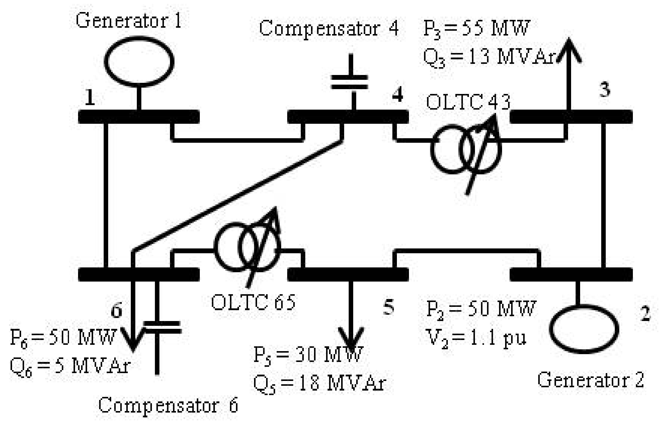
Figure 1.
IEEE 6-bus system.

Figure 2.
Non-cooperative extensive form game model (with perfect information).

Figure 3.
The decoupled New England 39-bus system.

Figure 4.
Extensive form game model for Area 1.

Figure 5.
The 6-bus equilibrium voltage profile after game.

Figure 6.
The base voltage profile for the 39-bus system.

Figure 7.
Distributed control: base voltage for decoupled area 1.

Figure 8.
Distributed control: post-game theoretic (GT) Area 1 voltage profile.

Figure 9.
The 39-bus system voltage profile after game-control algorithm was applied.

Figure 10.
The New England 39-bus system with renewable-energy sources.

Figure 11.
System voltage profile with renewable-energy sources after game control.

Figure 12.
System voltage profiles for the base case, post-game without renewable (WR) and with renewable (R) sources.
Figure 12.
System voltage profiles for the base case, post-game without renewable (WR) and with renewable (R) sources.


Table 1.
Equilibrium component settings.
| Strategy Profiles | 34,596 | 45,504 |
|---|---|---|
| Voltage setting gen 2 (p.u.) | 1.05 | 1.10 |
| Tap setting of OLTC 4-3 | 0.9625 | 0.975 |
| Tap setting of OLTC 6-5 | 1.0000 | 0.9625 |
| Vars from compensator 4 (p.u.) | 5.0 | 5.0 |
| Vars from compensator 6 (p.u.) | 5.5 | 5.5 |
| Voltage setting gen 1 (p.u.) | 1.05 | 1.10 |
| Vars from gen 1 (MVAr) | 20.93 | 41.91 |
Table 2.
Power flow results for equilibrium strategy.
| Bus | Volt (p.u.) | Angle (deg) | Pg (MW) | Qg (MVAr) | Qsh (p.u.) |
|---|---|---|---|---|---|
| 1 | 1.050 | 0 | 94.736 | 20.929 | 0 |
| 2 | 1.150 | −9.082 | 50.000 | 32.477 | 0 |
| 3 | 1.006 | −13.369 | 0 | 0 | 0 |
| 4 | 0.980 | −10.161 | 0 | 0 | 5.0 |
| 5 | 0.989 | −11.418 | 0 | 0 | 0 |
| 6 | 0.982 | −11.884 | 0 | 0 | 5.5 |
Table 3.
Equilibrium generator settings for all areas.
| Area | Generator Bus | Base Voltage (p.u.) | Optimal Voltage (p.u.) |
|---|---|---|---|
| 4 | 30 | 1.048 | 1.000 |
| 1 | 31 | 0.982 | 0.950 |
| 1 | 32 | 0.983 | 0.950 |
| 2 | 33 | 0.997 | 0.950 |
| 2 | 34 | 1.012 | 1.015 |
| 2 | 35 | 1.049 | 1.000 |
| 2 | 36 | 1.063 | 1.025 |
| 4 | 37 | 1.028 | 0.950 |
| 3 | 38 | 1.027 | 0.975 |
| 1 | 39 | 1.030 | 1.000 |
Table 4.
V-Q sensitivity indices for all area buses.
| Area | Load Bus | Sensitivity Index |
|---|---|---|
| 1 | 4 | 307.4 |
| 5 | 805 | |
| 6 | 1076.6 | |
| 7 | 515.7 | |
| 8 | 497 | |
| 9 | 70 | |
| 10 | 682.5 | |
| 11 | 603.5 | |
| 12 | 44.3 | |
| 13 | 515.4 | |
| 14 | 391.5 | |
| 2 | 15 | 224.51 |
| 16 | 660.36 | |
| 19 | 242.4 | |
| 20 | 188.85 | |
| 21 | 345.4 | |
| 22 | 347.01 | |
| 23 | 235.75 | |
| 24 | 208.65 | |
| 3 | 17 | 55.68 |
| 26 | 238.58 | |
| 27 | 234.28 | |
| 28 | 260.16 | |
| 29 | 333.33 | |
| 4 | 1 | 70.92 |
| 2 | 623.8 | |
| 3 | 278.73 | |
| 18 | 77.97 | |
| 25 | 168.53 |
Table 5.
Sensitivity indices for all buses’ reactive power injections from renewable energy sources.
Table 5.
Sensitivity indices for all buses’ reactive power injections from renewable energy sources.
| Area | Weak Bus | Injected Reactive Power (VAr) |
|---|---|---|
| 1 | 12 | 44.621 |
| 2 | 20 | 178.041 |
| 3 | 17 | 53.581 |
| 4 | 1 | 32.678 |
Table 6.
Equilibrium generator settings for all areas with renewable energy.
| Area | Weak Bus | Injected Reactive Power (VAr) |
|---|---|---|
| 1 | 12 | 44.621 |
| 2 | 20 | 178.041 |
| 3 | 17 | 53.581 |
| 4 | 1 | 32.678 |
Table 7.
Comparison of automatic voltage regulator (AVR) settings for all three cases.
| Bus | Base | Post-Game (WR) | Post-Game (R) |
|---|---|---|---|
| 30 | 1.048 | 1.000 | 0.975 |
| 31 | 0.982 | 0.950 | 0.950 |
| 32 | 0.983 | 0.950 | 0.950 |
| 33 | 0.997 | 0.950 | 0.975 |
| 34 | 1.012 | 1.015 | 1.010 |
| 35 | 1.049 | 1.000 | 0.950 |
| 36 | 1.063 | 1.025 | 1.050 |
| 37 | 1.028 | 0.950 | 0.950 |
| 38 | 1.027 | 0.975 | 0.950 |
| 39 | 1.030 | 1.000 | 0.975 |
© 2018 by the authors. Licensee MDPI, Basel, Switzerland. This article is an open access article distributed under the terms and conditions of the Creative Commons Attribution (CC BY) license (http://creativecommons.org/licenses/by/4.0/).
Share and Cite
MDPI and ACS Style
Idehen, I.; Abraham, S.; Murphy, G.V. A Method for Distributed Control of Reactive Power and Voltage in a Power Grid: A Game-Theoretic Approach. Energies 2018, 11, 962. https://doi.org/10.3390/en11040962
AMA Style
Idehen I, Abraham S, Murphy GV. A Method for Distributed Control of Reactive Power and Voltage in a Power Grid: A Game-Theoretic Approach. Energies. 2018; 11(4):962. https://doi.org/10.3390/en11040962
Chicago/Turabian StyleIdehen, Ikponmwosa, Shiny Abraham, and Gregory V. Murphy. 2018. "A Method for Distributed Control of Reactive Power and Voltage in a Power Grid: A Game-Theoretic Approach" Energies 11, no. 4: 962. https://doi.org/10.3390/en11040962
Note that from the first issue of 2016, this journal uses article numbers instead of page numbers. See further details here.