A Heuristic T-S Fuzzy Model for the Pumped-Storage Generator-Motor Using Variable-Length Tree-Seed Algorithm-Based Competitive Agglomeration

Abstract

With the fast development of artificial intelligence techniques, data-driven modeling approaches are becoming hotspots in both academic research and engineering practice. This paper proposes a novel data-driven T-S fuzzy model to precisely describe the complicated dynamic behaviors of pumped storage generator motor (PSGM). In premise fuzzy partition of the proposed T-S fuzzy model, a novel variable-length tree-seed algorithm based competitive agglomeration (VTSA-CA) algorithm is presented to determine the optimal number of clusters automatically and improve the fuzzy clustering performances. Besides, in order to promote modeling accuracy of PSGM, the input and output formats in the T-S fuzzy model are selected by an economical parameter controlled auto-regressive (CAR) model derived from a high-order transfer function of PSGM considering the distributed components in the water diversion system of the power plant. The effectiveness and superiority of the T-S fuzzy model for PSGM under different working conditions are validated by performing comparative studies with both practical data and the conventional mechanistic model.

1. Introduction

With the ever-increasing interconnection of intermittent renewable energy in modern power systems, the pumped-storage power plant (PSPP) plays a significant role in maintaining the balance of power supply and demand due to its flexible operations in both generation and pumping directions [1]. As the core part of PSPP, pumped-storage generator-motor (PSGM) is known as a hydraulic-mechanical-electrical coupling system with complicated nonlinear dynamic characteristics, which makes it a tough and challenging work to precisely modelling its dynamic behaviors under different operating conditions.

In traditional system modeling approaches of PSGM, the complete characteristic curves [2,3,4,5] and the method of characteristics [6,7,8,9] are utilized together to precisely simulate the hydraulic nonlinearities in pump-turbine and water diversion system under diverse operating conditions, respectively. Differential equation and transfer function models is developed to mimic the dynamic behaviors of water hammer effect in diversion tunnels and penstocks [10,11,12,13,14]. These methods would more or less suffer from the deficiencies of heavy online computation burden or the modeling mismatch caused by system order simplification. Nowadays, due to the development of artificial intelligence techniques, data-driven modeling methods including artificial neural network [15,16], Bayesian inferring method [17], Gaussian mixture model [18], grey system theory [19] and T-S fuzzy model [20,21] have become promising alternatives and been applied to hydraulic turbine unit or PSGM. The most impressive features of these modern modeling methods can be summarized as follows: (1) little a priori knowledge about the system plant is needed apart from the training data; (2) the system can be modeled in an unique model structure with limited number of parameters; (3) the training process of the model is completed or partially executed offline, so the input-output relationship could be obtained by a well-trained model with light online computational cost. Considering the fact that the exact analytical structure and parameters of the hydraulic turbine/pump remain unknown due to the coupled hydraulic-mechanical nonlinearities [2,21], the T-S fuzzy model with fuzzy logic rules in premise structure and linear consequence expression can be viewed as an effective approach for PSGM modeling. In general, design of T-S fuzzy model can be divided into three parts, i.e., the model input/output determination, the antecedent fuzzy partition and the consequent parameters identification. Firstly, the model input/output format is the fundamental of fuzzy modeling and should be determined by analyzing the dynamic responses of the system. Secondly, the antecedent structure partition is actually a fuzzy clustering problem composed of the determination of fuzzy rules number (i.e., the number of clusters) and the exploration of the optimal cluster distribution. Conventional fuzzy c-means (FCM) clustering [22], fuzzy c-means regression model (FCRM) [23] and their modified versions [20,24] have been extensively studied. These mountain clustering-like methods aim at searching for the optimal the cluster numbers and the corresponding fuzzy membership functions in the steepest gradient descent direction. However, the gradient-based clustering methods are known to be easily trapped in local minima. Moreover, another drawback is that a certain predefined number of clusters is needed a priori. In order to obtain the global optimal partition of the fuzzy space and avoid premature solutions, swarm intelligence optimizers with stronger capability of global searching and escaping from local optimum, such as genetic algorithm (GA) [25], particle swarm optimization (PSO) [26], artificial bee colony(ABC) [27] and differential evolution (DE) [28,29], have been applied to the fuzzy partition of T-S fuzzy modeling in recent years. Thirdly, least square (LS) method has been utilized in consequence parameters identification of T-S fuzzy model for its excellent parameter estimation capability and computational efficiency. Granted, there exists some swarm intelligence-based conclusion parameters identification methods [21,28], but the relatively heavy computational burden and limited identification precision improvement for linear consequent functions make LSM remain the first choice of consequent parameters identification in T-S fuzzy modeling.

For the sake of overcoming the deficiency in predefining the number of clusters in both clustering-based and heuristic optimization-based approaches, many efforts have been made to enable fuzzy clustering methods to determine an appropriate rule number automatically in the past decades. Inspired by FCM, competitive agglomeration (CA) algorithm, which is able to search for optimal fuzzy partition by gradually eliminating redundant cluster centers along with iterations, was first proposed in 1997 [30] and developed to be applicable to relational data [31] and interval-value data [32]. In addition, the heuristic optimization based approaches with automatic optimal fuzzy rule number selection capability have also been proposed with some cluster validity indexes or specific encoding techniques. For instance, an automatically extracting T-S fuzzy model using cooperative random learning PSO was presented [33]. The structure and parameters of the fuzzy models are encoded into a particle so that the optimal structure and parameters can be achieved simultaneously. Fuzzy classification using real-coded variable-length GA was introduced in [34], where the lengths of the chromosomes are variable with the crossover and mutation operations during the evolution processes. However, the code lengths of the individuals in these methods are always long because of the incorporation of both the antecedent structure flags and parameters, which increases the optimization complexity and consequently weaken the overall optimization performances.

Considering advantages of the automatic cluster number determination in CA algorithm and the preponderant global optimization capability in swarm intelligent optimizers, a modified CA algorithm coupled with a novel variable-length tree-seed algorithm (VTSA) which we called variable-length tree-seed algorithm based competitive agglomeration (VTSA-CA) algorithm is presented in this paper. In VTSA-CA, a tree population is randomly generated in which the locations of cluster centers are encoded into a tree, and fuzzy partition matrices are updated with the corresponding update equation of the CA algorithm. The predefined cluster number is set to be a large value at the beginning and the redundant clusters are discarded according to the cardinality of the clusters during the iterations, which is the same with that of the basic CA algorithm. In order to handle the code length mismatch problem caused by cluster reduction in the convergence process, a variable-length coding scheme, which is inspired by the existing variable genetic algorithm (VGA) is introduced in which the seed generation and tree update equations with two mother trees in different encoding lengths are deduced on the basis of the tree update and seed generation mechanism of TSA. Then, the proposed VTSA-CA clustering method is used to the antecedent structure identification of T-S fuzzy modeling to take the place of traditional clustering approaches or state-or-the-art heuristic optimization algorithms. In order to determine the proper model input and output, a precise analytical model which takes the complicated water diversion system of PSPP into consideration has been developed and been discretized into CAR model to match the input and output format of the T-S fuzzy model. Moreover, the well-known F-test is applied to the input parameter reduction. The effectiveness of the proposed T-S fuzzy model for PSGM has been validated by comparing the output curves of the T-S fuzzy model with the corresponding output data obtained from practical experiments under three different representative operating conditions, i.e., the normal operational process in power generation conditions, the sudden load rejection from rated condition and the transient process from pumping to power generation. Furthermore, its superiority over the traditional mechanistic model of PSGM in simulation precision has also been verified.

The rest of this paper is outlined as follows: the design process of the proposed VSTA-CA algorithm is presented in Section 2. In Section 3, a VTSA-CA-based T-S model is formed by incorporating the VTSA-CA algorithm in the antecedent structure identification of a T-S model to enhance its fuzzy rule partition performance. Subsequently, Section 4 discusses the critical issues about application of the proposed T-S fuzzy model to PSGM. Then, model validations are given with three case studies in Section 5. Finally, conclusions are summarized in Section 6.

2. VTSA–CA Algorithm

2.1. CA Algorithm

The CA algorithm is an unsupervised fuzzy clustering method proposed to overcome the uncertainty in predefining fuzzy rule number in traditional FCM. In CA algorithm, the initial fuzzy rule number N_c0 (i.e., the cluster number) is set to be a sufficiently large positive integer (a rule of thumb is that $N_{c0}=round\left(\sqrt{n}\right)$, where n denotes the number of data samples). This means CA algorithm start by partitioning the data set into many small clusters. Thus, the relatively large cluster number would alleviate the randomness of the initialization of cluster centers in comparison with FCM. During the gradient-based calculation iterations, redundant clusters are gradually discarded with the cluster cardinality measurement where only the clusters with cardinalities bigger than the threshold would survive. At last, an optimal fuzzy cluster distribution including the most appropriate cluster number and corresponding fuzzy membership matrix are naturally obtained without specifying a certain cluster number a priori.

The CA algorithm minimizes the following objective function [30]:

$$J(V,U,X)={\displaystyle \sum _{i=1}^c{\displaystyle \sum _{j=1}^n{(u_{ij})}^2{d}^2\left(x_j-v_i\right)-\alpha {\displaystyle \sum _{i=1}^c{\left[{\displaystyle \sum _{j=1}^n{u}_{ij}}\right]}^2}}}$$

(1)

subject to:

$${\displaystyle \sum _{i=1}^c{u}_{ij}=1,forj\in \left[1,2,\cdots ,n\right]}$$

(2)

where, V, U, X represent the matrices of the cluster centers, the fuzzy memberships and the data sets, respectively. c and n denote the number of clusters and the number of samples, respectively. $x_j$, $v_i$ and $u_{ij}$ represent the jth sample point, the ith cluster center and the membership of $x_j$ in cluster i, respectively.

Minimizing the objective function in Equation (1) with Lagrange multipliers to handle the subjection in Equation (2), we can obtain the update equation for the fuzzy membership of sample $x_j$ in the ith cluster:

$$u_{ij}=\frac{\left[1/d^2(x_j,v_i)\right]}{{\sum }_{k=1}^{N_c}\left[1/d^2(x_j,v_i)\right]}+\frac{\alpha }{d^2(x_j,v_i)}\left(N_i-\frac{{\sum }_{k=1}^{N_c}\left[1/d^2(x_j,v_i)\right]N_i}{{\sum }_{k=1}^{N_c}\left[1/d^2(x_j,v_i)\right]}\right)$$

(3)

where, $d\left(x_j,v_i\right)=\Vert X_j-{\sigma }_i\Vert$ is the Euclidean distance between the jth input sample and the ith clustering center. $N_i$ denotes the cardinality of the cluster i, which can be calculated with Equation (4):

$$N_i={\displaystyle {\sum }_{j=1}^n{u}_{ij}}$$

(4)

$\alpha$ denotes the scaling factor of sample compactness compared with the effect of the cluster cardinalities. The value of scaling factor $\alpha$ is changed in every iteration, which can be calculated as Equation (5):

$$\alpha (iter)={\eta }_0\exp (-iter/\tau )\frac{{\sum }_{i=1}^{N_c}{\sum }_{j=1}^n{(u_{ij})}^2{d}^2(x_j,v_i)}{{\sum }_{i=1}^{N_c}{\left({\sum }_{j=1}^n{u}_{ij}\right)}^2}$$

(5)

where, ${\eta }_0$ denotes the initial weight, $\tau$ represents the time constant of the exponential equation and iter is the current number of iterations.

It can be clearly seen from Equation (3) that the update equation of the fuzzy membership is formed by two terms. The first term is equivalent to the update equation of FCM, which represents the compactness of the cluster centers and the sample points; while the second term is a bias term depending on the difference between the cluster cardinality and the weighted average of cardinalities. In addition, the scaling factor $\alpha$ in Equation (5) reflects the importance of the second term relative to the first one. According to [30,35], the value of $\alpha$ decreases slowly in each iteration, which would help CA algorithm find the optimal number of clusters at early stage of the iterations and then focus on fuzzy partition refinement with the decrease of $\alpha$.

2.2. Variable-Length TSA

2.2.1. The Basic TSA

TSA is a newly developed swarm intelligence optimizer based on the relation between trees and their seeds. Its evolving updating mechanism of the offspring agents and a control parameter called search tendency (ST) that determines the global and local searching inclination ensure its exploration and exploitation capability on multi-dimensional optimization problems [36].

In TSA, each tree of the population will generate a random number of seeds in every generation. The distribution of the seeds is dependent on their mother tree and a certain another tree of this generation. Whether seed locations are produced according to the best tree location or another random tree location closely relates to value of ST. The updating formulae for seed locations are given in Equation (6):

$$\{\begin{array}{ll}{S}_{i,j}=T_{i,j}+{\alpha }_{i,j}\left(B_j-T_{r,j}\right)& rand<ST\\ S_{i,j}=T_{i,j}+{\alpha }_{i,j}\left(T_{i,j}-T_{r,j}\right)& otherwise\end{array}$$

(6)

where S, T, B represent seed, tree and the best tree, respectively. α is a scaling factor randomly selected within the range [−1,1]. If the best fitness of all seeds of a tree in a generation is even better than that of its mother tree, then substitutes the best seed’s location and fitness for those of the original tree. Published experimental results have shown that TSA performs better than the state-of-the-art heuristic optimizers on some multi-dimensional optimization problems [36,37].

2.2.2. The Variable-Length TSA

As discussed in the Introduction, the number of clusters c decreases during the iterations according to cluster cardinalities because of the cluster elimination mechanism in CA algorithm. When TSA is applied to optimize the cluster centers distribution, the aforementioned characteristic of the CA algorithm would result in the different string lengths of trees in the population of TSA, so the basic TSA with fixed string length for each tree is unable to handle the seed production operations. In order to overcome this difficulty, a novel version of TSA, namely the variable-length tree-seed algorithm (VTSA), is proposed. The idea of introducing variable coding length to TSA is inspired by the existing variable-length version of genetic algorithm (GA) [34] and artificial bee colony algorithm (ABC) [27]. The main difference between TSA and VTSA lies in the updating mechanism of the seed locations. Considering the string lengths difference between the two mother trees, the modified updating formulae for generating seeds can be expressed as follows:

$$\{\begin{array}{ll}{S}_{i,j}=T_{i,j}+{\alpha }_{i,j}\times \left(B_k-T_{r,p}\right)& rand<ST\\ S_{i,j}=T_{i,j}+{\alpha }_{i,j}\times \left(T_{i,j}-T_{r,p}\right)& otherwise\end{array}$$

(7)

where, the subscript k and p denotes the kth dimension of the best tree B and the pth dimension of the randomly selected tree T_r in Equation (7), which are determined in Equation (8A) and Equation (8B),

$$k=\{\begin{array}{ll}j& \mathrm{if}(\mathrm{Dim}(B)\ge \mathrm{Dim}(T_i))\mathrm{or}\\ & (\mathrm{Dim}(B)<\mathrm{Dim}(T_i))\&j<Dim(B)\\ round\left(rand\times \left(\mathrm{Dim}(B)-1\right)\right)+1& otherwise\end{array}$$

(8A)

$$p=\{\begin{array}{ll}j& \mathrm{if}(\mathrm{Dim}(T_r)\ge \mathrm{Dim}(T_i))\mathrm{or}\\ & (\mathrm{Dim}(T_r)<\mathrm{Dim}(T_i))\&j<\mathrm{Dim}(T_r)\\ round\left(rand\times \left(\mathrm{Dim}(T_r)-1\right)\right)+1& otherwise\end{array}$$

(8B)

where, Dim(X) denotes the dimensionality of the tree X.

2.3. VTSA-CA Algorithm

Although the CA algorithm can overcome the hardship in determining the number of clusters, there still exist many defects in it. For example, the random initialization of the fuzzy partition at the beginning significantly affects the ultimate distribution of the cluster centers as well as the cluster deletion process. Besides, the profile of optimal cluster number during the iterations is monotonically decreasing in CA algorithm according to the cluster cardinalities, if the number of clusters decreases rapidly in the first few iterations because of the unconscionable initial fuzzy memberships partition, the solution with the optimal cluster number may be missed and cannot be reached because of the irreversible searching process. For the sake of overcoming these deficiencies, A novel VTSA-CA algorithm, which combines the merits of global optimum searching ability in VTSA and the automatically cluster number determination characteristic in CA, is proposed for preponderant fuzzy clustering performances in this paper. The detailed implementation procedure of VTSA-CA is given below:

Step 1:

Suppose a n×d dimensional dataset, where n and d represent the number of data samples and the dimension of each sample, respectively. As the rule of thumb, predefine the initial number of clusters as $c=round\left(\sqrt{n}\right)$, set the size of trees to be $N_p$ and then randomly initialize the c×n dimensional fuzzy partition matrix $U^m=\left[u_{ij}^m|i=1,2,\cdots ,c;j=1,2,\cdots n\right]$ for each tree in the population, where $m=1,2,\cdots ,N_p$, $u_{ij}^m$ denotes the fuzzy membership of the jth sample to the ith cluster center in tree m and subjects to $u_{ij}^m\in [0,1]$ and ${\sum }_{i=1}^c{u}_{ij}^m=1$.

Step 2:

Calculate the initial cluster centers according to Equation (9) with the initial fuzzy partition and the data samples for each tree, respectively:

$$v_{ik}^m={\sum }_{j=1}^n{(u_{ij}^m)}^2{x}_{jk}/{\sum }_{j=1}^n{(u_{ij}^m)}^2$$

(9)

where, $k=1,2,\cdots ,d$ and $v_{ik}^m$ denotes the kth dimension of i-th cluster center in tree m.

Step 3:

Set the number of evolutionary iterations $iter=1$ and start the evolutionary optimization iterations of VTSA-CA.

Step 4:

Update the fuzzy partition matrix of the data set using the update equation given in Equation (3) for each tree in the population.

Step 5:

Repeat the following cluster elimination operations for each tree: calculate the cardinalities of all the clusters by Equation (4). If there exists the clusters whose cardinalities are smaller than the predefined cluster cardinality threshold ε, then take these clusters as the redundant ones and discard them.

Step 6:

Delete the rows in the fuzzy partition matrix that correspond to the eliminated clusters for each tree.

Step 7:

Update the locations of cluster centers with the remaining part of the fuzzy memberships by Equation (9) repeatedly for all trees and take them as the current solution of VTSA-CA.

Step 8:

Define a cluster validity index (CVI) to evaluate the comprehensive compactness and concision performances of the fuzzy partition (see Equation (10A)). Calculate the CVI and the fitness of each tree in the population with the cluster centers, the data samples and the fuzzy partition matrix using the following Equation (10). Set the tree with minimal fitness as the global best tree in this iteration and record the cluster number of the global best tree as the current number of clusters c. Then, Set the number of evolutionary iterations $iter=iter+1$:

$$CVI=\alpha \cdot \frac{{\sum }_{i=1}^c{\sum }_{j=1}^n{u}_{ij}^2{d}^2(x_j,v_i)}{{\sum }_{j=1}^n{d}^2(x_j,\overline{x})}+(1-\alpha )\frac{c}{c_{\max }}$$

(10A)

$$fitness=\frac{1}{1+CVI}$$

(10B)

Step 9:

If iter reaches the predefined maximum iteration, end the optimization algorithm, else, go to Step 10.

Step 10:

If the optimal number of clusters c in the current iteration is equivalent to that in the last iteration and the square root of sum of squares of errors of the fuzzy partition matrix between the last two iterations (see Equation (11)) is smaller than the predefined variation threshold $\xi$, end the algorithm, else, continue to Step 11:

$$\Vert U^m(iter)-U^m(iter-1)\Vert <\xi$$

(11)

Step 11:

Generate a random number of seeds for every tree referring to the seed production equations in Equation (7). Then, obtain the fuzzy partition matrices of the seeds and calculate their fitnesses. If the best fitness of the seeds is larger than that of its mother tree, replace the location of the tree with that of the best seed, if not, remain the location of the tree. Then repeat this operation for all trees in the population.

Step 12:

Go back to Step 4.

The flow chart of VTSA-CA algorithm is depicted in Figure 1. Generally, the proposed VTSA-CA differs from traditional CA in the following aspects: (1) the VTSA-CA takes the locations of all cluster centers as a tree in the population, so the idea of swarm intelligence is inherited, which makes the novel clustering method no longer a pure gradient-based clustering scheme (such as CA and FCM). (2) The number of fuzzy partition solutions in VTSA-CA is equivalent to the size of the tree population, so the aforementioned possibility of being stuck in local optimum and the unexpected cluster reduction caused by the initial cluster centers selection are greatly attenuated for its multi-agent searching mechanism. (3) The optimal cluster number profile during the evolutionary process is not monotone decreasing in VTSA-CA due to the variable string length characteristic in seed production of each tree in generations. Although the optimal cluster number corresponds to the current global optimal solution, other solutions with different cluster numbers are also recorded. So in the following iterations, the optimal cluster number is likely to increase, rather than monotone decreasing in CA. (4) In every iteration of VTSA-CA, a local optimization with gradient-based searching in CA algorithm is conducted just once for all the trees in the population before producing the seeds, so the code strings of trees are updated with the cluster cardinality calculation equation in Equation (4) and fuzzy membership updating equation in Equation (3), the operation is to eliminate the redundant clusters and accelerate the convergence of the whole optimization.

In order to testify the effectiveness and superiority of the proposed VTSA-CA algorithm, comparative experiments have been done with VTSA-CA and several classic clustering methods in the well-known Iris data sets obtained from Univeristy of California Irvine Machine Learning Repository. The comparative clustering methods here are subtractive clustering (SC), FCM, FCRM and CA. In these methods, SC and CA are able to search for the optimal cluster number adaptively, while FCM or FCRM can only start the optimization procedures with a certain predefined cluster number. In order to eliminate the influence of chance factors, we repeated the experiments 20 times for each method.

Firstly, the stability of clustering is validated. The optimal numbers of clusters (c) and CVI values of SC, CA and the proposed method are illustrated in Figure 2, respectively. It’s learnt that the optimized c of the experiments conducted with CA varies within the range of [2,6] while the correct number of clusters c = 3 is obtained by all the experiments of SC and VTSA-CA. From the optimal CVIs of different values of c in CA experiments given in

Table 1. Optimal cluster numbers and the corresponding CVI optimized by CA.

Optimal c	Value of CVI	Locations of Cluster Centers
c = 2	0.066664	v1 = (5.0209, 3.3732, 1.5653, 0.2851)
		v2 = (5.0209, 3.3732, 1.5653, 0.2851)
c = 3	0.063019	v1 = (5.0036, 3.4030, 1.4850, 0.2516)
		v2 = (5.8897, 2.7614, 4.3650, 1.3978)
		v3 = (6.7758, 3.0526, 5.6478, 2.0540)
c = 4	0.073146	v1 = (6.2560, 2.8862, 4.9138, 1.6960)
		v2 = (7.0072, 3.1043, 5.8971, 2.1183)
		v3 = (5.0000, 3.4070, 1.4722, 0.2454)
		v4 = (5.6387, 2.6562, 4.0253, 1.2421)
c = 5	0.086057	v1 = (5.5853, 2.6169, 3.9494, 1.2122)
		v2 = (6.5256, 3.0376, 5.4476, 2.0845)
		v3 = (7.4382, 3.0797, 6.2781, 2.0529)
		v4 = (6.1908, 2.8780, 4.7102, 1.5573)
		v5 = (4.9981, 3.4060, 1.4701, 0.2440)
c = 6	0.100100	v1 = (5.2554, 3.6803, 1.5062, 0.2794)
		v2 = (7.4489, 3.0757, 6.2910, 2.0536)
		v3 = (4.7574, 3.1440, 1.4423, 0.2037)
		v4 = (5.6131, 2.6331, 3.9972, 1.2274)
		v5 = (6.2006, 2.8751, 4.7358, 1.5719)
		v6 = (6.5366, 3.0433, 5.4633, 2.0950)

, c =3 owns the smallest value, thus to have the best compactness and concision in fuzzy partition. In addition, it’s also seen that the CVIs of SC here are much greater than those of VTSA-CA. This phenomenon is caused by the clustering mechanism of SC. SC can find the optimal number of clusters, but cannot find the proper cluster distribution because its cluster centers are chosen among the samples in the data, which greatly differ from the true centers. However, the proposed VTSA-CA is free from this restriction and achieves stable and excellent clustering performance.

With the optimal number of clusters being determined, the clustering precision is further investigated by comparison with two state-of-art clustering algorithms, i.e., FCM and FCRM. The comparison result is shown in Figure 3. It’s learnt that VTSA-CA has the smallest CVI values in most experiments and it performs better in getting rid of local minimum in the clustering processes. Although FCM and FCRM are able to find the optimal clustering distribution in some of the experiments, their CVI curves fluctuate, indicating its instability in the fuzzy clustering. The instability comes from the randomness in fuzzy membership initialization in FCM and FCRM. And VTSA-CA is more stable for its heuristic and evolutionary optimization characteristic rooted in TSA.

Then, the exploration capability and the convergence of different algorithms are tested. The iteration curves of optimal cluster number of different algorithms are illustrated in Figure 4. In this figure, we can find that the iteration of SC stops at the third iteration, where the optimal cluster number is reached. The convergence rate of VTSA-CA (seven iterations to find the optimal c) is faster than that of CA (10 iterations to find the optimal c). FCM and FCRM need to know the cluster number in advance and cannot determine the optimal cluster number.

The four dimensions of the optimal cluster centers optimized by VTSA-CA are illustrated in Figure 5. It can be seen that the centers are able to well partition the data samples. And three centers are respectively located at (5.0036, 3.4030, 1.4850, 0.2516), (5.8897, 2.7614, 4.3650, 1.3978), (6.7758, 3.0526, 5.6478, 2.0540), which is very close to the real cluster centers given as (5.00, 3.42, 1.46, 0.24), (5.93, 2.77, 4.26, 1.32), (6.58, 2.97, 5.55, 2.02).

In this paper, VTSA-CA algorithm is utilized to the premise identification of the T-S fuzzy model.

3. VTSA-CA Based T-S Fuzzy Model

3.1. T-S Fuzzy Model

The well-known T-S fuzzy model was proposed by Takagi and Sugeno in 1985 [38] to describe complicated nonlinear systems with its distinctive linear combination form consisted of system inputs. The T-S fuzzy model for a MISO nonlinear system can be described by the IF-THEN fuzzy rules below:

Rule i: IF $x_1$ is $A_i^1$ and … and $x_{N_I}$ is $A_i^{N_I}$, THEN

$$y_i=a_{i0}+a_{i1}{x}_1+\cdots +a_{i{N}_I}{x}_{N_I}$$

(12)

where $i=1,2,\cdots ,c$, c denotes the number of fuzzy rules; $x_1,x_2,\cdots ,x_{N_I}$ are the elements of multi-dimensional inputs; $N_I$ is the number of inputs and $y_i$ is the output of the i-th fuzzy rule.

The overall output y of the T-S fuzzy model is given in Equation (13):

$$y=\frac{{\displaystyle \sum _{i=1}^c\left({\displaystyle \prod _{j=1}^{N_I}{\mu }_{ij}}\right)\cdot y_i}}{{\displaystyle \sum _{i=1}^c{\displaystyle \prod _{j=1}^{N_I}{\mu }_{ij}}}}$$

(13)

where $y_i$ denotes the output of the i-th fuzzy rule and ${\mu }_{ij}=\mu (A_i^j)$ represents the degree of membership function.

The output vector Y of the T-S fuzzy model can be expressed in Equation (14):

$$\{\begin{array}{l}{y}_j={\displaystyle \sum _{i=1}^c{u}_{ij}(a_{i0}+a_{i1}{x}_{j1}+a_{i2}{x}_{j2}+\cdots +a_{id}{x}_{jd})}\\ Y={[y_1{y}_2\cdots y_j\cdots y_n]}^{\mathrm{T}}\end{array}$$

(14)

where $y_j$ denotes the output of the j-th training sample; $u_{ij}$ is the grade of membership function to the i-th fuzzy rules of the j-th training sample; $a_{ik}$ (k=1,2,…,d) represents the conclusion parameter respect to the i-th clustering center and d, n are the dimension of the system inputs and number of training samples, respectively. According to Equation (14), there exists c × (d+1) conclusion parameters for the fuzzy system.

In order to avoid the singular precision problem caused by the inversion of high-dimensional matrix, recursive least square algorithm (RLS) [39] is utilized instead of the batch least square (BLS) algorithm to identify the conclusion parameters of the T-S fuzzy model.

Define a c × (d+1) dimensional data vector $\phi (k)$:

$$\phi (k)=\left[{\mu }_{1k}\cdots {\mu }_{ck}{x}_{k1}{\mu }_{1k}\cdots x_{k1}{\mu }_{ck}\cdots x_{kd}{\mu }_{1k}\cdots x_{kd}{\mu }_{ck}\right]$$

(15)

and a c × (d+1) dimensional conclusion parameters vector:

$$\theta (k)={\left[a_{10}\cdots a_{c0}{a}_{11}\cdots a_{c1}{a}_{1d}\cdots a_{cd}\right]}^{\mathrm{T}}$$

(16)

Then the recursive formulae of RLS are stated in Equation (17):

$$\{\begin{array}{l}\theta (k)=\theta (k-1)+K(k)[y(k)-{\phi }^{\mathrm{T}}(k)\theta (k-1)]\\ K(k)=\frac{P(k-1)\phi (k)}{1+{\phi }^{\mathrm{T}}(k)P(k-1)\phi (k)}\\ P(k)=[I-K(k){\phi }^{\mathrm{T}}(k)]P(k-1)\end{array}$$

(17)

where $\phi (k)$ is the k-th input data vector, $\theta (k)$ represents the conclusion parameters vector to be identified. $P(k)={({\varphi }_k^{\mathrm{T}}{\varphi }_k)}^{-1}={[{\varphi }_{k-1}^{\mathrm{T}}{\varphi }_{k-1}+\phi (k){\phi }^{\mathrm{T}}(k)]}^{-1}$, ${\varphi }_k={[{\varphi }_{k-1}^{\mathrm{T}}\phi (k)]}^{\mathrm{T}}$ is the total input data matrix and $K(k)=P(k)\phi (k)$.

The initial values of P and θ are usually set as $P(0)=\beta I$ and $\theta (0)=\eta$, where $\beta \in [{10}^4,{10}^6]$ and η is a sufficiently small positive real vector. By applying the recursive formulae in Equation (17) repeatedly with the training samples, the conclusion parameters of the T-S fuzzy model can be identified.

3.2. The Incorporation of VTSA-CA to T-S Fuzzy Model

The main task of identifying premise parameters of T-S fuzzy model can be viewed as a fuzzy clustering problem of the system input. In this paper, VTSA-CA algorithm is proposed to take place of the state-of the-art clustering methods such as SC, FCM, FCRM and CA. Although these classic algorithms have been widely used in the existing literature on T-S fuzzy model, VTSA-CA algorithm has been designed and applied to search for the most appropriate fuzzy partition for its remarkable rule number determination property and the comprehensive local exploitation and global exploration capability.

In VTSA-CA based T-S fuzzy model, each tree or seed in the population of TSA can be coded as a c × d dimensional vector composed of all dimensions of cluster centers, as expressed in Equation (18):

$$X=\left[v_{11}{v}_{12}\cdots v_{1d}{v}_{21}{v}_{22}\cdots v_{2d}\cdots v_{c1}{v}_{c2}\cdots v_{cd}\right]$$

(18)

Another merit in VTSA-CA is that the updating equation of fuzzy membership in Equation (3) is directly borrowed from CA algorithm, where only cluster centers need to be coded as the decision variables. Compared with other meta-heuristic optimization based T-S models that use Gaussian function $u_{ij}=\exp \left(-(x_j-v_i/\sigma {)}^2\right)$ in which both the cluster centers and widths are included to calculate the fuzzy memberships, the dimensionality of the optimization problem is greatly reduced and the computation burden is significantly released.

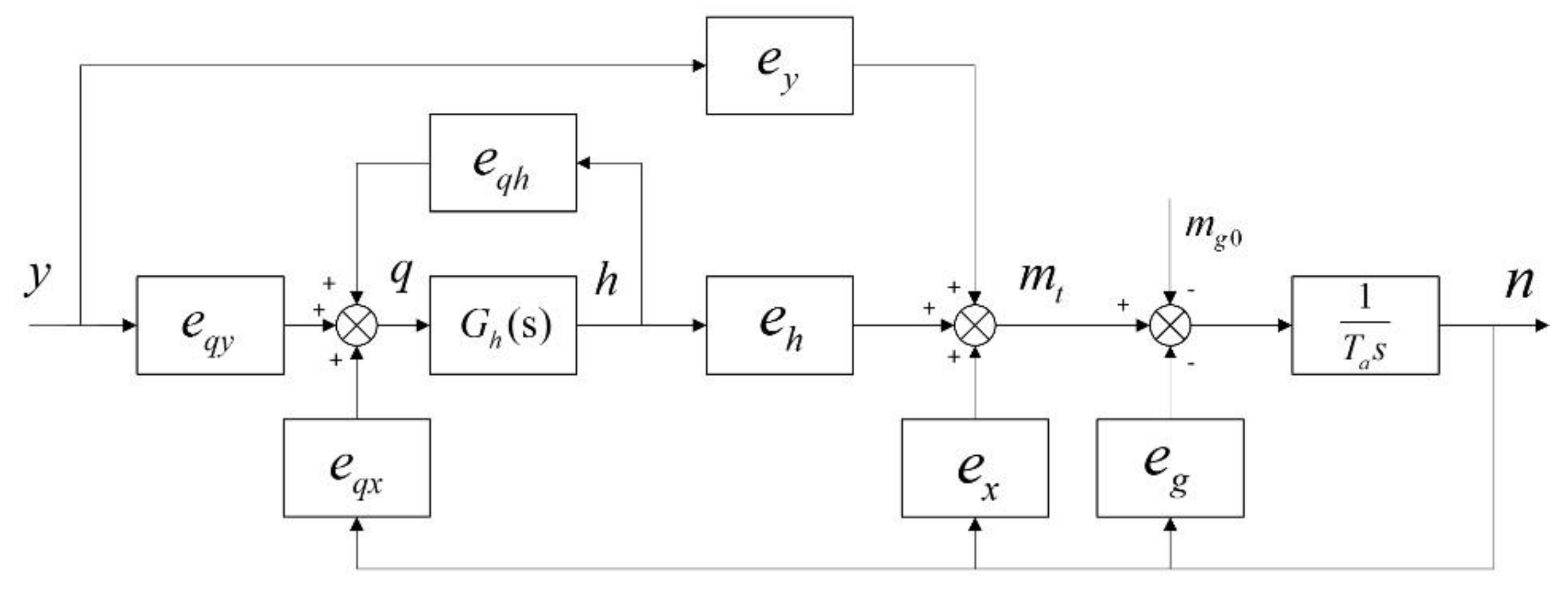
4. CAR Model of PSGM based on Precise Modeling of Water Diversion System

4.1. The Preliminary Transfer Function Based Order Determination of CAR Model

The structural schematic of the PSPP is illustrated in Figure 6. The overall generating/pumping system consists of the upper reservoir, long diversion pipeline, upstream surge tank, penstock, PSGM, draft tube, tailrace surge tank, tailrace tunnel and lower reservoir.

As the core installation for energy conversion in PSPP, PSGM can be viewed as a hydraulic-mechanical-electrical coupling system composed of the pump turbine and the synchronous generator-motor. Because the relationship between water head and flow rate in the pump turbine is directly affected by the water hammer effect in elastic water pipelines, the sophisticated dynamic characteristics of the components in the water diversion system must be considered in precise modeling of PSGM.

In order to express the precise analytical relation between water head and flow rate, the rigid water-hammer theory [9,40] is applied to generate differential equations that describe head-flow relations of the elements in the water diversion system. On the basis of accurate dynamic modeling of the elements in PSPP, six differential equations of the long diversion pipeline, upstream surge tank, pressure diversion pipe, draft tube, tailrace surge tank and tailrace tunnel are given in Equation (19):

$$\{\begin{array}{l}{\dot{q}}_2=(h_u^{\prime }-h_{s1}^{\prime })/T_{w2}\\ {\dot{h}}_{s1}=(q_2^{\prime }-q_t^{\prime })/T_{j1}\\ {\dot{q}}_t=(h_{s1}^{\prime }-h_{t1}^{\prime })/T_{w1}\\ {\dot{q}}_t=(h_{t2}^{\prime }-h_{s2}^{\prime })/T_{w4}\\ {\dot{h}}_{s2}=(q_t^{\prime }-q_3^{\prime })/T_{j2}\\ {\dot{q}}_3=(h_{s2}^{\prime }-h_d^{\prime })/T_{w3}\end{array}$$

(19)

where, $q_t$, $q_2$, $q_3$ denote the relative flow rate deviations of pump turbine, diversion tunnel and tailrace tunnel, respectively; $h_u^{\prime }=1+h_u$, $h_{s1}^{\prime }=1+h_{s1}$, $h_{s2}^{\prime }=1+h_{s2}$, $h_d^{\prime }=1+h_d$, $h_{t1}^{\prime }=1+h_{t1}$, $h_{t2}^{\prime }=1+h_{t2}$ represent the relative water heads of upper reservoir, upstream surge tank, tailrace surge tank, tailrace tunnel, lower reservoir, volute water inlet and volute water outlet, respectively; $T_{w1}$, $T_{w2}$, $T_{w3}$, $T_{w4}$ are the water inertia time constants of pressure diversion pipe, diversion tunnel, tailrace tunnel and draft tube, respectively.

The relative working head of the pump turbine $h_t=h_{t1}-h_{t2}$, thus the transfer function of the relative water head and flow rate of the pump turbine can be deduced from Equation (20):

$$G_h(\mathrm{s})=\frac{h_t(\mathrm{s})}{q_t(\mathrm{s})}=-\frac{a_5{\mathrm{s}}^5+a_3{\mathrm{s}}^3+a_1\mathrm{s}}{a_4{\mathrm{s}}^4+a_2{\mathrm{s}}^2+1}$$

(20)

where $a_1=T_{w1}+T_{w2}+T_{w3}+T_{w4}$, $a_2=T_{j1}{T}_{w2}+T_{j2}{T}_{w3}$, $a_3=T_{j1}{T}_{w2}(T_{w1}+T_{w3}+T_{w4})+T_{j2}{T}_{w3}(T_{w1}+T_{w2}+T_{w4})$, $a_4=T_{j1}{T}_{j2}{T}_{w2}{T}_{w3}$, $a_5=a_4(T_{w1}+T_{w4})$.

The block diagram of the PSGM is illustrated in Figure 7. It is seen that the torque $m_t$ and flow rate $q_t$ of the pump turbine could be expressed with six parameters closely related to the operating condition, as given in Equation (21):

$$\{\begin{array}{l}{m}_t(\mathrm{s})=e_y\cdot y(\mathrm{s})+e_x\cdot n(\mathrm{s})+e_h\cdot h_t(\mathrm{s})\\ q_t(\mathrm{s})=e_{qy}\cdot y(\mathrm{s})+e_{qx}\cdot n(\mathrm{s})+e_{qh}\cdot h_t(\mathrm{s})\end{array}$$

(21)

where y and n denote the relative guide vane opening and rotation speed of the pump turbine, respectively. $e_y$, $e_x$, $e_h$ are the first-order partial derivative of torque with respect to guide vane, rotor speed and water head, respectively; and $e_{qy}$, $e_{qx}$, $e_{qh}$ are the first-order partial derivative of flux with respect to guide vane, rotor speed and water head, respectively.

The transfer function of the synchronous generator-motor is simplified as a first-order inertia equation:

$$\frac{n(\mathrm{s})}{mt(\mathrm{s})-m_{g0}(\mathrm{s})}=\frac{1}{T_a\mathrm{s}+e_n}$$

(22)

From Equation (20) to Equation (22), the transfer function of the relative guide vane opening y and relative rotation speed n can be obtained as Equation (23):

$$\frac{n(\mathrm{s})}{y(\mathrm{s})}=e_y\frac{1+e{G}_h(\mathrm{s})}{\left(1-e_{qh}{G}_h(\mathrm{s})\right)\left(T_{a}s+e_n\right)}=\frac{b_5{\mathrm{s}}^5+b_4{\mathrm{s}}^4+b_3{\mathrm{s}}^3+b_2{\mathrm{s}}^2+b_1\mathrm{s}+e_y}{c_6{\mathrm{s}}^6+c_5{\mathrm{s}}^5+c_4{\mathrm{s}}^4+c_3{\mathrm{s}}^3+c_2{\mathrm{s}}^2+c_1\mathrm{s}+e_n}$$

(23)

where, $e_n=e_g-e_x$, $e=\frac{e_{qy}}{e_y}{e}_h-e_{qh}$, $b_1=-e_{y}e{a}_1$, $b_2=e_y{a}_2$, $b_3=-e_{y}e{a}_3$, $b_4=e_y{a}_4$, $b_5=-e_{y}e{a}_5$, $c_1=T_a+e_n{e}_{qh}{a}_1$, $c_2=T_a{e}_{qh}{a}_1+e_n{a}_2$, $c_3=T_a{a}_2+e_n{e}_{qh}{a}_3$, $c_4=T_a{e}_{qh}{a}_3+e_n{a}_4$, $c_5=T_a{a}_4+e_n{e}_{qh}{a}_5$, $c_6=T_a{e}_{qh}{a}_5$.

System models are usually discretized in engineering practice according to sampling intervals of computer system. A discrete-time CAR model [41] in which the input vector is made up of a certain combination of the historical system inputs and outputs at past few sampling instants, is naturally obtained by applying z-transform to the continuous transfer function Equation (23). Here, the CAR model of PSGM is given in Equation (24):

$$n(k)={\displaystyle \sum _{i=1}^{n_a}{\xi }_n(i)n(k-i)}+{\displaystyle \sum _{j=0}^{n_b}{\xi }_y(j)y(k-j)}$$

(24)

where, the first term on the right side of Equation (24) is the autoregressive part and second term is the controlled part of CAR. n_a and n_b denote the order of numerator and denominator the z-transform of Equation (23), respectively; ${\xi }_n$, ${\xi }_y$ represent the corresponding coefficient of the rotation speed and guide vane opening in the sequence, respectively. Therefore, the vector $\left[n(k-1)n(k-2)\cdots n(k-n_a)y(k)y(k-1)\cdots y(k-n_b+1)\right]$ and n(k) are preliminarily selected as the input and output of the CAR model of PSGM, where $n_a=5$ and $n_b=6$ are naturally obtained according to Equations (23) and (24).

4.2. Parameter Reduction Using F-Test Strategy

The preliminary determination of system order in Section 4.1 has found out the upper boundaries of the length of autoregressive and controlled parts in CAR, but modeling details such as the time delay of the system and the redundant parameters in the two parts still need further analysis. According to the economical principle, fewer parameters are expected to be included in the system model under the premise of modeling accuracy for its structural simplicity. In order to precisely describe the system dynamics with fewer number of parameters, a detailed parameter reduction method based on the well-known F-test [42,43,44] is utilized after the preliminary system order determination. The parameter reduction process based on F-test strategy can be divided into three parts. At first, the time delay of the system input is determined. Then, the redundant parameters in the controlled term are discarded considering the system time delay. Finally, the redundant parameters in the auto-regressive term are also eliminated considering the reduction in controlled term. With these operations, the economical parameter model of PSGM is obtained.

Suppose there exists n sets of input-output data for the PSGM described by the CAR model deduced in Section 4.1, it’s apparent that the classic RLS method can be used to identify the model parameters, so the model outputs $\hat{y}(i)$ can be obtained and the residual sum of squares of the model can be expressed as Equation (25):

$$S={{\sum }_{i=1}^n\left(y(i)-\hat{y}(i)\right)}^2$$

(25)

The F-test judgment of redundant parameters of CAR model is given in the following:

Assume $S_1$ as the residual sum of squares of the complete model and $S_2$ the residual sum of squares of the model in which some parameters X (the vector $X=\left(x_1,x_2,\cdots ,x_m\right)$ denotes the parameters to be discarded in CAR model) are deleted compared with the complete model. The statistical variable F is defined as Equation (26) [42]:

$$F=\frac{S_2-S_1}{S_1}\cdot \frac{n-n_1}{n_1-n_2}$$

(26)

where, n denotes the number of sampling data, $n_1$ denotes the total number of parameters in the complete CAR model (i.e., $n_1=n_a+n_b+1$) and $n_2$ is the number of remaining parameters in the economical model.

F approachably subjects to $F(n_1-n_2,n-n_1)$ distribution. When the significance level is chosen to be 0.05, according to the F distribution table, we can obtain the corresponding critical value $F_{\alpha }$. If $F<F_{\alpha }$, then the economical parameter model is considered acceptable (which means the deleted parameters are statistically insignificantly different from zero); else, the economical parameters model is considered unacceptable (which means there exists at least one parameter that shouldn’t be deleted).

The detailed processes of parameter reduction are listed below:

Step 1:

Determine the time delay of the original CAR model $M_0$: delete the parameters in the controlled term one by one successively from $y(k)$ to $y(k-n_b)$ by iterations. In the i-th iteration, whether the parameter $y(k-i+1)$ should be deleted or not is judged by two F-tests. The economical parameter CAR model without $y(k-i)$ is used to make comparison with the economical parameter CAR model with $y(k-i)$ and original CAR model $M_0$ with no parameter discarded, respectively. Only if both of the two F-test results are acceptable, the parameter $y(k-i)$ can be deleted from the controlled parameter sequence. And then the time delay is updated as $\tau =i$. Once the $y(k-i)$ is considered to be preserved in the CAR model (namely anyone of the two F-tests is not passed), the iterations of time delay are ended and the time delay is set as $\tau =i-1$.

Step 2:

Record the economical parameter model as $M_1$ considering the time delay determined by Step 1.

Step 3:

Determine the redundant controlled parameters: delete the rest controlled parameters one by one in $M_1$ in the inverted order from $y(k-n_b)$ to $y(k-\tau -1)$ by iterations. In the j-th iteration, whether $y(k-n_b-j+1)$ should be deleted from $M_1$ is judged by the F-test between the economical parameter model with the parameter $y(k-n_b-j+1)$ and the economical parameter model without it. If $F<F_{\alpha }$, $y(k-n_b-j+1)$ can be deleted from $M_1$ due to the parameter-saving principle, then replace $M_1$ with the economical model without the parameter $y(k-n_b-j+1)$ and go to the next iteration. Else, the parameter $y(k-n_b-j+1)$ should be preserved in $M_1$ and step to the next iteration.

Step 4:

Record the economical parameter model as $M_2$ considering both the time delay determined by Step 1 and the redundant controlled parameters reduction by Step 3.

Step 5:

Determine the redundant autoregressive parameters: delete the autoregressive parameters one by one in $M_2$ in the inverted order from $n(k-n_a)$ to $n(k-1)$ by iterations. In the p-th iteration, whether $n(k-n_a-p+1)$ should be deleted from $M_2$ is judged by the F-test between the economical model with the parameter $n(k-n_a-p+1)$ and the economical model without it. If $F<F_{\alpha }$, $n(k-n_a-p+1)$ can be deleted from $M_2$, then replace $M_2$ with the economical model without the parameter $n(k-n_a-p+1)$ and go to the next iteration. Else, the parameter $n(k-n_a-p+1)$ should be preserved in $M_2$ and step to the next iteration.

Step 6:

Record the economical parameter model as $M_3$ considering the time delay, the redundant parameters of both autoregressive and controlled parameters. $M_3$ is therefore considered as the final economical parameter CAR model of PSGM system.

4.3. The Issues for Model Application in PSGM

In the T-S fuzzy model of PSGM system, the input vector $\left[n(k-1)n(k-2)\cdots n(k-n_a)y(k)y(k-1)\cdots y(k-n_b+1)\right]$ consists of a certain combination of rotation speeds and guide vane openings at the last few time samples and the output is the rotor speed at the current sampling time. The dimensional coefficients $n_a$ and $n_b$ are chosen as $n_a=5$, $n_b=6$ from the discrete-time precise CAR model of PSGM discussed in Section 4.1, which means the model input is $\left[n(k-1)n(k-2)\cdots n(k-5)y(k)y(k-1)\cdots y(k-5)\right]$. However, the preliminarily suggested values of $n_a$ and $n_b$ in Section 4.1 make it a relatively higher dimensional (11-dimensional) time-series model and can be viewed as their upper bounds, so more model training work should be done to simplify the CAR model and determine the most appropriate parameters in it with F-test based parameter reduction strategy in Section 4.2.

In this paper, the training samples of PSGM are chosen from the condition experimental data of a PSPP in Central China which comprise 900 sets of practical data containing the guide vane openings and the rotor speeds under different working conditions. The detailed composing form of the training samples is listed in

Table 2. Detailed composition of the training samples for T-S modeling.

Condition Name	Number of Samples
Start-up to no-load operating process	150
Synchronizing process to rated load operation	200
Shut down process in generation direction	50
Load rejection from rated load state	250
Pump start to rated power in pumping direction	20
Shut down process in pumping direction	30
Pumping convert to generation transients	200

.

With the application of the presented parameter reduction method, the parameters $n(k-4)$, $n(k-5)$, $y(k)$, $y(k-3)$, $y(k-4)$, $y(k-5)$ in the previous input vector are considered redundant and determined to be discarded. Thus, the ultimate input of the CAR model is chosen as a 5-dimensional vector, i.e., $\left[n(k-1)n(k-2)n(k-3)y(k-1)y(k-2)\right]$ with acceptable training errors. The training errors are shown in Figure 8.

5. Model Validation and Result Analysis

In order to validate the accuracy and adaptation of the proposed T-S fuzzy model for PSGM, comparative studies have been conducted under three typical operating conditions in PSPP using the proposed T-S fuzzy model and the traditional mechanistic model, respectively. The mechanistic model for comparative study adopts the well-known method of characteristics to tackle the sophisticated dynamics in the water diversion system of PSPP and the interpolation in complete characteristic curves to obtain the rotation speed and the flow rate under different operating conditions, where the detailed modeling description can be found in [45]. The detailed parameter information of the PSGM and its water diversion system for mechanistic modeling is given in Appendix. In this section, simulation results of the two modeling approaches are compared with the practical rotation speed curves obtained from the signal recording system in the PSPP under the corresponding conditions. All the units of input and output variables are converted to per unit (pu).

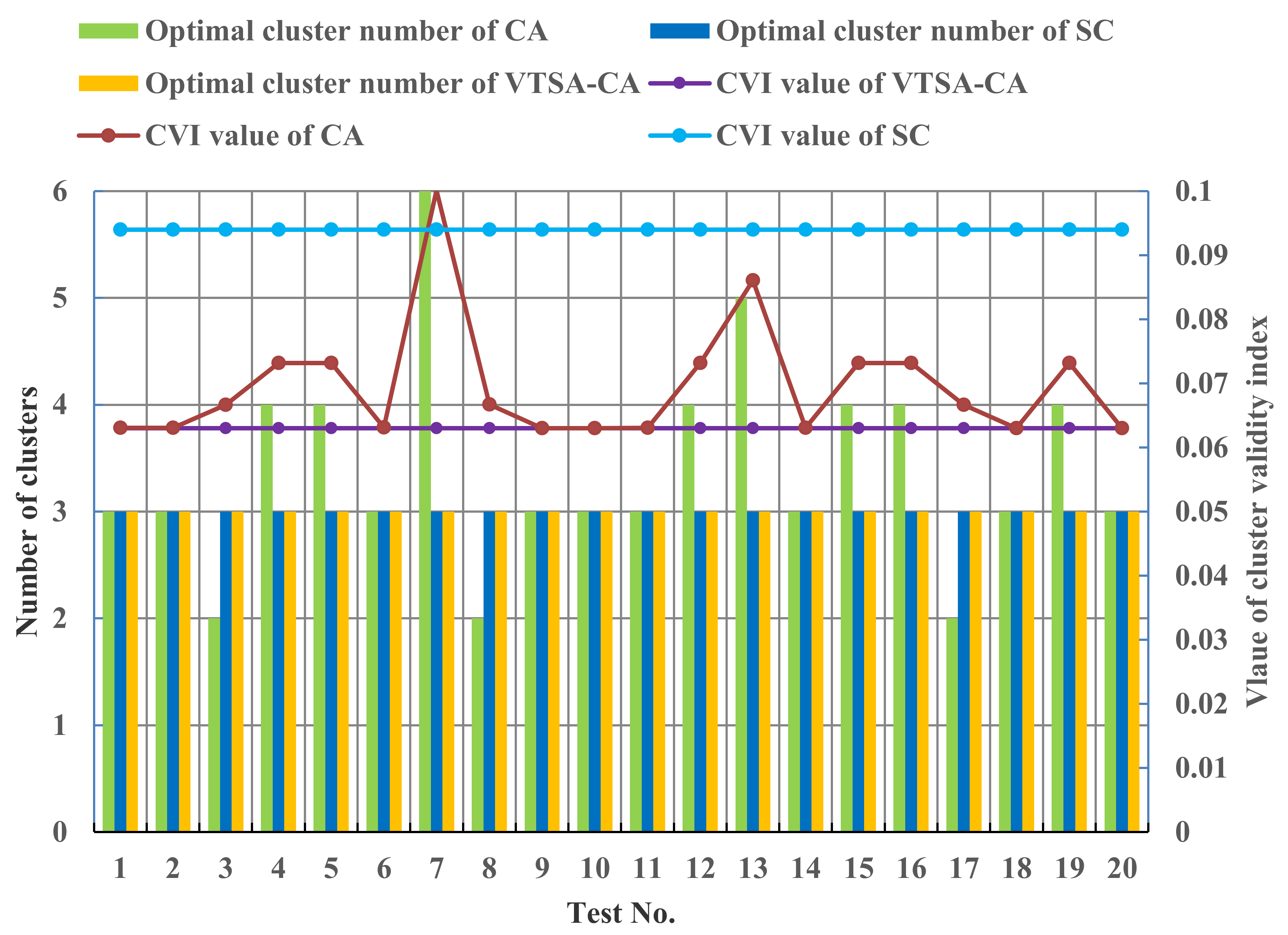
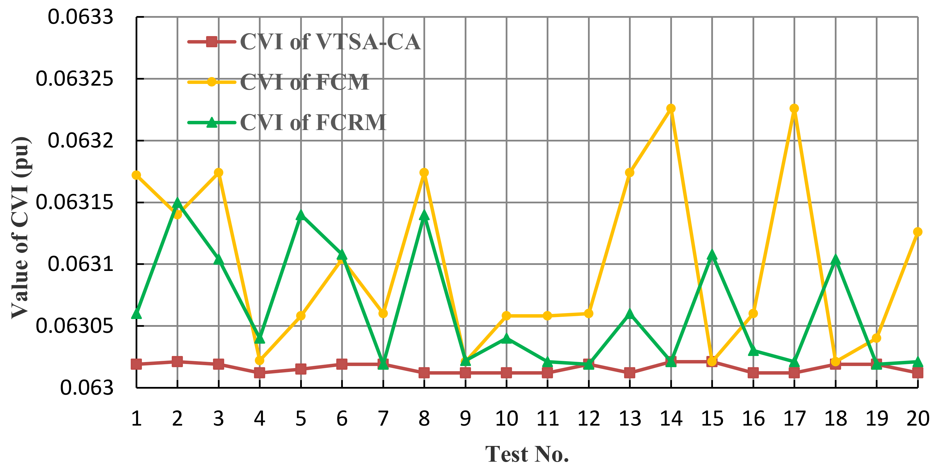
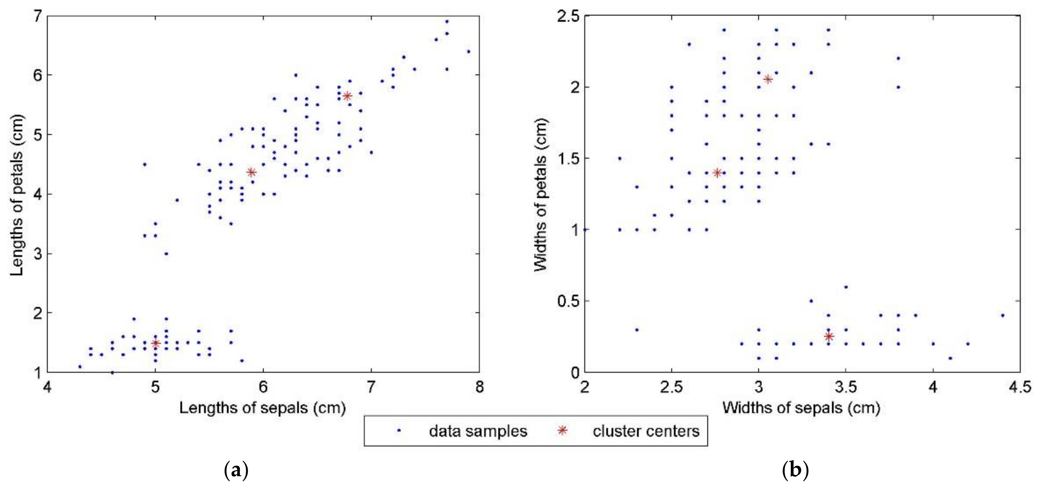
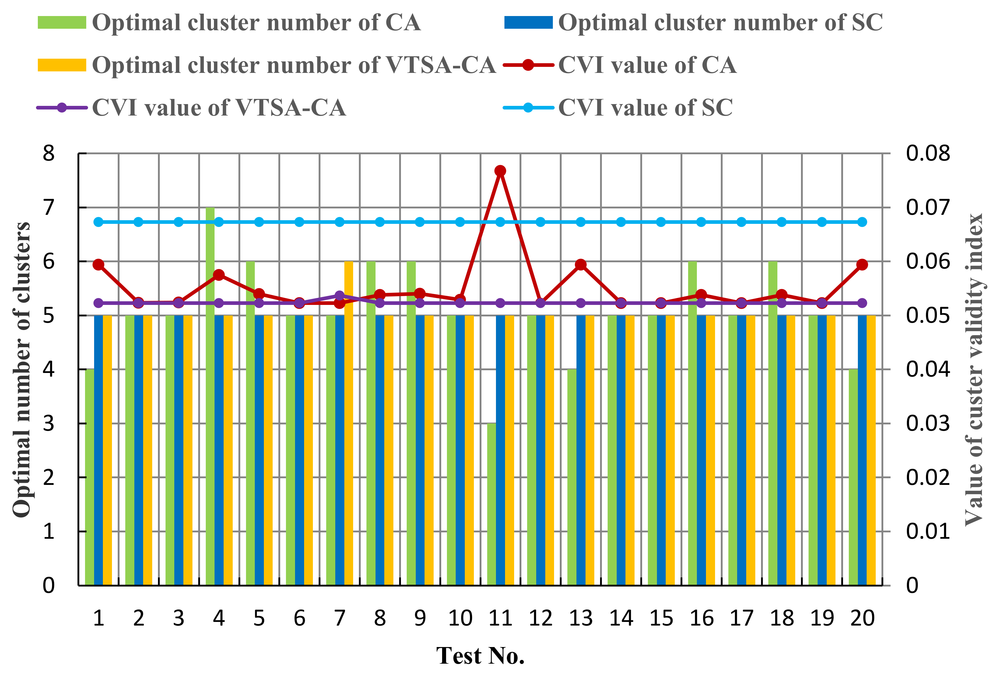
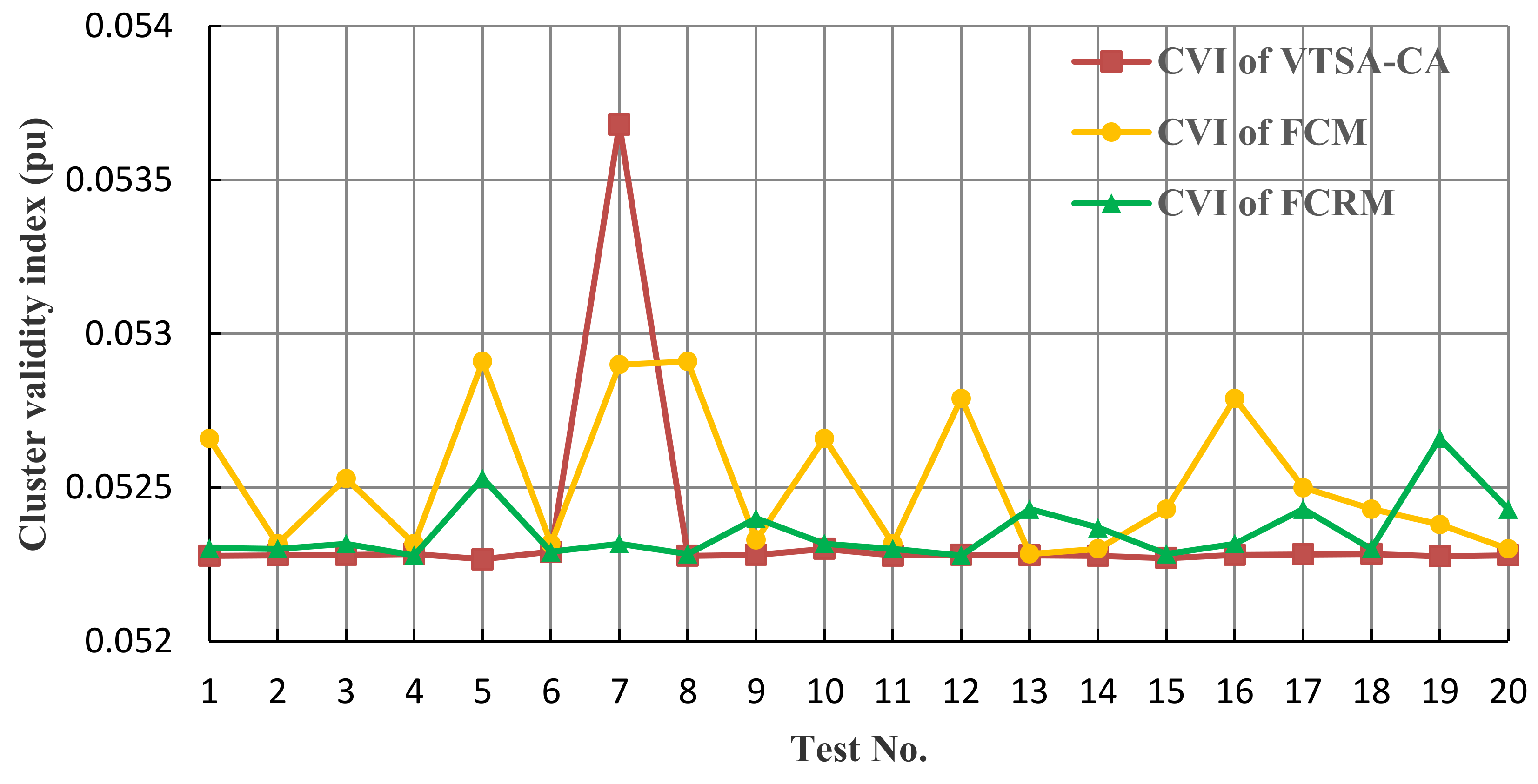
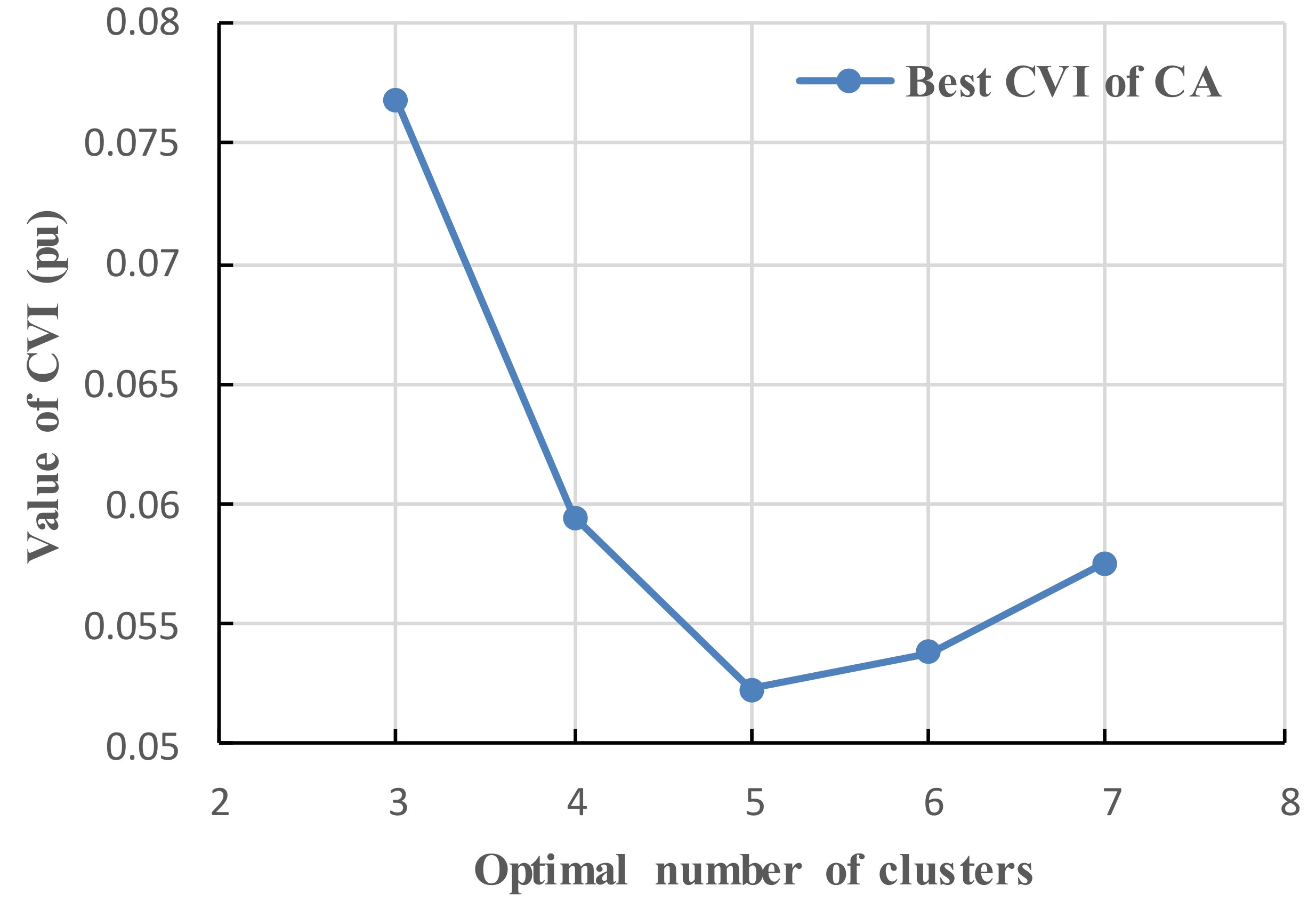
5.1. Results of the Premise Identification of T-S Fuzzy Model

Considering the value ranges of the rotation speed and guide vane opening in all aforementioned working conditions, the parameters setting of the proposed TSA-CA based T-S fuzzy model is given below:

The search space for clustering centers $v_{ik}$ is set as $v_{ik}\in [-1,1]$, for $k=1,2,\cdots ,n_a$ and $v_{ik}\in [0,1]$ for $k=n_a+1,n_a+2,\cdots ,n_a+n_b$ according to the value ranges of rotor speed and guide vane opening, respectively. The search tendency $ST=0.3$, the tree population size $popSize=40$, the maximum generation $maxGen=50$, and the seed generation rate ranges from 10% to 20% of the tree population size. In addition, as a rule of thumb, the cluster number ranges within $c\in [2,\sqrt{n}]$, where n denotes the total number of training samples.

(1) The optimization stability of VTSA-CA

As the determination of the optimal cluster number c which determines the number of fuzzy rules is one of the difficulty in T-S fuzzy modeling, the VTSA-CA algorithm is introduced to specify the optimal number of clusters and the best fuzzy partition of the system. The cluster number c with the smallest value of CVI tends to have the clearest clustering distribution and should be adopted as the number of fuzzy rules in the proposed T-S fuzzy model. In this paper, the premise parameter identification experiments for different values of c have been repeated for twenty times with SC, FCM, FCRM, CA and VTSA-CA to attenuate the contingency and stochastic influences of the results, respectively. The optimization results of CVI and the optimal cluster numbers determined by SC, CA and VTSA-CA are presented in Figure 9.

It can be seen from Figure 9 that the optimal c obtained by basic CA ranges from [3,7], which indicates that uncertainty exists in searching for the most appropriate fuzzy partition. Although SC could obtain the optimal number of clusters, its CVI values are much greater than those of other methods, indicating its incapability in finding optimal fuzzy distribution. However, the optimization results of VTSA-CA appears much more stable and the optimal number of clusters is obtained in 19 of 20 experiments.

By defining the number of clusters $c=5$, FCM and FCRM are utilized as comparative methods to testify the fuzzy partition performance of VTSA-CA. The CVI values in 20 experiments are illustrated in Figure 10. Apart from Test No.7 where the $c=5$ failed to be searched, the CVIs of VTSA-CA outperform those of comparative methods in all other tests. It shows the superiority of VTSA-CA in global exploration aspects.

(2) The optimal number of clusters determination

The optimization stability increases in VTSA-CA by introducing a CVI (given in Equation (10A)) into the global optimization to judge the performance of the fuzzy clustering and thus determine the optimal choice of c. In Figure 9, it can be clearly seen that $c=5$ is chosen as the optimal number of clusters by VTSA-CA. The best CVI values for different choice of c by CA are illustrated in Figure 11 and the CVI in the case of $c=5$ has the minimal value, which means that VTSA-CA is able to make an accurate judgment in optimal cluster number determination.

The variations of the number of clusters in different optimization processes are depicted in Figure 12. We select 5 experiments by CA where the results of the optimal number of clusters range from [3,7] and an experiments by VTSA-CA where the optimal c is correctly obtained as c = 5. Note that only the results of the first 20 iterations in the experiments are displayed because the optimal number of clusters is convergent and no longer changes thereafter. It can be found that the convergence rate of VTSA-CA is faster than that of CA. Furthermore, it should be emphasized that the optimal c is 5 in the 10th iteration and increases back to c = 6 in the 11th iteration because of the variable string length property in VTSA-CA, which obviously strengthen the global exploration capability and solve the intrinsic defect of monotonically decrease in cluster number in the searching process of CA.

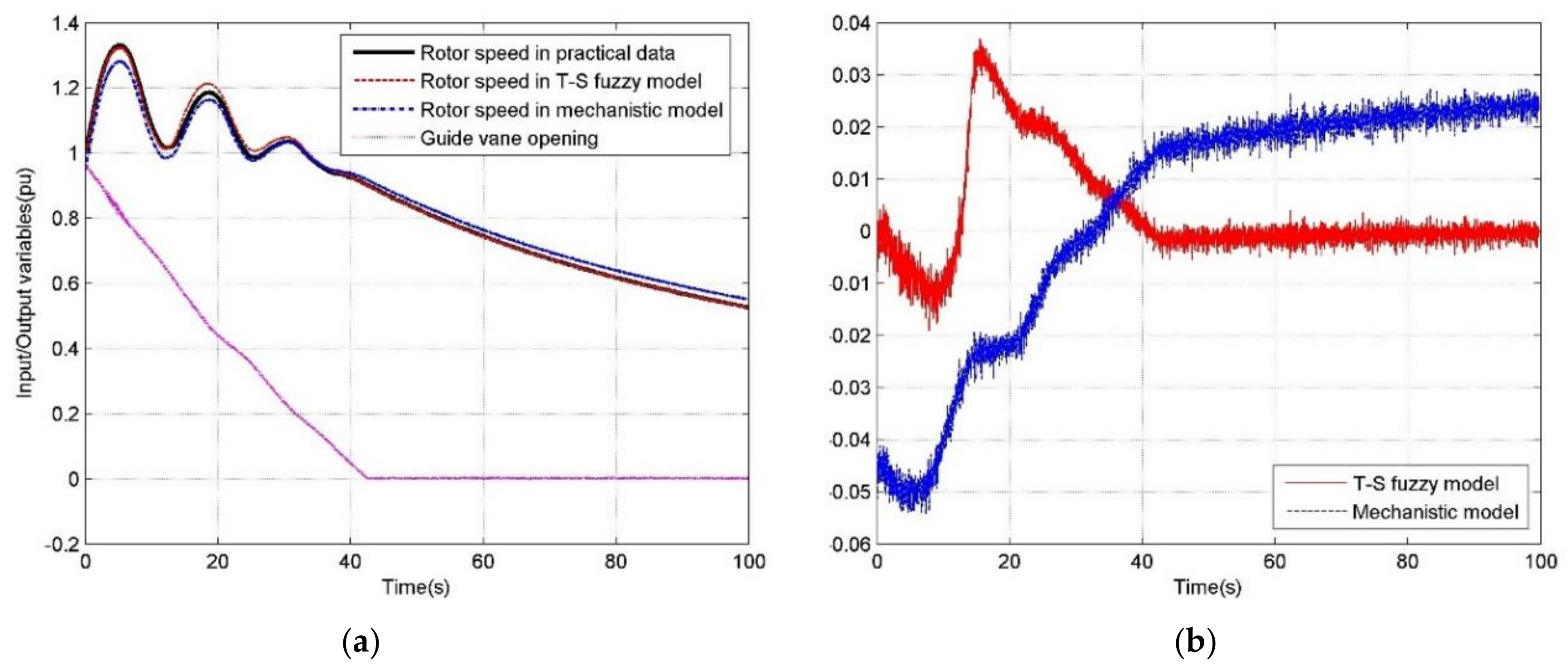
5.2. Simulations under Different Operating Conditions

For the sake of validating the accuracy of the T-S fuzzy model for PSGM and its superiority in comparison with the traditional mechanistic model, three typical operating transients, i.e., the normal start and connection to power grid process in generation direction, the load rejection process at the rated condition and the transients of rated pumping condition convert to generation direction, have been simulated with the proposed T-S fuzzy model and the traditional mechanistic model, respectively. By comparing the simulation results of the two models with the corresponding practical data, the models precision can be specified.

(1) Case A: dynamic process in power generation direction.

The dynamic process in power generation direction of PSGM consists of the start-up of hydraulic turbine, the synchronization and the steady operation with rated load. In this simulation, dynamic input data of guide vane opening at every sample and the initial input data of rotation speed at the first sample are obtained from practical machine experiments. Rotation speed of the proposed T-S fuzzy model, the traditional mechanistic model and the practical data as well as speed errors compared with the practical data in power generation direction are shown in Figure 13a,b, respectively.

From Figure 13a, we can clearly find that the T-S fuzzy model performs much better in simulation accuracy. Obvious simulated rotation speed errors appears when the PID controller cut in under the no-load condition for the mechanistic model while T-S model possesses stronger tracking capability. The error in Figure 13b is mainly caused by simplification of the nonlinear factors in servo actuator model such as backlash and dead-zone nonlinearity in the traditional mechanistic model. The data-based T-S fuzzy model could overcome the hardship in precisely describing the nonlinearities in PSGM. The performance indexes of the two models under normal power generation condition, including maximal error (Max Error), minimal error (Min Error), sum of square error (SSE), mean square error (MSE), root mean square error (RMSE) and mean absolute percentage error (MAPE), are given in

Table 3. Performance indexes of the two models under normal power generation condition.

Model	Max Error	Min Error	SSE	MSE	RMSE	MAPE (%)
Mechanistic	0.0277	0	0.5661	9.450 × 10−5	0.0097	2.2879
T-S fuzzy	0.0081	1.021 × 10−6	0.0267	4.457 × 10−6	0.0021	0.5517

. We can clearly find that T-S fuzzy model outperforms the mechanistic model in modeling precision.

(2) Case B: load rejection condition

Load rejection condition consists of the quick close-down of the wicket gate and the oscillatory decrease of the rotor speed after cutout of the generator circuit breaker (GCB). The practical and simulation results of rotation speed of PSGM in this condition are illustrated in Figure 14a. It is difficult for the traditional mechanistic model to precisely simulate the overall dynamic behaviors in this condition because the drastic flow rate and water-head fluctuations in the water diversion system may amplify the modelling error of PSGM.

As shown in Figure 12b, absolute output error lasts for the whole process using traditional mechanistic model while the error attenuates to zero after the rotation speed oscillations at the beginning of the load rejection transients simulated by the proposed T-S fuzzy model. The performance indexes of the two models under load rejection condition are given in

Table 4. Performance indexes of the two models under load rejection condition.

Model	Max Error	Min Error	SSE	MSE	RMSE	MAPE (%)
Mechanistic	0.0542	1.425 × 10−5	2.893	5.797 × 10−4	0.0241	2.6416
T-S fuzzy	0.0370	1.096 × 10−6	0.552	1.106 × 10−4	0.0105	0.6149

, which quantitatively indicate the superiority of the T-S fuzzy model.

(3) Case C: conversion process from pumping to power generation

The conversion process from pumping to power generation is a unique operating condition for PSGM. The guide vane opening firstly decreases linearly to a certain transfer opening about 0.08 pu before the rotation speed start to decrease in pumping direction from the rated speed gradually to zero and then reverse to increase in power generation direction (Note that the rotational direction of the rotor in power generation condition is stipulated as the positive direction in this paper). The guide vane opening starts increasing from the transfer opening to start opening limitation when the positive speed reaches 0.65 and the PID controller cut in when rotation speed reaches 0.85. The practical and simulation results and model errors compared with practical data are given in Figure 15a,b, respectively. The T-S fuzzy model also performs better than the traditional mechanistic model in this transient process, which indicates the superiority and adaptation of the proposed T-S model for PSGM again. From the performance indexes of the two models given in

Table 5. Performance indexes under pumping convert to power generation condition.

Model	Max Error	Min Error	SSE	MSE	RMSE	MAPE (%)
Mechanistic	0.0376	0	1.1276	1.599 × 10−4	0.0126	6.1434
T-S fuzzy	0.0234	3.14 × 10−6	0.2243	3.182 × 10−5	0.0056	1.2219

, the T-S fuzzy model is also proved to achieve better modeling precision than the mechanistic one under pumping convert to power generation condition.

6. Conclusions

In traditional fuzzy cluster methods such as FCM and FCRM, the number of clusters needs to be defined a priori and the locations of cluster centers are easily trapped in local optima due to their gradient-based solution searching property. In view of the two main deficiencies that exist, a novel swarm intelligence fuzzy clustering algorithm called VTSA-CA is proposed in this paper. VTSA-CA is capable of determining an appropriate number of clusters automatically during the optimization process. And it possesses a comprehensive optimization mechanism in which the global exploration ability of TSA and the local exploitation property of CA interact with each other to obtain the global best fuzzy cluster distribution. The novel clustering algorithm is naturally incorporated in the premise identification of T-S model for its excellent nonlinear behavior fitting capability. For the sake of utilizing the proposed T-S fuzzy model to precisely reflect the input-output relation of PSGM, an economical parameter CAR model is deduced. The input and output boundaries of the CAR model are preliminarily determined by a high-order transfer function of PSGM considering the distributed components in the water diversion system. Then an F-test based redundant parameter reduction strategy is utilized to determine the time delay and discard the redundant parameters in the CAR model. The input and output formats of the CAR model are set as the input and output of the T-S fuzzy model. Comparative studies have been conducted in diverse typical operating conditions in PSPP to validate the effectiveness of the proposed T-S fuzzy model as well as its superiority over the traditional mechanistic model. The output of the proposed T-S fuzzy model for PSGM is a linear combination of the system inputs, rather than complex nonlinear mathematical expressions in the traditional mechanistic model. Furthermore, the model training process is completed offline with practical data in a special CAR model formulation, which greatly attenuates the online computational burden while ensuring the model accuracy simultaneously.

References

1. Yang, W.; Yang, J.; Guo, W.; Zeng, W.; Wang, C.; Saarinen, L.; Norrlund, P. A Mathematical Model and Its Application for Hydro Power Units under Different Operating Conditions. Energies 2015, 8, 10260–10275. [Google Scholar] [CrossRef]
2. Chaudhry, M. Applied Hydraulic Transients; Van Nostrand Reinhold Co.: New York, NY, USA, 1979. [Google Scholar]
3. Derakhshan, S.; Nourbakhsh, A. Experimental study of characteristic curves of centrifugal pumps working as turbines in different specific speeds. Exp. Therm. Fluid Sci. 2008, 32, 800–807. [Google Scholar] [CrossRef]
4. Yoo, I.; Park, M.; Hwang, S.; Yoon, E. Complete Characteristic Curve for a Reactor Coolant Pump. J. Fluid Mach. 2012, 15, 5–10. [Google Scholar] [CrossRef]
5. Zheng, X.; Guo, P.; Tong, H.; Luo, X. Improved Suter-transformation for complete characteristic curves of pump-turbine. In Proceedings of the 26th Iahr Symposium On Hydraulic Machinery And Systems, Beijing, China, 19–23 August 2012; Volume 15, p. 062015. [Google Scholar]
6. Izquierdo, J.; Iglesias, P. Mathematical modelling of hydraulic transients in simple systems. Math. Comput. Model. 2002, 35, 801–812. [Google Scholar] [CrossRef]
7. Nicolet, C.; Greiveldinger, B.; Herou, J.; Kawkabani, B.; Allenbach, P.; Simond, J.; Avellan, F. High-Order Modeling of Hydraulic Power Plant in Islanded Power Network. IEEE Trans. Power Syst. 2007, 22, 1870–1880. [Google Scholar] [CrossRef]
8. Sim, W.G.; Park, J. Transient analysis for compressible fluid flow in transmission line by the method of characteristics. J. Mech. Sci. Technol. 1997, 11, 173–185. [Google Scholar] [CrossRef]
9. Souza, O.H.; Barbieri, N.; Santos, A. Study of hydraulic transients in hydropower plants through simulation of nonlinear model of penstock and hydraulic turbine model. IEEE Trans. Power. Syst. 1999, 14, 1269–1272. [Google Scholar] [CrossRef]
10. Fang, H.; Chen, L.; Dlakavu, N.; Shen, Z. Basic Modeling and Simulation Tool for Analysis of Hydraulic Transients in Hydroelectric Power Plants. IEEE Trans. Energy Convers. 2008, 23, 834–841. [Google Scholar] [CrossRef]
11. Guo, W.; Yang, J.; Chen, J.; Wang, M. Nonlinear modeling and dynamic control of hydro-turbine governing system with upstream surge tank and sloping ceiling tailrace tunnel. Nonlinear Dyn. 2016, 84, 1383–1397. [Google Scholar] [CrossRef]
12. Li, C.; Zhou, J. Parameters identification of hydraulic turbine governing system using improved gravitational search algorithm. Energy Convers. Manag. 2011, 52, 374–381. [Google Scholar] [CrossRef]
13. Strah, B.; Kuljaca, O.; Vukic, Z. Speed and active power control of hydro turbine unit. IEEE Trans. Energy Convers. 2005, 20, 424–434. [Google Scholar] [CrossRef]
14. Zeng, W.; Yang, J.; Yang, W. Instability analysis of pumped-storage stations under no-load conditions using a parameter-varying model. Renew. Energy 2016, 90, 420–429. [Google Scholar] [CrossRef]
15. Liu, Y.; Fang, Y. BGNN Neural Network Based on Improved E.Coli Foraging Optimization Algorithm Used in the Nonlinear Modeling of Hydraulic Turbine. Int. Symp. Neural Netw. Adv. Neural Netw. 2009, 5551, 624–634. [Google Scholar]
16. Yi, J.; Yan, J.; Fang, X. Modeling of hydraulic turbine systems based on a Bayesian-Gaussian neural network driven by sliding window data. Front. Inf. Technol. Electron. Eng. 2010, 11, 56–62. [Google Scholar]
17. Chen, R.; Zhen, J.; Liu, Y. Inverse Model Design of Hydraulic Turbine System Using Bayesian Inferring Method. Intell. Syst. 2011, 2, 87–91. [Google Scholar]
18. Lin, L.; Zhong, S.; Xie, X. A Type Design Method of Large Hydraulic Turbine Based on the Gaussian Mixture Model. Prz. Elektrotechniczn. 2012, 88, 153–156. [Google Scholar]
19. Zhong, S.; Wang, T.; Ding, G.; Bu, L. Multi-attribute grey fuzzy optimized decision-making model of large-scale hydraulic turbine design scheme. Comput. Integr. Manuf. Syst. 2008, 14, 1905–1912. [Google Scholar]
20. Li, C.; Zhou, J.; Xiang, X.; Li, Q.; An, X. T–S fuzzy model identification based on a novel fuzzy c-regression model clustering algorithm. Eng. Appl. Artif. Intell. 2009, 22, 646–653. [Google Scholar] [CrossRef]
21. Li, C.; Zhou, J.; Xiao, J.; Xiao, H. Hydraulic turbine governing system identification using T–S fuzzy model optimized by chaotic gravitational search algorithm. Eng. Appl. Artif. Intell. 2013, 26, 2073–2082. [Google Scholar] [CrossRef]
22. Sugeno, M.; Yasukawa, T. A fuzzy-logic-based approach to qualitative modeling. IEEE Trans. Fuzzy Syst. 1993, 1, 7. [Google Scholar] [CrossRef]
23. Kim, E.; Park, M.; Ji, S.; Park, M. A new approach to fuzzy modeling. IEEE Trans. Fuzzy Syst. 1997, 5, 328–337. [Google Scholar]
24. Kim, E.; Park, M.; Kim, S.; Park, M. A transformed input-domain approach to fuzzy modeling. IEEE Trans. Fuzzy Syst. 1998, 6, 596–604. [Google Scholar]
25. Du, H.; Zhang, N. Application of evolving Takagi-Sugeno fuzzy model to nonlinear system identification. Appl. Soft Comput. 2008, 8, 676–686. [Google Scholar] [CrossRef]
26. Du, Y.; Lu, X.; Chen, L.; Zeng, W. An interval type-2 T-S fuzzy classification system based on PSO and SVM for gender recognition. Multimedia Tools Appl. 2016, 75, 987–1007. [Google Scholar] [CrossRef]
27. Su, Z.; Wang, P.; Shen, J.; Zhang, Y.; Chen, L. Convenient T–S fuzzy model with enhanced performance using a novel swarm intelligent fuzzy clustering technique. J. Process Control 2012, 22, 108–124. [Google Scholar] [CrossRef]
28. Niu, B.; Li, L. Design of T-S Fuzzy Model Based on PSODE Algorithm. Int. Conf. Intell. Comput. 2008, 5227, 384–390. [Google Scholar]
29. Su, H.; Yang, Y. Differential evolution and quantum-inquired differential evolution for evolving Takagi–Sugeno fuzzy models. Expert Syst. Appl. 2011, 38, 6447–6451. [Google Scholar] [CrossRef]
30. Frigui, H.; Krishnapuram, R. Clustering by competitive agglomeration. Pattern Recogn. 1997, 30, 1109–1119. [Google Scholar] [CrossRef]
31. Gandy, L.; Rahimi, S.; Gupta, B. A modified competitive agglomeration for relational data algorithm. In Proceedings of the Annual Meeting of the North-American-Fuzzy-Information-Processing-Society, Detroit, MI, USA, 26–28 June 2005; pp. 210–215. [Google Scholar]
32. Jeng, J.; Chuang, C.; Tao, C. Interval competitive agglomeration clustering algorithm. Int. J. Fuzzy Syst. 2010, 37, 6567–6578. [Google Scholar] [CrossRef]
33. Zhao, L.; Qian, F.; Yang, Y.; Zeng, Y.; Su, H. Automatically extracting T–S fuzzy models using cooperative random learning particle swarm optimization. Appl. Soft Comput. 2010, 10, 938–944. [Google Scholar] [CrossRef]
34. Srikanth, R.; George, R.; Warsi, N.; Prabhu, D.; Petry, F.; Buckles, B. A variable-length genetic algorithm for clustering and classification. Pattern Recogn. Lett. 1995, 16, 789–800. [Google Scholar] [CrossRef]
35. Sjahputera, O.; Scott, G.; Claywell, B.; Klaric, M.N.; Hudson, N.J.; Keller, J.M.; Davis, C.H. Clustering of Detected Changes in High-Resolution Satellite Imagery Using a Stabilized Competitive Agglomeration Algorithm. IEEE Trans. Geosci. Remote Sens. 2011, 49, 4687–4703. [Google Scholar] [CrossRef]
36. Kiran, M.S. TSA: Tree-seed algorithm for continuous optimization. Expert Syst. Appl. 2015, 42, 6686–6698. [Google Scholar] [CrossRef]
37. Kiran, M.S. An Implementation of Tree-Seed Algorithm (TSA) for Constrained Optimization. In Proceedings of the 19th Asia Pacific Symposium on Intelligent and Evolutionary Systems, Bangkok, Thailand, 22–25 November 2016; Volume 5, pp. 189–197. [Google Scholar]
38. Takagi, T.; Sugeno, M. Fuzzy Identification of Systems and Its Applications to Modeling and Control. IEEE Trans. Syst. Cybern. 1985, 15, 387–403. [Google Scholar] [CrossRef]
39. Pang, Z.; Cui, H. System Identification and Adaptive Control: The MATLAB Simulation, 1st ed.; Beijing University of Aeronautics and Astronautics Press: Beijing, China, 2009. [Google Scholar]
40. Zeng, Y.; Guo, Y.; Zang, L.; Xu, T.; Dong, H. Nonlinear hydro turbine model having a surge tank. Math. Comput. Model. Dyn. Syst. 2012, 19, 1–17. [Google Scholar] [CrossRef]
41. Rawlings, J.; Mayne, D. Model Predictive Control: Theory and Design; Nob Hill Publishing LLC: Madison, WI, USA, 2000; pp. 3430–3433. [Google Scholar]
42. Deng, Z. Structure Identification Of Multivariable Carma Models. Acta Autom. Sin. 1986, 12, 18–24. [Google Scholar]
43. Wang, S.; Cui, H. Generalized F test for high dimensional linear regression coefficients. J. Multivar. Anal. 2013, 117, 134–149. [Google Scholar] [CrossRef]
44. Steinberger, L. The relative effects of dimensionality and multiplicity of hypotheses on the F-test in linear regression. Electron. J. Stat. 2016, 10, 2584–2640. [Google Scholar] [CrossRef]
45. Li, C.; Mao, Y.; Yang, J.; Wang, Z.; Xu, Y. A nonlinear generalized predictive control for pumped storage unit. Renew. Energy 2017, 114, 945–959. [Google Scholar] [CrossRef]
Figure 1. Flow chart of VTSA-CA algorithm.
Energies 11 00944 g001
Figure 2. Optimization results of 20 experiments of Iris data sets.
Energies 11 00944 g002
Figure 3. Clustering precision comparison of Iris data sets.
Energies 11 00944 g003
Figure 4. The iteration curves of optimal cluster number in different algorithms.
Energies 11 00944 g004
Figure 5. The optimized cluster centers of IRIS data sets. (a) Length of petals-length of sepals plane; (b) Width of petals-width of sepals plane.
Energies 11 00944 g005
Figure 6. Structural schematic of pumped storage power plant.
Energies 11 00944 g006
Figure 7. Block diagram of pumped-storage generator-motor.
Energies 11 00944 g007
Figure 8. The training errors of modeling of PSGM.
Energies 11 00944 g008
Figure 9. The comparison of the obtained optimal number of clusters in 20 experiments.
Energies 11 00944 g009
Figure 10. The comparison of the CVI values in 20 experiments.
Energies 11 00944 g010
Figure 11. Relation between CVI and number of clusters.
Energies 11 00944 g011
Figure 12. Variation of optimal cluster number in different optimization processes.
Energies 11 00944 g012
Figure 13. Modeling results under normal power generation condition. (a) Rotation speed curves comparisons; (b) Rotation speed errors of two models.
Energies 11 00944 g013
Figure 14. Modeling results under load rejection condition. (a) Rotation speed curves comparisons; (b) Rotation speed errors of two models.
Energies 11 00944 g014
Figure 15. Modeling results under pumping convert to power generation condition. (a) Rotation speed curves comparisons; (b) Rotation speed errors of two models.
Energies 11 00944 g015