A Green Energy Application in Energy Management Systems by an Artificial Intelligence-Based Solar Radiation Forecasting Model


1
Computer and Intelligent Robot Program for Bachelor Degree, National Pingtung University, No.4-18, Minsheng Rd., Pingtung City, Pingtung County 90003, Taiwan
2
School of Electrical Engineering and Automation, Jiangxi University of Science and Technology, No.86, Hongqi Rd., Zhanggong District, Ganzhou 341000, China
*
Author to whom correspondence should be addressed.
Energies 2018, 11(4), 819; https://doi.org/10.3390/en11040819
Submission received: 23 March 2018
/
Revised: 29 March 2018
/
Accepted: 30 March 2018
/
Published: 2 April 2018
(This article belongs to the Special Issue Energy Economy, Sustainable Energy and Energy Saving)
Abstract
:The photovoltaic (PV) systems generate green energy from the sunlight without any pollution or noise. The PV systems are simple, convenient to install, and seldom malfunction. Unfortunately, the energy generated by PV systems depends on climatic conditions, location, and system design. The solar radiation forecasting is important to the smooth operation of PV systems. However, solar radiation detected by a pyranometer sensor is strongly nonlinear and highly unstable. The PV energy generation makes a considerable contribution to the smart grids via a large number of relatively small PV systems. In this paper, a high-precision deep convolutional neural network model (SolarNet) is proposed to facilitate the solar radiation forecasting. The proposed model is verified by experiments. The experimental results demonstrate that SolarNet outperforms other benchmark models in forecasting accuracy as well as in predicting complex time series with a high degree of volatility and irregularity.
1. Introduction
Recent technological improvements have brought prosperity to the world but also significantly increased global energy use. The dwindling reserves of fossil fuels and fear of global warming have prompted many countries to explore clean, green sources of energy. Presently, solar energy is the fastest-growing green energy alternative due to its convenience, ease of operation, safety, and reliability. The actual capacity far exceeded the initial estimates due to the unexpected growth of photovoltaic (PV) systems in mainland China, reaching 34 GW in 2015 [1].
Weather conditions that affect sunshine intensity, such as cloudiness and dust, can produce significant fluctuations in the output of PV energy systems. Therefore, geographical differences and variations in the type of solar cells used in different systems fluctuate greatly in energy production. An inability to predict the amount of energy supplied by discrete solar installations can negatively affect the operation of the power grids they supply [2,3].
Solar radiation is a major factor in influencing photovoltaic system power output. Accurate solar radiance forecasting plays an important role in photovoltaic system power output. Sensitivity to environmental factors is particularly emphasized to improve the forecasting model and raise prediction accuracy. When higher percentages of grid connected power are generated from photovoltaic systems, an effective solar radiation forecasting method becomes essential to ensure the quality and the security of the electrical grid.
Solar radiation forecasting can be categorized based on the forecast interval length. Presently, there is no official categorization in the power industry. Yang et al. (2015) listed the four common types of solar radiation forecasting: very short-term solar radiation forecasting (VSTSRF) (forecast interval is less than 24 h), short-term solar radiation forecasting (STSRF) (forecast interval is 1–7 days), medium-term solar radiation forecasting (MTSRF) (forecast interval is 1–52 weeks), and long-term load forecasting (LTSRF) (forecast interval is longer than 1 year) [2].
Solar radiation forecasting methods can be divided into three categories: (1) mathematical/statistical methods, (2) numerical methods, and (3) machine learning methods. The mathematical/statistical methods employ regression analysis [4,5], time series analysis [6,7], grey relational theory [8], fuzzy theory [9], wavelet analysis [10,11,12,13], and Kalman filters [14,15,16]. According to these studies mentioned above, Kardakos et al. propose an artificial neural network (ANN) model [4] in short-term forecasting of PV power generation. Trapero et al. develop a short-term solar irradiation forecasting based on Dynamic Harmonic Regression (DHR) [5]. These two forecast models give good results. However, the length of the forecasting output is just within 24 h. Besides this, a Coupled Auto Regressive and Dynamical System (CARDS) model is designed in literature [6]. This approach combines an autoregressive (AR) model with a dynamical system model. Voyant et al. used time series models in multi-horizon solar radiation forecasting [7]. This method is verified to have results that are complementary and improve the existing prediction techniques with innovative tools. Hu et al. proposed a grey model of direct solar radiation intensity [8]. This grey model describes the attenuation pattern of solar radiation intensity more comprehensively and more reasonably [8]. Chen et al. presented a solar radiation forecast based on fuzzy logic and neural networks [9], which aims to achieve a good accuracy at different weather conditions. The experiments in [9] show that the mean absolute percentage error (MAPE) is much smaller compared with that of the other solar radiation method. In literature [10,11,12,13], these approaches adopt the wavelet analysis for solar radiation forecasting. By preprocessing sample data by wavelet analysis, these techniques can be combined with other machine learning models, such as ANN, recurrent neural networks (RNNs), support vector machine (SVM), and etc. In literature [14,15,16], a Kalman filter is applied for solar and photovoltaic prediction. These methods are convenient for real-time forecasting and can be used to perform solar irradiation for different time horizons [15].
On the other hand, the numerical forecasting is based on the actual atmospheric conditions, wherein a high-performance computer is used to derive the process of weather evolution over a set period of time using equations based on fluid thermodynamics. Unfortunately, this approach is highly complex, time-consuming, and expensive [17]. Recently, the big data technology analysis, artificial neural networks [4,18,19], support vector machine [11,20,21,22], and machine learning algorithms, such as the heuristic intelligent optimization algorithm [23,24,25], have been proposed to overcome the problem in solar radiation forecasting. A practical method for solar irradiance forecast using ANN is presented in literature [4,18,19]. The proposed Multilayer Perceptron (MLP) model makes it possible to forecast the solar irradiance on a basis of 24 h using the present values of the mean daily solar irradiance and air temperature [4,18,19]. Benmouiza et al. presented a hybrid k-means and nonlinear autoregressive neural network model [19]. Taking the advantage of both methods, the combination of unsupervised k-means clustering algorithm and ANN can provide better forecasting results. In addition, in literature [11,20,21,22], SVM is applied to the solar irradiance prediction issue. Particularly, a novel short-term Empirical Mode Decomposition-Grey Relational Analysis-Modified Particle Swarm Optimization-Least Squares Support Vector Machine (EMD-GRA-MPSO-LSSVM) load forecasting model is proposed in reference [22]. The model input includes the load, temperature, relative humidity, wind force, and etc. This method provides good results. However, there are too many parameters included in this hybrid model, and the training process is very complicated. In literature [23,24,25], several heuristic intelligent optimization algorithms are proposed. These methods adopt several machine learning methodologies. A Hidden Markov Model (HMM) and SVM regression are integrated in [25] for solar irradiance forecasting. These machine learning based forecasting algorithms can precisely predict solar irradiance. However, the prediction length is only within the future 5–30 min.
Forecasting depends on a reliable dataset; however, solar radiance in nature functions as a seemingly random process, wherein the intensity of the radiation (power per unit area) varies in space and time. Volant et al. (2017) [23] provided an overview of solar radiation forecasting methods based on machine learning. They categorized various forecasting techniques into four classes: (1) classification and data preparation, (2) supervised learning, (3) unsupervised learning, and (4) ensemble learning. The other review papers [26,27] categorized forecasting techniques in a similar manner.
At present, mainstream research is mainly focused on short-term prediction using short-term solar radiation data. However, with more and more photovoltaic installed capacity connected on-grid, medium-term solar radiation forecasting is required to provide the utility company with a longer preparation time to plan for electrical equipment maintenance. At the same time, photovoltaic power plants also have to carry out regular equipment maintenance. In summary, these are the benefits of medium-term solar radiation forecasting. In addition, as artificial intelligence (AI) technology progresses, AI can have a longer forecast time scale for solar radiation forecasting. Therefore, AI forecasting is also one of the research topic for the future [28,29].
In this study, we developed several machine learning models to overcome the difficulties in solar radiation forecasting. A high-precision deep convolutional neural network model, named the SolarNet, was designed for this same purpose. These models are able to determine whether power generation estimates are reasonable for use in the system diagnostics to reduce the downtime, increase the efficiency, and shorten the investment recovery period.
The major contributions of this paper are as follows: (1) a high-precision deep convolutional neural network model is designed to solve the problem of solar radiation forecasting, (2) the performances of several machine learning methods in solar radiation forecasting are compared, and (3) the feasibility of the SolarNet in solar radiation forecasting is demonstrated.
The remainder of the paper is organized as follows. The architecture of the energy management scheme is introduced in Section 2. In Section 3, the concepts of the neural networks are described. The design structure of the proposed SolarNet is introduced in Section 4. The experimental results and their comparison are presented in Section 5. Finally, the conclusions are given in Section 6.
2. Overview of Energy Management Schemes
Nowadays, the development of the renewable energy technology is an important issue in the world. Due to its clean and inexhaustible characteristics, the growth of the renewable energies over the past decade was rapid. It is noteworthy that PV systems are most prevalent solutions in the renewable energy field [30]. However, power generated by a PV system depends on weather conditions, especially in a solar radiation case. The uncertainties of the weather may cause difficulties in power dispatching. In order to solve this problem, an energy management scheme of a solar radiation forecasting model is presented in this paper.
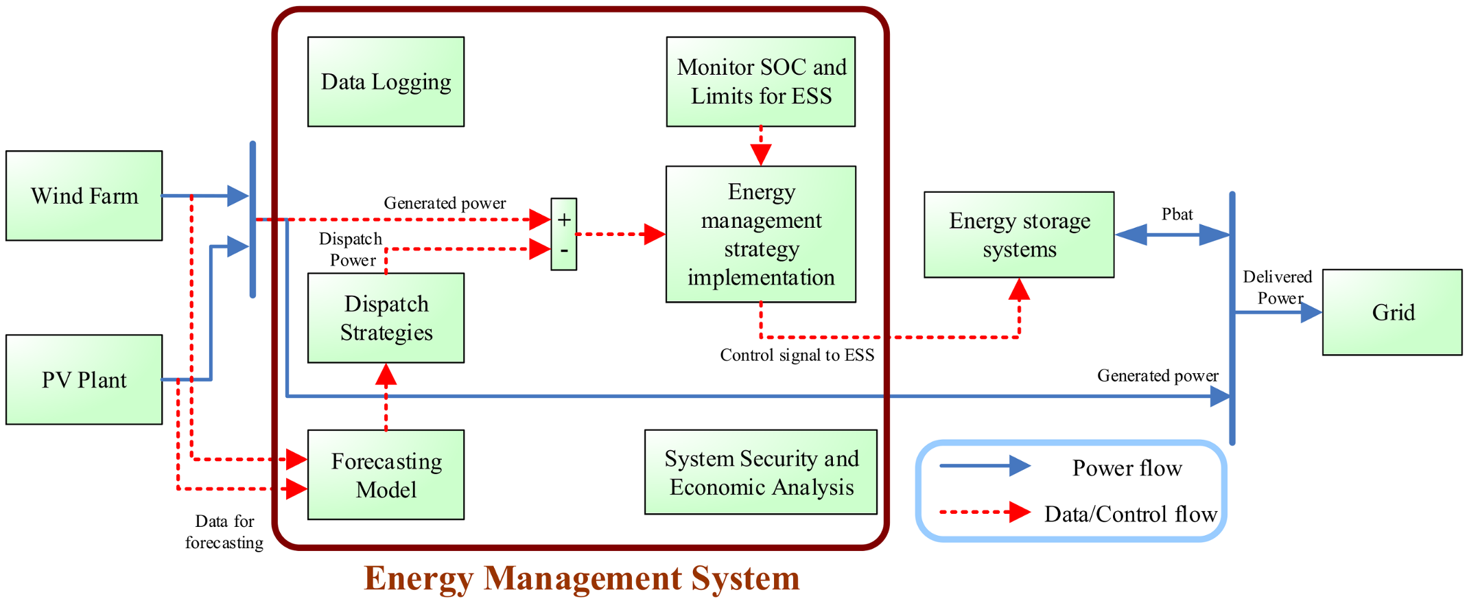
The architecture of the energy management scheme is illustrated in Figure 1. In Figure 1, the solid arrow denotes the power flow, and the dotted arrow denotes the data/control flow. It can be divided into three major parts. The first part on the left side of Figure 1 represents renewable energy generation (e.g., PV plant, wind farm, etc.). The second part represents the energy management system (EMS), which includes the output signal of the front-end prediction model for power dispatching, the battery state of charge (SOC), and the block that limits the energy storage system to the EMS. The second part is mainly composed of EMS and its control signal. If generated energy reaches the limit of the energy storage system, the remaining power can be fed to the grid.
The renewable sources act as a power system input, which the corresponding power system uses to generate the output power. On the other hand, the pyranometer and anemometer sensors detect the time series renewable source data and record it. Furthermore, according to the previous renewable source record, the forecasting model predicts the future solar radiation and wind speed. These forecasting results are then considered by the energy management system. The energy management system is a crucial part for the operation of the renewable power systems [31] because it handles all the renewable energy generating situations for an important power dispatching process. Therefore, precise forecasting of the future renewable source state is very important and necessary to predicting energy production and power dispatching. It has an important contribution to the power grid stability.
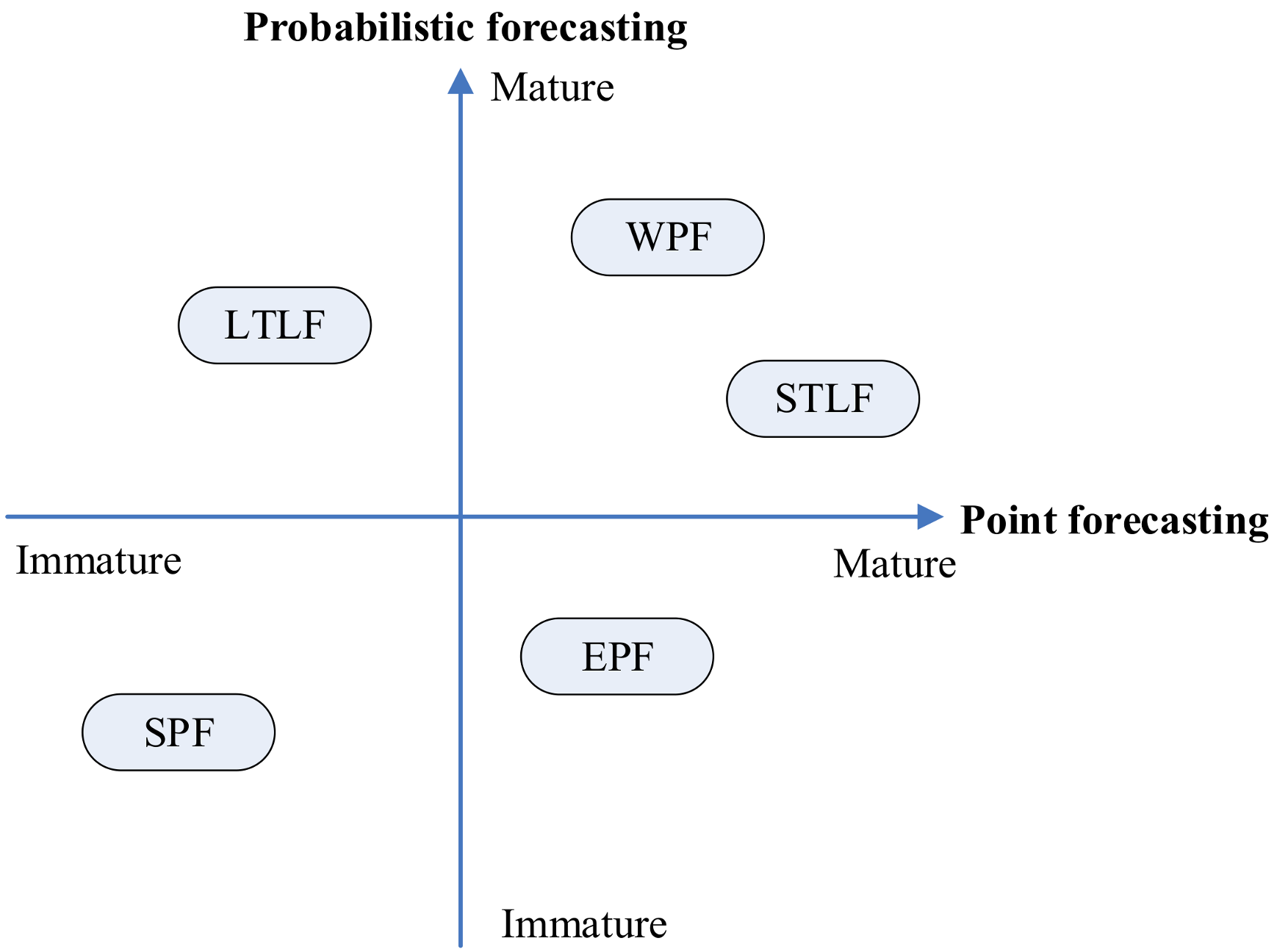
However, solar energy forecasting is still a big challenge. The maturity of energy forecasting is presented in Figure 2 [31,32], where the horizontal axis denotes the point forecasting (deterministic forecasting), and the vertical axis represents the probabilistic forecasting. The maturities of the related energy techniques—such as solar power forecasting (SPF), long term load forecasting (LTLF), electricity price forecasting (EPF), wind power forecasting (WPF), and short-term load forecasting (STLF)—are shown in Figure 2 [31,32]. Wind power forecasting occupies the highest position in the presented maturity diagram. Wind power forecasting is similar to weather forecasting, so its forecasting accuracy is as accurate as the one of weather forecasts. Up to now, due to the cloud move uncertainties and immature solar energy forecasting techniques, the difficulty level of SPF is much higher than of other forecasting techniques. However, the investigation of solar energy forecasting will flourish due to the increasing penetration of solar energy over the next decade [33]. In conclusion, the development of the SPF technique is absolutely important and urgent. Therefore, the goal of this study is to develop a high-precision solar forecasting model for the power dispatching process in the energy management system.
3. Neural Networks
In this section, several key concepts associated with the neural networks [35,36] are described, including 1D convolution, pooling layers, and dropout technology.
3.1. 1D Convolution
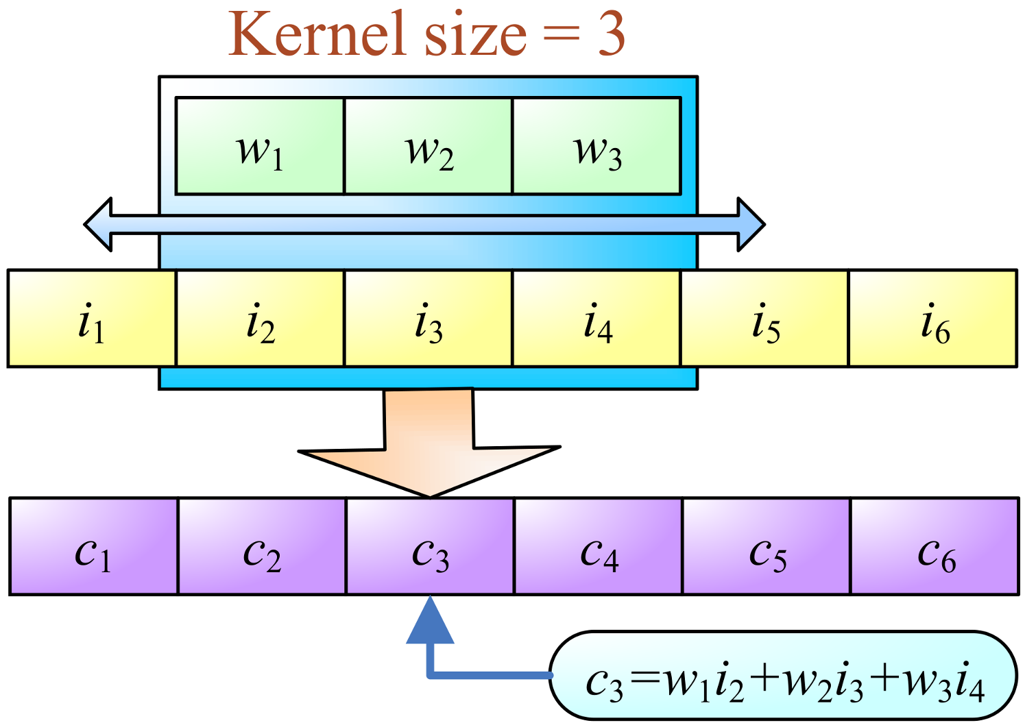
The convolutional neural network (CNN) is a powerful tool widely used in image classification. The CNNs use weight sharing, so they require fewer parameters than the conventional multilayer perceptron (MLP) networks, which makes CNNs converge far faster than the conventional neural network models. An example of calculations involved in a 1D convolution operation is presented in Figure 3. In this example, the kernel size is 3, which means that the weights (w1, w2, w3) are shared by every stride of the input layer (i1, i2, …, i6), and the output values are c1, c2, …, and c6. The input values in the kernel window are multiplied by the weights (w1, w2, w3). These values are then summarized and used as the feature map values. In the presented example, the feature c3 is obtained by c3 = w1 × i2+w2 × i3+w3 × i4.
3.2. Pooling Layer
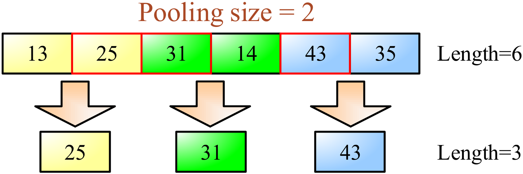
The pooling layer is crucial to the CNN. Pooling methods can be regarded as down-sampling operations aimed at reducing the number of parameters while retaining the most important features in order to speed up the next calculation step. The pooling operation is also meant to overcome the overfitting problem. Although numerous pooling methods can be used in CNNs, max pooling is the most common approach. The 1D max pooling operation is illustrated in Figure 4. The length of the feature map before pooling is 6, and the pooling size is 2. Therefore, the output value is reduced to 3, and the max values are selected as feature values for the next layer.
3.3. Dropout Technology
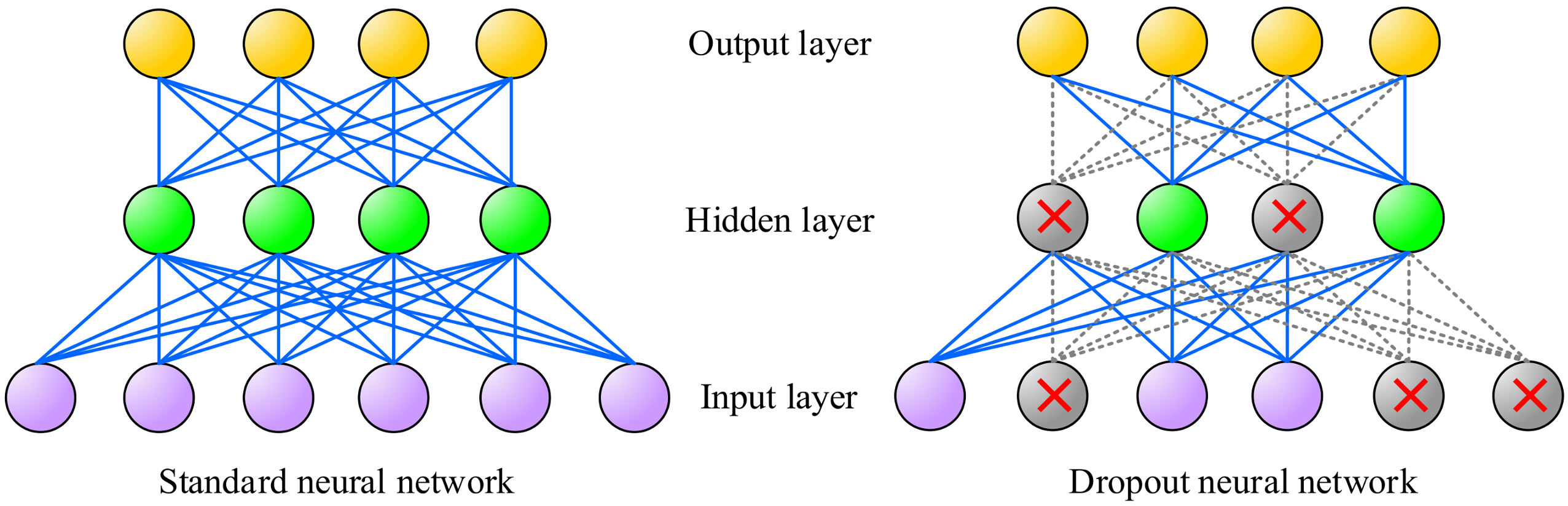
The serious overfitting problem during training can be mostly overcome using dropout technology [37]. Figure 5 presents two multilayered feedforward networks, i.e., a standard neural network (on the left) and a dropout neural network (on the right). The circles in Figure 5 denote the neurons, and the overlapping lines represent the weights. The bottom neurons denote the input layer, and the top neurons denote the output layer. All the input information is fed to the input layer and passed through the hidden layer (the middle neurons) to the output layer. The training of a neural network is performed by the backpropagation algorithm. During the training, the weights are tuned, and the neural network model is fitted according to the training data. The structure of the dropout neural network is almost the same.
The dropout neural network also consists of the input layer, hidden layer, and output layer. The dropout method involves the random selection of neurons and disabling of selected neurons during training such that the output values of randomly disabled neurons are zero. As shown on the right side of Figure 5, there are three disabled neurons in the first layer and two disabled neurons in the second layer, whose output values are temporarily set to zero. As indicated by the gray circles and dotted lines in Figure 5, the connections from disabled neurons are also temporarily removed. Even though some neurons are temporarily disabled, the neural network can still work well. Based on the simple random selection method of the “dead neurons,” the overfitting problem can be solved effectively [37].
4. Proposed SolarNet Structure
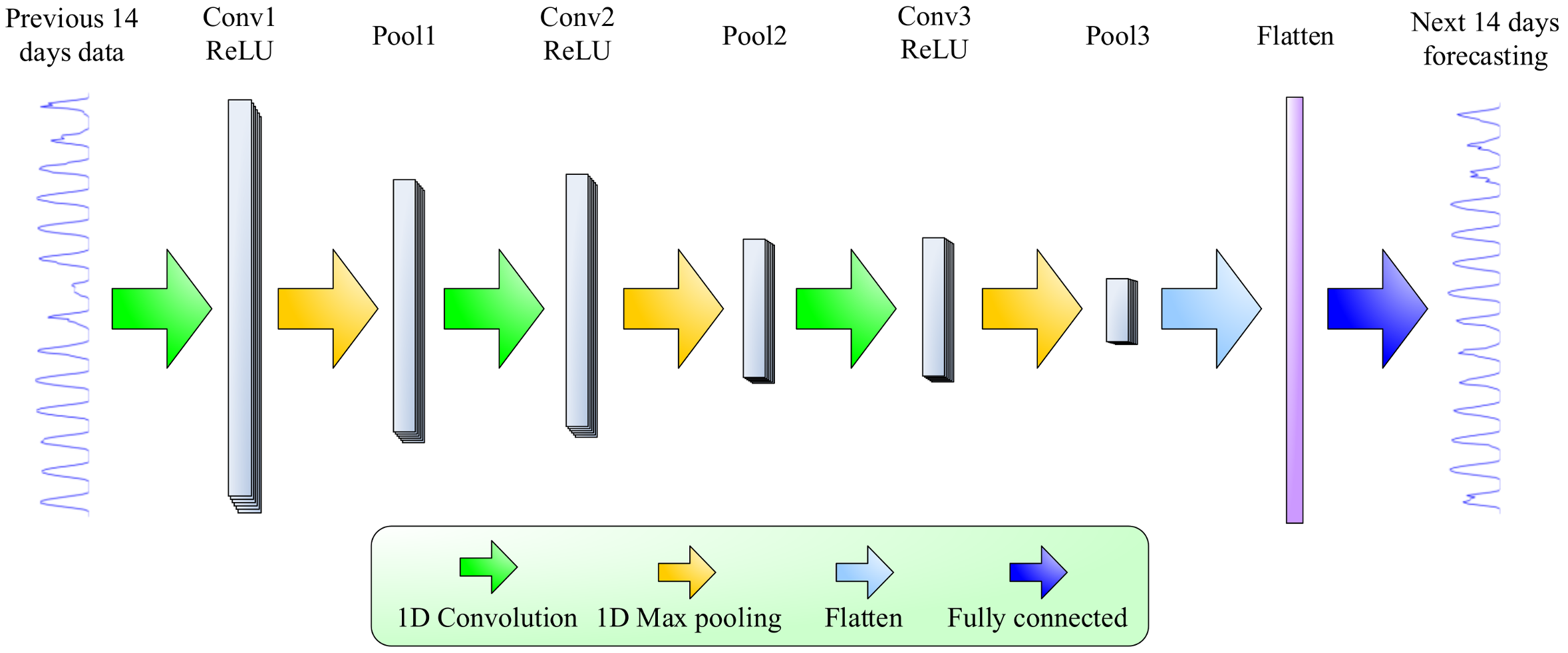
The proposed CNN-based SolarNet model is presented in Figure 6. The input data consist of solar radiation values over the previous 14 days, whereas the output values are the forecasting results over the next 14 days. The SolarNet includes three 1D convolution layers (Conv1, Conv2, and Conv3) and three pooling layers (Pool1, Pool2, and Pool3). The conventional activation function is a sigmoidal function defined by (1). However, the rectified linear unit (ReLU) is employed here as an activation function of the convolution and output layers to reduce the chance of gradient vanishing. The ReLU function is described by (2).
The number of filters in Conv1, Conv2, and Conv3 is 16, 32, and 64, respectively, which means that the “thickness” of Conv1, Conv2, and Conv3 is 16, 32, and 64, respectively. We set the kernel sizes of Conv1, Conv2, and Conv3 to 9, 5, and 5, respectively. The pooling size of each pooling layer is 2, and the “length” of the feature map is reduced by pooling operations. After processing using three convolution layers and three pooling layers, the feature map of Pool3 is flattened into a 1D feature map denoting the final feature extraction result. The last layer of the SolarNet model is fully connected. To prevent overfitting during training, we apply the dropout technique to the flatten layer with the dropout rate of 0.15. During the training process, the order of the training data is shuffled between each epoch, and the batch size is set to 32. The final output is the forecasting results for the next 14 days.
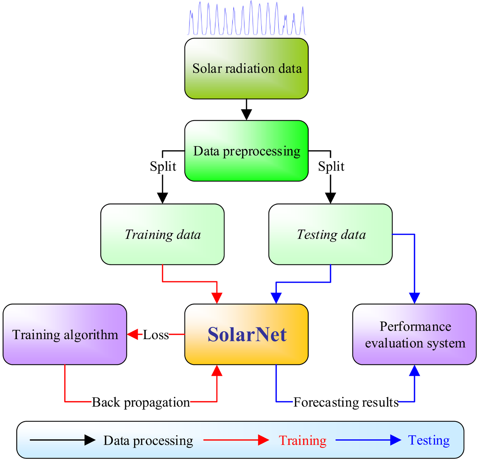
The architecture of the solar radiation forecasting system including three types of processes is illustrated in Figure 7. The black arrows in Figure 7 indicate data processing, the red arrows indicate the training processes, and the blue arrows indicate the testing processes. First of all, the solar radiation data are preprocessed (i.e., scaled to [0, 1]) and then split into the training dataset and testing dataset. Training data are used for training of the SolarNet model which represents the weights updated using the backpropagation algorithm. After training, the testing data is fed to the SolarNet to obtain forecasting results. The forecasting performance of the proposed system is determined by comparing these forecasting results with the ground truth of testing data.
The input data of the proposed CNN model are the information on solar radiation over previous 14 days, and the output data of the model are the information on solar radiation over the next 14 days. As shown in Figure 7, the data are separated into training data and testing data. The training data are used for model training, and the testing data are utilized for the evaluation of the model performance. The training data includes a large number of training pairs consisting of input data and the corresponding output data. Hence, every pair has information on solar radiation over a period of 28 days, where the first 14 days are used as a CNN model input, and the next 14 days are used to define the desired output. As already mentioned, the training pairs are used to train the CNN model to fit the given input and output data by adjusting the weights’ values. After the training process, the model can predict the solar radiation level over the next 14 days. Also, after the training process, if the training data are fed to the model, the model gives the forecasting result with almost zero error. However, solar radiation in the practice is unknown and can differ from the training data. Therefore, the testing data, which has not been included in the model training, are used to evaluate model performance, i.e., the generalization ability. The structure of the testing data is the same as that of the training data. Namely, the testing data also consists of data pairs where every pair has the information on the solar radiation levels over 28 days. The data over the first 14 days are used as input data and the data over the last 14 days are used as output data. The forecasting result is compared to the ground truth data (i.e., the solar radiation in the next 14 days) to evaluate model performance.
5. Experimental Results
In this section, the test results are described in detail. The test results also include the comparison of the SolarNet performance with the performances of a Support Vector Machine (SVM) [38], Random Forest (RF) [39], Decision Tree (DT) [40], Multilayer Perceptron (MLP) [41], and Long Short Term Memory (LSTM) networks [42].
5.1. Data Description
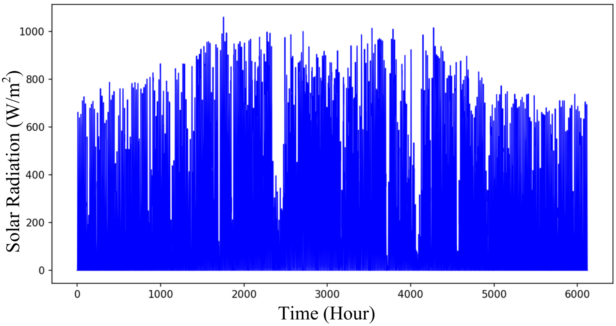
The data contained samples of solar radiance. These samples define the resolution of the radiometer, which determines the predictability of the dataset. The solar radiation data were collected by computer monitoring system of the PV sites in Tainan. We employed a radiometer (ISO 9060 Class 2) to capture at least one data record per minute and A/D signal converter to enable network storage to the gateway. The data were sent on a daily basis via the Internet using the Internet File Transfer Protocol (FTP) protocol from the network gateway to the back-end servers. The solar radiation dataset for Tainan (Taiwan) in 2015 is presented in Figure 8. As shown in Figure 8, the weather characteristic in Tainan (i.e., high uncertainty of the solar radiation) may still influence the forecasting results.
5.2. Comparison Results
To obtain better insight into the proposed model performance, we compared its performances with the performances of commonly used forecasting models. The mean absolute error (MAE) was used to evaluate and compare the performances of SVM, random forest, decision tree, MLP, LSTM, and the proposed SolarNet model. The value of MAE was calculated using Equation (3), where yn denotes the measured value, denotes the estimated value, and N denotes the number of samples.
The PV system instability impacts on the access to the grid, so it needs to predict PV power output on the grid. Also, under the influence of many factors such as weather, clouds, humidity, and season, the PV system shows very complicated nonlinear characteristics and it is difficult to predict solar radiation intensity accurately. Moreover, the longer the forecast period is, the greater the forecast error will be. The amount of solar radiation has the greatest impact on the PV system. Therefore, this paper presents a medium-term forecasting method commonly used in deep learning and analyzes the theoretical basis and characteristics of different prediction methods.
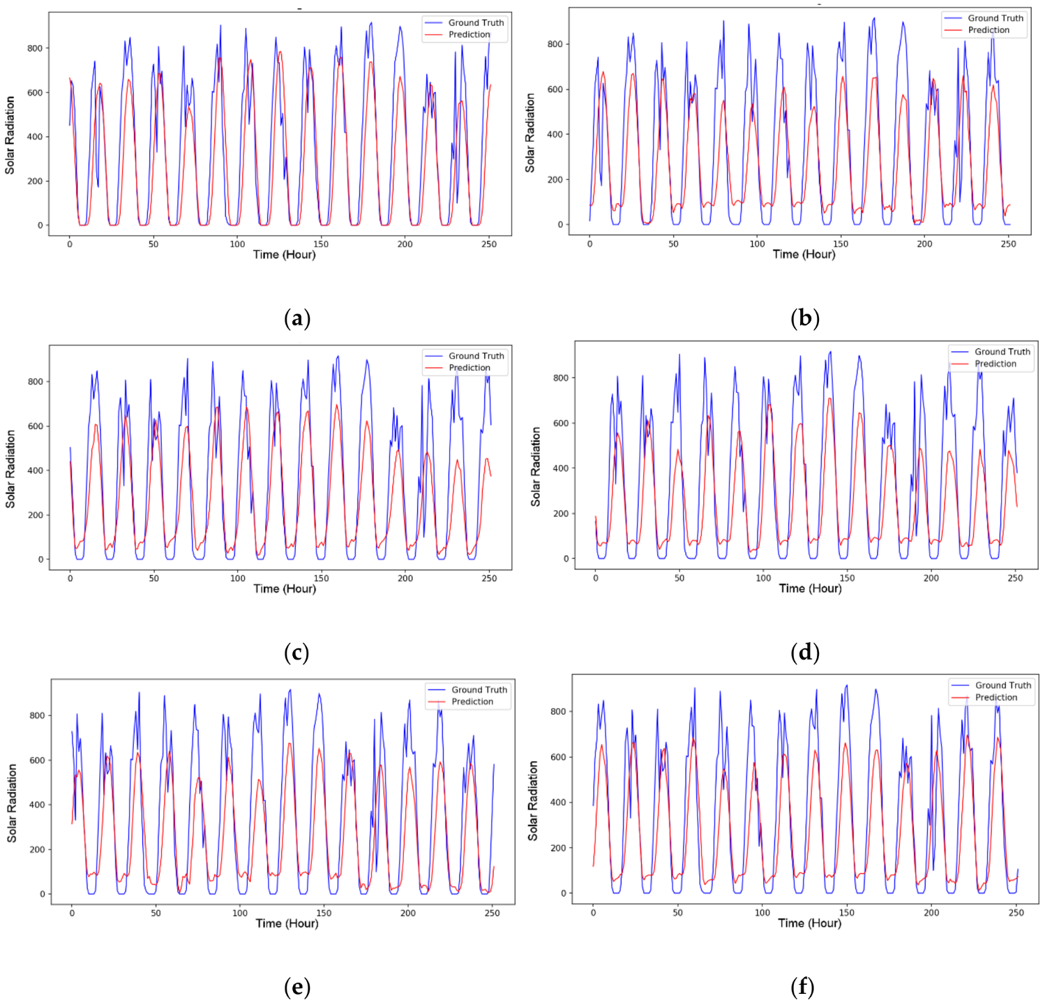
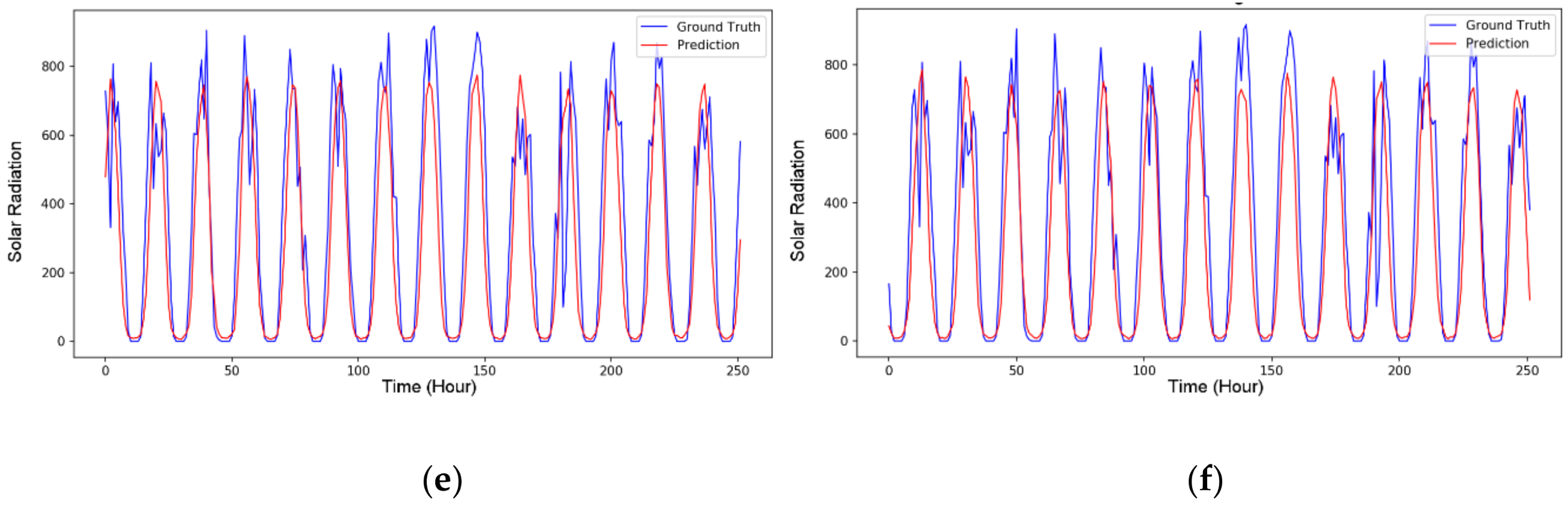
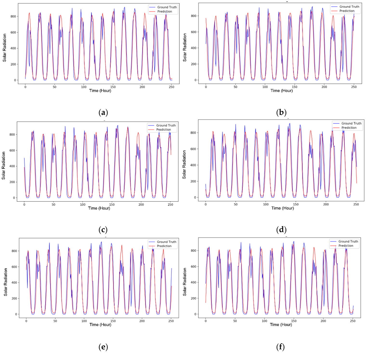
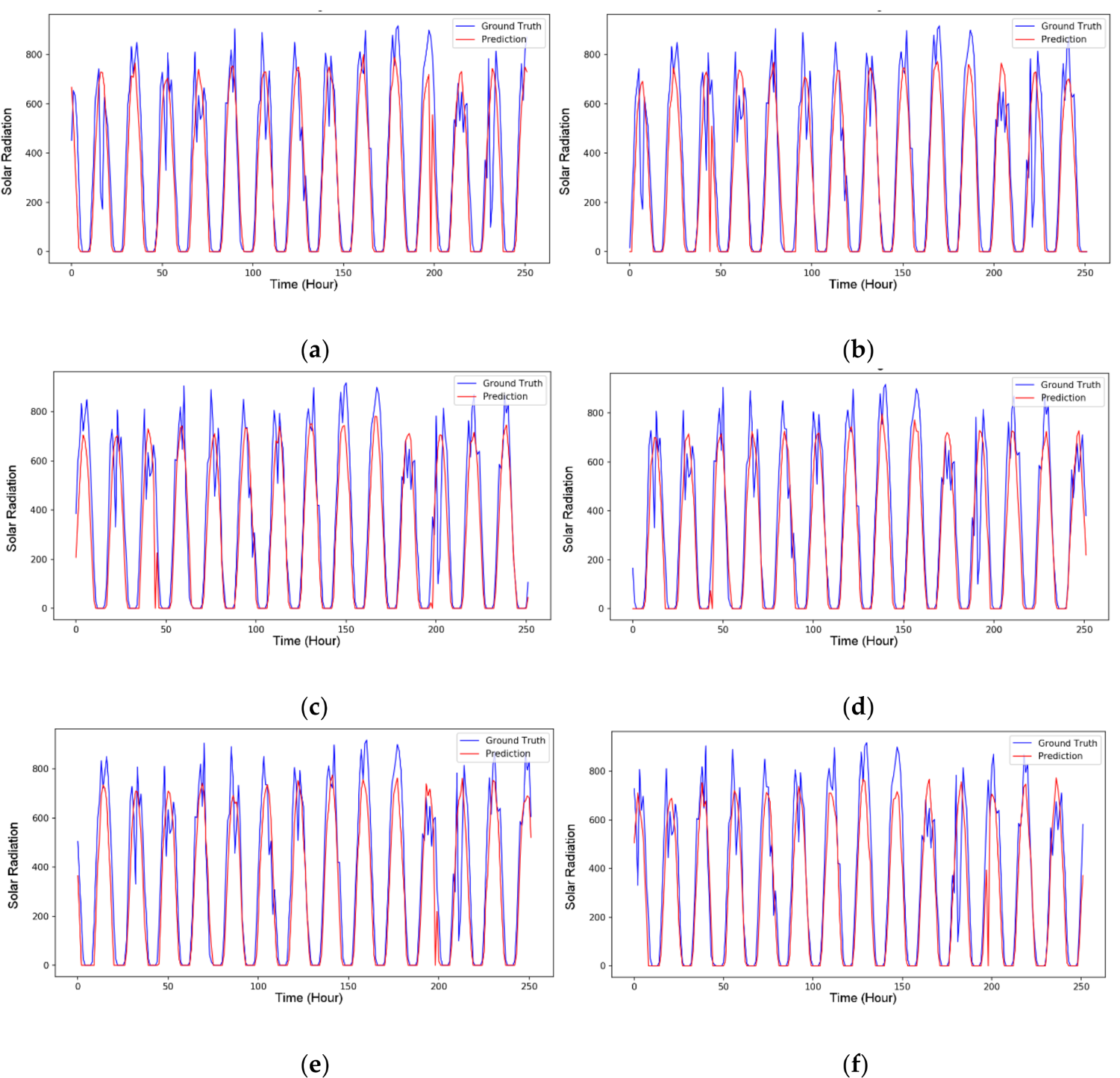
The results are presented in Figure 9, Figure 10, Figure 11, Figure 12, Figure 13 and Figure 14, wherein it can be seen that the proposed forecasting model can deal with the nonlinear problems well and provides much better results in solar radiation forecasting than the other tested methods. The training data covered a period of four months, and the testing data covered a period of two months. We conducted 11 tests to obtain a comprehensive evaluation of the performances of all tested methods. In the first test, the training data includes the solar radiation data in the first four months, and the testing data covers the solar radiation data in the fifth and sixth months. With respect to the second test, the selected range of training and testing data are all shifted forward by half a month from the range of the first test. The rest of the data is shifted along the same line of reasoning. Furthermore, the solar radiation dataset included data obtained over the period of one year (2015). According to the climate characteristics of Taiwan, there are generally four distinct seasons in Taiwan. Therefore, based on different seasonal conditions, the measured data from one year can almost cover all the possible scenarios regarding solar radiation fluctuations. In this experiment, all the training data and testing data are obtained from actual numbers, and there are no simulated data included in the tests.
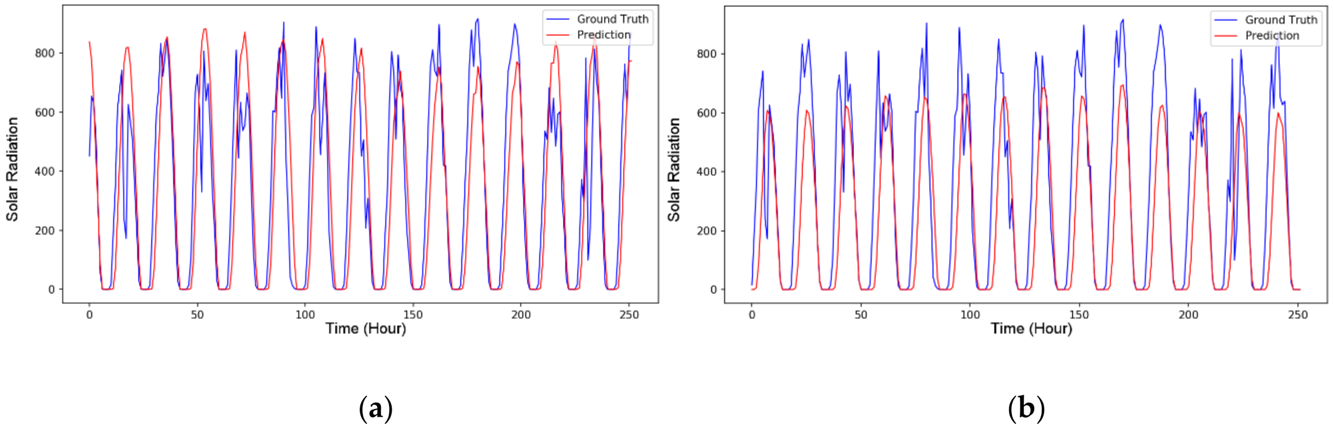
The comparison of the machine learning algorithms regarding the MAE values is presented numerically in Table 1. Every method was subjected to every test using the testing data covering a period of two months. As shown in Table 1, the SolarNet outperformed all other algorithms in tests 2, 4, 5, 8, 9, 10, and 11, and it obtained the lowest average MAE value. The test results show that the random forest and LSTM methods achieved good results. However, even they failed to reach the performance of the SolarNet.
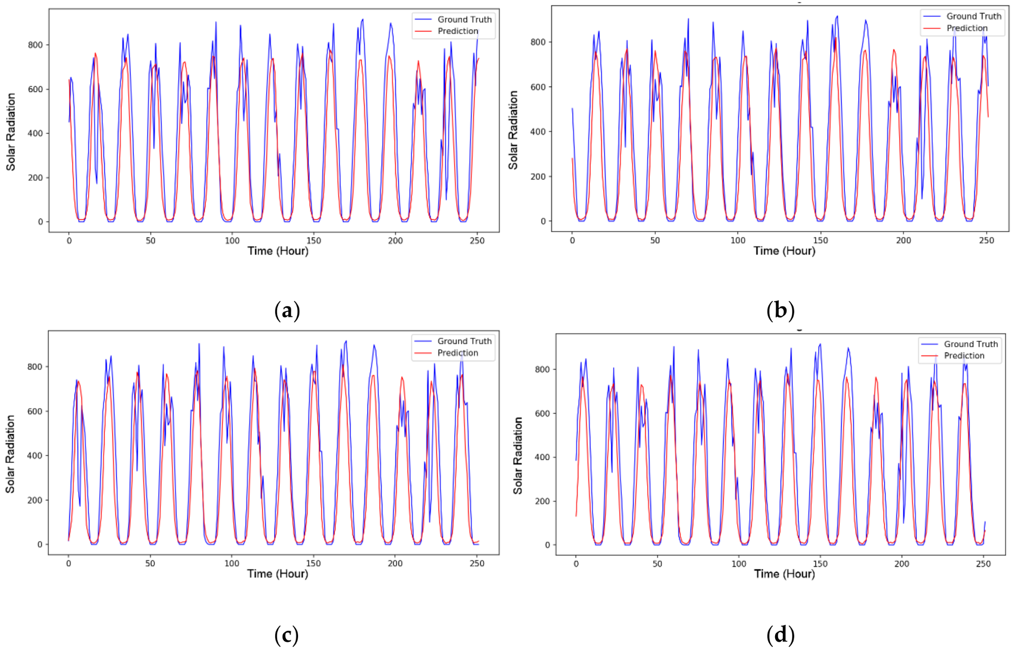
As already mentioned, the solar radiation over the past 336 h (24 h × 14 days) was used as an input of the forecasting model, and the predicted solar radiation over the next 336 h (24 h × 14 days) was an output of the forecasting model. The SolarNet achieved the lowest MAE (average of 112.264) and the best goodness of error among all models. The decision tree (DT) model achieved the highest MAE with an average error of 143.2721. Based on the average MAE values, the forecasting accuracy in descending order was as follows: SolarNet, RF, LSTM, MLP, SVM, and DT. The concept of random forest (RF) is to use many DTs to decide the regression results. The RF is also one of the model ensemble methods. The results show that the model based on the ensemble method is effective in solar radiation forecasting. On the other hand, the LSTM represents one of the recurrent neural network models, and it considers the time sequence relationship of the input data. The LSTM achieved an acceptable result in the tests, showing that the recurrent neural network model can handle solar radiation forecasting. However, the MAE values of MLP, SVM, and DT are higher than those of SolarNet, RF, and LSTM. Consequently, it can be concluded that these three traditional machine learning methods (MLP, SVM, and DT) still cannot handle the complex time series forecasting with a high degree of volatility and irregularity.
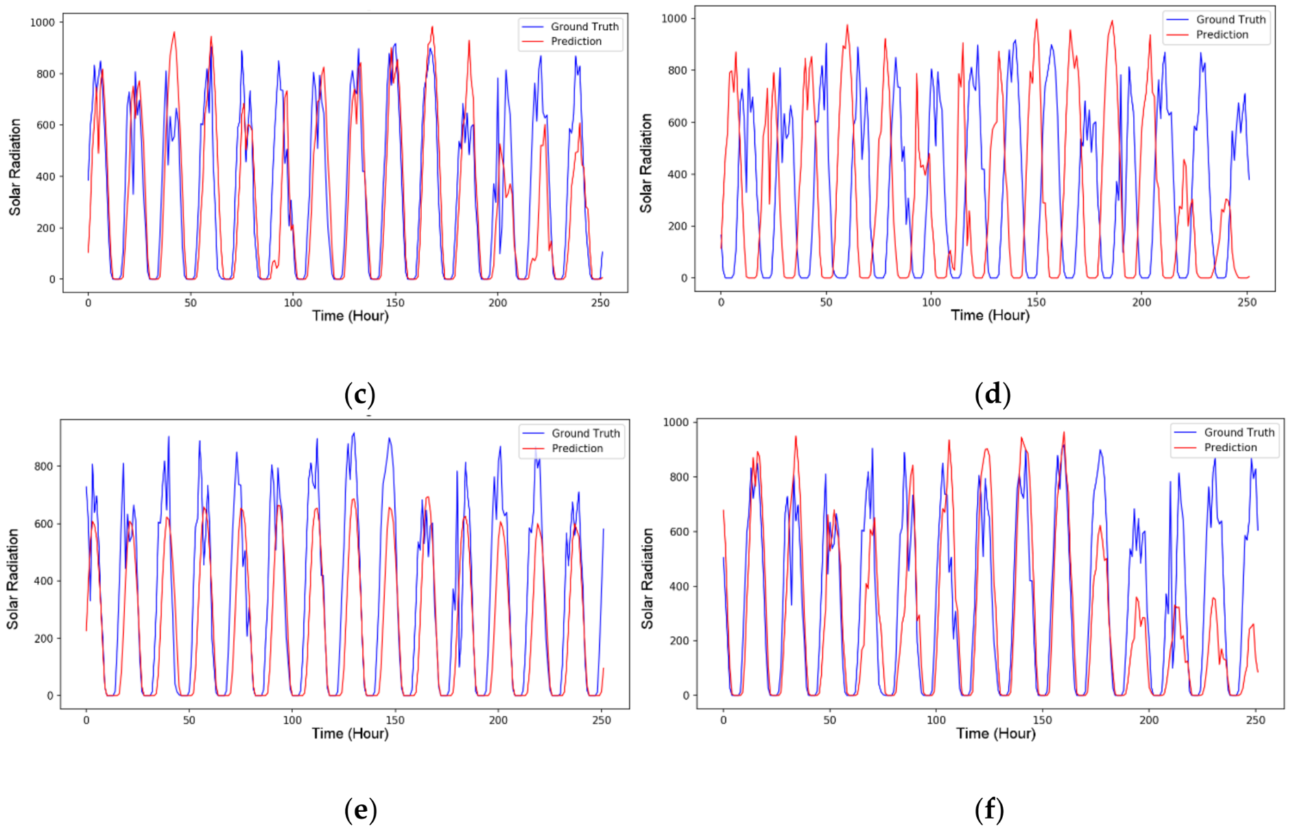
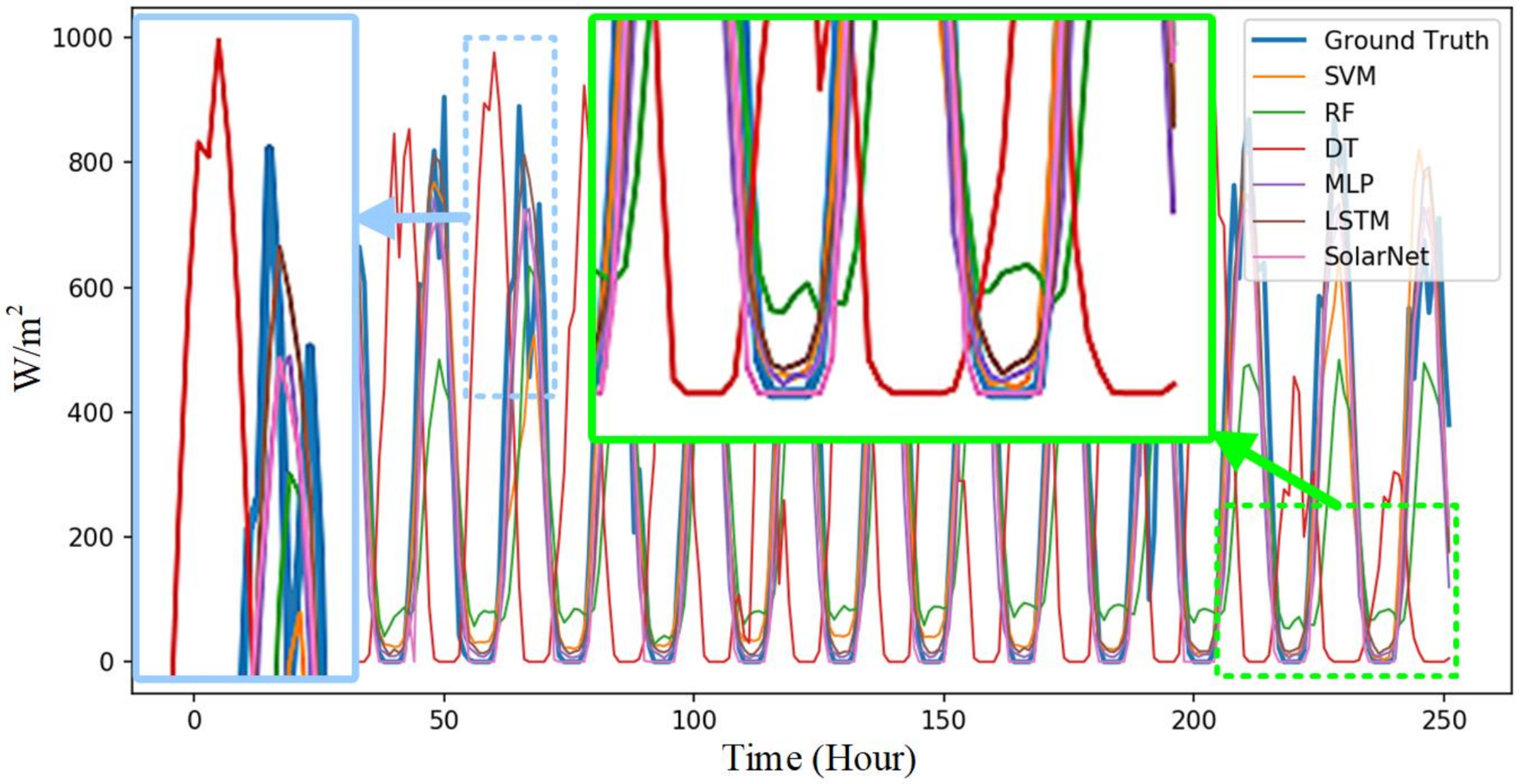
The graphical comparison of forecasting results is presented in Figure 15, where the blue rectangle shows the forecasting results in the peak area. The forecasting result of the decision tree is denoted by a red curve. As seen in Figure 15, the difference between the ground truth and the decision tree forecasting result is very large, which shows that a decision tree is not capable of handling the solar forecasting. Even though the SVM and random forest provided better results, the forecasting results in the peak areas are still unsatisfactory. On the other hand, the MLP, LSTM, and the proposed SolarNet provided good performances. Namely, the trend of solar radiation was comprehensively learned and forecasted by these three models.
The green rectangle in Figure 15 shows the forecasting results in the bottom area. In this case, the forecasting results of the decision tree and random forest are still not good enough. Compared to the other models, the forecasting error of the decision tree and random forest is too large, which may cause the misjudgments during power dispatching. However, the pink curve, which denotes the forecasting result of the SolarNet, is very fitting to the ground truth. The results show that the proposed SolarNet has the ability to provide good forecasting performance, and the MAE of SolarNet is the smallest one. Therefore, the feasibility of the proposed SolarNet model for an energy management system is verified.
6. Conclusions
This paper presents a high-precision deep convolutional neural network model, called the SolarNet, intended for solar radiation forecasting. The developed model uses the latest deep learning technology to solve the important solar forecasting problem and improve the prediction accuracy. The SolarNet uses the data over the previous 14 days collected from a pyranometer sensor to forecast the solar radiation over the next 14 days with a very low MAE. The performance of the SolarNet in solar radiation forecasting was validated and compared with the performances of SVM, RF, DT, MLP, and LSTM. The SolarNet achieved good results in tests and demonstrated that it is feasible for highly-accurate forecasting. The comparison results verified that, in medium-term forecasting, the SolarNet forecasting model has good generalizability and robustness in providing high accuracy. This study not only validates that the CNN model is effective and practical but also creates a new research direction in the forecasting field.
Acknowledgments
This work was supported by the Ministry of Science and Technology, Taiwan, China, under Grants MOST 106-2218-E-153-001-MY3.
Author Contributions
Ping-Huan Kuo wrote the program and designed the solar radiation forecasting model. Chiou-Jye Huang planned this study and collected the solar radiation dataset. Ping-Huan Kuo and Chiou-Jye Huang contributed to the realization and revision of the manuscript.
Conflicts of Interest
The authors declare no conflict of interest.
References
- Renewable, I.; Agency, E. Renewable Capacity Statistics 2016 Statistiques; IRENA (International Renewable Energy Agency): Masdar City, United Arab Emirates, 2016; ISBN 9789295111905. [Google Scholar]
- Yang, D. Solar Irradiance Modeling and Forecasting Using Novel Statistical Techniques. Ph.D. Thesis, National University of Singapore, Singapore, Singapore, 2014. [Google Scholar]
- Wei, C.-C. Predictions of Surface Solar Radiation on Tilted Solar Panels using Machine Learning Models: A Case Study of Tainan City, Taiwan. Energies 2017, 10, 1660. [Google Scholar] [CrossRef]
- Kardakos, E.G.; Alexiadis, M.C.; Vagropoulos, S.I.; Simoglou, C.K.; Biskas, P.N.; Bakirtzis, A.G. Application of time series and artificial neural network models in short-term forecasting of PV power generation. In Proceedings of the 2013 48th International Universities’ Power Engineering Conference (UPEC), Dublin, Ireland, 2–5 September 2013. [Google Scholar] [CrossRef]
- Trapero, J.R.; Kourentzes, N.; Martin, A. Short-term solar irradiation forecasting based on dynamic harmonic regression. Energy 2015, 84, 289–295. [Google Scholar] [CrossRef] [Green Version]
- Huang, J.; Korolkiewicz, M.; Agrawal, M.; Boland, J. Forecasting solar radiation on an hourly time scale using a Coupled AutoRegressive and Dynamical System (CARDS) model. Sol. Energy 2013, 87, 136–149. [Google Scholar] [CrossRef]
- Voyant, C.; Paoli, C.; Muselli, M.; Nivet, M. Multi-horizon solar radiation forecasting for Mediterranean locations using time series models. Renew. Sustain. Energy Rev. 2013, 28, 44–52. [Google Scholar] [CrossRef]
- Hu, W.; Yang, C. Grey model of direct solar radiation intensity on the horizontal plane for cooling loads calculation. Build. Environ. 2000, 35, 587–593. [Google Scholar] [CrossRef]
- Chen, S.X.; Gooi, H.B.; Wang, M.Q. Solar radiation forecast based on fuzzy logic and neural networks. Renew. Energy 2013, 60, 195–201. [Google Scholar] [CrossRef]
- Mellit, A. APPLIED An adaptive wavelet-network model for forecasting daily total solar-radiation. Appl. Energy 2006, 83, 705–722. [Google Scholar] [CrossRef]
- Deo, R.C.; Wen, X.; Qi, F. A wavelet-coupled support vector machine model for forecasting global incident solar radiation using limited meteorological dataset. Appl. Energy 2016, 168, 568–593. [Google Scholar] [CrossRef]
- Cao, J.C.; Cao, S.H. Study of forecasting solar irradiance using neural networks with preprocessing sample data by wavelet analysis. Energy 2006, 31, 3435–3445. [Google Scholar] [CrossRef]
- Capizzi, G.; Napoli, C.; Bonanno, F. Innovative Second-Generation Wavelets Construction with Recurrent Neural Networks for Solar Radiation Forecasting. IEEE Trans. Neural Netw. Learn. Syst. 2012, 23, 1805–1815. [Google Scholar] [CrossRef] [PubMed]
- Hassan, S.; Khanesar, M.A.; Hajizadeh, A.; Khosravi, A. Hybrid multi-objective forecasting of solar photovoltaic output using Kalman filter based interval type-2 fuzzy logic system. IEEE Int. Conf. Fuzzy Syst. 2017. [Google Scholar] [CrossRef]
- Soubdhan, T.; Ndong, J.; Ould-Baba, H.; Do, M.T. A robust forecasting framework based on the Kalman filtering approach with a twofold parameter tuning procedure: Application to solar and photovoltaic prediction. Sol. Energy 2016, 131, 246–259. [Google Scholar] [CrossRef]
- Cheng, H.Y. Hybrid solar irradiance now-casting by fusing Kalman filter and regressor. Renew. Energy 2016, 91, 434–441. [Google Scholar] [CrossRef]
- Mathiesen, P.; Kleissl, J. Evaluation of numerical weather prediction for intra-day solar forecasting in the continental United States. Sol. Energy 2011, 85, 967–977. [Google Scholar] [CrossRef]
- Mellit, A.; Massi, A. A 24-h forecast of solar irradiance using artificial neural network: Application for performance prediction of a grid-connected PV plant at Trieste, Italy. Sol. Energy 2010, 84, 807–821. [Google Scholar] [CrossRef]
- Benmouiza, K.; Cheknane, A. Forecasting hourly global solar radiation using hybrid k-means and nonlinear autoregressive neural network models. Energy Convers. Manag. 2013, 75, 561–569. [Google Scholar] [CrossRef]
- Bae, K.Y.; Jang, H.S.; Sung, D.K. Hourly Solar Irradiance Prediction Based on Support Vector Machine and Its Error Analysis. IEEE Trans. Power Syst. 2016, 32, 935–945. [Google Scholar] [CrossRef]
- Olatomiwa, L.; Mekhilef, S.; Shamshirband, S.; Mohammadi, K.; Petković, D.; Sudheer, C. A support vector machine-firefly algorithm-based model for global solar radiation prediction. Sol. Energy 2015, 115, 632–644. [Google Scholar] [CrossRef]
- Niu, D.; Dai, S. A Short-Term Load Forecasting Model with a Modified Particle Swarm Optimization Algorithm and Least Squares Support Vector Machine Based on the Denoising Method of Empirical Mode Decomposition and Grey Relational Analysis. Energies 2017, 10, 408. [Google Scholar] [CrossRef]
- Voyant, C.; Notton, G.; Kalogirou, S.; Nivet, M.; Paoli, C.; Motte, F.; Fouilloy, A. Machine learning methods for solar radiation forecasting: A review. Renew. Energy 2017, 105, 569–582. [Google Scholar] [CrossRef]
- Lauret, P.; Voyant, C.; Soubdhan, T.; David, M.; Poggi, P. ScienceDirect A benchmarking of machine learning techniques for solar radiation forecasting in an insular context. Sol. Energy 2015, 112, 446–457. [Google Scholar] [CrossRef]
- Li, J.; Ward, J.K.; Tong, J.; Collins, L.; Platt, G. Machine learning for solar irradiance forecasting of photovoltaic system. Renew. Energy 2016, 90, 542–553. [Google Scholar] [CrossRef]
- Diagne, M.; David, M.; Lauret, P.; Boland, J.; Schmutz, N. Review of solar irradiance forecasting methods and a proposition for small-scale insular grids. Renew. Sustain. Energy Rev. 2013, 27, 65–76. [Google Scholar] [CrossRef]
- Law, E.W.; Prasad, A.A.; Kay, M.; Taylor, R.A. ScienceDirect Direct normal irradiance forecasting and its application to concentrated solar thermal output forecasting—A review Australia Bureau of Meteorology. Sol. Energy 2014, 108, 287–307. [Google Scholar] [CrossRef]
- Photovoltaic Power Forecasting System SPSF-3000. Available online: http://www.sprixin.com/product/product_detail-2.htm (accessed on 25 March 2018).
- Lv, Y.; Guan, L.; Tang, Z.; Zhao, Q. A Probability Model of PV for the Middle-term to Long-term Power System Analysis and Its Application. Energy Procedia 2016, 103, 28–33. [Google Scholar] [CrossRef]
- Alanazi, M.S. Solar Power Deployment: Forecasting and Planning. Ph.D. Thesis, University of Denver, Denver, CO, USA, 2014. [Google Scholar]
- Gharavi, H.; Ardehali, M.M.; Ghanbari-tichi, S. Imperial competitive algorithm optimization of fuzzy multi-objective design of a hybrid green power system with considerations for economics, reliability and environmental emissions. Renew. Energy 2015, 78, 427–437. [Google Scholar] [CrossRef]
- Fathima, H.; Palanisamy, K. Energy Storage Systems for Energy Management of Renewables in Distributed Generation Systems. In Energy Management of Distributed Generation Systems; InTech: London, UK, 2016. [Google Scholar]
- Hong, T.; Pinson, P.; Fan, S.; Zareipour, H.; Troccoli, A.; Hyndman, R.J. Probabilistic energy forecasting : Global Energy Forecasting Competition 2014 and beyond. Int. J. Forecast. 2016, 32, 896–913. [Google Scholar] [CrossRef] [Green Version]
- Antonanzas, J.; Osorio, N.; Escobar, R.; Urraca, R.; Martinez-de-pison, F.J.; Antonanzas-torres, F. Review of photovoltaic power forecasting. Sol. Energy 2016, 136, 78–111. [Google Scholar] [CrossRef]
- Hernández, L.; Baladrón, C.; Aguiar, J.M.; Calavia, L.; Carro, B.; Sánchez-Esguevillas, A.; García, P.; Lloret, J. Experimental analysis of the input variables’ relevance to forecast next day’s aggregated electric demand using neural networks. Energies 2013, 6, 2927–2948. [Google Scholar] [CrossRef]
- Hernández, L.; Baladrón, C.; Aguiar, J.M.; Calavia, L.; Carro, B.; Sánchez-Esguevillas, A.; Sanjuán, J.; González, Á.; Lloret, J. Improved short-term load forecasting based on two-stage predictions with artificial neural networks in a microgrid environment. Energies 2013, 6, 4489–4507. [Google Scholar] [CrossRef]
- Srivastava, N.; Hinton, G.; Krizhevsky, A.; Sutskever, I.; Salakhutdinov, R. Dropout: A Simple Way to Prevent Neural Networks from Overfitting. J. Mach. Learn. Res. 2014, 15, 1929–1958. [Google Scholar] [CrossRef]
- Suykens, J.A.K.; Vandewalle, J. Least squares support vector machine classifiers. Neural Process. Lett. 1999, 9, 293–300. [Google Scholar] [CrossRef]
- Liaw, A.; Wiener, M. Classification and Regression by randomForest. R News 2002, 2, 18–22. [Google Scholar] [CrossRef]
- Safavian, S.R.; Landgrebe, D. A Survey of Decision Tree Classifier Methodology. IEEE Trans. Syst. Man Cybern. 1991, 21, 660–674. [Google Scholar] [CrossRef]
- White, B.W.; Rosenblatt, F. Principles of Neurodynamics: Perceptrons and the Theory of Brain Mechanisms. Am. J. Psychol. 1963, 76, 705. [Google Scholar] [CrossRef]
- Hochreiter, S.; Urgen Schmidhuber, J. Long Short-Term Memory. Neural Comput. 1997, 9, 1735–1780. [Google Scholar] [CrossRef] [PubMed]
Figure 1.
The architecture of the energy management scheme [32].
Figure 1.
The architecture of the energy management scheme [32].


Figure 3.
Calculations involved in a 1D convolution operation.

Figure 4.
1D max pooling operation.

Figure 5.
An illustration of standard and dropout neural networks.

Figure 6.
The structure of the proposed SolarNet model.

Figure 7.
The architecture of solar radiation forecasting system.

Figure 8.
The solar radiation dataset for Tainan (Taiwan) in 2015.

Figure 9.
Forecasting results of support vector machine: (a) Partial results A; (b) Partial results B; (c) Partial results C; (d) Partial results D; (e) Partial results E; (f) Partial results F.
Figure 9.
Forecasting results of support vector machine: (a) Partial results A; (b) Partial results B; (c) Partial results C; (d) Partial results D; (e) Partial results E; (f) Partial results F.

Figure 10.
Forecasting results of random forest: (a) Partial results A; (b) Partial results B; (c) Partial results C; (d) Partial results D; (e) Partial results E; (f) Partial results F.
Figure 10.
Forecasting results of random forest: (a) Partial results A; (b) Partial results B; (c) Partial results C; (d) Partial results D; (e) Partial results E; (f) Partial results F.

Figure 11.
Forecasting results of decision tree: (a) Partial results A; (b) Partial results B; (c) Partial results C; (d) Partial results D; (e) Partial results E; (f) Partial results F.
Figure 11.
Forecasting results of decision tree: (a) Partial results A; (b) Partial results B; (c) Partial results C; (d) Partial results D; (e) Partial results E; (f) Partial results F.


Figure 12.
Forecasting results of multilayer perceptron: (a) Partial results A; (b) Partial results B; (c) Partial results C; (d) Partial results D; (e) Partial results E; (f) Partial results F.
Figure 12.
Forecasting results of multilayer perceptron: (a) Partial results A; (b) Partial results B; (c) Partial results C; (d) Partial results D; (e) Partial results E; (f) Partial results F.


Figure 13.
Forecasting results of long short term memory network: (a) Partial results A; (b) Partial results B; (c) Partial results C; (d) Partial results D; (e) Partial results E; (f) Partial results F.
Figure 13.
Forecasting results of long short term memory network: (a) Partial results A; (b) Partial results B; (c) Partial results C; (d) Partial results D; (e) Partial results E; (f) Partial results F.

Figure 14.
Forecasting results of the proposed SolarNet: (a) Partial results A; (b) Partial results B; (c) Partial results C; (d) Partial results D; (e) Partial results E; (f) Partial results F.
Figure 14.
Forecasting results of the proposed SolarNet: (a) Partial results A; (b) Partial results B; (c) Partial results C; (d) Partial results D; (e) Partial results E; (f) Partial results F.

Figure 15.
Comparison of forecasting results.


Table 1.
Experimental results in terms of Mean Absolute Error (MAE).
| Test | Support Vector Machine (SVM) | Random Forest (RF) | Decision Tree (DT) | Multilayer Perceptron (MLP) | Long Short Term Memory (LSTM) | SolarNet |
|---|---|---|---|---|---|---|
| #1 | 140.2472 | 120.8082 | 147.1849 | 134.647 | 122.829 | 125.949 |
| #2 | 108.7249 | 129.3671 | 156.0479 | 116.662 | 107.255 | 104.035 |
| #3 | 133.4374 | 133.7141 | 172.3512 | 117.441 | 115.831 | 134.09 |
| #4 | 134.8683 | 129.2832 | 158.2685 | 116.976 | 117.839 | 112.52 |
| #5 | 164.1875 | 134.1216 | 144.1382 | 145.416 | 145.299 | 132.296 |
| #6 | 181.2317 | 133.1271 | 142.6717 | 172.1990 | 159.5790 | 145.6360 |
| #7 | 166.3924 | 129.9551 | 143.7967 | 161.8980 | 148.485 | 131.1760 |
| #8 | 133.8187 | 119.0586 | 149.4838 | 131.8890 | 132.049 | 110.4330 |
| #9 | 100.9875 | 88.65956 | 123.2007 | 111.4450 | 100.441 | 77.9005 |
| #10 | 102.4227 | 106.0825 | 125.0525 | 105.8540 | 90.789 | 77.7337 |
| #11 | 119.3462 | 104.1780 | 113.7968 | 99.9288 | 93.7216 | 83.1351 |
| Average | 135.0604 | 120.7595 | 143.2721 | 128.5778 | 121.2830 | 112.2640 |
© 2018 by the authors. Licensee MDPI, Basel, Switzerland. This article is an open access article distributed under the terms and conditions of the Creative Commons Attribution (CC BY) license (http://creativecommons.org/licenses/by/4.0/).
Share and Cite
MDPI and ACS Style
Kuo, P.-H.; Huang, C.-J. A Green Energy Application in Energy Management Systems by an Artificial Intelligence-Based Solar Radiation Forecasting Model. Energies 2018, 11, 819. https://doi.org/10.3390/en11040819
AMA Style
Kuo P-H, Huang C-J. A Green Energy Application in Energy Management Systems by an Artificial Intelligence-Based Solar Radiation Forecasting Model. Energies. 2018; 11(4):819. https://doi.org/10.3390/en11040819
Chicago/Turabian StyleKuo, Ping-Huan, and Chiou-Jye Huang. 2018. "A Green Energy Application in Energy Management Systems by an Artificial Intelligence-Based Solar Radiation Forecasting Model" Energies 11, no. 4: 819. https://doi.org/10.3390/en11040819
Note that from the first issue of 2016, this journal uses article numbers instead of page numbers. See further details here.