Wave Power as Solution for Off-Grid Water Desalination Systems: Resource Characterization for Kilifi-Kenya


Division of Electricity, Uppsala University, 751 21, Uppsala, Sweden
*
Author to whom correspondence should be addressed.
Energies 2018, 11(4), 1004; https://doi.org/10.3390/en11041004
Submission received: 16 February 2018
/
Revised: 26 March 2018
/
Accepted: 26 March 2018
/
Published: 20 April 2018
(This article belongs to the Special Issue Offshore Renewable Energy: Ocean Waves, Tides and Offshore Wind)
Abstract
:Freshwater scarcity is one of humanity’s reoccurring problems that hamper socio-economic development in many regions across the globe. In coastal areas, seawater can be desalinated through reverse osmosis (RO) and transformed into freshwater for human use. Desalination requires large amounts of energy, mostly in the form of a reliable electricity supply, which in many cases is supplied by diesel generators. The objective of this work is to analyze the wave power resource availability in Kilifi-Kenya and evaluate the possible use of wave power converter (WEC) to power desalination plants. A particular focus is given use of WECs developed by Uppsala University (UU-WEC). The results here presented were achieved using reanalysis—wave data revealed that the local wave climate has an approximate annual mean of 7 kW/m and mode of 5 kW/m. Significant wave height and wave mean period are within 0.8–2 m and 7–8 s respectively, with a predominant wave mean direction from southeast. The seasonal cycle appeared to be the most relevant for energy conversion, having the highest difference of 6 kW/m, in which April is the lowest (3.8 kW/m) and August is the peak (10.5 kW/m). In such mild wave climates, the UU–WEC and similar devices can be suitable for ocean energy harvesting for water desalination systems. Technically, with a capacity factor of 30% and energy consumption of 3 kWh/m3, a coastal community of about five thousand inhabitants can be provided of freshwater by only ten WECs with installed capacity of 20 kW.
1. Introduction
The worldwide deficiency of clean freshwater causes sanitation problems, food shortage and sometimes even conflicts [1,2,3]. UN’s sustainable development goal (SDG), number 6 aim to ensure access to water and sanitation for all [4]—a goal currently far from met. For example, in 2015, 58% of the Kenyan population had access to safe drinking water, 30% had access to safe sanitation and only 14% had access to a proper handwashing facility [5,6]. The energy-food-water nexus describes an entangled relationship for the need of fulfilling basic human needs; water shortage in the agricultural sector inevitably leads to a decrease in food production [7]. Therefore, a holistic and interdisciplinary view on this problem is necessary. As an example, recent studies reflect upon effects of water usage in rural regions of Kenya [8,9]; discussing the farmers’ willingness to pay for water for agricultural purposes; payments for water services in rural communities; the overall wealth; the use of water saving technologies; and the possibility of handling different types of future changes in the climate in this region [8,9].
In many coastal places around the world, the inhabitants still live without reliable source of clean freshwater even though there are an overflow of seawater and ocean waves. One such example is small desalination plant located in an educational center in Kilifi-Kenya, which also was taken as an example for the present work. Instead of using conventional diesel generators [10], this desalination plant can be powered by renewable energy technologies such as wave energy converts (WECs).
Seawater desalination is used to produce freshwater around the world, using thermal processes or technologies involving membranes [11,12]. Three different desalination processes are reverse osmosis (RO), electrodialysis (ED) and multistage flash (MSF). To briefly describe these processes: With RO, the salt in the seawater is excluded by the use of a semipermeable membrane and an applied pressure, as described in [13]; with ED, an electric field is applied to the water, producing freshwater with the use of ion-selective membranes, with applications such as recently discussed in [14,15], and with MSF distillation, there are different evaporation stages in the steps towards production of freshwater [12,16]. RO technology is one of the most energy efficient for seawater desalination [17,18]. Several studies such as [18,19,20,21,22], have estimated that the energy consumption in RO desalination plants are mainly within 2–5 kWh/m3. This is mostly due to substantial advances in RO technologies that may include energy recovery techniques and efficient membranes [18]. Energy consumption will decrease even more with gains in membrane and energy recovery systems performances [18,23].
Dependable electric grid is not always available where the freshwater is needed. Therefore, solutions to implement renewable energy systems (RES) via smaller autonomous grids connected to desalination plants are suggested [24]. An issue regarding RES powered desalination, for technologies such as RO, is the intermittency of the RES. Whereas, a variable power output from the RES (if no energy storage system is included) causes a pressure variation on the RO membranes which may damage or lower their lifetime and can affect the freshwater output. As such, a RES with lower variability/intermittency is preferable.
Among the RES, wave power has high potential in terms of energy density, resource availability and predictability [4,25,26,27,28]. Especially in locations where seas and swell waves occur permanently, suggesting that wave power can be a better choice to combine with RO than solar or wind power. Moreover, as the energy source (ocean waves), and the water resource to desalinate (seawater) are found at the same location, there is a clear opportunity in combining wave power and desalination, taking care of the natural resources at a certain location [29]. However, the technology for wave power conversion is still in its early stages. This infers that there are still constrains on the implementation of large-scale wave power farms that are able to deliver large amounts of power (in the order of GWh) in a reliable manner. However, with advances in information technologies, computational modeling and prototyping, the actual WECs have gained substantial improvements in power take-off as well as decrease in production costs, making them ready-enough to be used in small scale. Information on WECs concepts can be found in for example [28,30].
Previous studies such as [31,32], have estimated that the wave climate in Kenya is similar to other regions situated within the equatorial belt, with offshore peak values within 20–30 kW/m. However, there is a need to access the nearshore wave power resource. Therefore, the overall objective of this research is to access the feasibility of utilizing wave power in desalination plants. In particular this study aims to investigate the local wave power resource in Kilifi as a starting step of evaluating the possibility of using wave power converter developed by Uppsala University (UU-WEC) technology for desalination systems. The present work lies within the research domain of the authors and an existent collaboration between researchers at Uppsala University in Sweden and Strathmore Energy Research Center in Kenya. The results of the present work will provide insight information of a potential solution for freshwater shortage in coastal areas.
The UU–WEC Technology
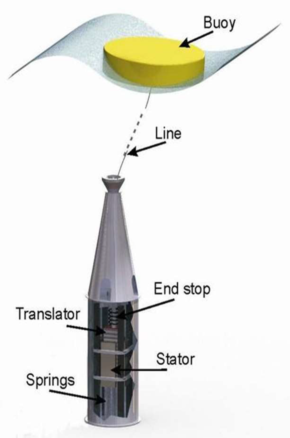
The UU-WEC (Figure 1) is a point absorber that comprises a submerged linear generator connected to a heaving buoy e.g., [33]. The WECs are connected through an offshore marine substation before the electricity is transmitted to an onshore connection point [34]. The voltage output of UU-WECs is about 450 V, and the estimated operational capacity is between of 10 kW and 100 kW but can be scaled up. The power rating can be adjusted to match the local wave climate [33,35,36], and is mostly determined by the electrical configurations and by the size and shape of the buoy and generator. These three parameters can be adjusted to fit a local wave climate. This WEC technology is currently used for offshore experiments in Lysekil on the west coast of Sweden, and the experimental research has progressed for more than ten years [33], including studies on environmental aspects of wave energy conversion. These studies revealed very limited negative impacts of the UU-WECs to the marine environment e.g., [37,38]. Instead, positive effects, such as artificial reefs, were observed [37,38]. Other recent studies on the same WEC concept include control strategies, compensations for tides and discussions on the design of wave power farms with several WECs [39,40,41].
2. Studied Region
The studied region covers the coastal area of Kilifi, located north of Mombasa in Kenya (Figure 2). The local bathymetry varies from 0 m to 30 m depth at close proximity to the beach. The seabed in this area is dominated by sedimentary rocks, loose clay, sand, mud flats, and coral reef that is normally distributed between 16 m and 45 m depth at distances from shore between 500 m to 2 km [42].
The marine environment is generally characterized by seagrass communities, mangrove forest and sandy subtracts [43]. The marine fauna is diverse and, includes sensitive species such as turtles and dugongs [42]. The wind pattern in this region is mostly dominated by monsoons, sea breeze, and occasionally cyclones. The tide in Kilifi is semi-diurnal with an amplitude of 3.5 m [27]. These tides contribute to intertidal platforms, mud flats and rather rocky communities that get exposed for several hours during low tides, and sub tidal platforms that are highly productive and populated by coral reefs, reef flats and susceptible to nearshore wave action.
3. Wave Data
The wave data used was provided by Fugro (document No. 162030-1-R0) (see Supplementary Materials). The data covers a period from January 1997 to December 2015 with a temporal resolution of 6 h, and was based on analysis of the world waves data source of the European Centre for Medium-range Weather Forecasts (ECWMF) wave model. Re-analyses were conducted by Fugro Oceanor combined with a global buoy at location with 34 m bottom depth, and multi-satellite altimeter database (Topex, Jason, Geosat, GFO and Envisat) by transforming offshore grid points to a nearshore point (3.815° S, 39.846° E) using Simulating Wave Nearshore (SWAN) model.
The data set contains wave field variables: significant wave height (Hs), mean wave energy period (Te), and mean wave direction (MDir). The variables were estimated from a wave energy spectrum (𝑓, 𝜃) with moment m0. The Hs is equivalent to the mean height of the highest one-third of the waves in a sea-state (). The Te is equivalent to the spectral period and is given by . MDir is the direction of the most energetic spectral band.
The wave power resource (Pw) was estimated using Equation (1), which defines Pw as the average transport rate of energy per meter of wave front, it depends mostly on the wave height and wave period. By definition, Pw can be affected by wave dissipation, shoaling, reflection, refraction, trapping, diffraction, and other non-linear phenomena [44,45,46].
where 𝜌 is the water density (1025 kg/m3 for sea water), 𝑔 is the acceleration due to gravity (9.8 m/s2), 𝐶𝑔 is the group velocity which depends of the water depth ℎ, 𝑓 is the frequency, and 𝜃 is the direction of propagation.
Assuming that the water depth is deep enough so that ℎ/𝐿 > 0.5, then Cg = g/4πf; therefore the simplified form of Equation (1) (in (kW/m)) becomes:
The Wave Powered Desalination Approach—An Estimation
The validation of the possibility of utilizing wave energy for desalination through RO was conducted taking into account the following parameters: Available wave power resource (), installed capacity per unit WEC (), energy per unit WEC per day at capacity factor of 30% (), energy needed per unit volume of treated water ( = 3 kWh/m3), taken from an interval between 2 kWh/m3 and 5 kWh/m3 [18,19,20,21,22]. Taking into account that the basic daily need of volume of water for one person (), is around 0.02 m3 [1]; however, this study uses m3. A fundamental question can be: How many WECs (Equation (3)) are needed to meet the water demand of the local inhabitants at daily basis?
where is the number of WECs, is the number of inhabitants, and , is the number of inhabitants supplied by freshwater from a single WEC, recalling that a 1000 L is equivalent to 1 m3.
4. Results
4.1. Local Wave Climate
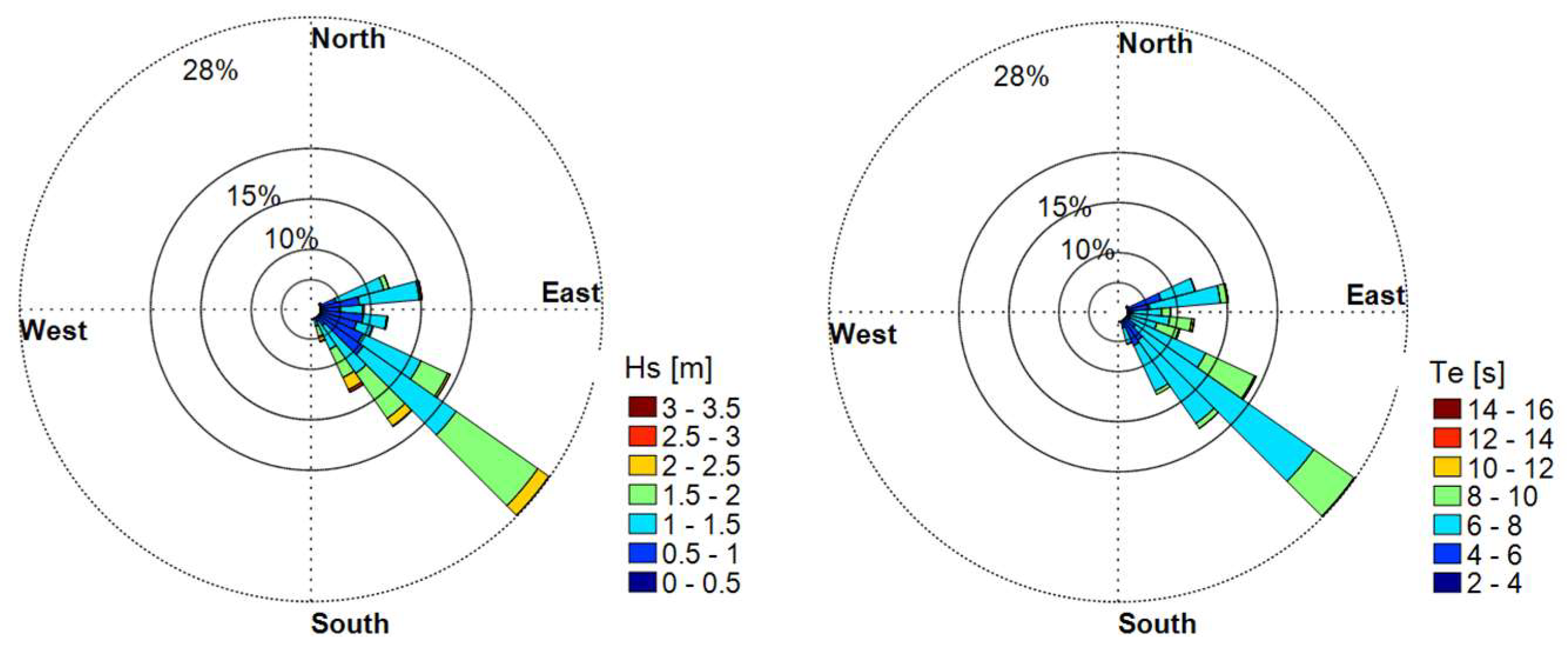
The mean value of wave power, Pw, for this data set is 7 kW/m, the median values is 5 kW/m, the mode is 5 kW/m, and the minimum and maximum are 0.2 and 53 kW/m respectively. This data reveals a wide difference of wave power between the periods of slack versus periods of high seas. It is important is to analyse the frequency of occurrence and magnitude of sea states (Figure 3, Figure 4 and Figure 5) in order to understand how the energy is distributed over time. The significant wave height, Hs, (Figure 3 and Figure 4) shows that the predominant values are within 0.75 m to 2 m, in which the southeast sea state, with a frequency of occurrence of 56%, has values of Hs in the interval between 1 m and 1.5 m. The second most dominant sea state, with 28% of occurrence, has easterly waves within 1.5–2 m. 12% of the waves compose the east-north-easterly seas state with Hs within 0.4–0.7 m. Higher sea states account for approximately 4% of occurrence and have values of Hs within 2–3 m. In what regards the wave mean period, results in Figure 3 show that the most prevalent sea state, 79% of occurrence, has values of within 7–8 s, followed by 10% of sea states with Te of 5 s, 10% with 9–10 s, and 1% for sea states with values of Te of 4 s and above 11 s, respectively.
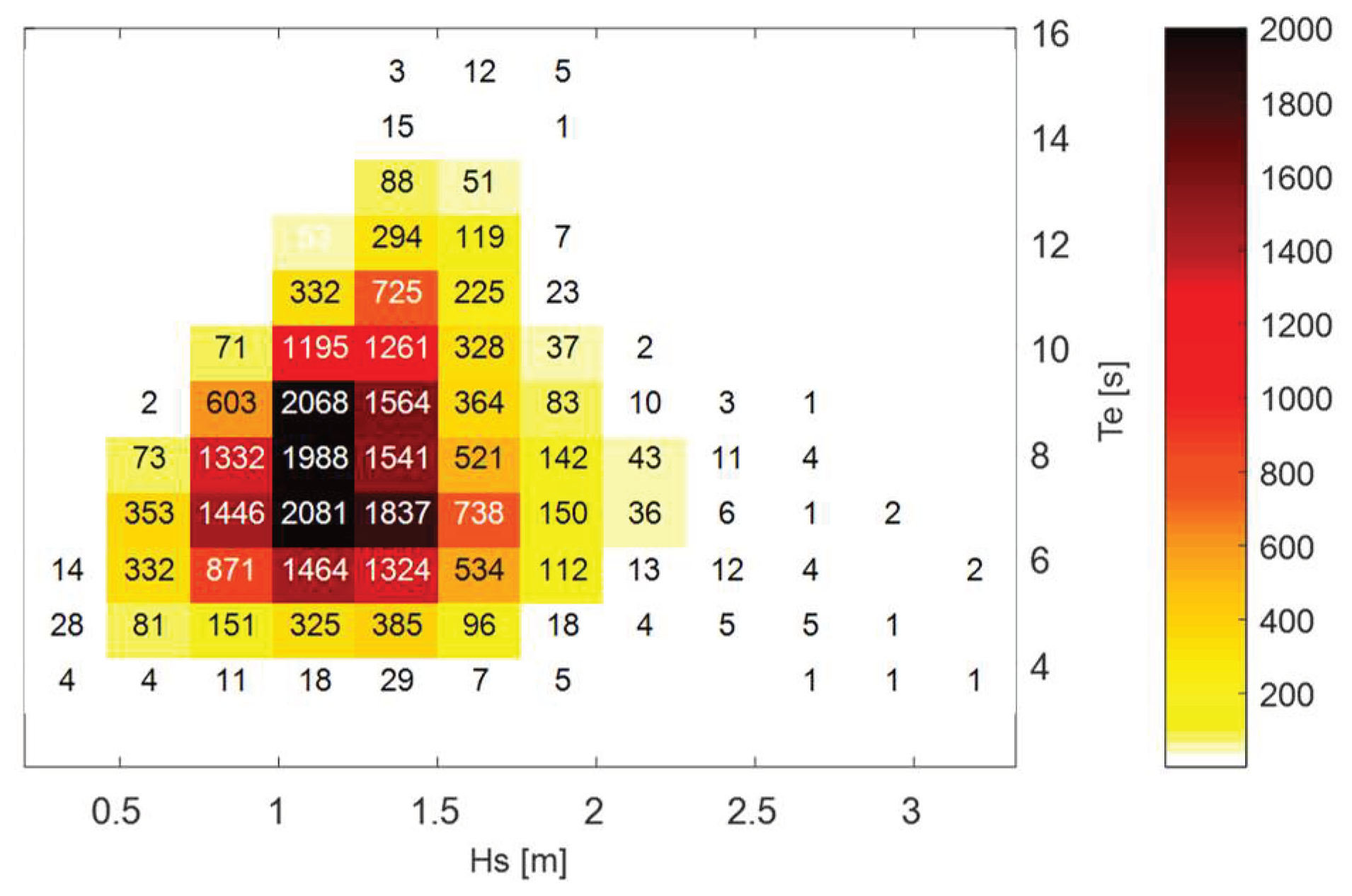
The distribution of Hs and Te (Figure 3 and Figure 4) in time also show sea states with different wave power values starting from 2 kW/m up to 50 kW/m with a higher density between 10 kW/m and 20 kW/m (Figure 5). Approximately 52% of the waves have power values within 2 kW/m–5 kW/m, 33% have Pw within 7–10 kW/m, and the remaining 15% has values of Pw greater than 12 kW/m (Figure 6).
4.2. Diurnal Variability
The results show diurnal variations on the wave power resource in Kilifi. In Figure 7, there are the mean, mode and median graphs referent to observations at midnight, six, twelve and eighteen hours. From this date it was estimated that wave power values in evening and night are in average higher than in the day. However, the highest value of mode is observed in the morning. The difference between midday and mid night mean values is about 0.3 kW/m.
4.3. Seasonal Variability
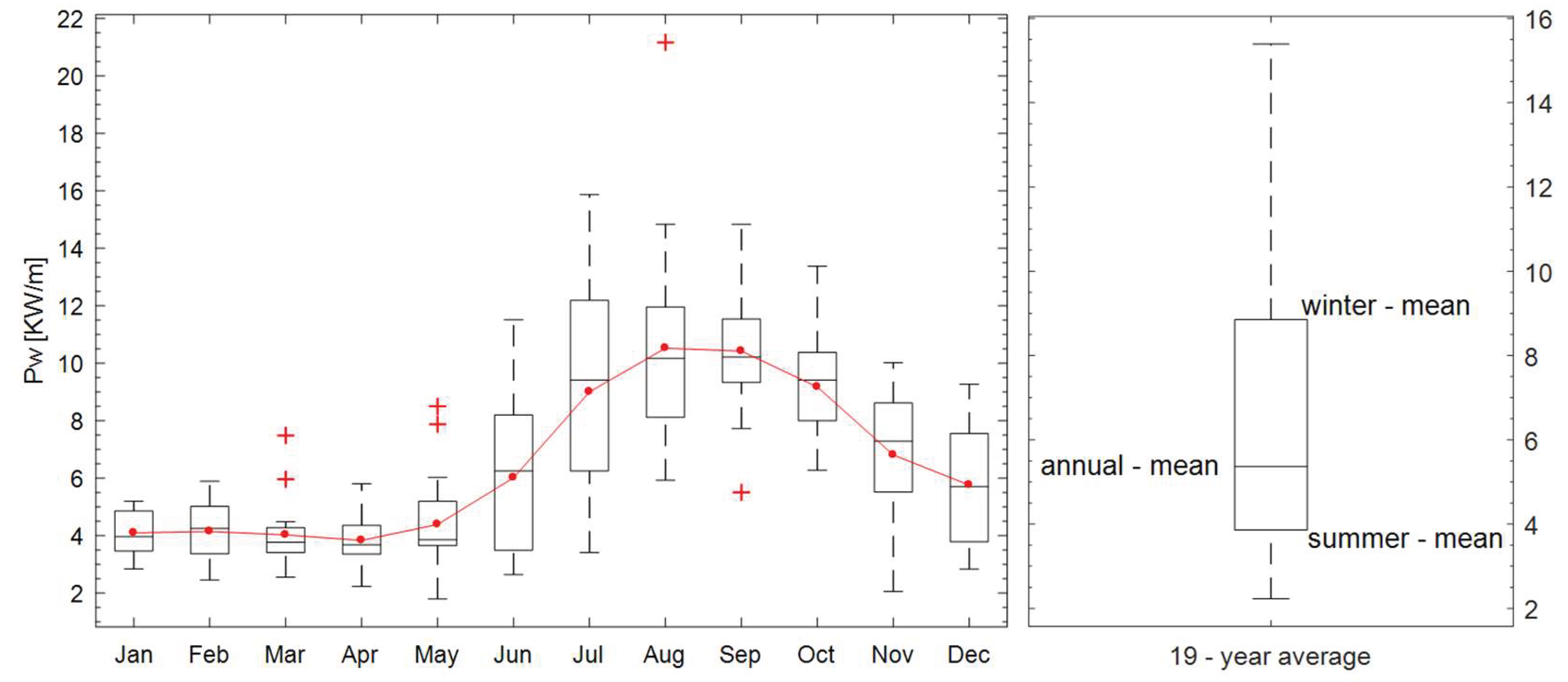
The seasonal cycle was obtained by extracting the total average for each month, over the entire time series (Figure 8: red line). There is a unimodal distribution of Pw over a period of 12 months, from January to December. Peak values are observed in August, when the mean is 10.5 kW/m followed by September with 10.2 kW/m. The box plot results shows that August and September had similar median values of approximately 10 kW/m. Although August has the highest mean, July has the highest occurrence of extreme values.
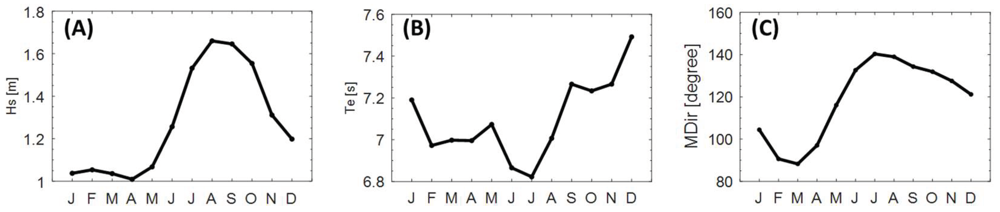
January–May had the lowest Hs mean values of approximately 1 m (Figure 9a). While July, August and September had higher mean values up to 1.5 m with a peak in August when Hs is 1.7 m. Considering Te, there are three peaks occurring in April, September and December, being the highest mean of 7.5 s. The lowest Te value, 6.8 s, was observed in July (Figure 9b). The wave mean direction MDir also had a seasonal variability signal. From February to April MDir is from east, then the waves gradually propagate from southeast from May to August, and again the mean direction reverts towards east (Figure 9c).
4.4. Interannual and Long-Term Variability
The interannual variations of Pw along the 19-year time-series are evident. The total mean is 6.5 kW/m, total standard deviation is 4.6 kW/m and the mean absolute deviation is 3.4 kW/m. For this period of time, the anomaly of Pw was calculated from the difference between the total mean and the mean of each month. Results show that there is an oscillatory pattern in the anomaly of Pw with periods of 3–5 years (Figure 10). Probably, with a longer data set, it would be possible to better detect the variability.
4.5. Wave Powered Desalination
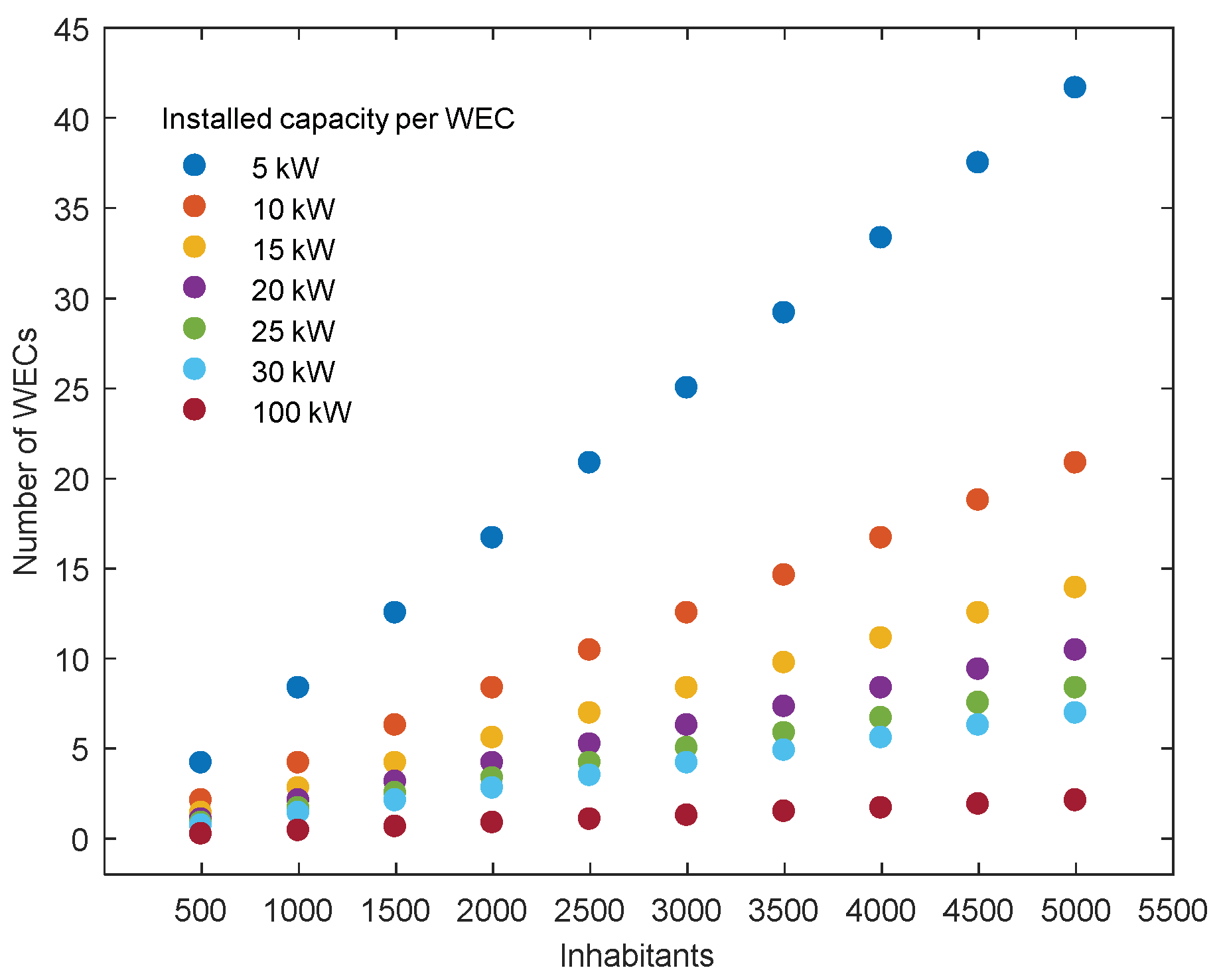
Results showed that not many WECs are needed to supply water for small communities, assuming a capacity factor of 30% (Figure 11). For example, only 10 UU-WECs with installed capacity of 20 kW per unit would be required for daily production of freshwater for about 5000 inhabitants.
5. Discussion
5.1. Wave Climate
There is a relatively high frequency of occurrence of waves with simultaneously small Hs and longer Te and vice-versa, see Figure 5. This may explain the reason why Pw occurs densely within 5 kW/m to 25 kW/m. It is also observed that the typical sea sates are determined by values of Te rather than Hs (Figure 4, Figure 5 and Figure 6). For instance, the frequency of occurrence of waves of Hs of 1–1.25 m are noticeable the highest and corresponds to values of Te that widely range from 3–9 s.
Diurnal variability of wave power may be related to the coastal wind dynamics, such as offshore and sea breezes triggered by pressure gradients due to uneven heating and cooling of the land and sea masses. In this study, the wave power’s time-variation signal share similarities in shape with the wind field’s time-variations obtained by, for example Mahongo et al. [47]. Studies on coastal wind patterns such as [47], revealed the existence of similar diurnal variations on wind intensity using three-hourly wind data of four locations along the coast of Tanzania. The wind is strongest in the afternoon (14:00–15:00), and weakest in early morning (4:00). From the wind pattern described by [47], it is possible to infer that wave power values in the second quarter of the day occur when the wind direction is from north-northeast in the austral summer and from southwest during austral winter. Peak diurnal values of wave power do occur when the wind direction are dominantly form east-northeast (austral winter) and south-southeast (austral winter).
With regard to the seasonal variability, April has the lowest mean Pw of 3.8 kW/m. The minimum monthly mean coincides with calm north-easterly wind conditions in Tanzania and Kenya, which occur in March–April and November [48,49,50]. Moreover, low values of Pw observed during the same period of the northeast monsoon (November to March). The monthly mean values of Pw differ from what was found by other authors, e.g., Barstow 2008 [51], who estimated 5–10 kW/m for January and 20–30 kW/m for July. The reason for this discrepancy may be due to the fact that they used altimetry-model data from deep water points, while the present study used data from a shallower water point. The Pw and Hs have similar seasonal variability signals (Figure 11). The maximum Hs is in contra-phase with the maximum Te may justify the reason to why there are considerably low values of Pw in this region. Other contributing factors can be latitude and weather systems including the inter-tropical convergence zone that oscillates within 15° S and 15° N and the monsoon regime [51,52]. The presence of a large land mass-Madagascar may also block larger and longer southerly waves from reaching the Kenya.
Interannual and long term variability of the wave power resources in Kilifi is influenced by local, regional and mesoscale weather systems. For example, previous studies have shown that the coastal wind in Kenya is associated with the monsoon wind system [53]. By looking at the coastal wind intensity, it is found that the shape of its seasonal cycle signal is similar to the one observed in the wave power’s signal, with peaks in July and dips in March–April. The peaks are influenced by the austral seasonality of wind and wave fields generated in the southern ocean. With the absence of such influence, the minima of wave power should be registered around December–January. However, for this particular region of the Indian Ocean, the climate dynamics are strongly influenced by the Indian Ocean Dipole, that is an oscillatory mode that couples the variability of both atmosphere and the ocean. The lowest negative mode of the Indian Ocean Dipole occurs in March–April, that coincides with the minima in the magnitude of both wind and wave power.
Calculated anomalies of Pw correlate well with monthly mean sea level pressure at the surface linked to the Southern Ocean Mode (with correlation coefficient r < −0.6), Indian Ocean Dipole (r > 0.4) and slight influenced by the El Niño (r ~ 0.4). The 3 years–4 years variability can be observed with El Niño Southern Oscillation (r ~ −0.5). There is a strong correlation between Pw and sea surface temperature of tropical and southern ocean basins (Figure 9). Studies done by Reguero et al., 2015 [54] also found significant correlation of monthly mean wave power with the North Atlantic Oscillation (r ~ 0.2), El Niño Southern Oscillation (r ~ 0.2), Atlantic Multidecadal Oscillation (r ~ −0.2) and Dipole Mode Index (r ~ −0.3).
5.2. Wave Powered Desalination
The estimative results in Figure 10 were achieved assuming that wave power has an annual capacity factor near 30%. Several studies suggest that the capacity factor of wave power is ca. 20–40% at the most [55,56,57,58]. Being so, the number of WECs (20 kW) required for a daily supply of freshwater to 5000 inhabitants would increase or decrease in function of the capacity factor. Moreover, the capacity factor would vary seasonally, being lower during austral summer months (January to May) and higher during July to November. On the other hand, the number of required WECs would also vary according to the efficiency of the desalination system in terms of energy consumption. For example, similarly to above, assuming a capacity factor of 30%, but with an energy consumption of 2 kWh/m3, the required number of WECs (20 kW) for 5000 inhabitants would decrease to seven units.
The results indicate a mild wave climate in Kilifi. This is particularly suitable for the UU-WEC technology that is versatile to variety of wave steepness. Due to few extreme wave days and lower forces acting on the system—reducing the risk of technical failure, and lowering its predicted maintenance. The UU-WEC was designed to optimally operate in depths within 20 m and 50 m, in rather flat seabed, conditions which normally occur in Kilifi and on other coastal areas across the globe. Several layout designs of wave power farms can be used to maximize energy abortion, as described in [59,60,61]. In practice, these wave power farm layouts should also consider the distance between devices, substation and onshore cable connections which are key elements for cost reduction and feasibility, as described in [62,63]. In the case of Kilifi where a rather small number of WECs is required, a rather simple and cost effective wave power farm would be required. For example, it would include an array of WECs deployed along the same isobaths in order to maximize energy absorption.
Compared to the other wave climates, such as of the North Atlantic [54], the waves in Kenya are more predictable, which may enhance the reliability and predictability of the power or freshwater production from a wave powered desalination plant. Therefore, the use of UU-WEC for desalination purposes would be suitable to similar coastal areas where the water need is severe, requiring a reliable source of drinking water, irrigation among other purposes. Apart from the resource assessments aspects, the costs of electricity, water production and the entire life cycle of a project should be holistically analyzed.
6. Conclusions
The wave climate in Kilifi is mild, with mean values of 1.3 m, 7.1 s, and 6.5 kW/m for Hs, Te, and Pw, respectively. The difference in monthly mean values between the lower and higher seasons was in the order of ±0.7 m for Hs and of about ± 6.5 kW/m for Pw. This is due to the entire region is located within the tropical and equatorial zone where the weather patterns experience only gradual changes and the variations are rather small. The dynamics of the sea breezes and coastal winds influence the local wave power resource which is higher in the evening and night comparing to daytime values, with an estimated difference of 0.3 kW/m. The seasonal signal indicated that Pw and Hs share the same pattern in which both have peaks in August, while the dip occurred between January and May. In contrast, Te have maxima in February, May and September, whereas the minima are in February, July and October. This seasonal variability of wave power is also similar in pattern with the coastal winds, and both are conditioned by the seasonality of the monsoon system and the inter-tropical convergence zone. The interannual variability has anomalies within 2 kW/m with periodicity of 3 years to 5 years, which can be influenced by mesoscale weather and climate systems such as Indian Ocean Dipole, Southern Ocean Mode, El Niño Southern Oscillation.
The wave power resource available at the Kenyan coast is estimated to be enough for wave power conversion throughout an entire annual cycle. The peak of wave power availability and conversion would be in the austral winter that match the dry season when freshwater is needed the most. This fact highlights the importance of a desalination plant powered by WECs in arid and remote coastal areas. Assuming a capacity factor of 30% and energy consumption of 3 kWh/m3, a rather small coastal community of about five thousand inhabitants can be provided of freshwater by only ten WECs with installed capacity of 20 kW a unit, and certainly the number of WECs would decrease with the decrease of energy consumption and/or with an increase of installed capacity. There are still grey areas in what regards techno-economic and life cycle analysis of such projects involving renewable energy technologies. Uncertainties are even higher with non-stablished technologies such as wave power. Notwithstanding, near future projections appoints to reduction of energy consumption to below 3 kWh/m3 [23], and a possible decrease of water production costs [64]. On the other hand, there will be an increasing freshwater consumption which reflects on growing investments on desalination plants around the world. It is only left to the renewable energy sector to promote itself to competitive standards within the energy-water nexus. This brings us to a final conclusion that the electricity needed to run a desalination plant or any other type of electric water treatment system, can be technically supplied by renewable energy sources such as wave power.
7. Future Work
The present work is part of a larger study being undertaken by Uppsala University on use of wave power for freshwater production through desalination, with focus on the UU-WEC technology. Therefore, after investigating the wave climate in Kilifi and introducing the idea of utilizing WECs as potential power supplier, the following steps would proceed: Full description of the power system with several UU-WECs including voltage amplitude and frequency variations; Then, coupling of the power system with a RO desalination plant in Kenya that will include an energy storage system and freshwater storage seen as buffer for shifting power rates; Techno-economic and life cycle analysis would be investigated; assessment of local environmental parameters such as seabed conditions, residue management among other aspects required by law would precede a possible deployment of WECs that would culminate with an implementation of wave powered desalination system. The aforementioned steps may not follow the presented sequential order. Even so, research is needed before producing freshwater using the UU-WEC or similar technologies. The success of projects such as this, would revolutionize rural electrification in remote and coastal areas across the globe.
Supplementary Materials
The following are available online at https://www.mdpi.com/1996-1073/11/4/1004/s1, the wave data used was provided by Fugro (document No. 162030-1-R0) and can be accessed upon a request to the authors.
Acknowledgments
This project has received funding from the European Union’s Seventh Framework Programme for research, technological and demonstration under grant agreement No. 607656. This work was conducted within the STandUP for Energy strategic research framework and was also supported by the Swedish Research Council (VR) grant No. 2015-03126.
Author Contributions
Francisco Francisco wrote the paper, contributed with conception of the work, data analysis and interpretation; Jennifer Leijon contributed with conception of the work, data interpretation, drafting and revision of the manuscript; Cecilia Boström contributed with data acquisition conception of the work and revision of the manuscript; Jens Engström contributed with data acquisition, conception of the work and revision of the manuscript; Jan Sundberg contributed with conception of the work, and revision of the manuscript.
Conflicts of Interest
The authors declare no conflict of interest.
References
- UN-Water. Water for a Sustainable World; The United Nations World Water Development Report 2015; UN-Water: Geneva, Switzerland, 2015. [Google Scholar]
- Kaniaru, W. From scarcity to security: Water as a potential factor for conflict and cooperation in Southern Africa. S. Afr. J. Int. Aff. 2015, 22, 381–396. [Google Scholar] [CrossRef]
- Almer, C.; Laurent-lucchetti, J.; Oechslin, M. Water scarcity and rioting: Disaggregated evidence from Sub-Saharan Africa. J. Environ. Econ. Manag. 2017, 86, 193–209. [Google Scholar] [CrossRef]
- United Nations Educational, Scientific and Cultural Organization. Water and Jobs; The United Nations World Water Development Report 2016; United Nations Educational, Scientific and Cultural Organization: Paris, France, 2016. [Google Scholar]
- World Health Organization (WHO) and the United Nations Children’s Fund (UNICEF). Progress on Drinking Water, Sanitation and Hygiene. 2017. Available online: http://www.who.int/mediacentre/news/releases/2017/launch-version-report-jmp-water-sanitation-hygiene.pdf (accessed on 20 August 2017).
- WHO/Unicef (JMP). WASH in the 2030 Agenda; World Health Organization: Geneva, Switzerland, 2016. [Google Scholar]
- Gulati, M.; Jacobs, I.; Jooste, A.; Naidoo, D.; Fakir, S. The water-energy-food security nexus: Challenges and opportunities for food security in South Africa. Aquat. Procedia 2013, 1, 150–164. [Google Scholar] [CrossRef]
- Shikuku, K.M.; Winowiecki, L.; Twyman, J.; Eitzinger, A.; Perez, J.G.; Mwongera, C.; Läderach, P. Smallholder farmers’ attitudes and determinants of adaptation to climate risks in East Africa. Clim. Risk Manag. 2017, 16, 234–245. [Google Scholar] [CrossRef]
- Ochieng, J.; Kirimi, L.; Mathenge, M. Effects of climate variability and change on agricultural production: The case of small scale farmers in Kenya. NJAS-Wagen. J. Life Sci. 2016, 77, 71–78. [Google Scholar] [CrossRef]
- Ouma, C. Tewa Training Centre Report: Field Report for Tewa Training Centre as a Case Study under “Water Desalination Using Wave Power” Uppsala University Research Coordinated through Strathmore Energy Research Centre; Internal report at Uppsala University: Uppsala, Sweden, 2013. [Google Scholar]
- González, D.; Amigo, J.; Suárez, F. Membrane distillation: Perspectives for sustainable and improved desalination. Renew. Sustain. Energy Rev. 2017, 80, 238–259. [Google Scholar] [CrossRef]
- El-Dessouky, H.T.; Ettouney, H.M. Fundamentals of Salt Water Desalination; Elsevier: New York, NY, USA, 2002. [Google Scholar] [CrossRef]
- Shenvi, S.S.; Isloor, A.M.; Ismail, A.F. A review on RO membrane technology: Developments and challenges. Desalination 2015, 368, 10–26. [Google Scholar] [CrossRef]
- Scarazzato, T.; Panossian, Z.; Tenório, J.A.S.; Pérez-Herranz, V.; Espinosa, D.C.R. A review of cleaner production in electroplating industries using electrodialysis. J. Clean. Prod. 2017, 168, 1590–1602. [Google Scholar] [CrossRef]
- Nayar, K.G.; Sundararaman, P.; Schacherl, J.D.; O’Connor, C.L.; Heath, M.L.; Orozco Gabriel, M.; Wright, N.C.; Winter, A.G. Feasibility study of an electrodialysis system for in-home water desalination in urban India. Dev. Eng. 2016, 2, 38–46. [Google Scholar] [CrossRef]
- Khoshrou, I.; Nasr, M.R.J.; Bakhtari, K. New opportunities in mass and energy consumption of the Multi-Stage Flash Distillation type of brackish water desalination process. Sol. Energy 2017, 153, 115–125. [Google Scholar] [CrossRef]
- Van der Bruggen, B.; Vandecasteele, C. Distillation vs. membrane filtration: Overview of process evolutions in seawater desalination. Desalination 2002, 143, 207–218. [Google Scholar] [CrossRef]
- Khayet, M. Solar desalination by membrane distillation: Dispersion in energy consumption analysis and water production costs (a review). Desalination 2013, 308, 89–101. [Google Scholar] [CrossRef]
- Will, M.; Klinko, K. Optimization of seawater RO systems design. 2001, 138, 299–306. [Google Scholar]
- Banat, F.; Jwaied, N.; Rommel, M.; Koschikowski, J. Performance evaluation of the ‘large SMADES’ autonomous desalination solar-driven membrane distillation plant in Aqaba, Jordan. Desalination 2007, 217, 17–28. [Google Scholar] [CrossRef]
- Miller, J.E. Review of Water Resources and Desalination Technologies; U.S. Department of Commerce: Washington, DC, USA, 2003.
- Glueckstern, P. The impact of R & D on new technologies, novel design concepts and advanced operating procedures on the cost of water desalination. Desalination 2001, 139, 217–228. [Google Scholar]
- Energy, D.; Elimelech, M.; Phillip, W.A. The Future of Seawater and the Environment. Science 2011, 333, 712–718. [Google Scholar]
- Tzen, E.; Morris, R. Renewable energy sources for desalination. Sol. Energy 2003, 75, 375–379. [Google Scholar] [CrossRef]
- Charlier, R.H.; Justus, J.R. Ocean. Energies: Environmental, Economic and Technological Aspects of Alternative Power Sources; Elsevier Science: New York, NY, USA, 1993. [Google Scholar]
- Doukas, H.; Karakosta, C.; Psarras, J. {RES} technology transfer within the new climate regime: A ‘helicopter’ view under the {CDM}. Renew. Sustain. Energy Rev. 2009, 13, 1138–1143. [Google Scholar] [CrossRef]
- Hammar, L. Towards Technology Assessment of Ocean. Energy in a Developing Country Context. Licentiate Thesis, Chalmers University of Technology, Gothenburg, Sweden, 2011. [Google Scholar]
- de O. Falcão, A.F. Wave energy utilization: A review of the technologies. Renew. Sustain. Energy Rev. 2010, 14, 899–918. [Google Scholar]
- Davies, P.A. Wave-powered desalination: Resource assessment and review of technology. Desalination 2005, 186, 97–109. [Google Scholar] [CrossRef]
- Khan, N.; Kalair, A.; Abas, N.; Haider, A. Review of ocean tidal, wave and thermal energy technologies. Renew. Sustain. Energy Rev. 2017, 72, 590–604. [Google Scholar] [CrossRef]
- Cornett, A.M. A Global Wave Energy Resource Assessment. In Proceedings of the International Offshore and Polar Engineering Conference, Busan, Korea, 15–20 June 2014. [Google Scholar]
- Gunn, K.; Stock-Williams, C. Quantifying the global wave power resource. Renew. Energy 2012, 44, 296–304. [Google Scholar] [CrossRef]
- Lejerskog, E.; Boström, C.; Hai, L.; Waters, R.; Leijon, M. Experimental results on power absorption from a wave energy converter at the Lysekil wave energy research site. Renew. Energy 2015, 77, 9–14. [Google Scholar] [CrossRef]
- Ekström, R.; Baudoine, A.; Rahm, M.; Leijon, M. Marine substation design for grid-connection of a research wave power plant on the Swedish West coast. In Proceedings of the 10th European Wave and Tidal Conference, Aalborg, Denmark, 2–5 September 2013. [Google Scholar]
- Leijon, M.; Boström, C.; Danielsson, O.; Gustafsson, S.; Haikonen, K.; Langhamer, O.; Strömstedt, E.; Stålberg, M.; Sundberg, J.; Svensson, O.; et al. Wave energy from the North Sea: Experiences from the lysekil research site. Surv. Geophys. 2008, 29, 221–240. [Google Scholar] [CrossRef]
- Bostrom, C.; Ekergard, B.; Waters, R.; Eriksson, M.; Leijon, M. Linear generator connected to a resonance-rectifier circuit. IEEE J. Ocean. Eng. 2013, 38, 255–262. [Google Scholar] [CrossRef]
- Langhamer, O.; Haikonen, K.; Sundberg, J. Wave power-Sustainable energy or environmentally costly? A review with special emphasis on linear wave energy converters. Renew. Sustain. Energy Rev. 2010, 14, 1329–1335. [Google Scholar] [CrossRef]
- Haikonen, K. Underwater Radiated Noise from Point Absorbing Wave Energy Converters. Ph.D. Thesis, Uppsala University, Uppsala, Sweden, 2014. [Google Scholar]
- Wang, L.; Isberg, J. Nonlinear passive control of a wave energy converter subject to constraints in irregular waves. Energies 2015, 8, 6528–6542. [Google Scholar] [CrossRef]
- Ekström, R.; Ekergård, B.; Leijon, M. Electrical damping of linear generators for wave energy converters—A review. Renew. Sustain. Energy Rev. 2015, 42, 116–128. [Google Scholar] [CrossRef]
- Castellucci, V.; Abrahamsson, J.; Kamf, T.; Waters, R. Nearshore tests of the tidal compensation system for point-absorbing wave energy converters. Energies 2015, 8, 3272–3291. [Google Scholar] [CrossRef]
- Tychsen, J. (Ed.) KenSea. Environmental Sensitivity Atlas for Coastal Area of Kenya; Geological Survey of Denmark and Greenland (GEUS): Copenhagen, Denmark, 2006; 76p, ISBN 87-7871-191-6. [Google Scholar]
- Obura, D.O. Kenya. Mar. Pollut. Bull. 2001, 42, 1264–1278. [Google Scholar] [CrossRef]
- Liu, P.L.F.; Losada, I.J. Wave propagation modeling in coastal engineering. J. Hydraul. Res. 2002, 40, 229–240. [Google Scholar] [CrossRef]
- Gorrell, L.; Raubenheimer, B.; Elgar, S.; Guza, R.T. SWAN predictions of waves observed in shallow water onshore of complex bathymetry. Coast. Eng. 2011, 58, 510–516. [Google Scholar] [CrossRef]
- World Meteorological Organization. Guide to Wave Analysis Guide to Wave Analysis; World Meteorological Organization: Geneva, Switzerland, 1998. [Google Scholar]
- Mahongo, S.B.; Francis, J.; Osima, S.E. Wind Patterns of Coastal Tanzania: Their Variability and Trends. West. Indian Ocean J. Mar. Sci. 2012, 10, 107–120. [Google Scholar]
- Mcclanahan, T.R. Seasonality in East Africa’s coastal waters. Mar. Ecol. Prog. Ser. 1988, 44, 191–199. [Google Scholar] [CrossRef]
- Hammar, L.; Ehnberg, J.; Mavume, A.; Cuamba, B.C.; Molander, S. Renewable ocean energy in the Western Indian Ocean. Renew. Sustain. Energy Rev. 2012, 16, 4938–4950. [Google Scholar] [CrossRef]
- Camberlin, P. Oxford Research Encyclopedia of Climate Science Climate of Eastern Africa Geographical Features Influencing the Region ’ s Climate; Oxford University Press: Oxford, UK, 2018; No. April. [Google Scholar]
- Barstow, S.; Mørk, G.; Lønseth, L.; Mathisen, J.P. WorldWaves wave energy resource assessments from the deep ocean to the coast. In Proceedings of the 8th European Wave Tidal Energy Conference, Uppsala, Sweden, 7–10 September 2009; pp. 149–159. [Google Scholar]
- Semedo, A. Seasonal Variability of Wind Sea and Swell Waves Climate along the Canary Current : The Local Wind Effect. J. Mar. Sci. Eng. 2018, 6. [Google Scholar] [CrossRef]
- Francis, J. Wind patterns of coastal Tanzania: Their variability and trends Wind Patterns of Coastal Tanzania: Their Variability. West. Indian Ocean J. Mar. Sci. 2012, 10, 107–120. [Google Scholar]
- Reguero, B.G.; Losada, I.J.; Méndez, F.J. A global wave power resource and its seasonal, interannual and long-term variability. Appl. Energy 2015, 148, 366–380. [Google Scholar] [CrossRef]
- Ibarra-Berastegi, G.; Jon, S.; Garcia-soto, C. Electricity production, capacity factor, and plant efficiency index at the Mutriku wave farm (2014–2016). Ocean Eng. 2018, 147, 20–29. [Google Scholar] [CrossRef]
- World Energy Council. World Energy Resources Marine Energy|2016; World Energy Council: London, UK, 2016. [Google Scholar]
- David Kavanagh, B.E. Capacity Value of Wave Energy in Ireland. Master’s Thesis, University College Dublin, Dublin, Ireland, 2012. [Google Scholar]
- Stoutenburg, E.D.; Jenkins, N.; Jacobson, M.Z. Power output variations of co-located offshore wind turbines and wave energy converters in California. Renew. Energy 2010, 35, 2781–2791. [Google Scholar] [CrossRef]
- Göteman, M.; Engström, J.; Eriksson, M.; Isberg, J. Fast Modeling of Large Wave Energy Farms Using Interaction Distance Cut-Off. Energies 2015, 8, 13741–13757. [Google Scholar] [CrossRef]
- Giassi, M.; Malin, G. Parameter Optimization in Wave Energy Design by a Genetic Algorithm. In Proceedings of the 2015 International Congress on Technology, Communication and Knowledge (ICTCK), Mashhad, Iran, 11–12 November 2017; pp. 23–26. [Google Scholar]
- Giassi, M.; Malin, G.; Thomas, S.; Engstr, J.; Eriksson, M.; Isberg, J. Multi-Parameter Optimization of Hybrid Arrays of Point Absorber Wave Energy Converters. In Proceedings of the 12th European Wave and Tidal Energy Conference (EWTEC), Cork, Ireland, 27–31 August 2017; pp. 1–6. [Google Scholar]
- Chatzigiannakou, M.A.; Dolguntseva, I.; Leijon, M. Offshore Deployments of Wave Energy Converters by Seabased Industry AB. J. Mar. Sci. Eng. 2017, 5, 15. [Google Scholar] [CrossRef]
- Dolguntseva, I. Offshore deployment of marine substation in the Lysekil research site. In Proceedings of the The 25th International Ocean and Polar Engineering Conference, Kona, HA, USA, 21–26 June 2015. [Google Scholar]
- Voutchkov, N. Desalination—Past, Present and Future. International Water Association, 2016. Available online: http://www.iwa-network.org/desalination-past-present-future/ (accessed on 16 March 2018).
Figure 1.
Comprehensive illustration of Uppsala University’s main WEC concept, comprising of a linear generator on the ocean floor, with a movable part (the translator) connected via a line to a buoy.
Figure 1.
Comprehensive illustration of Uppsala University’s main WEC concept, comprising of a linear generator on the ocean floor, with a movable part (the translator) connected via a line to a buoy.

Figure 2.
Studied location in Kilifi (3.815° S, 39.846° E), ca. 60 km north of Mombasa, Kenya. The Yellow dashed circle represents the data extraction point (Fugro-No. 162230-1-R0). Local bathymetry and costal features are shown within the circle.
Figure 2.
Studied location in Kilifi (3.815° S, 39.846° E), ca. 60 km north of Mombasa, Kenya. The Yellow dashed circle represents the data extraction point (Fugro-No. 162230-1-R0). Local bathymetry and costal features are shown within the circle.
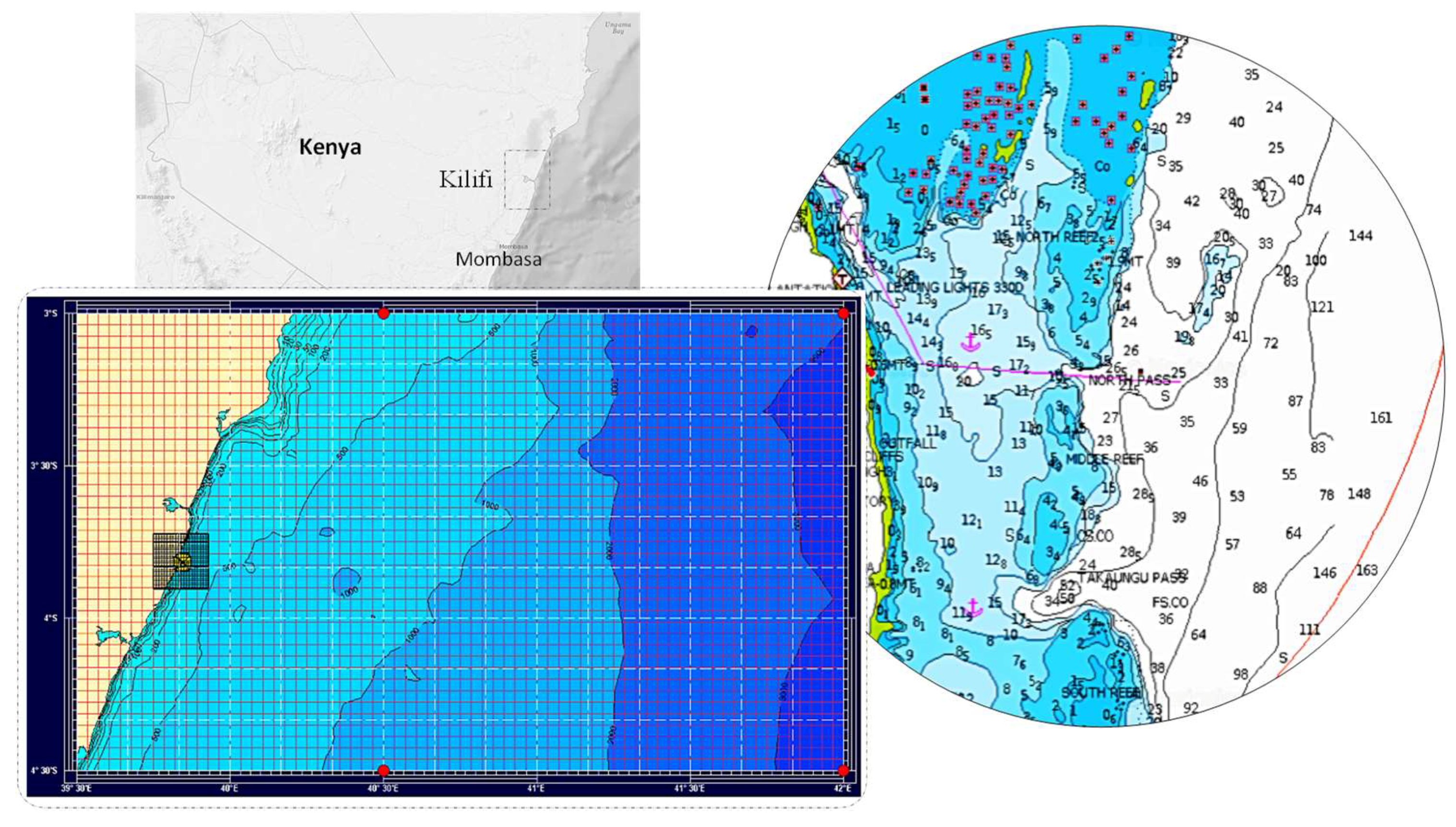
Figure 3.
Total probability distribution of significant wave height Hs wave mean period Te and wave mean direction versus mean wave direction MDir in Kilifi. The frequencies of occurrence of sea states are given in percentage.
Figure 3.
Total probability distribution of significant wave height Hs wave mean period Te and wave mean direction versus mean wave direction MDir in Kilifi. The frequencies of occurrence of sea states are given in percentage.

Figure 4.
Total probability distribution of sea sates at six-hourly occurrence in Kilifi.

Figure 5.
Combined scatter plot showing the occurrence of Hs, Te and Pw in Kilifi.
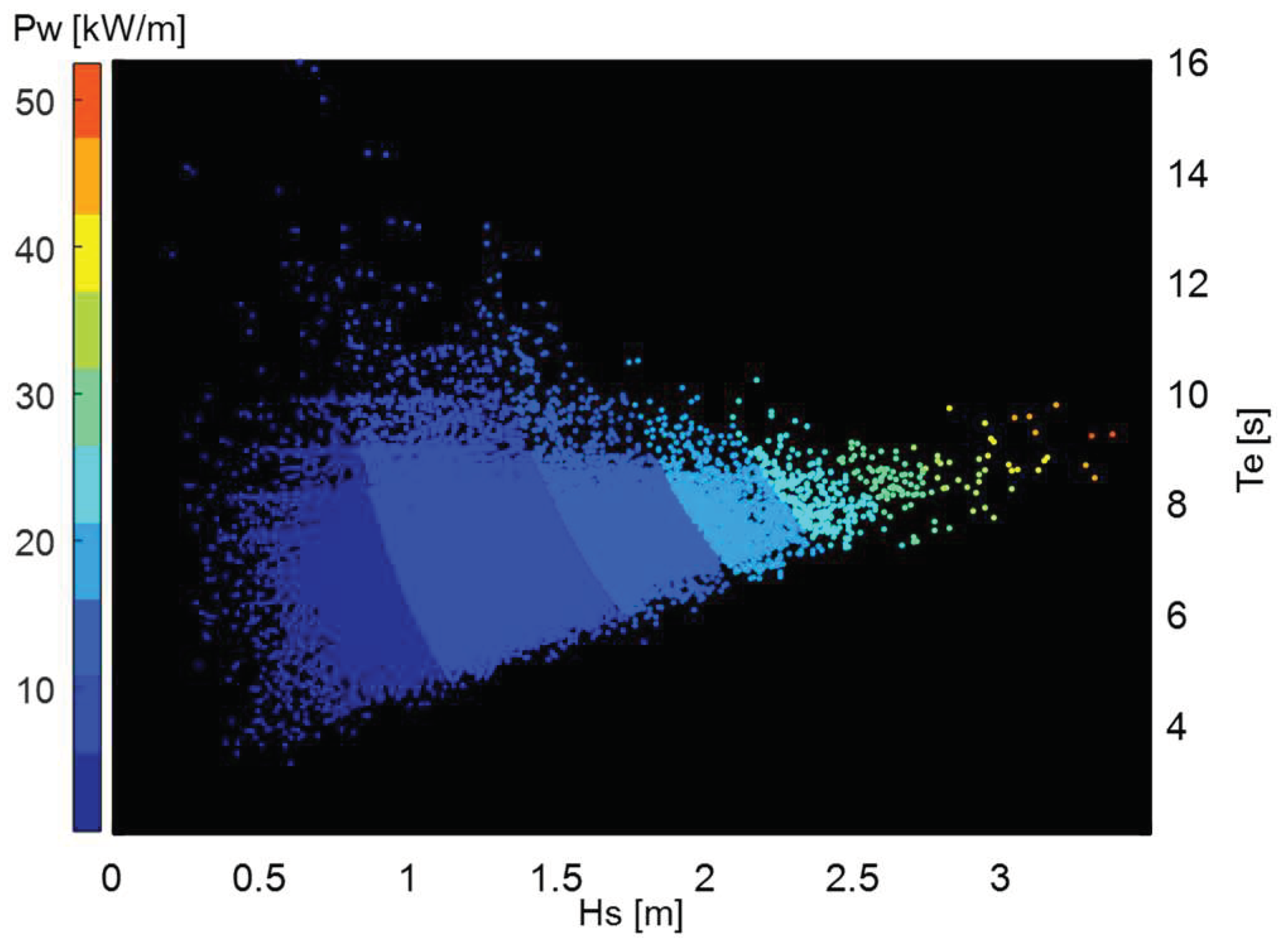
Figure 6.
Total probability distribution of wave power Pw versus mean wave direction MDir. The frequencies of occurrence of sea states are given in percentage in Kilifi.
Figure 6.
Total probability distribution of wave power Pw versus mean wave direction MDir. The frequencies of occurrence of sea states are given in percentage in Kilifi.
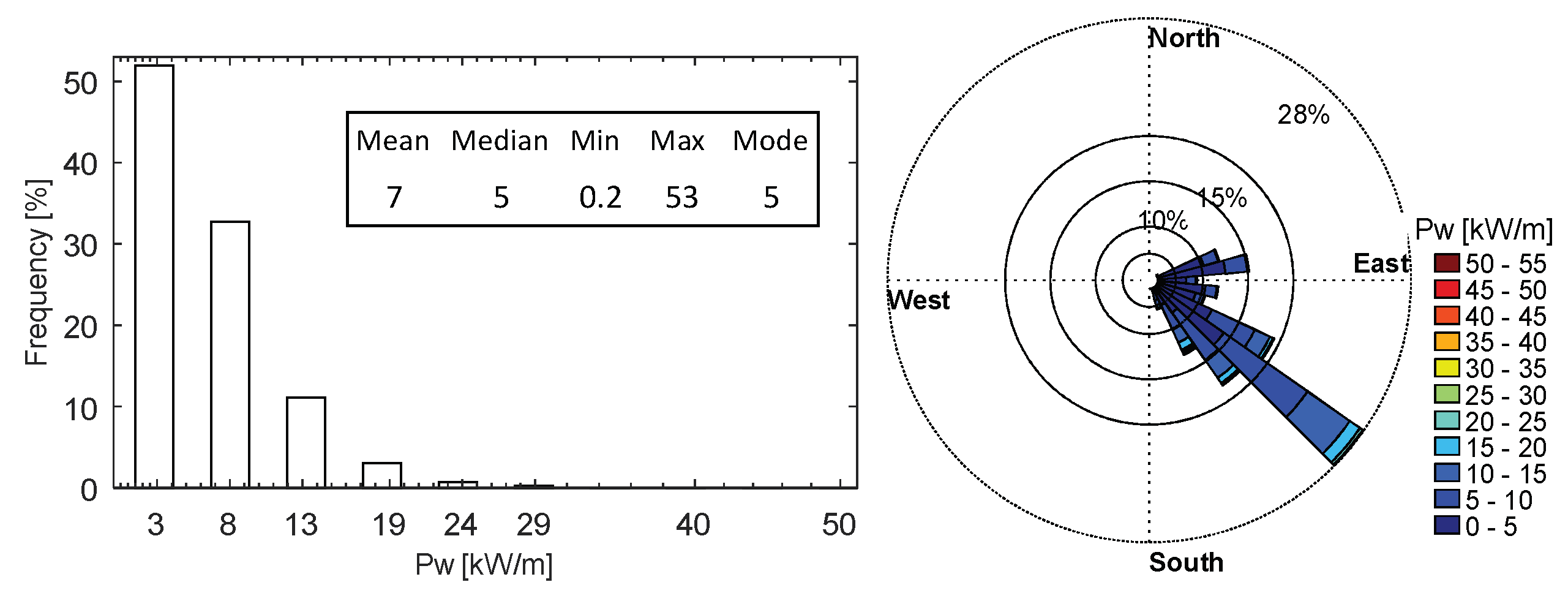
Figure 7.
Diurnal variability of wave power in Kilifi based on 6–hourly wave data, showing lower values during day comparing to night.
Figure 7.
Diurnal variability of wave power in Kilifi based on 6–hourly wave data, showing lower values during day comparing to night.
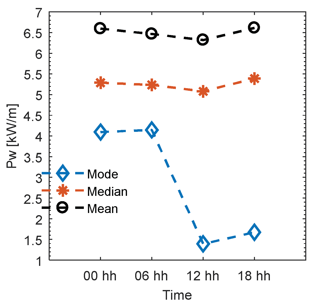
Figure 8.
The seasonal variability of Pw in Kilifi. The red line represents monthly mean values of Pw, the box plot contains the median-middle mark, the 25th and 75th percentiles—the bottom and top edges of the box, respectively. The red crosses are outliers of Pw, representing for example storms and tropical cyclones.

Figure 9.
The seasonal variability in Kilifi: (A) for Hs; (B) for Te; and (C) for MDir. Te (B) has a rather different pattern with three-modal seasonal variability compared with a unimodal pattern observed in both Hs (A) and MDir (C) respectively.
Figure 9.
The seasonal variability in Kilifi: (A) for Hs; (B) for Te; and (C) for MDir. Te (B) has a rather different pattern with three-modal seasonal variability compared with a unimodal pattern observed in both Hs (A) and MDir (C) respectively.

Figure 10.
Pw from 1997 to 2016 in Kilifi, plotted as annual mean (black dots) and respective anomalies (red bars).
Figure 10.
Pw from 1997 to 2016 in Kilifi, plotted as annual mean (black dots) and respective anomalies (red bars).

Figure 11.
Number of WECs necessary for daily freshwater production as a function of number of inhabitants and installed capacity per unit WEC assuming a capacity factor of 30% and fixed energy consumption of 3 kWh/m3.
Figure 11.
Number of WECs necessary for daily freshwater production as a function of number of inhabitants and installed capacity per unit WEC assuming a capacity factor of 30% and fixed energy consumption of 3 kWh/m3.
© 2018 by the authors. Licensee MDPI, Basel, Switzerland. This article is an open access article distributed under the terms and conditions of the Creative Commons Attribution (CC BY) license (http://creativecommons.org/licenses/by/4.0/).
Share and Cite
MDPI and ACS Style
Francisco, F.; Leijon, J.; Boström, C.; Engström, J.; Sundberg, J. Wave Power as Solution for Off-Grid Water Desalination Systems: Resource Characterization for Kilifi-Kenya. Energies 2018, 11, 1004. https://doi.org/10.3390/en11041004
AMA Style
Francisco F, Leijon J, Boström C, Engström J, Sundberg J. Wave Power as Solution for Off-Grid Water Desalination Systems: Resource Characterization for Kilifi-Kenya. Energies. 2018; 11(4):1004. https://doi.org/10.3390/en11041004
Chicago/Turabian StyleFrancisco, Francisco, Jennifer Leijon, Cecilia Boström, Jens Engström, and Jan Sundberg. 2018. "Wave Power as Solution for Off-Grid Water Desalination Systems: Resource Characterization for Kilifi-Kenya" Energies 11, no. 4: 1004. https://doi.org/10.3390/en11041004
Note that from the first issue of 2016, this journal uses article numbers instead of page numbers. See further details here.