Research on Economic Comprehensive Control Strategies of Tractor-Planter Combinations in Planting, Including Gear-Shift and Cruise Control

State Key Laboratory of Mechanical Transmissions, Chongqing University, Chongqing 400044, China
*
Author to whom correspondence should be addressed.
Energies 2018, 11(3), 686; https://doi.org/10.3390/en11030686
Submission received: 27 January 2018
/
Revised: 11 March 2018
/
Accepted: 12 March 2018
/
Published: 19 March 2018
Abstract
:An automatic control strategy for forward speed in the planting process is proposed to improve the fuel economy and reduce the labor intensity of drivers. Models of tractors with power-shift transmission (PST) and a precise pneumatic planter with an electric-driven seed metering device are built as research objects and simulated using Matlab with Simulink. The economic comprehensive control strategies for forward speed, including gear-shift schedule and cruise control strategy, are developed. Four levels control mode with different fuel economy performances are implemented to meet different driver or operation condition requirements. In addition, the control strategy is developed for the seed-metering device motor to maintain the required seed spacing in planting. Finally, the fuel economy and effectiveness of the control strategies for forward speed and planting quality are verified by simulations with Matlab/Simulink and Matlab/Stateflow. The simulation results verify the satisfactory performance of the proposed control strategies. The error of seed spacing is less than 3% when planting with speed fluctuation. Under the premise of ensuring planting quality and driver’s demands, the cruise control strategies for forward speed have more significant effects on the fuel economy than previous cruise control strategies. Furthermore, the control mode with higher level has better fuel economy and a larger speed deviation range.
1. Introduction
With the development of precision agriculture [1], the tractor is developing as major and crucial power machinery towards the use of intelligence and informatization in agriculture. Studies on intelligent tractors mainly focus on automatic navigation control, especially on the steering control and algorithms for positioning in navigation [2,3,4,5,6], and theoretical studies of automatic control of tractor speed and gear-shift schedules are lacking.
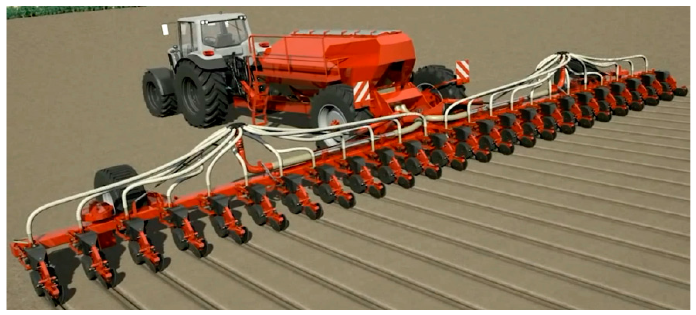
In order to reduce the labor intensity of drivers in the operating process of tractors with agricultural implements (tractor-implement combinations), cruise control is a better choice for operating conditions with light loads (such as planting, spraying, etc.) whose operating speed is relatively stable during single-pass operation [7]. The tractors with different agricultural implements has different power flows and operating characteristics, so different control strategies must be developed for gear shifting and cruise control. In this paper, a tractor with a power-shift transmission combined with a pneumatic precision planter, which is illustrated in Figure 1, is chosen as research object. The main purpose of this paper is to provide an economic comprehensive cruise control strategy, including the gear-shifting schedule, for a tractor-planter combination under planting operation conditions, which is rarely studied by other researchers.
Cruise control has been widely used in the automobile field. Research on cruise control for road vehicles has attracted much attention from many scholars [8]. Nevertheless, they mainly focused on achieving precise control of vehicle speed or maintaining a steady gap from the preceding vehicle, which is used to ensure safety and avoid violating road regulations when traveling on roads [9,10]. There are significant differences in the traveling conditions between road and farm vehicles.
In the field of agricultural machinery, some researchers have studied speed control methods for different objects [11,12,13,14]. Model-based predictive control was used to implement cruise control on a combine harvester to which a diesel engine and a variable hydraulic pump supplied the power [11,12]. A multi-parameter fuzzy control strategy was used to control the forward speed of a combine harvester based on the knowledge discovery in databases [13]. A variable universe adaptive fuzzy-PID (proportional–integral–derivative) control method was used to improve the adaptability of control algorithms for a rice transplanter [14]. However, all these studies have obvious differences with the research object of this paper in terms of matter powertrain, power flow or working characteristics.
In [7], an automatic throttle adjusting mechanism was designed, and an incremental PID control algorithm was used for cruise control of a tractor, and the test results showed that the incremental PID control algorithm can meet the need of cruise control well. However, the fuel economic gear-shift schedule is neglected [7]. From the economic as well as ecologic points of view, the reduction of fuel consumption in operating of tractor-implement combinations is considered as increasingly important [15,16]. The gear-shift schedule largely determines the economic performance of a vehicle with stepped transmission. Although research on automatic gear-shifting is relatively mature in the automotive field [17,18,19], due to the differences of powertrain system and running conditions between automobiles and tractors, the existing studies on automobiles are not entirely applicable for tractors in planting by cruise control.
Furthermore, there is little research on developing control strategies for forward speed combined with gear-shift schedules and cruise control simultaneously, which could have better energy-saving potential. Based on the unique characteristics of the tractor-planter combination and planting operations, an economic comprehensive control strategy taking gear-shift schedules and cruise control into consideration is the focus of this paper.
There are two critical issues to be discussed in this paper. One is how to improve the fuel economy by developing comprehensive control strategies, including gear-shift schedules and cruise control strategies under the premise of ensuring the driver’s intention for planting speed. Since the seed spacing is the key indicator of planting quality, the other one is to ensure the planting quality by developing a control strategy for the motor of a seed metering device to maintain required seed spacing in planting with the developed cruise control strategy.
The paper is organized as follows: in Section 2, models of the driving dynamics of a tractor-planter combination unit, the powertrain of this system, and the driving system of the seed metering device are built, which will be used for developing control strategies and simulation analysis. Section 3 describes the method for generating the gear-shift schedule, cruise control strategy, and control strategy for maintaining the seed spacing. In Section 4, the fuel economy and effectiveness of the cruise control and gear-shift schedule, and the planting quality are discussed, respectively. Also their benefits are summarized in Section 5 as our conclusion.
2. Model
The tractor-planter combination is a complex integrated system that contains mechanical, electrical and hydraulic subsystems. The basis of generating control strategies and simulations for the planting process is to establish reasonable mathematical models.
2.1. Dynamic Model of Tractor-Planter Combination Unit
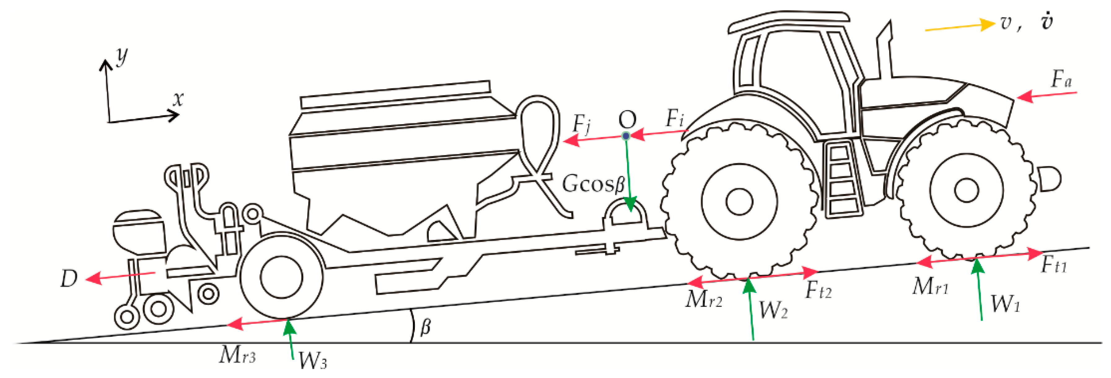
A schematic of the external forces applied to a four-wheel drive tractor with a precision planter is shown in Figure 2. The longitudinal dynamics of the tractor-planter combination unit on x-axis only could be considered when the cruise control or gear-shift schedule of straight driving is studied.
The longitudinal dynamic model is simplified to point-mass model as:
where Ft = Ft1 + Ft2 is the tractive force acting on the tractor’s driving wheels, Fi is the accelerating resistance, Fj is the force of slope resistance, Fa is the wind and air resistance, Mr is rolling resistance, D is the draft requirement for implement of precision planter.
These resistance forces can be calculated as follows:
where m is the mass of whole operating unit of the tractor with the precision planter (kg), v is the working speed of this unit (km/h), G is the gross weight of this unit (N), β is the slope of farmland (rad), CD is the coefficient of air resistance, A is the frontal area of tractor with planter (m2), f is the coefficient of rolling resistance.
The air resistance Fa can be neglected since the tractor-planter unit will be working on farmland with relatively low velocity while planting. The parameters of tyres and soil properties have significant effects on soil–traction interaction process [20]. Dwyer [21] present the equations of coefficient of rolling resistance as follows:
where W is the axle load (N), NCI is the mobility number, CI is the cone index (kPa), b is the tire section width (m), d is the overall tire diameter (m), δ is the tire deflection (m), h is the tire section height (m).
The draft force D is required to pull agricultural implements operated at shallow depths in horizontal direction of running, which is correlated to the width of implement and the speed at which it is pulled. The typical draft requirements can be calculated using the following equation [22]:
where Fx is a dimensionless soil texture adjustment parameter, C1, C2, C3 are machine-specific parameters, Ws is the seeding width (rows), Ts is the seeding depth (cm).
2.2. Powertrain Model
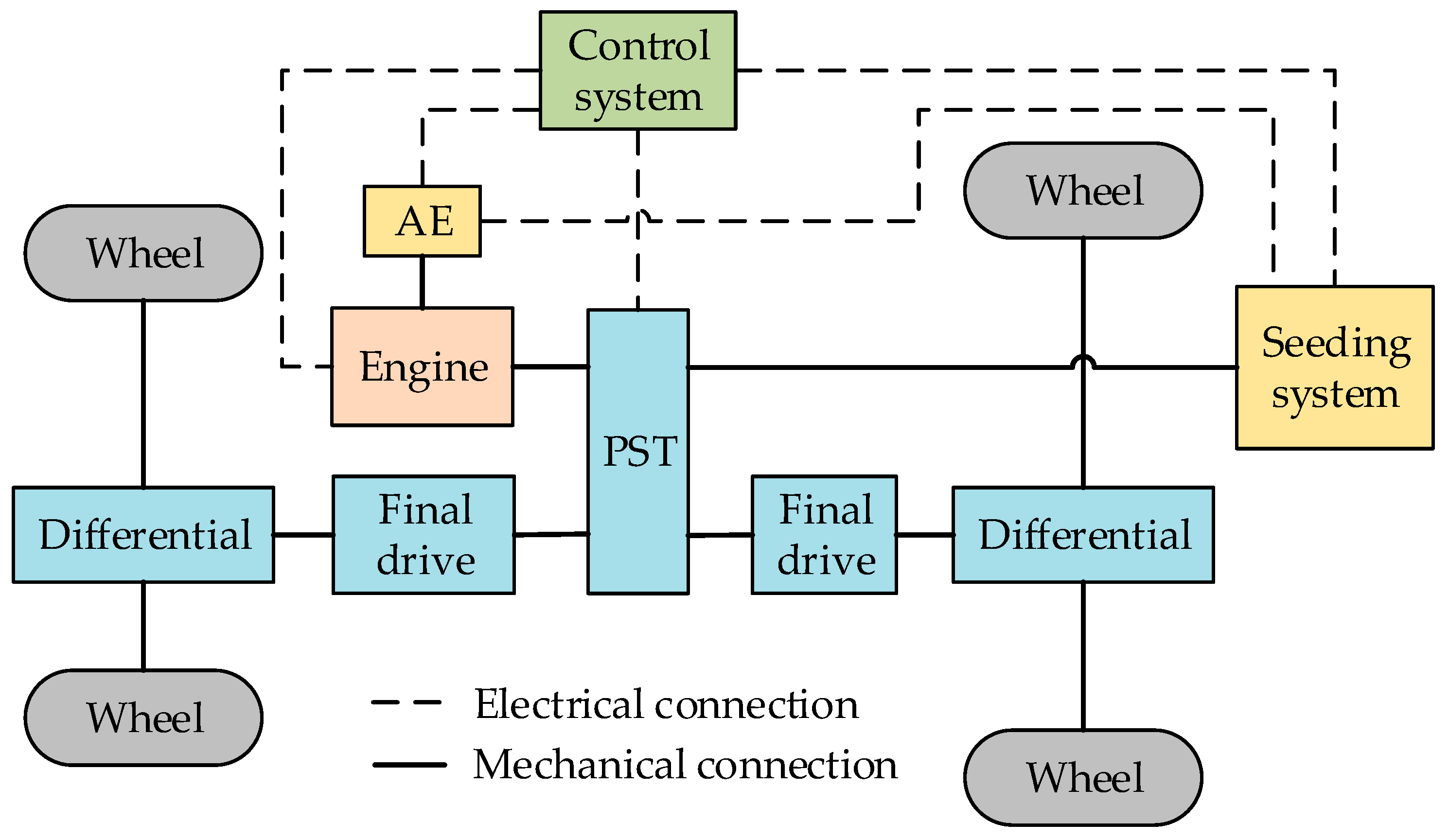
A multi-purpose tractor has a more complex powertrain than general road vehicles in order to match with different agricultural implements for various field operations. When the tractor works with a pneumatic planter, the engine of tractor supplies the energy to the propelling transmission system and seeding system, and also auxiliary equipment (AE) with little energy. It allows the tractor-planter combination operating unit to go forward or backward and to distribute seeds simultaneously while planting. A powertrain diagram of the operating unit is shown in Figure 3, which shows the routes of the mechanical and electrical connections. The mechanical power which reaches the seeding system from the power-shift transmission (PST) is transmitted through the power take-off (PTO) shaft.
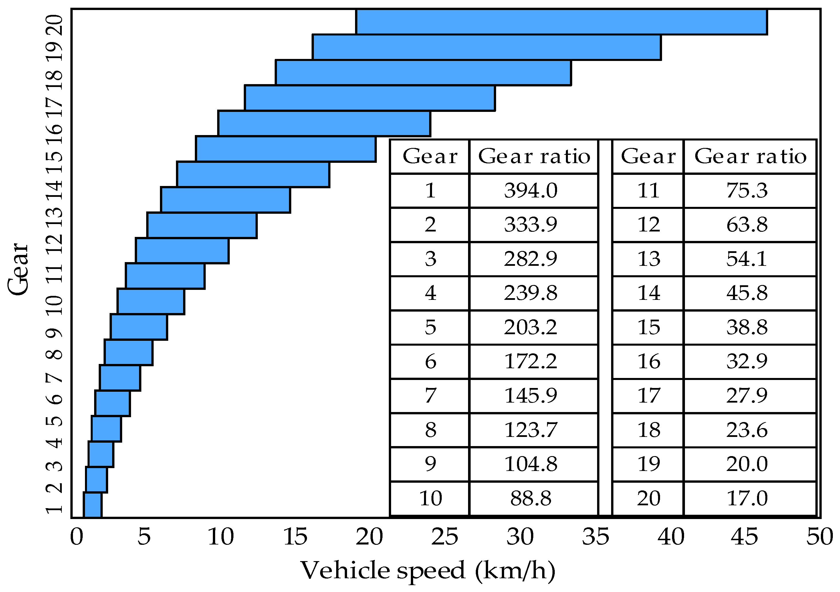
Based on a power-shift transmission proposed by New Holland [23], the transmission ratio parameters of a full power-shift transmission which has twenty forward gears are designed in this paper. The power-shift transmission allows the power to be transmitted continually by phasing the operation of the hydraulically actuated clutch packs into each other.
The theoretical travelling speeds of tractor installed with the full power-shift transmission in this paper are shown in Figure 4. In addition, the information of tractor’s total speed ratio of engine to rear drive axle (overall drivetrain) of each gear is presented in Figure 4.
The speed and torque can be calculated by:
where ne, nra, nPTO are the engine speed, rear axle speed and PTO shaft speed, respectively (rpm), ig, iPTO are total speed ratio of engine to rear drive axle and PTO shaft, respectively, r is rolling radius of rear wheels (m), s is the slip, Te, TAE, Tt, TPTO are the engine torque, torque of auxiliary equipment, torque of driving wheels, torque of PTO device, respectively (N·m), ηe1, ηe2 are mechanical efficiencies, Jx is the whole powertrain’s inertial moment which is converted into engine output shaft equivalent rotational inertia (kg·m2), ωe is angular velocity of engine (rad/s).
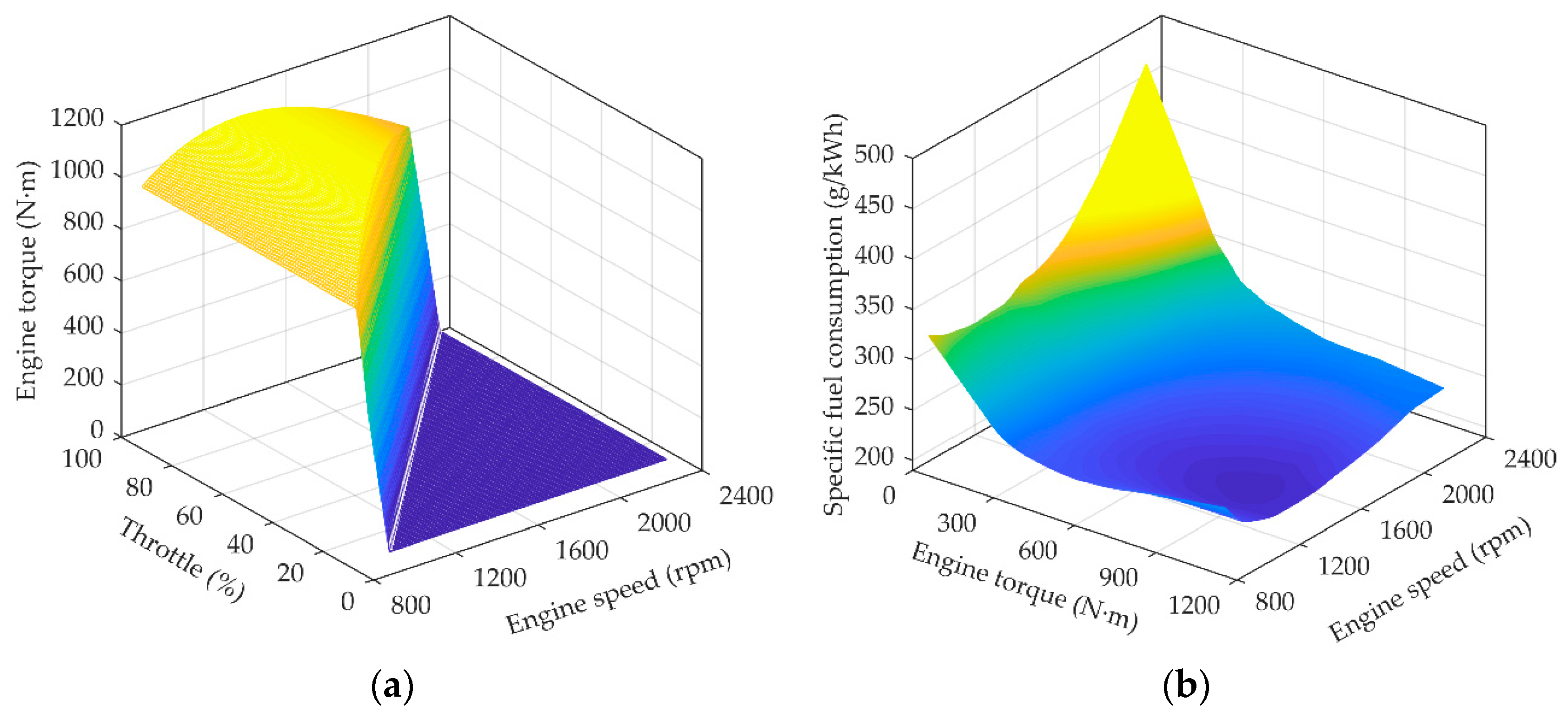
A diesel engine of 191 kW with the rated torque of 825 N·m at rated engine speed of 2200 rpm is selected as an example in this paper, with full range speed governing features. The engine torque and brake specific fuel consumption are nonlinear functions of many parameters. Written as Equations (12) and (13), the engine static torque can be considered as a function of engine speed and throttle opening, and brake specific fuel consumption can be considered as a function of engine speed and engine torque:
where a is engine throttle opening (%), be is brake specific fuel consumption (g/(kW·h)).
The static engine torque map and specific fuel consumption map which are from the engine test are shown in Figure 5.
In a simulation, the engine torque and fuel consumption can be obtained by the static engine torque map and brake specific fuel consumption map with interpolation. The dynamic engine torque model is formed by the static engine torque map with a subsequent first order inertial element.
In this paper, the gear shifting process is neglected, so the complex clutch model is simplified as a Boolean switch.
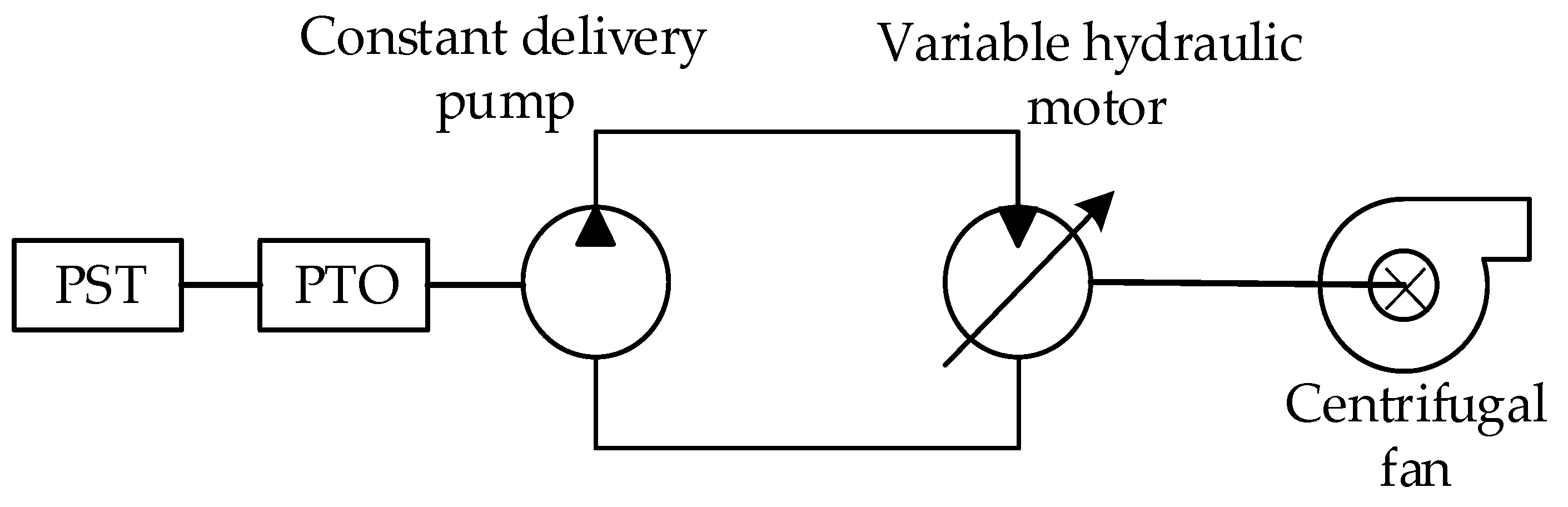
A pneumatic precision planter (also called air-suction type precision planter) is used in this study, which is suitable for precision seeding of field crops. The configuration of the power system for the centrifugal fan of the pneumatic precision planter is shown in Figure 6. It mainly consists of a centrifugal fan, constant delivery hydraulic pump driven by the PTO shaft from power-shift transmission of tractor, and a variable hydraulic motor whose displacement can be automatically regulated based on the operation requirements.
The centrifugal fan is used to transfer seeds to the discharge plate of the seed metering device for seed distribution. By controlling the displacement of the hydraulic pump automatically, a stable continuous suction pressure is maintained, which is beneficial to the planting quality. This power system can be simplified as Equations (14) and (15):
where Pp is the power of the constant delivery hydraulic pump (kW), p is working pressure of the hydraulic system (MPa), V is the displacement of the hydraulic pump (L/r), np is speed of the hydraulic pump (rpm), Tp is the torque of input shaft of hydraulic pump (N·m).
2.3. Seed Metering System Model
The performance of the seed metering device which is a key component of a precision planter, as it directly affects the uniformity of seed distribution. Due to the poor planting quality of conventional planters with ground wheels driving, the driving system using electric motor is adopted by some agricultural machinery companies [24].
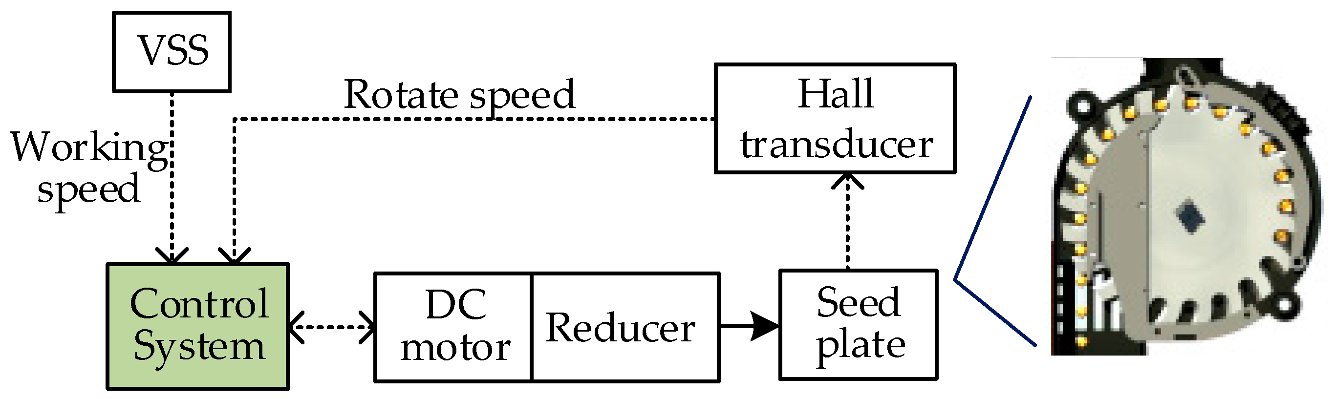
In order to maintain the consistent seed spacing at higher planting speeds, an electro-driving seed metering device is used in this paper, whose schematic is shown in Figure 7.
A brushless DC motor with permanent magnet is used as the actuator motor to adjust the speed of the seed plate. Moreover, the voltage balance and torque balance equations are written as Equations (16) and (17), respectively:
where Ua is the armature voltage (V), La is the armature inductance (H), Ia is the armature current (A), Ra is the armature resistance (Ω), Kb is a constant of proportionality, ωm is the rotor angular velocity of motor (rad/s), Tm is the motor torque (N·m). Jm is the rotor moment of inertia (kg·m2), Bm is the viscous friction coefficient, and Tl is the load torque of the DC motor (N·m).
The torque load Tl can be expressed by Equation (18):
where Tsp is the load torque of seed plate (N·m), Jsp is the moment of inertia of seed plate (kg·m2), ωsp is the angular velocity of seed plate (rad/s), imp is the transmission ratio of motor speed to seed plate speed.
According to the operating requirements, the target speed of DC motor can be calculated by Equation (19):
where nmr and npr are the speed requirements of drive motor and seed plate, respectively (rpm), Z is the set seed spacing (cm), H is the number of seed holes per plate.
The control system of the metering system regulates the input voltage of motor based on the difference between the demand speed and actual speed, which is monitored by the Hall Effect transducer to meet planting quality. The specific control strategy will be explained later.
3. Control Strategies
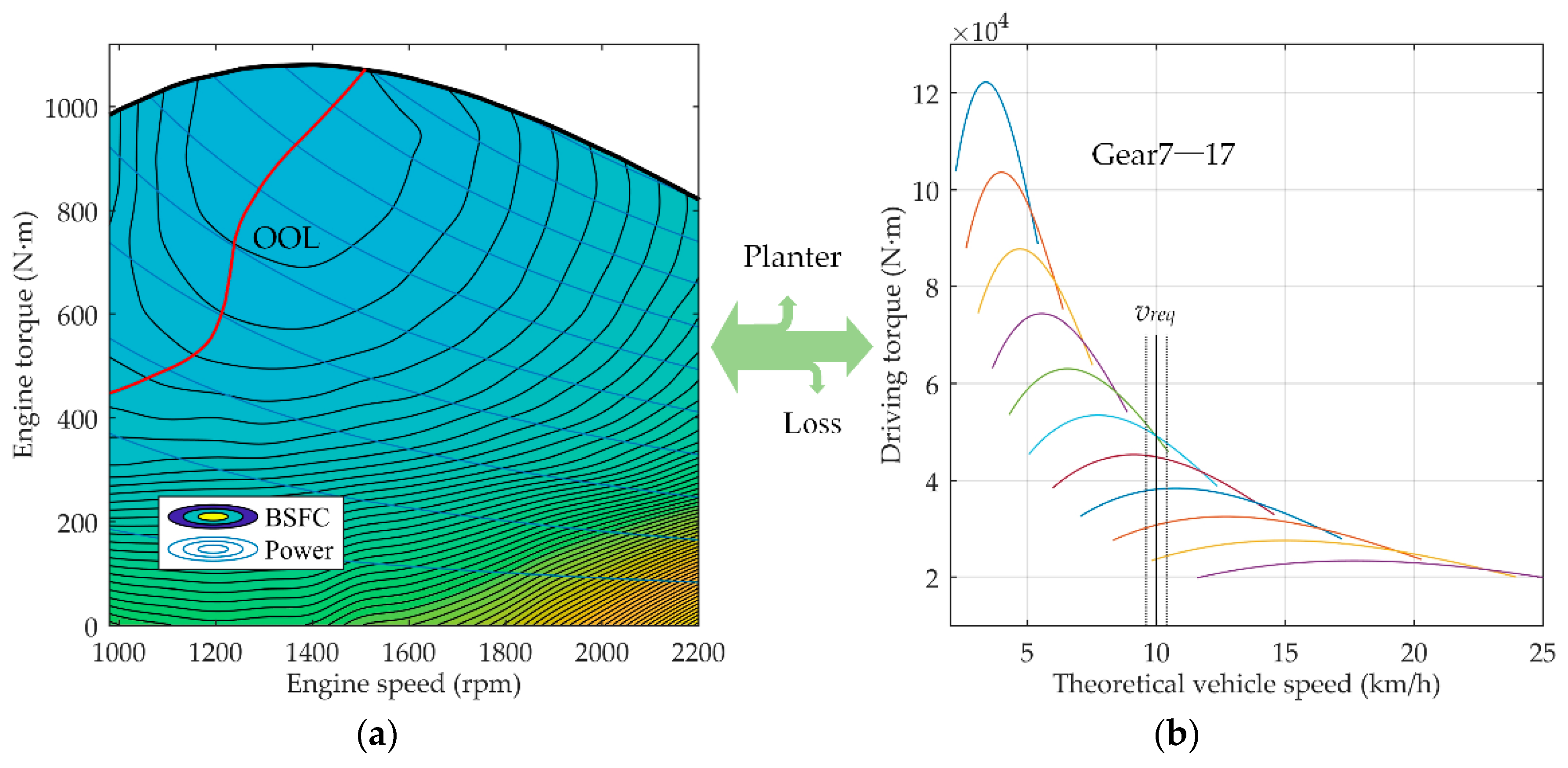
The universal performance map of a 191 kW diesel engine is presented in Figure 8a. The optimal operating line (OOL) marked as the red line is composed of the points with minimal value of brake special fuel consumption (BSFC) at each equipower line. The engine efficiency will achieve optimization by running the engine at optimal operating line under the demanded tractor power.
In a traditional cruise control system, an explicit target traveling speed is usually set by the driver, and then the control system regulates the powertrain to strictly meet the requirement of this target speed [7,11,12]. As the transmission ratio of stepped transmission is not continuous, the engine cannot always work at the optimal operating line under various conditions and travel speeds.
The tractors with power-shift transmission usually have many more gears than common vehicles, which provide advantages in fuel economy. Furthermore, the planting quality and work efficiency are of utmost importance in planting, and the planting speed precision does not need to be very accurate, which is acceptable within certain limits according to actual conditions.
Based on these characteristics of tractor and planting operation, a new cruise control strategy is proposed in order to improve the fuel economy of tractor-planter combinations in planting operations. The driver needs to set a reference target speed as an ideal planting speed and a certain range of deviations as an acceptable speed band. This target speed band instead of the traditional explicit target speed represents the driver’s demand in this paper. Under any working load within the speed range, the control system will automatically select the speed which has the optimal fuel efficiency which can make the working position of engine approach the optimal operating line. The cruise control discussed in this paper can be called economic cruise control.
When the tractor works under steady conditions, the torque of engine is used to supply the power for planter, accessories, also the rest of torque is used to drive the operating unit according to Equation (20). Figure 8b states the driving torques Tq at full throttle opening of gear 7 to gear 17, which are the gears suitable for planting operations. The black solid straight line and dotted lines represent the reference target speed vref (10 km/h) and the acceptable speed band, respectively. Within this speed band, a fuel-efficient speed can be achieved with a combination of engine speed and transmission gear at any given working load. The control system controls the tractor running at the most economical speed by adjusting the engine speed and shifting the gears of the tractor powertrain. Notice that the reference target speed vref (km/h) is the theoretical velocity, and it need to be converted by slip s and actual target planting speed vtar (km/h) based on Equation (21):
The part of engine torque TAE for accessories is considered as constant in this paper. Therefore, the correlation between driving torque and engine torque is confirmed when the parameters of planter and accessories are ensured under steady-state conditions.
In order to meet the needs of different drivers, listed in Table 1, four levels of speed deviation range are provided for four control modes in this paper. The driver can select a certain level as favor before planting and shift to different levels during planting. Theoretically, a higher level has better fuel economy.
The gear-shift schedule and engine speed regulating strategy are generated as follows.
3.1. Generation of Gear-Shift Schedule
During the planting operation under automatic speed control, the control systems determine which gear of the tractor transmission is selected and how the engine speed is adjusted based on the speed requirements, planting quality, and fuel economy. It is primary to meet the planting speed requirement of the driver and fuel economy while designing a gear-shift schedule. The seeding quality will be guaranteed by the control of the metering mechanism which will be discussed later.
In the studies on developing or optimizing economic gear-shift schedules for automobiles, Dynamic Programming (DP), as an algorithm for solving multi-stage decision processes, is a popular method used by scholars [25,26,27]. Prior knowledge of the drive cycle and loads is required when developing a gear-shift schedule by DP. However, as Equations (1)–(8) show, due to the diversities of soil properties, depth of seeding, farmland slope, etc., the external loads of a tractor-planter combination are difficult to determine in advance, so it is hard to generate a universal economic gear-shift schedule beforehand with common DP for a tractor in all working conditions when planting.
During a one-way planting process under cruise control, the speed changes less and the prepared seedbed is relatively smooth, and the load is relatively steady during planting. In this paper, the cost of fuel is used as the index to design a universal up-shift schedule for economic control strategies under different loads and speed requirements. Due to the features of cruise controlled planting with relatively steady speed and loads during one-way planting and in order to reduce computational cost, the fuel consumption during the processes of acceleration or deceleration when changing stages are neglected in this paper. Namely, the acceleration resistance is neglected while designing the up-shift schedule, so the DP method with stepwise reverse solving, as shown in Equation (22), is simplified to a method finding optimal decision for each stage (as expressed by Equation (23)):
where is Q is the fuel consumption in whole process (mL); N is the number of stages, Q(N), Q(k) are fuel consumption in stage N and k, respectively.
The up-shift schedules for these four levels of control mode need to be developed individually.
The determination of optimal gear-shift point is performed at each constant reference target operating speed, from 4.1 km/h to 18 km/h in steps of 0.1 km/h. At each constant reference target operating speed, the driving torque increases from 10,010 N·m to 80,000 N·m in steps of 10 N·m. The calculation will finish when the power of the engine reaches its maximum. Every change of torque is considered as one stage and every stage will maintain a travelling distance of 10 m. Within the target speed band limitations, the optimal transmission gears and optimal engine speeds are used to ensure a minimum fuel cost. The gear shifting conditions are recorded to generate up-shift maps.
The objective function is shown in Equation (23):
where Pe(k), be(k), v(k), Te(k), ne(k), Tq(k), ig(k) are engine power (kW), brake special fuel consumption (g/(kW·h)), planting speed (km/h), engine torque (N·m), engine speed (rpm), driving torque (N·m), total speed ratio in stage k, respectively, and Δd is travelling distance at each stage (m), ρ is the fuel density (kg/L).
The state space x(k) is shown by Equation (27):
where g(k) is the transmission gear in stage k.
The constraints on the driving torque, transmission gear, and engine speed are shown as Equations (28)–(30):
The driving torque and transmission gear are within the suitable range for planting. The engine speed is limited by the characteristics of the diesel engine used in this study. When the working torque of the engine approaches a maximum which is close to the engine full-load characteristic curves shown in Figure 8a, an undesired sharply increase of load may cause the tractor speed to decrease sharply or even stalling. Therefore, some extra torque needs to be kept in reserve to deal with sudden changes of load in designing the gear-shift schedule.
Thus the torque-constraining of engine is:
where Te,max is the maximum engine torque at real-time engine speed.
The state transitions are the changes of driving torque, gear and desired engine speed. The driving torque will increase by 10 N for every added stage. The transmission gear will up-shift, sustain, or down-shift when the stage is increasing. The desired engine speed is located within a range which is based on the target speed band:
In this paper, since the processes of acceleration and deceleration are neglected and the running distance of each stage is equal in designing the up-shift schedule for cruise control, as long as we can confirm the optimal solution J(k) for every stage, and the global optimum value for whole process can be ensured, so the total solution procedure is as follows:
- Let vref = 4.1;
- Let k = 1 and Tq(1) = 10010, calculate the optimal values of g(1) and ne(1) which guarantee J(1) = minQ(1);
- Let k = k + 1, determine appropriate x(k) under the object J(k) = minQ(k);
- Repeating the step 3 until k = N, then let vref = vref + 0.1;
- Repeating the steps 2–4 until vref = 18.
During this process, the moments of gear variation and corresponding conditions of reference target speed and driving torque are recorded, and the up-shift schedule maps can be generated by these previously summarized data. All the implementation of procedures are realized in Matlab 2017a (The MathWorks, Natick, MA, USA).
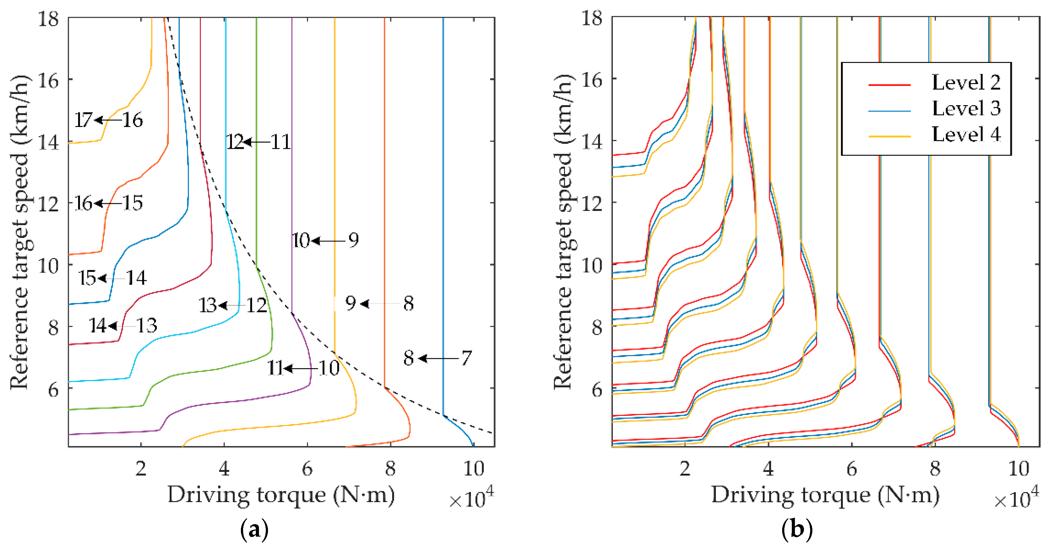
Figure 9a shows the up-shift schedule map for level 1 control mode, in which the ten curves from right to left represent the up-shift conditions of transmission gears from 7 to 16, respectively. The set reference target speed in the region beyond black dotted line is actually out of the capacity range of the engine, where the parts of up-shift lines are set as straight lines parallel to the y-axis. This means that when the reference target speed previously set by the driver exceeds the capacity of the engine in real driving conditions with the current load, the transmission gear is determined by the maximum speed which can be provided by the capacity of the engine, in order to avoid engine stalling.
The up-shift lines for control modes from level 2 to level 4 are shown in Figure 9b, which have a similar trend as level 1. There are slight differences in the up-shift lines at different levels, which indicate that the gear-shift conditions are slight different under these four levels control modes.
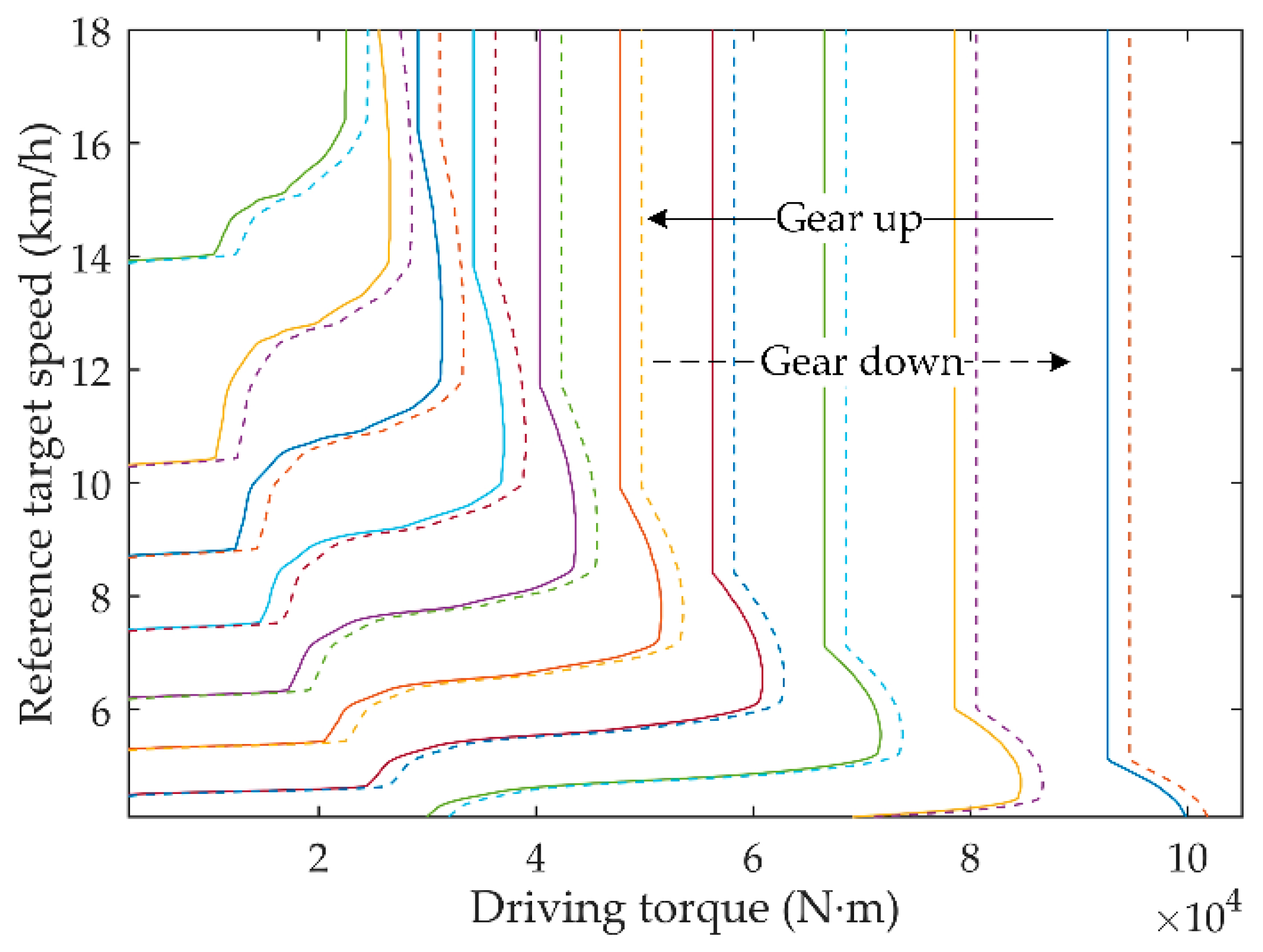
When two adjacent gear’s lines of up-shift and down-shift go to the same position, frequent gear shifting happens easily due to the fluctuation of load in the operating process, so a down-shift delay is adapted to solve this problem. In the gear-shift map, the down-shift curve is the up-shift curve with an upward offset of 1500 N·m, as the level 1 of control mode shows in Figure 10. The solid lines and dotted lines represent the up-shift and down-shift conditions, respectively. The situations of level 2–4 are similar, so the corresponding gear-shift maps are not shown in Figure 10.
In addition, due to the delay of the down-shift schedule, the driving torque may not meet the conditions of down shifting (according to the above discussion) when the torque of the engine climbs to full-load characteristic torque lines as the operating load is increasing, which may cause the engine to stall. Hence, down-shift schedule corrections have been established in this paper. It means that once the torque of engine reaches to 1050 N·m, which is slightly less than the maximum engine torque, a down-shift order is issued.
3.2. Cruise Control Strategy
In actual planting conditions, the operation process of a tractor can be divided into several stages as follows:
- Starting and transiting: In this stage, the tractor needs to start smoothly and accelerate quickly to around the target speed by manipulating clutches and transmission manually or automatically.
- Automatic cruise control: In this stage, the gear-shift and engine throttle are controlled by the control system based on the working load and speed demands.
- Stopping and turning: While reaching the edge of the field, the tractor needs to be quickly decelerated and change travel direction.
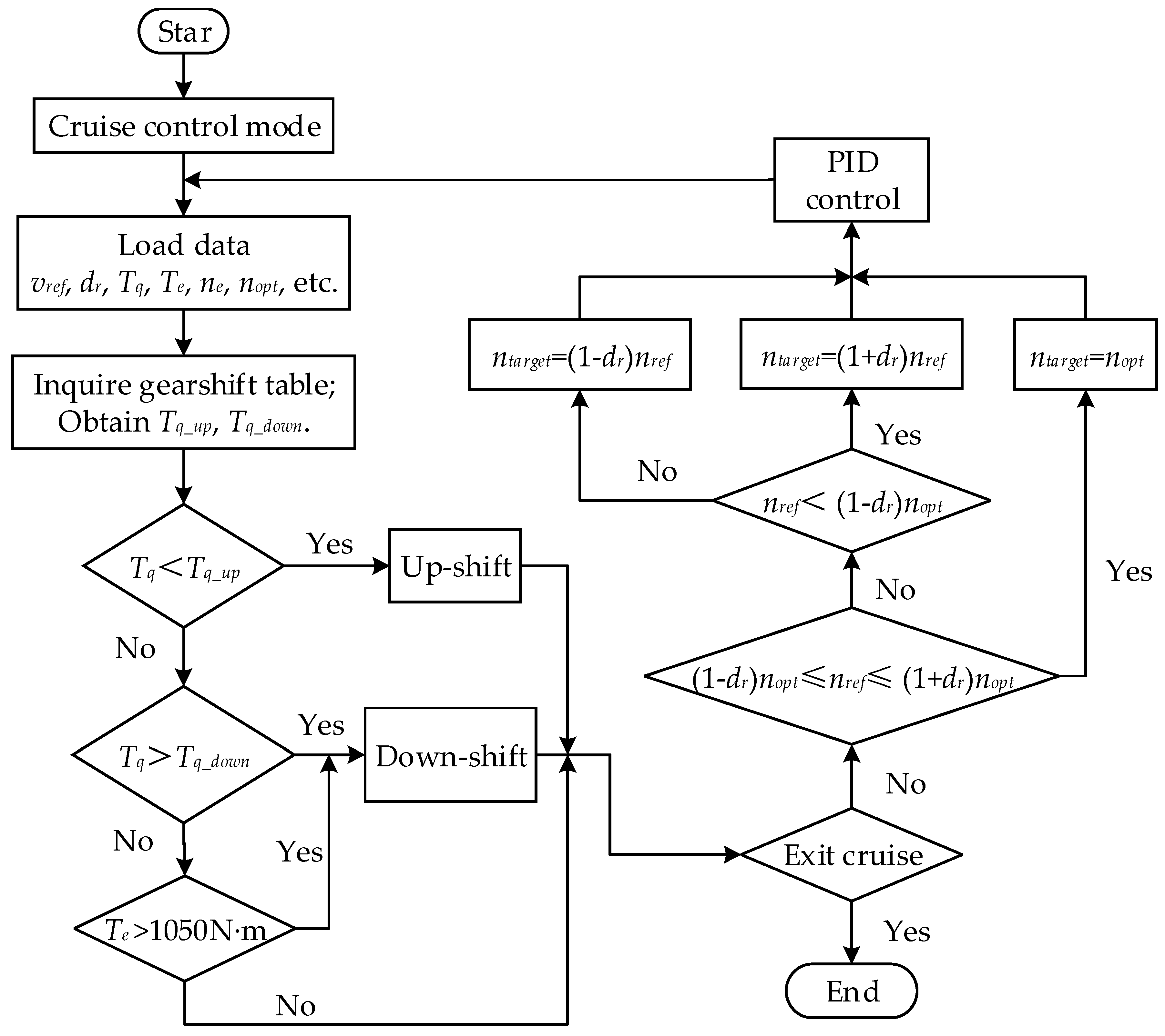
The automatic cruise control stage (the second stage) is the only focus in this paper, rather than the processes of starting and transiting, stopping and turning. The control flow chart of our cruise control strategy is shown in Figure 11. In practical operation, the real-time operation data is collected by the controller after starting cruise control mode. The driving torque Tq can be acquired by a torque sensor (if installed) or estimated by a resistance model or engine operating position. The transmission gear can be confirmed based on the gear-shift maps developed above. In order to meet the planting speed demands and fuel-efficiency purposes, the engine speed needs to be regulated.
The target engine speed is provided as calculated by Equations (35) and (36):
where nref is the reference target engine speed (rpm) which is converted by reference target planting speed vref (km/h) and current transmission ratio ig, nopt is the engine speed (rpm) on the OOL under real-time load.
PID control and fuzzy logic control are usually used in cruise control. As PID control is a simple and reliable algorithm, a closed-loop PID is used in this study to control the throttle opening of the engine to meet the target engine speed. A basic PID controller in continuous time and discrete controller are expressed by Equations (37) and (38), respectively [28]:
where a(t) is throttle opening, e(t) is the error between the target engine speed and actual engine speed, Kp, Ki and Kd are the proportional, integral, and differential gain constant, respectively. e(k) is the discrete error between the target engine speed and actual engine speed, a(k) is the discrete throttle opening, k is sampling points.
Additionally, the cruise control system will be suspended during the gear shifting process to avoid the conflict between the gear shifting process control and cruise control.
3.3. Control Strategy of Precision Seed Metering Device
The seed spacing and uniformity of seed distribution are the main indicators for evaluating planting quality. The seed spacing needs to be maintained around a set value while planting.
The speed of the tractor-planter combination will change within a small range under different operating loads by using our economy cruise control. Moreover, the speed will change significantly during the processes of starting, transiting and stopping. According to Equation (19), the target rotational speed of the seed plate and target speed of DC motor could be calculated and adjusted momentarily based on the change of the planting speed and some ideal seed spacing value.
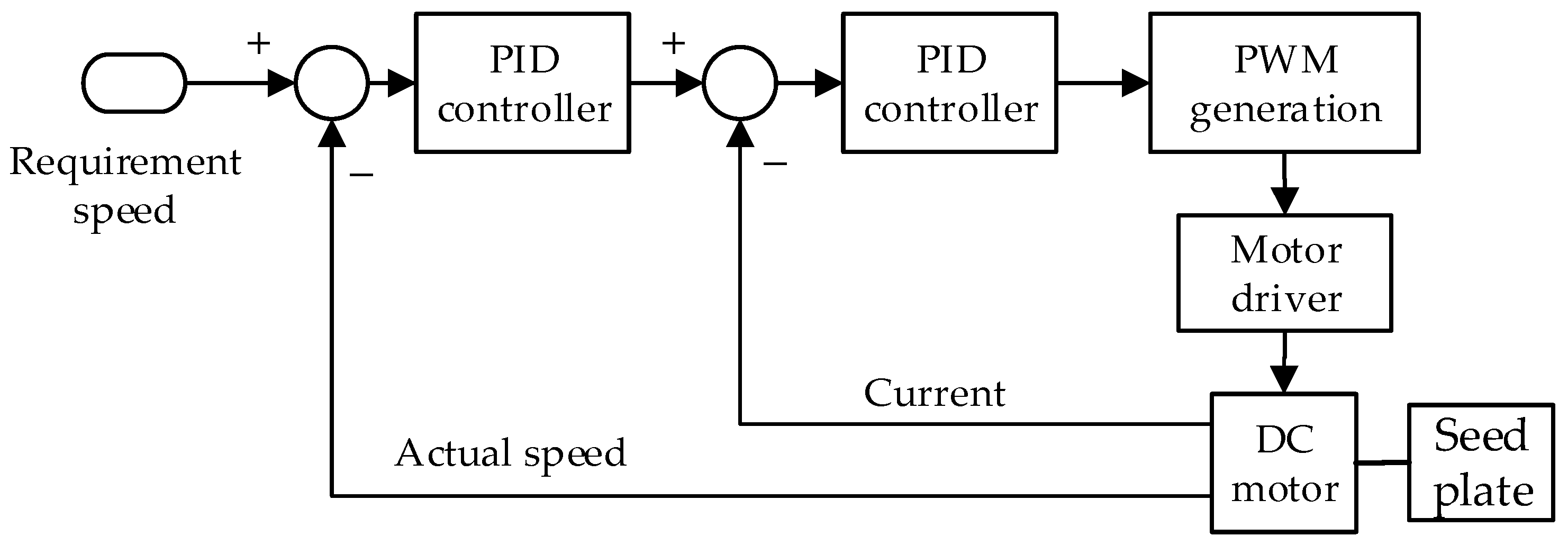
The Pulse Width Modulation (PWM) method is developed in this paper to adjust the motor voltage in order to regulate the DC motor speed. The control flow chart of the seed-metering device is shown in Figure 12. The speed and current double closed loop control is used in this system. The current loop and speed loop both adopt the PID controllers whose control principles are described above. The proportional, integral, and differential gain constant of the speed controller and current controller are set as Kp_n = 0.12, Ki_n = 0.33, Kd_n = 0, Kp_i = 0.8, Ki_i = 4.5, Kd_i = 0, respectively.
3.4. Simulation Method
In order to verify the economy and effectiveness of all the control strategies developed above for planting operations, it is essential to develop a simulation model that can simulate the behaviors of tractor-planter combination while planting. Based on the mathematical model, a simulation model of tractor-planter combination for planting operation is built with the Matlab/Simulink. This model includes modules for the engine, transmission, resistance, control system, and seed metering system and so on. The detailed process of engagement and separation of the clutches during gear shifting is ignored in this study. The control of transmission gear shifting of tractor for planting is performed by Matlab/Stateflow (The MathWorks, Natick, MA, USA). The basic parameters of the objective tractor are listed in Table 2. In order to simplify the model, the same specifications for the front and rear wheels of the tractor are assumed in this paper.
The parameters of the DC motor of the seed-metering device for driving the planter plate are listed in Table 3.
To verify the control strategies of road vehicles by simulation, some typical driving cycles have been established to simulate the real vehicle running status [29], such as Federal Test Program (FTP), Economic Commission for Europe (ECE), etc. but they are not suitable for field work. Some organizations, such as American Society of Agricultural and Biological Engineers (ASABE), and the German Agricultural Society, have proposed performance test standards for tractors [22]. However, these standards are focused on the performance tests of the tractor itself rather than the control strategy. Therefore, some simulation conditions are proposed in this paper to verify the proposed forward speed control strategies.
4. Results and Discussion
Four levels of cruise control mode are provided in this paper to meet the demands of different drivers. Level 1 allows no deviation from the reference target speed which is set by the driver. Level 2, level 3 and level 4 are similar in principle and only differ in the scopes of deviation, so the discussions of this paper focus on the results of simulations of level 1 and 2.
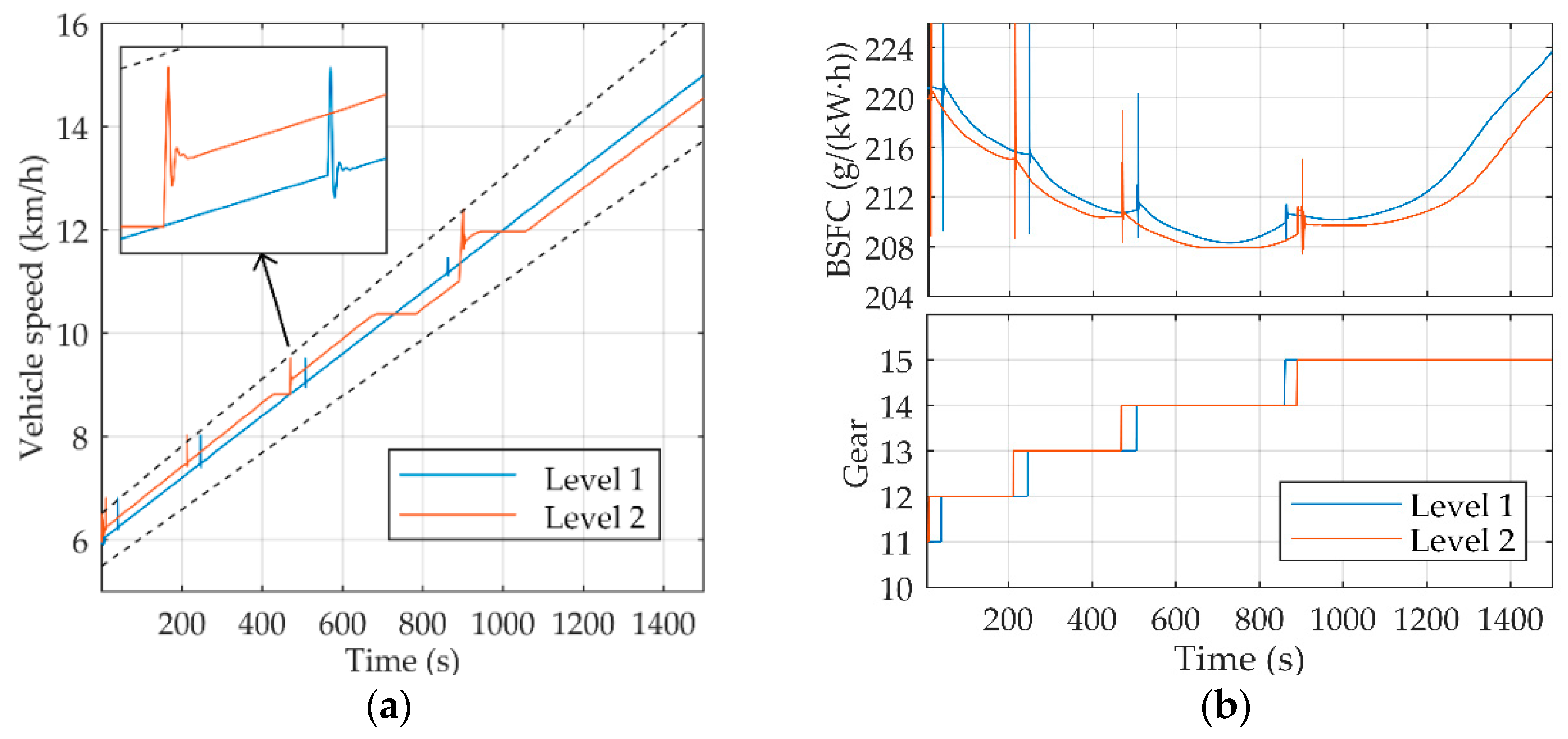
In order to test the effectiveness of our cruise control strategy, simulations of fixed running resistance and fixed reference target speed are given, respectively. In the fixed load simulation, the reference target speed changes evenly from 6 km/h to 15 km/h within 1500 s, and the total running resistance is set to be 40 kN as an assumption. The initial speed and gear are set as 6 km/h and gear 11, respectively. It is noticed that the driver won’t change the target speed so frequently and regularly in actual operation. The main purpose of this simulation is to prove the speed tracking accuracy under different cruise control modes.
The simulation results for speed are shown in Figure 13a. It shows that the running speed under level 1 mode can follow the reference target speed with high accuracy, except during the gear shifting process. The speed under level 2 mode has small non-uniform deviations with the ideal reference target speed. Figure 13b shows the situations of brake specific fuel consumption and transmission gears in these two levels. The moments of gear shifting have slightly differences, and the specific fuel consumption of level 2 is always no more than level 1’s. In short, the strategy of level 1 has better speed accuracy whilst the level 2 one has better fuel economy.
There is a dramatic change of the velocity curve and fuel consumption curve at each gear shifting. This is because Boolean switches are used to simulate clutches and the process of gear shifting is neglected in this paper. These shocks will be weakened or even eliminated if a reasonable control strategy is adopted for the gear shifting process.
In [7], the percentages of engine throttle opening less than 10% and more than 80% are set as the cruise control down-shift and up-shift thresholds for the tractor. The strategy mentioned in [7] is what we can call a current strategy which will be used to compare with the control strategies developed in this paper.
Figure 14 shows the simulation results by using level 1, level 2 and the current control strategies at a fixed reference target speed of 10 km/h. The running resistances include rolling resistance, draft resistance, slope resistance, etc., and all resistances are regarded as a whole working resistance in designing the operating conditions.
The first graph of Figure 14 shows the designed running resistance (external load) condition. The resistance is 47 kN initially and then reduces to 30 kN after 500 s gradually. From 600 s to 800 s, the resistance increases from 30 kN to 42 kN with a constant speed, and then the resistance fluctuates within certain limits until the end of the simulation. It should be noted that the load conditions in practical single-pass cruise operation could be much smaller than what has been designed previously.
The second graph in Figure 14 shows the speed variations under level 1, level 2 and current control strategies. These three strategies are all able to track the given reference target speed with various loads. The level 1 control strategy and the current strategy have higher accuracy in tracking the target speed than level 2.
The histories of gear, brake special fuel consumption, and engine speed are shown as the remaining graphs of Figure 14. At low load, the tractor operates in high gears with low fuel consumption, low engine speed and low power. The moments of gear shifting have differences between the two level modes and the current one. Obviously, the brake specific fuel consumption in level 2 control mode is lower than it in level 1, and they are both much lower than that of the current control strategy according to [7].
In sum, the economic cruise control strategies developed in this study can meet the requirements of cruise operation, and are consistent with predictions which indicate a better fuel economy in higher level control mode and better performance of tracking accuracy for speed in lower level control mode at the reference target speed.
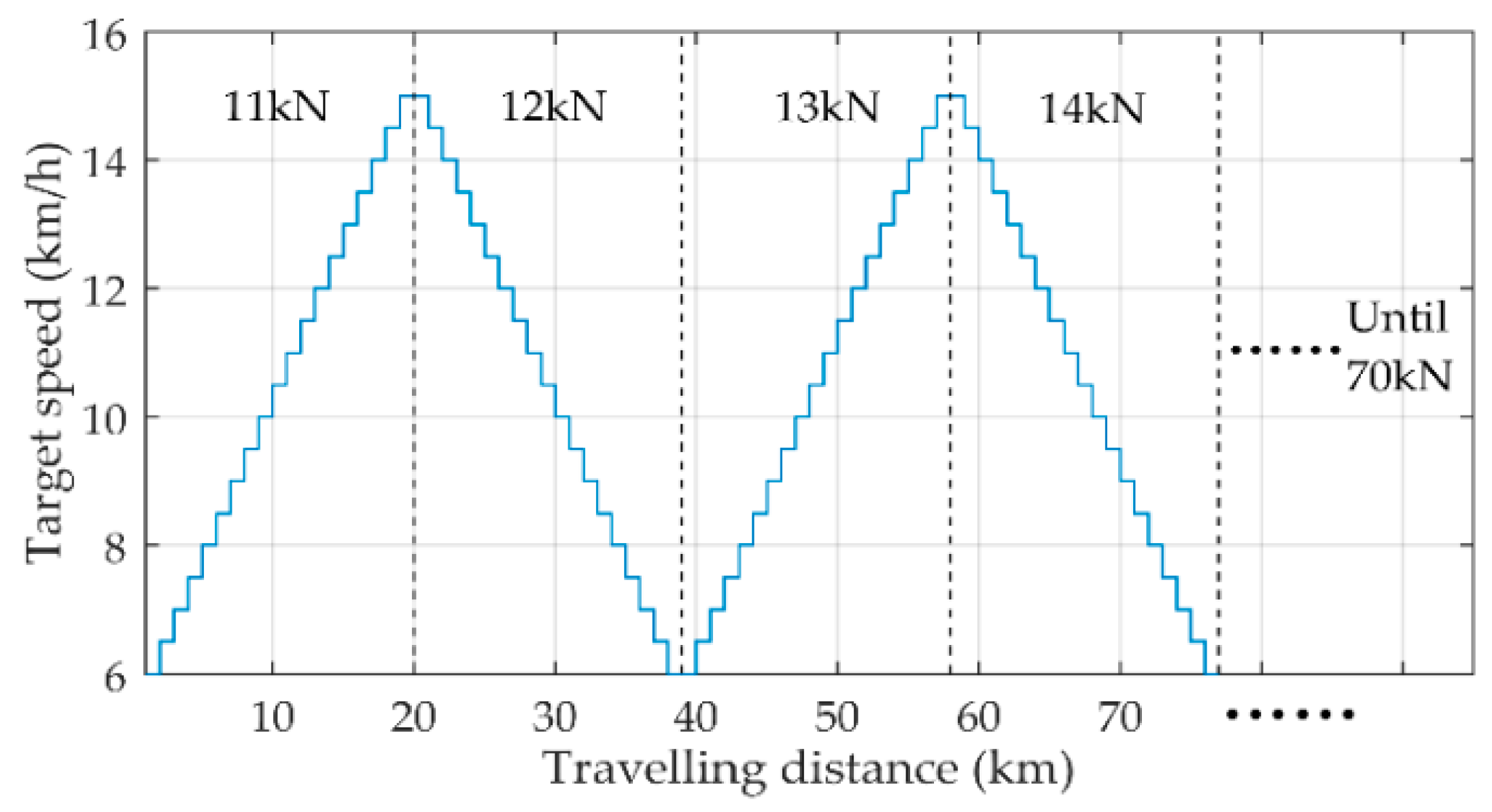
Nevertheless, it is difficult to explain the comprehensive fuel consumption and operation efficiency with a single constant load or constant target speed simulation. Different target speeds and loads need to be considered. As Figure 15 shows, working conditions combined with different loads and demand speed are designed for simulation to compare the fuel efficiencies of the different control strategies. The simulation process is as follows:
In this simulation, the traction resistance is set as 11 kN, the initial reference target speed is set as 6 km/h, and the tractor-planter combination is set to plant in cruise control mode. Once the travelled distance reaches 1 km, the target speed is increased by 0.5 km/h until it exceeds 15 km/h (if that can be achieved). Then the traction resistance increased by 1 kN. The target speed is decreased stepwise by 0.5 km/h until 6 km/h after every 1 km travelling distance. This process can be considered as one drive cycle. The cycles with different loads within 70 kN have been repeated. In addition, a fluctuating load of a sine wave with an amplitude of 800 N is given during the simulation. The simulation results are listed in Table 4.
Table 4 shows that the fuel consumptions using the economic cruise control strategies developed in this study are lower than those of the current strategy. The control modes from level 1 to level 4 have fuel economy improvements of 3.61%, 4.48%, 5.6% and 6.83% compared to the current strategy, respectively. This is mainly because the engine working positions with higher level control strategies are closer to the OOL on average than the lower level control strategy and current strategy.
The time consumed per kilometer under these strategies are similar. This means the planting productivities under comprehensive operation conditions with different control strategies are almost the same.
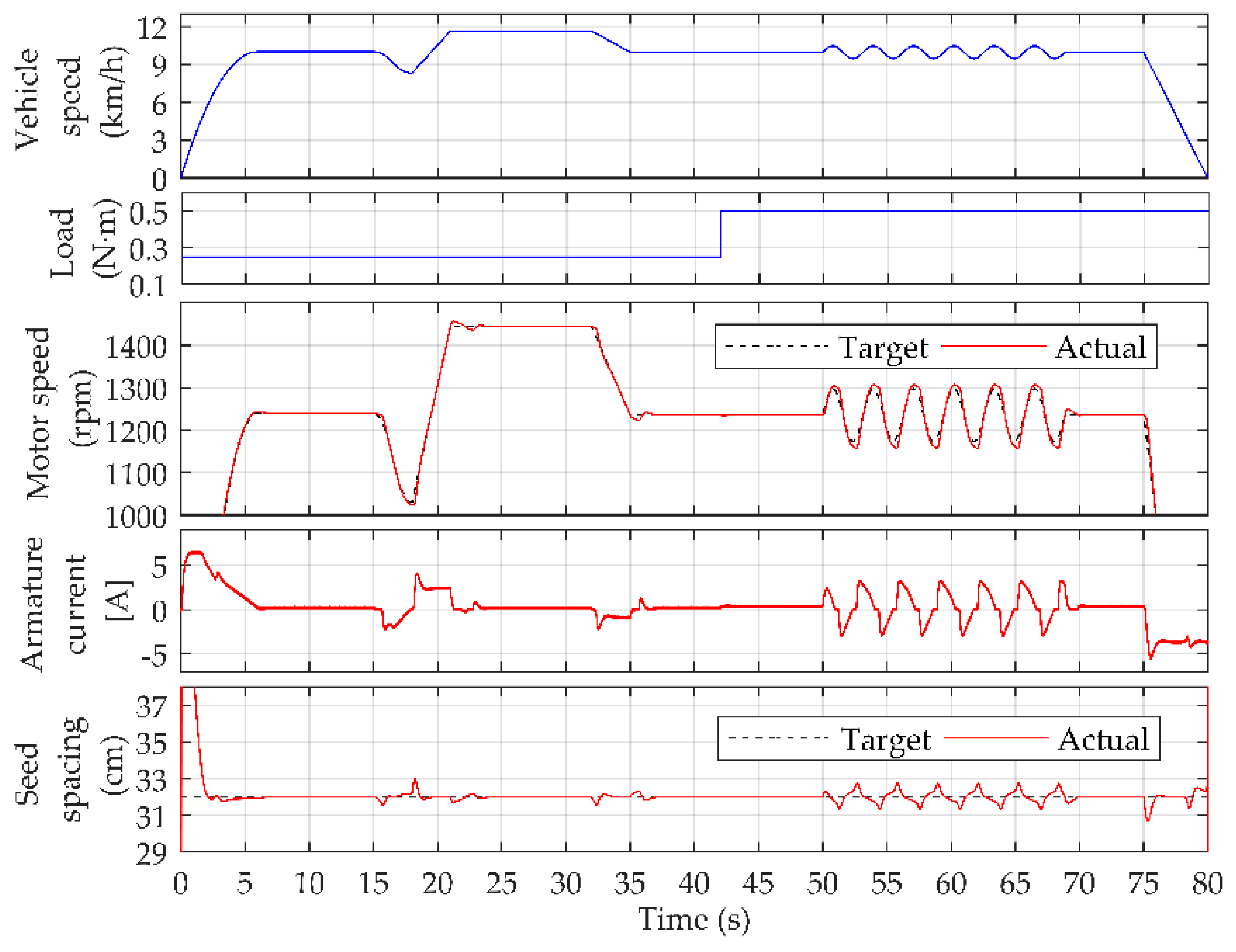
The operation process of the seed-metering device is simulated to verify the planting quality. The speed of tractor-planter combination in a single-pass operation like the curve in the first graph and the load of seed plate like the curve in the second graph are assumed in Figure 16.
Based on Equation (19), the target motor speed is shown by a black dotted line in the third graph of Figure 16. The simulation results show that the actual motor speed represented by the red solid line can track the target speed well. In this process, the armature current of driving motor is adjusted as the curve of the third graph in Figure 16.
The target seed spacing which is set as 32 cm and the simulated seed spacing are shown as the last graph in Figure 16. The seed spacing barely changes when the load of the seed plate changes. Although there are some fluctuations in the actual seed spacing when the tractor speed apparently changes, the fluctuation amplitude is less than 1 cm (3%) except for when the tractor is starting. This is able to meet the planting requirements well, and it means the planting quality can be guaranteed under the control methods in this study.
5. Conclusions
In this paper, an economic comprehensive control method is proposed for forward speed in planting. Based on mathematical models of the powertrain and operation characteristics, methods of generating a gear-shift schedule and regulating the planting speed are developed for cruise control in planting. Subsequently, in order to meet the requirements of different drivers or operation conditions, four levels economic control modes with different fuel economy performances are provided. In addition, a control strategy is developed for the motor of the seed-metering device to maintain the required seed spacing during planting, so as to ensure the planting quality. Finally, simulation models and simulation conditions are established to verify our proposed control strategies.
The simulation results show that the economic control strategies developed in this paper for forward speed can realize the function of cruise control that keep the operating speed around reference target speed set by the driver under fixed load or fixed target speed operation conditions. The brake special fuel consumption under the control strategies developed in this paper is lower than in the current strategy. The higher level control modes have better fuel efficiency with a larger speed deviation range than lower level control modes. The results obtained confirm our previous assumptions. Based on the simulation for testing comprehensive combined fuel consumption, the control modes from level 1 to level 4 have 3.61%, 4.48%, 5.6% and 6.83% fuel efficiency increments more than current method has, respectively. The combined productivity (time cost per kilometer) shows little difference. Furthermore, the simulation results also show that with the control method developed in this paper, the planting quality can be guaranteed (the error of seed spacing is within 3%) when the velocity changes during planting operations.
Acknowledgments
The authors acknowledge the financial support from the National Key Research & Development Program of China (No. 2016YFD0701100) and the Natural Science Foundation of China (No. 51375505).
Author Contributions
Baogang Li developed the control strategies and wrote the paper; Dongye Sun built the mathematical models; Minghui Hu produced the Matlab/Simulink program; Junlong Liu conceived the structure and research direction of the paper. All authors examined and approved the final manuscript.
Conflicts of Interest
The authors declare no conflict of interest.
References
- McBratney, A.; Whelan, B.; Ancev, T.; Bouma, J. Future directions of precision agriculture. Precis. Agric. 2005, 6, 7–23. [Google Scholar] [CrossRef]
- Li, M.; Imou, K.; Wakabayashi, K.; Yokoyama, S. Review of research on agricultural vehicle autonomous guidance. Int. J. Agric. Biol. Eng. 2009, 2, 1–16. [Google Scholar] [CrossRef]
- Backman, J.; Oksanen, T.; Visala, A. Navigation system for agricultural machines: Nonlinear model predictive path tracking. Comput. Electron. Agric. 2012, 82, 32–43. [Google Scholar] [CrossRef]
- Derrick, J.B.; Bevly, D.M. Adaptive steering control of a farm tractor with varying yaw rate properties. J. Field Robot. 2009, 26, 519–536. [Google Scholar] [CrossRef]
- Li, Y.; Efatmaneshnik, M.; Dempster, A.G. Attitude determination by integration of MEMS inertial sensors and GPS for autonomous agriculture applications. GPS Solut. 2012, 16, 41–52. [Google Scholar] [CrossRef]
- Pérez-Ruiz, M.; Carballido, J.; Agüera, J.; Gil, J.A. Assessing GNSS correction signals for assisted guidance systems in agricultural vehicles. Precis. Agric. 2011, 12, 639–652. [Google Scholar] [CrossRef]
- Han, K.; Zhu, Z.; Mao, E.; Song, Z.; Hu, F.; Xu, L. Cruise control system of tractor based on automated mechanical transmission. Trans. Chin. Soc. Agric. Eng. 2012, 28, 21–26. (In Chinese) [Google Scholar] [CrossRef]
- Marsden, G.; McDonald, M.; Brackstone, M. Towards an understanding of adaptive cruise control. Transp. Res. C Emerg. Technol. 2001, 9, 33–51. [Google Scholar] [CrossRef]
- Milanes, V.; Shladover, S.E.; Spring, J.; Nowakowski, C.; Kawazoe, H.; Nakamura, M. Cooperative adaptive cruise control in real traffic situations. IEEE Trans. Intell. Transp. Syst. 2014, 15, 296–305. [Google Scholar] [CrossRef]
- Moon, S.; Moon, I.; Yi, K. Design, tuning, and evaluation of a full-range adaptive cruise control system with collision avoidance. Control Eng. Pract. 2009, 17, 442–455. [Google Scholar] [CrossRef]
- Coen, T.; Saeys, W.; Missotten, B.; De Baerdemaeker, J. Cruise control on a combine harvester using model-based predictive control. Biosyst. Eng. 2008, 99, 47–55. [Google Scholar] [CrossRef]
- Coen, T.; Anthonis, J.; De Baerdemaeker, J. Cruise control using model predictive control with constraints. Comput. Electron. Agric. 2008, 63, 227–236. [Google Scholar] [CrossRef]
- Chen, J.; Ning, X.; Li, Y.; Yang, G.; Wu, P.; Chen, S. A fuzzy control strategy for the forward speed of a combine harvester based on KDD. Appl. Eng. Agric. 2017, 33, 15–22. [Google Scholar] [CrossRef]
- Na, G.; Jingtao, H. Variable universe adaptive fuzzy-PID control of traveling speed for rice transplanter. Trans. Chin. Soc. Agric. Mach. 2013, 44, 245–251. (In Chinese) [Google Scholar] [CrossRef]
- Grzesikiewicz, W.; Knap, L.; Makowski, M.; Pokorski, J. Study of the Energy Conversion Process in the Electro-Hydrostatic Drive of a Vehicle. Energies 2018, 11, 348. [Google Scholar] [CrossRef]
- Karbaschian, M.A.; Soeffker, D. Review and Comparison of Power Management Approaches for Hybrid Vehicles with Focus on Hydraulic Drives. Energies 2014, 7, 3512–3536. [Google Scholar] [CrossRef]
- Wang, J.; Lei, Y.; Ge, A.; Lu, X. Shift Strategy Research on Off-Road Vehicle; Technical Report; SAE International: Warrendale, PA, USA. [CrossRef]
- Yang, W.; Wu, G.; Dang, J. Research and Development of Automatic Transmission Electronic Control System. In Proceedings of the 2007 IEEE International Conference on Integration Technology, Las Vegas, NV, USA, 13–15 August 2007. [Google Scholar]
- Shen, W.; Yu, H.; Hu, Y.; Xi, J. Optimization of Shift Schedule for Hybrid Electric Vehicle with Automated Manual Transmission. Energies 2016, 9, 220. [Google Scholar] [CrossRef] [Green Version]
- Zoz, F.M.; Grisso, R.D. Traction and tractor performance. In Proceedings of the 2003 Agricultural Equipment Technology Conference, Louisville, KY, USA, 9–11 February 2003. [Google Scholar]
- Dwyer, M.J. The tractive performance of wheeled vehicles. J. Terramech. 1984, 21, 19–34. [Google Scholar] [CrossRef]
- ASABE Standards. Available online: http://elibrary.asabe.org/standards.asp (accessed on 15 January 2018).
- Molari, G.; Sedoni, E. Experimental evaluation of power losses in a power-shift agricultural tractor transmission. Biosyst. Eng. 2008, 100, 177–183. [Google Scholar] [CrossRef]
- Zhai, J.; Xia, J.; Zhou, Y.; Zhang, S. Design and experimental study of the control system for precision seed-metering device. Int. J. Agric. Biol. Eng. 2014, 7, 13–18. [Google Scholar] [CrossRef]
- Lei, Y.; Fu, Y.; Liu, K.; Li, X.; Liu, Z.; Zhang, Y.; Fu, X. Research on Optimal Gearshift Strategy for Stepped Automatic Transmission Based on Vehicle Power Demand; Technical Report; SAE International: Warrendale, PA, USA, 2017. [Google Scholar] [CrossRef]
- Baglione, M.; Duty, M.; Ni, J.; Assanis, D. Reverse dynamic optimization methodology for maximizing powertrain system efficiency. IFAC Proc. Vol. 2007, 40, 17–24. [Google Scholar] [CrossRef]
- Ngo, D.V.; Hofman, T.; Steinbuch, M.; Serrarens, A.; Merkx, L. Improvement of fuel economy in Power-Shift Automated Manual Transmission through shift strategy optimization—An experimental study. In Proceedings of the 2010 IEEE Vehicle Power and Propulsion Conference, Lille, France, 1–3 September 2010. [Google Scholar]
- Ang, K.H.; Chong, G.; Li, Y. PID control system analysis, design, and technology. IEEE Trans. Control Syst. Technol. 2005, 13, 559–576. [Google Scholar] [CrossRef]
- Emission Test Cycles. Available online: https://www.dieselnet.com/standards/cycles/index.php (accessed on 15 January 2018).
Figure 1.
Tractor-planter combination in planting operation.

Figure 2.
Schematic of external forces acting on tractor-planter combination unit.

Figure 3.
Powertrain diagram of tractor-planter combination operating unit.

Figure 4.
Travelling speed range versus speed ratios of overall drivetrain of different gears.

Figure 5.
Engine characteristics maps. (a) Engine torque; (b) Brake specific fuel consumption.

Figure 6.
The configuration of power system for centrifugal fan of pneumatic planter.

Figure 7.
Schematic of seed metering device.

Figure 8.
(a) Engine universal performance; (b) Tractor driving torque.

Figure 9.
The up gear-shift maps. (a) Mode of level 1; (b) Modes of level 2–4.

Figure 10.
The static gear-shift map for control mode of level 1.

Figure 11.
Control flow of cruise control.

Figure 12.
Control structure of the seed metering device.

Figure 13.
Simulation results of fixed load. (a) Speed variations; (b) Variations of brake specific fuel consumption and transmission gear.
Figure 13.
Simulation results of fixed load. (a) Speed variations; (b) Variations of brake specific fuel consumption and transmission gear.

Figure 14.
Simulation results of constant reference target speed.
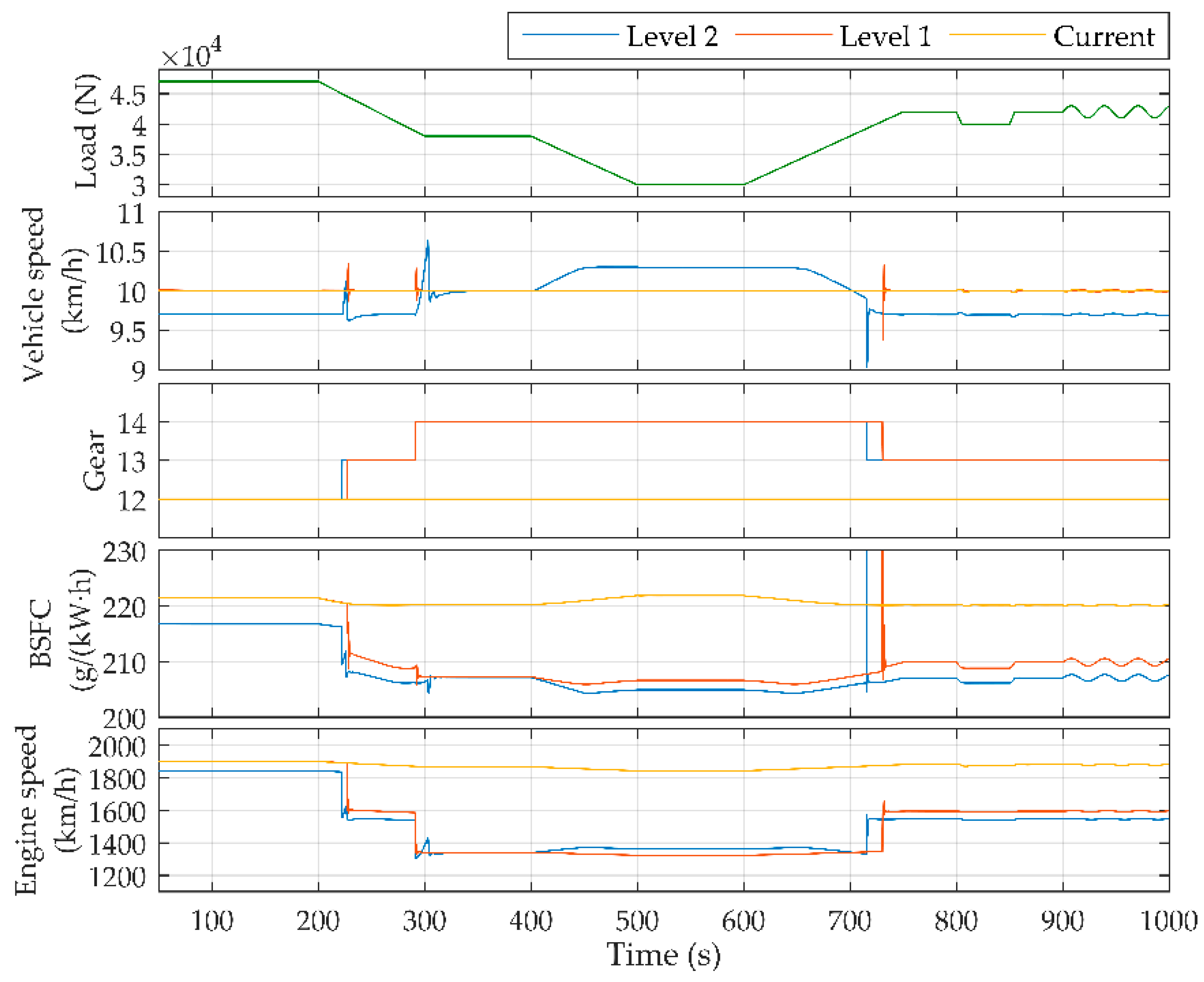
Figure 15.
Travelling cycles for simulation.

Figure 16.
Simulation results for seed spacing.


Table 1.
Speed deviation range.
| Mode | Maximum Deviation Proportion dr | Target Speed Band |
|---|---|---|
| Level 1 | 0% | [vref, vref] |
| Level 2 | 3% | [0.97vref, 1.03vref] |
| Level 3 | 6% | [0.94vref, 1.06vref] |
| Level 4 | 9% | [0.91vref, 1.09vref] |
Table 2.
Basic parameters of the objective tractor.
| Parameters | Value |
|---|---|
| Rated power of engine (kW) | 191 |
| Rolling radius of wheels (m) | 0.95 |
| Mass of tractor with counter weight (kg) | 11,000 |
| Mechanical efficiency of drive system ηm1 | 0.87 |
| Mechanical efficiency of PTO ηm2 | 0.97 |
Table 3.
Parameters of DC motor of seed-metering device.
| Parameters | Value |
|---|---|
| Rated speed (rpm) | 3000 |
| Maximum speed (rpm) | 4000 |
| Rated power (W) | 60 |
| Rated voltage (V) | 12 |
| Rated current (A) | 3.28 |
| Maximum current (A) | 6.56 |
| Rated torque (N·m) | 0.192 |
Table 4.
Comparison of fuel efficiency and average time.
| Control Mode | Mean Fuel Consumption (L/km) | Mean Time (s/km) |
|---|---|---|
| Current | 2.768 | 411.4 |
| Level 1 | 2.668 | 410.8 |
| Level 2 | 2.644 | 414.1 |
| Level 3 | 2.613 | 417.9 |
| Level 4 | 2.579 | 421.7 |
© 2018 by the authors. Licensee MDPI, Basel, Switzerland. This article is an open access article distributed under the terms and conditions of the Creative Commons Attribution (CC BY) license (http://creativecommons.org/licenses/by/4.0/).
Share and Cite
MDPI and ACS Style
Li, B.; Sun, D.; Hu, M.; Liu, J. Research on Economic Comprehensive Control Strategies of Tractor-Planter Combinations in Planting, Including Gear-Shift and Cruise Control. Energies 2018, 11, 686. https://doi.org/10.3390/en11030686
AMA Style
Li B, Sun D, Hu M, Liu J. Research on Economic Comprehensive Control Strategies of Tractor-Planter Combinations in Planting, Including Gear-Shift and Cruise Control. Energies. 2018; 11(3):686. https://doi.org/10.3390/en11030686
Chicago/Turabian StyleLi, Baogang, Dongye Sun, Minghui Hu, and Junlong Liu. 2018. "Research on Economic Comprehensive Control Strategies of Tractor-Planter Combinations in Planting, Including Gear-Shift and Cruise Control" Energies 11, no. 3: 686. https://doi.org/10.3390/en11030686
Note that from the first issue of 2016, this journal uses article numbers instead of page numbers. See further details here.