Experimental and Numerical Analyses of the Sloshing in a Fuel Tank
by
 , , ,
, , ,
Emma Frosina
1,* ,
,
Adolfo Senatore
1 ,
,
Assunta Andreozzi
1 ,
,
Francesco Fortunato
2 and
Pino Giliberti
2 1
Department of Industrial Engineering, University of Naples Federico II, Via Claudio, 21-80125 Naples, Italy
2
Fiat Chrysler Automobiles (F.C.A.), Via Ex Aeroporto-80038, Pomigliano d’Arco, 21-80125 Naples, Italy
*
Author to whom correspondence should be addressed.
Energies 2018, 11(3), 682; https://doi.org/10.3390/en11030682
Submission received: 31 January 2018
/
Revised: 8 March 2018
/
Accepted: 15 March 2018
/
Published: 17 March 2018
Abstract
:The sloshing of fuel inside the tank is an important issue in aerospace and automotive applications. This phenomenon, in fact, can cause various issues related to vehicle stability and safety, to component fatigue, audible noise, vibrations and to the level measurement of the fuel itself. The sloshing phenomenon can be defined as a highly nonlinear oscillatory movement of the free-surface of liquid inside a container, such as a fuel tank, under the effect of continuous or instantaneous forces. This paper is the result of a research collaboration between the Industrial Engineering Department of the University of Naples “Federico II” and the R&D department of Fiat Chrysler Automobiles (F.C.A.) The activity is focused on the study of the sloshing in the fuel tank of vehicles. The goal is the optimization of the tank geometry in order to allow, for example, the correct fuel suction under all driving conditions and to prevent undesired noise and vibrations. This paper shows results obtained on a reference tank filled by water tinted with a dark blue food colorant. The geometry has been tested on a test bench designed by Moog Inc. on specification from Fiat Chrysler Automobiles with harmonic excitation of a 2D tank slice along one degree of freedom. The test bench consists of a hexapod with six independent actuators connecting the base to the top platform, allowing all six Degrees of Freedom (DOFs). On the top platform there are other two additional actuators to extend pitch and roll envelope, thus the name of “8-DOF bench”. The designed tank has been studied with a three-dimensional Computational Fluid Dynamics (CFD) modeling approach, too. By the end, the numerical and experimental data have been compared with a post-processing analysis by means of Matlab® software. For this reason, the images have been reduced in two dimensions. In particular, the percentage gaps of the free surfaces and the center of gravity have been compared each other. The comparison, for the three different levels of liquid tested, has shown a good agreement with a discrepancy always less than 3%.
1. Introduction
Nowadays the sloshing of fuel inside the tank of vehicles is a very important research issue. Many studies have been done in order to find a methodology able to predict the oscillation of the liquid inside the tank. As is well known, the sloshing phenomenon can be defined as the motion of the free surface of a liquid in a partially filled tank. The fluid motion is due to external forces and to the interaction with the gas phase. Consequently, the effects of sloshing on the containers are noise, inertial loads and structural vibrations and potentially is can also have effects on the stability of the vehicle [1]. The relevance of the implications on the vehicle depends on several aspects. First of all, it depends on the type of motion, the amplitude and the frequency of excitation, but also on the geometrical aspects like the tank geometry, the fill levels and the liquid properties. The motion of the vehicle during the travelling is another important aspect that has to be taken into account in the sloshing analysis because with high acceleration, cornering and braking fluid inside the tank is forced to move. However, the prediction models need to include the interaction between the liquid and the gas by integrating multiphase applications.
In this paper the sloshing is analyzed looking in particular at fuel tanks, but this phenomenon is observed and studied for the all vehicle containers. The proposed numerical methodology can be applied to study sloshing in all the tanks inside a car. It has been observed that, in automotive applications, the sloshing does not affect the vehicle stability during travel; however, it may cause, as said, unwanted acoustic noise issues in the passenger compartment, structural vibrations, problems with low fluid (fuel, oil, water, etc.) level management and vapor emissions. Therefore, the individuation of a robust numerical model able to predict the free surface motion of a liquid is of great interest to the scientific community. For this reason, many researchers have investigated sloshing phenomena with modeling and experimental approaches.
Experimental analysis has been carried out by Pal et al. [2] to study the sloshing in a cylindrical container with and without baffles. Aus der Wiesche [3] also studied the sloshing in automotive fuel tanks experimentally, analyzing in particular the noise deriving from the phenomenon. He established a correlation between the simulated pressure fluctuations and the recorded slosh noise within the sloshing liquid. Abramson [4] and Ibrahim [5] have also analyzed the sloshing using both experimental and modeling techniques for different containers shapes.
Numerical models have been investigated by Liu and Lin [6] and Popov et al. [7]. In particular, Liu and Lin [6] analyzed a nonlinear liquid sloshing with broken free surfaces while Popov et al. [7] investigated the effect on the fluid motion of curvature and acceleration in rectangular containers. They observed that the most intense sloshing occurs when the fill level is approximately 30–60%. Ubbink [8] developed an accurate Computational Fluid Dynamics (CFD) methodology able to predict the flow behavior of immiscible fluids. Fluids (water and air) are separated by a well-defined interface and are subject to an external solicitation to reply to a vehicle’s movement on a bend. The choice of the water instead of gasoline/diesel is strategic because of the safety, the simplicity of disposal and the unlimited availability at no cost. However, in the future the same Experimental Fluid Dynamics (EFD) and Computational Fluid Dynamics (CFD) analyses will be performed with fuels.
Even if the study concerns the analysis of the fluid dynamics of two immiscible fluids, it considers the strong cohesion forces between their molecules. In fact, when fluids are miscible, the study can be approached considering the surface tension (resistance to mixing). A negative value of the surface tension indicates no resistance to mixing, as underlined by Batchelor [9]. As well known, the flow behavior of immiscible fluids depends on chemical reactions or phase changes due to high temperatures.
The flow of immiscible fluids can be classified into three groups based on the interfacial structures and topographical distributions of the phases, namely segregated flows, transitional or mixed flows and dispersed flows [10]. The classification is explained by considering a closed tank-filled with a liquid and a gas. The container is forced to oscillate with low amplitudes and frequencies. The sloshing in this case falls in the first class where two phases remain separated with a single well-defined interface. If the frequency and amplitude are increased the phenomenon is classified as the second class. In this case there is a mixing or translating of flow because the waves become unstable and break [8]. The mixing and the translating motion effect on the fluid and, as consequence, typically the interface between liquid and gas breaks up. Therefore, in this regime two small bubbles of gas are trapped in the liquid.
The last category is the third class. It defines the flow behavior when the fluid is shaken violently with a dispersion of the flows. The gas is suspended as small bubbles within the liquid. Rebouillat and Liksonov [11] presented a review analyzing issues related to the solid–fluid interaction in tanks partially filled by liquid. Also, in this review the sloshing has been studied by means numerical approaches able to predict the phenomenon.
Another important aspect is the study of the fluid–structure interaction. This aspect has been investigated more recently using exclusively numerical methods. These numerical solutions concern the primarily finite-elements and finite-differences methods applied to Euler or Lagrangian fluid and solid domains. Li et al. [12] solve the dynamic behavior of sloshing liquids in a moving tank by adopting the material point method (MPM). The MPM is a numerical scheme able to evaluate the impact pressure based on a contact algorithm over background grids. Authors validated the model by comparing simulation results with experimental data. Oxtobyet al. [13] developed a semi-implicit volume of fluid free-surface modelling approach. The model demonstrated to be a good tool to study flow problems with a violent free-surface motion. A hybrid-unstructured edge-based vertex-center finite volume discretization with an entirely matrix free solution methodology was adopted. The high resolution artificial compressive (HiRAC) volume-of-fluid method captures the free surface in violent flow regimes. In this research numerical and experimental data were compared in a regime of violent sloshing.
The proposed research fits well in this scenario already described. In fact, it has the objective to introduce an approach to fully describe the sloshing phenomenon inside a fuel tank that combines experimental and numerical approaches. A preliminary model tank has been designed and then prototyped. This container has been realized with two faces of Plexiglas in order to visually capture the fluid oscillations during the tests. A test bench has been realized by the company Fiat Chrysler Automobiles (F.C.A.) [14]. The “8-DOF bench” integrates a high-resolution camera with a resolution of 1280 × 720 pixels and a shot of 25 frames per second. An accurate three-dimensional CFD model has been built up starting from the designed tank geometry [15]. The model has demonstrated to predict correctly the interfacial structure that is exposed to large deformations, merging or breakup. A mesh sensitivity analysis has been done allowing for an excellent accuracy (in comparison with experimental tests) and for computational efficiency. By the end, 3D pictures of both tests and numerical model have been compared for each water level and instant in the range [7 ÷ 12] s with a time step of 0.25 s. Then, pictures have been post-processed using Matlab® (R2017 a of the company MathWorks Inc., Natick, MA, USA) in order to compare the center of gravity and the free surfaces. For this reason, the images have been reduced in two dimensions. The University of Naples “Federico II” and FCA Automobiles are still working in the numerical model to predict not only the sloshing phenomena but also the tank filling and the evaporation of the fuel into the tank itself. A similar study has also been carried out with the Flow-3D code [16].
2. Experimental Set-Up
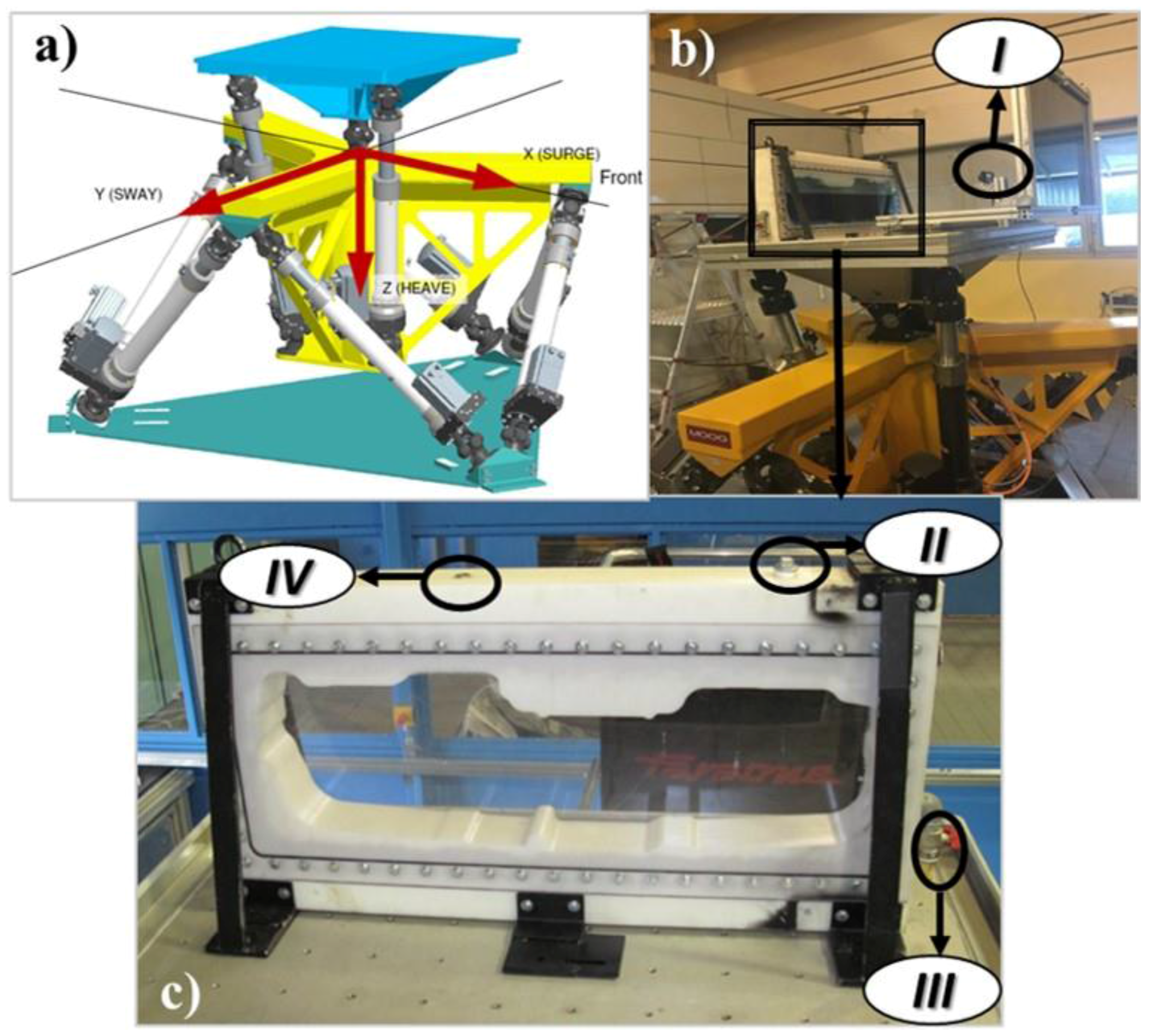
Before describing the developed numerical model to predict the sloshing phenomenon inside a fuel tank, the tank has been tested in collaboration with F.C.A.|Fiat Chrysler Automobiles (Pomigliano d’Arco, Naples, Italy). The bench is shown in Figure 1. It has been designed by Moog Inc. (Elma, NY, USA) flowing the specifications provided by F.C.A. The bench is a hexapod with six independent actuators (with a total stroke of 600 mm) arranged in three triangles. Triangles are connected on the base and the platforms, thus allowing all six DOFs. The top platform is linked to a tilt table with two additional actuators (with a total stroke of 400 mm). This solution allows one to extend the pitch and roll envelope, thus the name of “8-DOF bench” [15].
The hexapod design has been conceived based a small payload flight or driving simulators. There are ball screw types of actuators for both hexapod and tilt table. This solution allows a fast response, smooth run, low noise emission and low maintenance. The bench is equipped with an absolute encoder, to continuously monitor the position of the tank, and with a mechanical brake, integrated in the DC servo motor. The maximum excursion of the fuel tank allowed by the system is more than 400 mm in every direction, reaching peak accelerations of about 1 g (~10 m/s2). Pitch and roll rotation excursions, including the tilt table, reach over 50 deg. With the described test bench, it is possible to reproduce combined sway and surge accelerations of 1 g peak amplitude down to a frequency of about 0.7 Hz. This cuts out much of the low frequency dynamic that is very relevant for automotive applications. The tilt table allows one to simulate lower frequency accelerations using pitch and roll inclinations of the tank assembly. In this way, it is possible to reproduce experimentally the overall effect on fluid motion of very long accelerations, and changes like curves, speeding up and braking.
As clearly shown in Figure 1b, the tank (highlighted in the black rectangle) has been located inside a rigid steel frame, representing installation conditions in the vehicle. The frame is then fixed on the top platform of the tilt table.
A Moog Replication software package (The integrated Test Suite, Moog Inc., Elma, NY, USA) manages the test bench. The software allows to define, view and edit the command signals, to operate and monitor the test, to operate signal identification and matching. The Moog Replication software has been specifically configured for the “8-DOF bench”. The bench, of course, includes many sensors. In fact, there are:
- -
- XsensMTi G-700 ™ (Xsens, Enschede, Netherlands), measuring all six components of acceleration, plus magnetometer and GPS.
- -
- Gyroscopes and tridimensional magnetometers make up the employed inertial platform. Gyroscopes that are also able to record rolling, pitching and yaw.
Even if the bench is able to obtain the rolling, pitching and yaw, in this paper the comparison between experimental and numerical data has been done only for the translation. Equations for the translation follow a harmonic law reported below, where the frequency is of 0.7 Hz and 0.5 Hz:
The research is still in progress therefore the effects on the sloshing due to rotation are currently under investigation. Figure 1 shows the F.C.A. company test bench. In particular, in Figure 1a a 3D drawing of the bench is shown, where the automotive tank under investigation has been located during tests. The tank is clearly shown in the black rectangle in Figure 1b where, with the ellipse at the point (I the high-resolution camera located in front of the tank) has been highlighted. The camera has been rigidly fixed on the tilt table over the platform with an adjustable rod. Of course, it is necessary to fix the digital camera in the way to film any test performed at the bench and at the same time to maintain the position of the tank. The camera, as shown in Figure 1c, is interposed between the tank and an opaque black panel in order to reduce reflection of the Plexiglas panel of the tank and, consequently, improve the video quality. The camera used has a resolution of 1280 × 720 pixels and shoots 25 frames per second. In Figure 1c a zoomed view of the tank is shown. Point II in figure is the fill sensor, III is the air vent while IV is the exhaust valve of the tank.
Dynamic tests have been performed on a tank properly designed for the study made by high-density polyethylene and Plexiglas (see Figure 1c) and it was fixed to the Moog test bench by means of two L-shaped steel profiles to ensure a high rigidity of the system during any test condition. Starting from the central section of a multilayer plastic tank of a F.C.A. commercial vehicle the tank polyethylene shape has been drawn. The designed and tested tank has exactly the same section of a production automotive tank thus two dimensions, width and height, are the same. The third dimension (depth) is lower (of 100 mm, about ¼ or ⅕ lower than the original tank). The depth has been modified introducing two faces in Plexiglas to capture the fluid oscillations during the tests. Therefore, the prototyped tank is 870 mm in length, 265 mm in height and 100 mm in depth and front and back transparent plates have 5 mm of thickness. It has been designed not only to observe the sloshing phenomenon but also to guarantee resistance, rigidity and waterproofness. The tank, during the test, is completely closed; therefore, no gas or liquid can enter or exit from the system.
As already mentioned, the working fluid is simply water colored by a dark blue food colorant. The choice of the water as a working fluid has been done to easily monitor the sloshing phenomenon. The choice is also strategic because of the safety, the simplicity of disposal and the unlimited availability at no cost. Therefore, as a multiphase application, the properties of both phases are listed in Table 1.
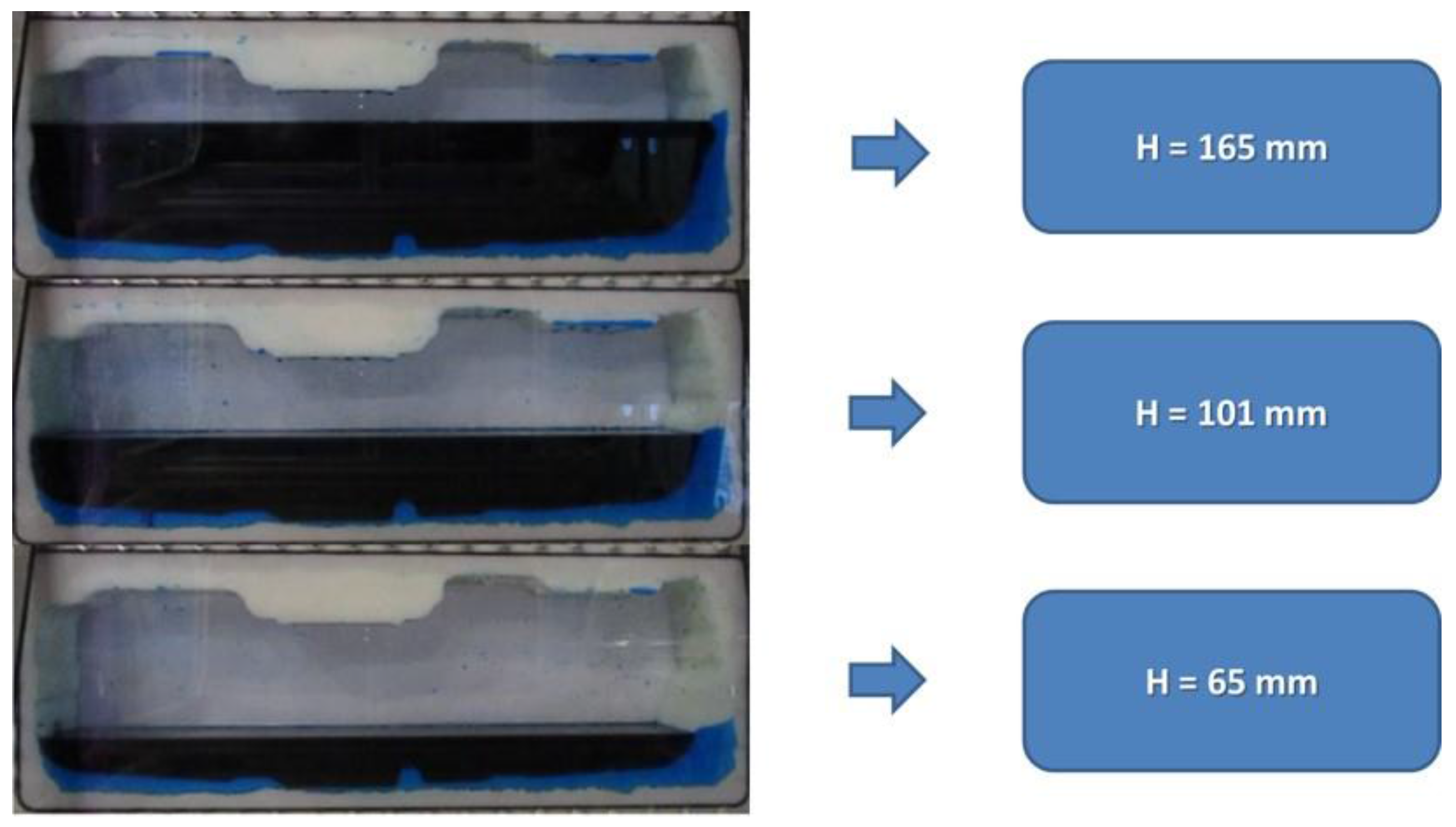
Tests have been done for three different free surface levels H. The tank has been filled at:
- H = 165 mm;
- H = 101 mm;
- H = 65 mm.
In Figure 2 the three levels are shown. Numerical simulations have been done for each fluid level in the tank and results have been compared with tests with a high agreement.
In order to compare tests with the numerical results images post-process is necessary. All the pictures captured by the camera highlighted in Figure 1b have been analyzed using Matlab®. The post-processing phase has been done in order to obtain clear images usable to obtain important information like the center of gravity and the free surface.
3. Images Post-Processing
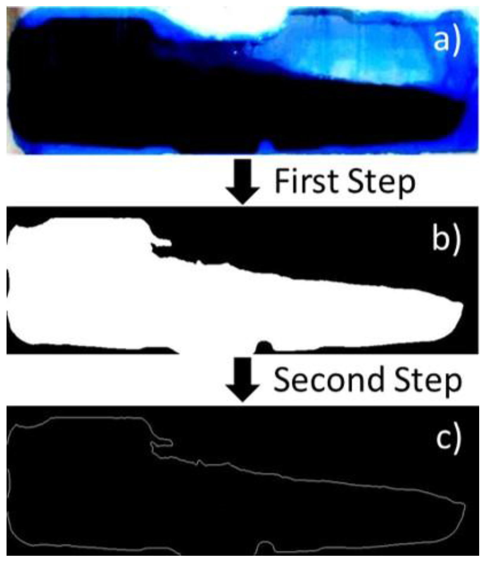
Experimental images described in the Section 2, as said, need to be post-processed to be comparable with results of the three-dimensional CFD model that will be described successively. For this reason, both experimental and numerical data have been compared after a picture enhancement treatment performed with Matlab®. Figure 3, as example, shows the experimental image before and after the post-process. In particular, Figure 3a is the image captured by the camera with enhanced contrast only while Figure 3b is the image after post-processing. The images after the post-processing phase consists of a sequence of steps. The initial image (i.e., Figure 3a) is uploaded in Matlab® where is cleansed of all parts not needed for analysis, as example the blue food coloring deposited on the first Plexiglas face visible in Figure 3a. Then the picture is turned into a black and white image as shown in Figure 3b. In particular, the liquid becomes white while the air is black. Then picture in Figure 3b is further post-processed in order to identifying the exact border between air and water for each condition. The final post-processed image is shown in Figure 3c.
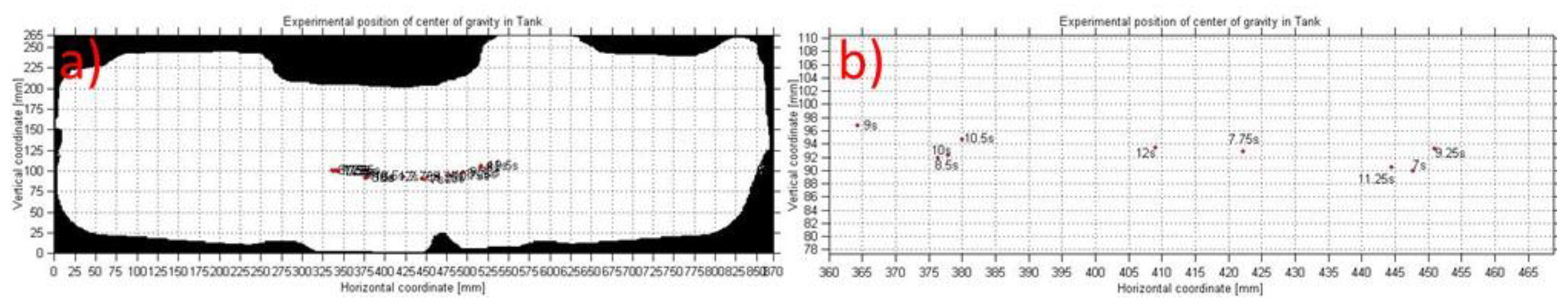
The last step of the post-processing process in Matlab® is presented in Figure 4, where for each time instant the center of gravity is correctly obtained [17]. Therefore, this evaluation has been done for each time instant in the range [7 ÷ 12] s with a time step of 0.25 s. Figure 4, in fact, shows the position of the center of gravity during tests step by step. In Section 5 of this paper, the experimental data and numerical results have been compared to estimate the accuracy of the simulation model on the free surfaces and the centers of gravity.
4. Numerical Model Description
From the numerical point of view, the adopted methodology consists of a three-dimensional CDF approach developed using the commercial code PumpLinx® (V4.6.3, Simerics Inc., Bellevue, WA, USA) [18]. The numerical model has been built up including new capabilities to correctly predict the flow behavior of two immiscible fluids, separated by a well-defined interface. Thus, the model consists of two immiscible fluids in movement separated by an interface. In particular, in this section, all equations governing the phenomena are presented separately.
The model mathematically describes the fluid flow solving the equation of conservation of mass and momentum. Furthermore, to describe correctly the fluid sloshing inside the tank, additional properties, such as viscosity, surface tension and compressibility, have been implemented as input for the simulations.
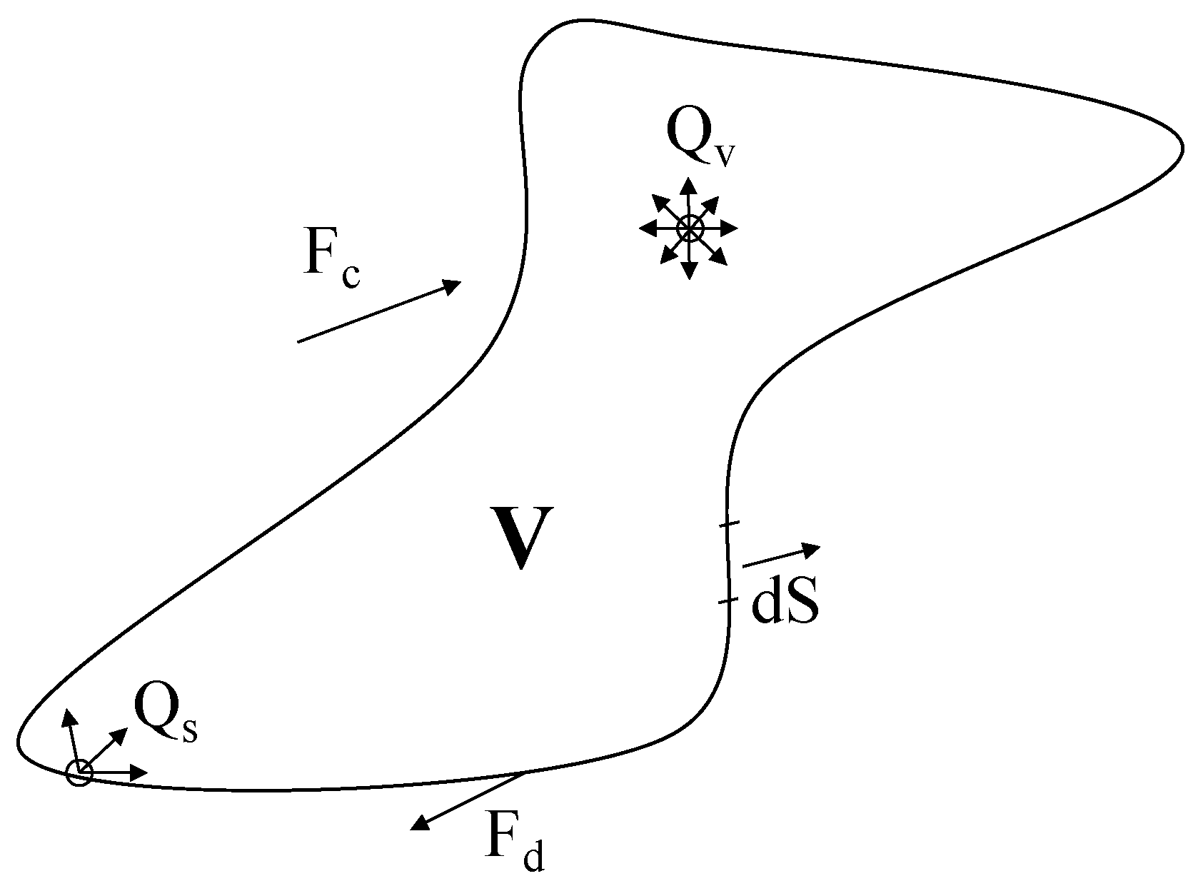
Considering a flow quantity and a control volume reported in Figure 5 [15,17,18,19], the Gauss’s theorem can be applied as reported into the equation:
where indicates the time, is the convective flux over the boundary due to the motion of the fluid, is the fluid velocity, is the flux over the boundary conditions due to diffusion, is the volume of the control volume, is the internal source, the source at the boundary. In the analyzed case the and the (the internal source and the source at the boundary) are the gravity and the displacement law variation (function of the frequency) acting on the fluid volume of the tank.
If the flow quantity is the mass, the transport equation can be defined as in (3) assuming no sources such as chemical reactions or phase changes in the system. Equation (3) is also known as the continuity condition. It states that, for the incompressible case, the mass of a fluid in a closed domain can only be changed by flow across the boundaries:
Before to describe the built model, it is important to deeply describe the methodology adopted presenting the equations solved during simulation. Particular attention must be reserved to the definition of the model for the turbulence. In this application, good results have been achieved using the Re-Normalization Group (RNG) k − ε model for the turbulence. In fact, for the specific problem it has proven to be really accurate. The standard k − ε model, used for the simulations presented in this paper, follows the two equations reported below [20,21,22,23,24,25,26,27]:
with = 1.42, = 1.68, = 1, = 1.3, is the fluid velocity and is surface motion velocity while and are the turbulent kinetic energy and the turbulent kinetic energy dissipation rate Prandtl numbers. As said in Section 2 of the paper, the designed tank has been tested for three different liquid levels. The container is filled by water and air therefore simulations need to solve a multiphase flow. This type of flows is better solved with explicit numerical schemes, especially if an accurate prediction of the free surface is required. To achieve a stable solution, these schemes require the Courant-Friedrichs-Lewy condition to be satisfied. This condition is defined by Equation (6):
The magnitude is the Courant Number and it represents the distance that the interface between two components would travel, across a mesh cell, during one time-step. The Courant Number controls the sub time-steps size in the calculation of the transport of the components for the multiphase module. In the code PumpLinx®, the Courant Number is set to a default value of 0.34, with a lower number providing more accuracy but, on the other hand, longer simulation time.
The calculation of a sub time-step, Δtsub, is performed only for the cells in the domain that have a mixture of components. Then the smallest of those calculations is used as the sub time-step, Δtsub, for updating the transport of the components.
As mentioned above, an explicit method preserves the shape of the interface between components and it is more accurate than the implicit one. A Blending Factor (BF) is used in conjunction with the higher order interpolation schemes (e.g., Central and 2nd Order Upwind) to help stabilizing the convergence by including the 1st order Upwind scheme using the formula reported below [17,25]:
Higher values of the Blending Factor make the solution more stable, but potentially at the expense of accuracy. Therefore, a typical value falls in the range from [0 ÷ 0.5]. In this study, it is zero.
First of all, before running the simulation, the gravity force (in this case, the direction is along the z-axis) has been included in the model. In thermodynamics, surface tension is dealt with on a macroscopic level based on the statistical behavior of interfaces [3]. Sabersky and Acosta [20] noticed that it is better to consider the microscopic level to understand the mechanism of this phenomenon. In fact, many other molecules surround a liquid molecule and away from the interface.
The surface tension coefficient σ is defined by Yuan [21] and by Massey [22]. It is the amount of work necessary to create a unit area of free surface. It always exists for any pair of fluids, and its magnitude is determined by the nature of the fluids. For immiscible fluids, the value is always positive and for miscible fluids such as water and alcohol, it is negative [9].
An important aspect of surface tension is that it creates a pressure jump Δp across a curved surface. The following equation correlates the pressure jump across a curvature surface with the surface tensor:
where and are the principal radii of curvature of the surface, is the mean curvature, is the surface tension coefficient and is the pressure (the larger pressure is on the concave side of the curved surface).
In order to achieve the final goal of the study, some assumptions have been fixed. First of all, the flow inside the tank is incompressible, Newtonian and homogenous with a density and viscosity μ constant. At last, the temperature dependence has been not considered. Furthermore, the is considered equal to the tank velocity on the tank walls; therefore, there are non-slip conditions on the walls. As said, the analysis has been done considering two immiscible fluids subject to external forces. The flow of immiscible fluids can be classified into three classes; these classes have been already described in the introduction section. The first class concerns the sloshing in this case where the two phases remain separated with a single well-defined interface with a motion with low frequency and amplitude. Thus, this study falls in the first one because oscillations are gently with a low amplitude and frequency. The same modeling approach can be used also in the other two classes of sloshing already defined in the introduction (classes two and three).
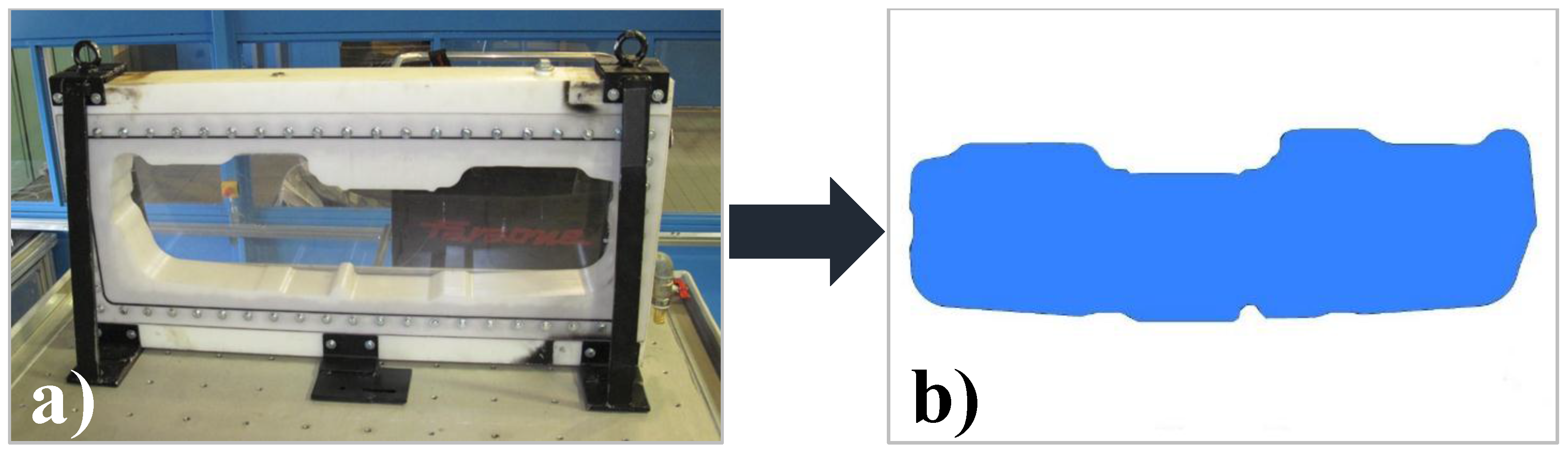
The experimental setup has been replied using a three-dimensional CFD numerical approach [15,21,22,23,24,25,26]. Therefore, starting from the real CAD geometry of the prototype tank, the fluid volume has been extracted and then meshed. The fluid volume of the tank is shown in Figure 6b. This volume has been extracted from the real fuel tank in Figure 6a.
As a study of two immiscible fluids, before importing the geometry in the simulation code for the grid generation, it is important to define in advance the initial (static) free surface for each simulation. The liquid level has been already indicated with the letter H. Experimental tests have been done for three H levels:
- -
- H = 65 mm;
- -
- H = 101 mm;
- -
- H = 165 mm.
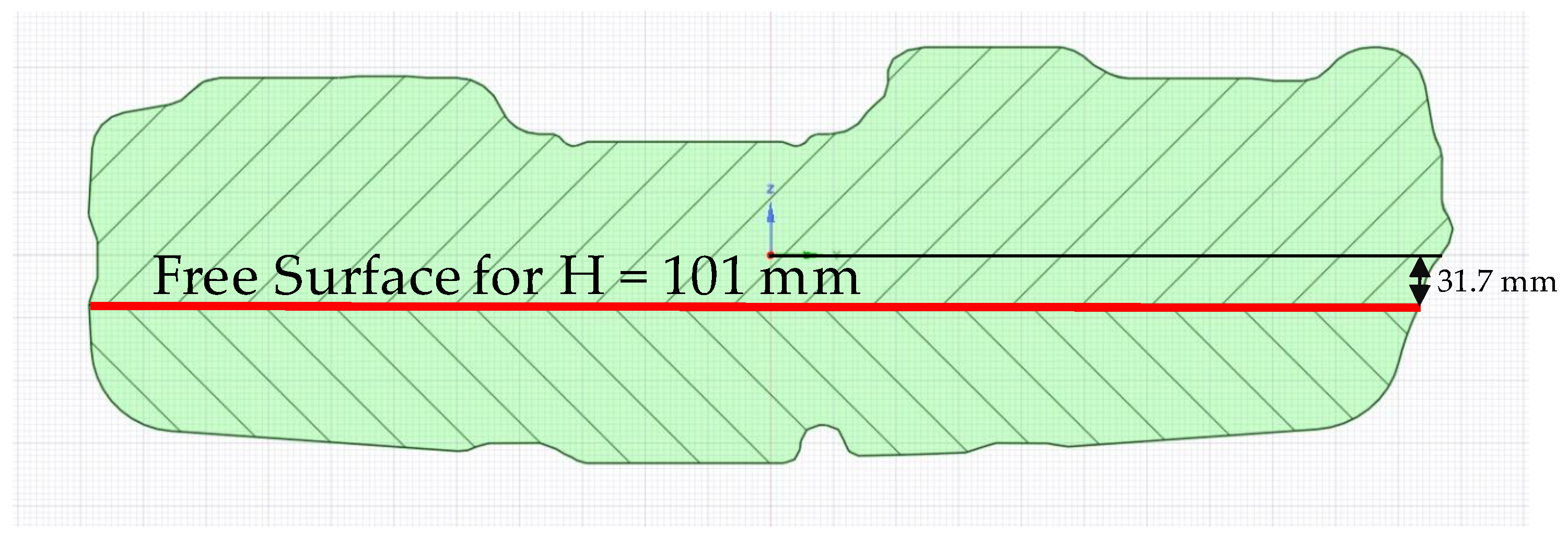
In Figure 7 the free surface in the tank drawing at H = 101 mm is presented. Each dimension has been taken with respect to the coordinate (0, 0, 0), center of the drawing. The bold red line in Figure 7 represents the considered free surface of one of the three analyzed cases.
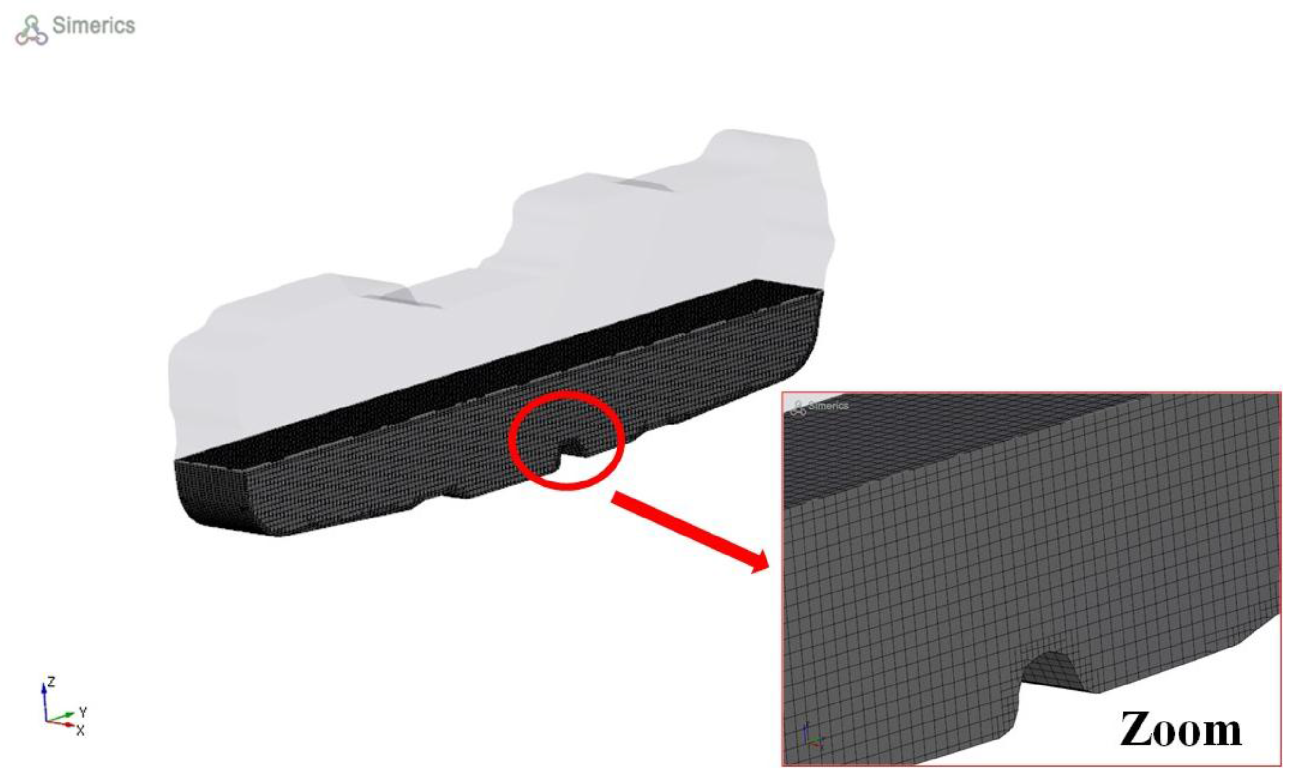
The extracted fluid volume in Figure 6b has been meshed using a body-fitted binary tree approach. This grid type is accurate and efficient because the parent-child tree architecture allows for an expandable data structure with reduced memory storage. In this architecture, the binary refinement is optimal for transitioning between different length scales and resolutions within the model. The majority of cells are cubes, which is the optimum cell type in terms of orthogonallity, aspect ratio, and skewness thereby reducing the influence of numerical errors and improving speed and accuracy. It is important to underline that since the grid is created from a volume, it can tolerate inaccurate CAD surfaces with small gaps and overlaps.
The entire grid of the tank fluid volume is shown in the Figure 8 with also a zoom view of the grid in a particular area around edges. With the described grid generation approach, it has been demonstrated [15] that it is possible to reach good accuracy and low computational time also by increasing the grid density in the boundary layer and on the surface. However, in case of multiphase simulation, it is better to have a mesh as uniform as possible. The zoomed view in Figure 8 shows that in this particular application the generated mesh almost is uniform, especially around edges. To better simulate the sloshing phenomenon, the grid has been subdivided and cut in the regions of high curvature and small details.
Due to the complex analysis it has been selected the automatic refinement algorithm of PumpLinx® for the mesh generation. With this approach, it is possible to assign a maximum and a minimum cells size (and, of course, the cell size at the walls) and the mesh generator automatically adapts the refinement strategy and the levels of refinement as a function of the prescribed values and the geometry provided. This is a proprietary methodology developed by Simerics Inc. (Simerics Inc., Bellevue, WA, USA), the code developer.
A maximum cell size parameter of 3 mm has been chosen, whereas the minimum cell size parameter has been fixed at 0.5 mm. The maximum cell size is a parameter used to build the grid which controls the size of the cells while the minimum cell size is a parameter used to limit minimum dimension of cells. This means that, no cell in the volume can have a cell side smaller than the minimum cell size. At last, the cell size on surfaces also needs to be fixed. This parameter is used to control the size of the cells for all surfaces of a mesh volume.
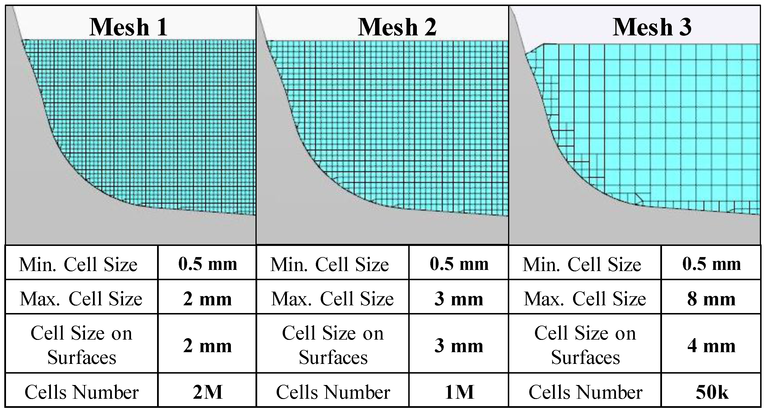
As a dynamic phenomenon, simulations are transient and have been run on a multi-core Windows® 64-bit PC (CPU with two Intel(R) Xeon(R) E5-2640 v2 processors operating at @2.00 GHz, equipped with 192 Gb RAM). Before showing the numerical results, it is important to underline that, as normally done, a mesh sensitivity analysis has been performed.
Figure 9 shows three of the generated meshes. The first grid called “Mesh 1” consists of 2 million cells. The maximum cell size and the cell size on surfaces have been set to 2 mm while the minimum cell size is of 0.5 mm. The grid called “Mesh 2” consists of 1 million cells with a maximum cell size and the cell size on surfaces set to 3 mm and with the same value of the “Mesh 1” for the minimum cell size. The grid called “Mesh 3” has only 50.000 cells. Also in this case the minimum cell size is of 0.5 mm while the other two parameters are higher than in other cases.
Simulations have been run for the three meshes with the same boundary conditions and results with 1 million and 2 million cells have demonstrated the same level of agreement with the experimental data. However, the model with 2 M cells has higher computational time than the one with 1 M cells. At the same way, even if the computational time of the mesh with only 50.000 cells is lower than for others, results are too far from the experimental data. For these reasons, in this study the mesh size of one million cells has been employed; it shows excellent accuracy and low computational time.
Having built the mesh of the model, it is important, before running simulations, to set all the input parameters. In this case, the fluid level is one of them. It can be set writing the Equations (11) and (12), reported in the following paragraphs, in the expression editor panel of the code. It automatically splits the fluid volume of the tank, in Figure 7, into two phase ao and wo where ao is the air and wo is the water. Equations (11) and (12), therefore, define the percentage of filling of the tank. In this research, three levels of filling the tank have been studies (called Test 1, 2 and 3) better described in the next section (Section 5). The free surface of the water, for each filling level, evolves during simulation as function of the time, as done during the tests. Both, tests and simulations, last 12 s. In particular, the air level is defined as in the Equation (9) instead the water level in the Equation (10):
Equations (9) and (10) are referred to the free surface level of 101 mm already shown in Figure 7. There is no special mesh treatment at the interface between the air and the liquid. The mesh is uniform across the flow field because the liquid interfaces in this simulation can potentially reach everywhere in the domain and change very quickly through time. A surface tension of 0.0073 N/m has been applied on the water. As known, the surface tension depends on the combined properties of the fluids on either side of the interface, but for the current release, the surface tension is limited to associating it to only one component, even for multiple fluids.
As done during tests, an assigned displacement along the direction y for the entire tank has been assigned as input for the model. The displacement law variation has been already shown in the paper Section 2 (Equation (1)). The displacement law variation is, therefore, function of the frequency (0.5 Hz and 0.7 Hz) and time. In order to replay the experimental data, simulations have been run for 17 s with 340 steps all saved for comparing numerical results with tests in the validation phase.
5. Results and Model Validation
Simulations have been run for the three tested water levels (65 mm, 101 mm and 165 mm) and at both values of frequency, 0.5 Hz and 0.7 Hz, in order to replicate experiments done on the F.C.A. test bench. In this section tests and numerical results are presented and compared. Results comparison has been done by means of the picture visualization for each instant in the range [7 ÷ 12] s with a time step of 0.25 s and by means of the trends of both center of gravity and free surface level in the same time interval. This section has been split into three subsections for the tested water levels.
Tests therefore will be called:
- (1)
- “Test 1” for a water level H of 65 mm,
- (2)
- “Test 2” for a water level H of 101 mm,
- (3)
- “Test 3” fora water level H of 165 mm.
All the analyzed tests include also the comparison between data, experimental and numerical, for the two frequencies.
5.1. Test 1
Before analyzing results, it is important to underline the input provided to the code for the simulation. Inputs are listed below:
- -
- A water level of 65 mm;
- -
- A frequency of 0.5 Hz and 0.7 Hz;
- -
- An amplitude of the oscillations of 0.0811 m.
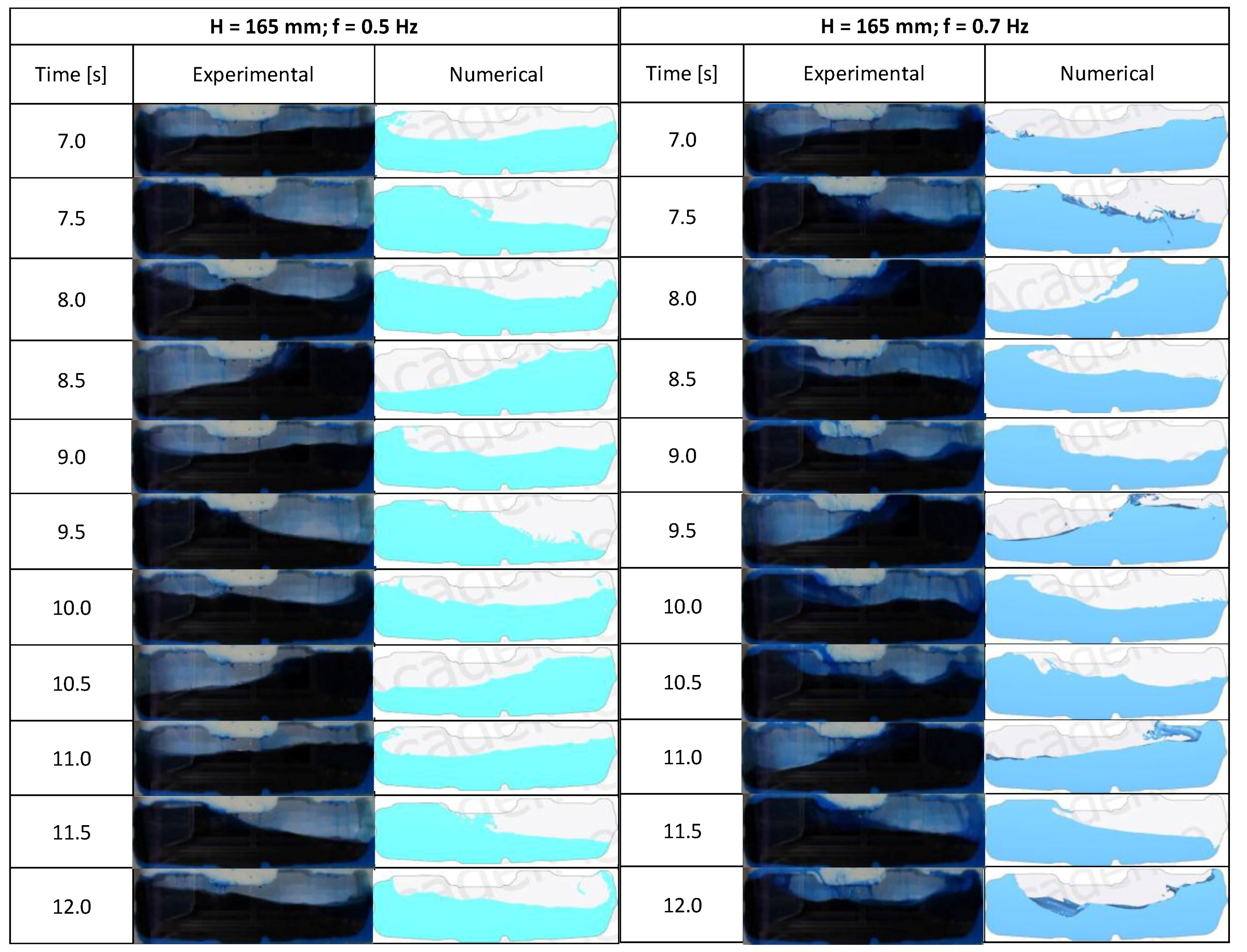
Using the developed data post-processing application and already described in Section 3, the numerical results have been processed to be compared with tests. The image post-treatment, as said, consists of several operational steps. Each picture given by the model is uploaded in Matlab® where it is cleansed of parts not requested for analysis. The comparison between numerical and experimental data is presented in Figure 10. Images in Figure 10 are referred to a time interval [7 ÷ 12] s with a time step of 0.25 s for two frequency values.
In Figure 10 it is possible to observe that the numerical model is capable of predicting sloshing of the Test 1 with visibly good accuracy. However, the comparison was also done by evaluating the center of gravity and the free surface of the fluid in the abovementioned working conditions. To perform this analysis the images in Figure 10 have been post-processed and turned into black and white ones, as already shown in Figure 3b. In this way, the center of gravity can be estimated. Then the black and white pictures have been further treated to isolate the free surface profile, as already shown in Figure 3c. Images in Figure 10 have been post-elaborated with Matlab® identifying the center of gravity at both frequency values in the time interval [7 ÷ 12] s with a time step of 0.25 s. For the Test 1, the comparison on the center of gravity and the free surfaces between numerical and experimental data are reported in Figure 11 and Figure 12.
The comparison has been done along the horizontal and the vertical axis. Both the horizontal and the vertical displacements in millimeters of the center of gravity are reported as a function of the time. The black line is always related to the numerical results while the red one to the tests. The trends of the numerical and the experimental data displacements in Figure 11 are almost the same for both frequencies. The gap between the data of each graph has been evaluated showing that the error is always close to zero as confirmation of the model accuracy. The maximum error percentage and the standard deviation between numerical and experimental data have been reported in Table 2, for both frequency values. In the table, there is also reported the simulation time for each run.
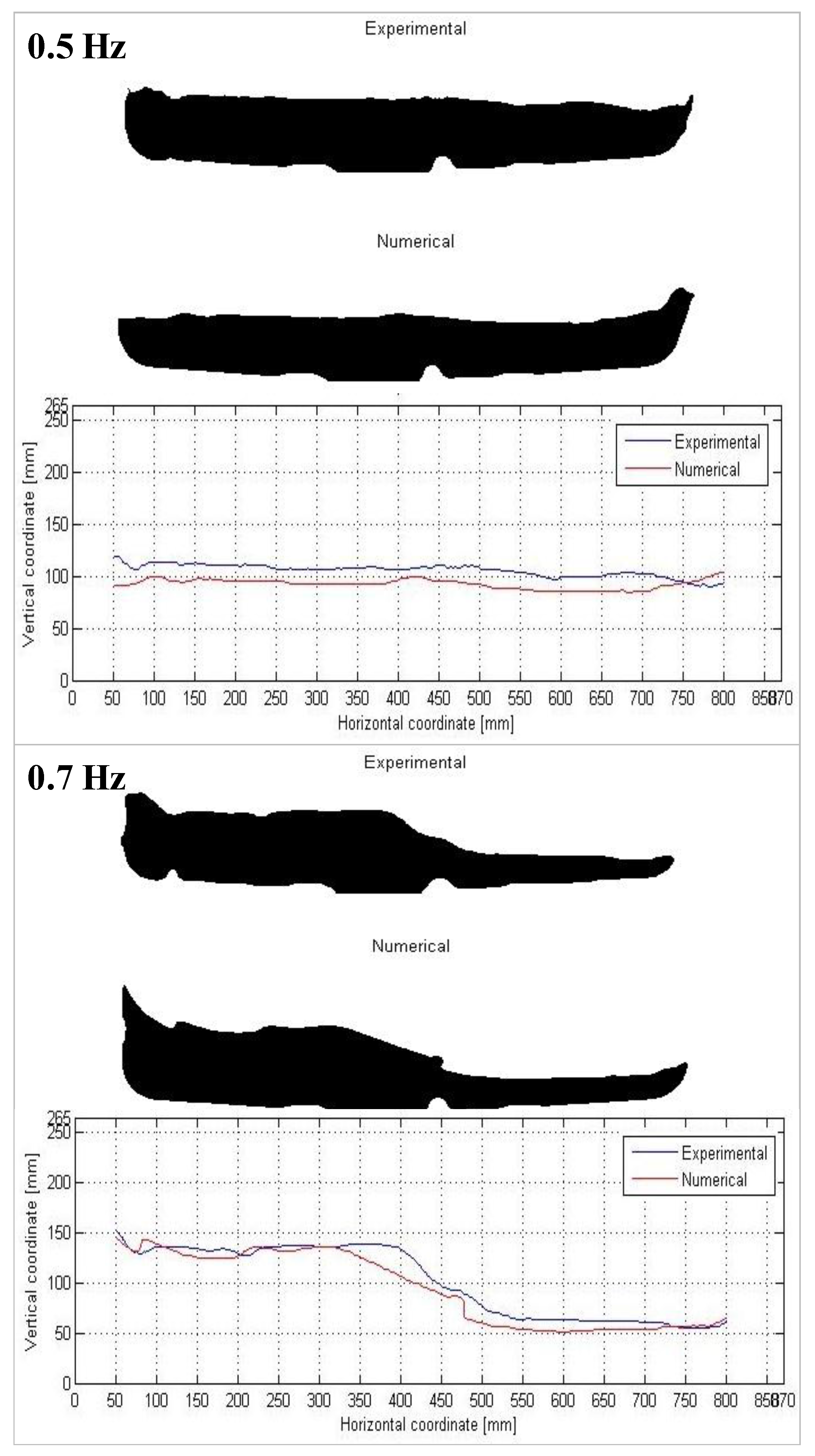
The study performed on the center of gravity has been carried out also on the evaluation of the free surface profile in the same time interval [7 ÷ 12] s with step of 0.25 s. As shown in Figure 3c) of Section 3, using the developed code in Matlab®, free surfaces can be isolated and post-elaborated.
Therefore, starting from images in black and white the free surface for a specific time instant can be diagrammed (Figure 12). These graphs, in fact, report the free surfaces comparison between numerical (red line) and experimental data (black line). Gaps between data have been evaluated per each time instant and for both frequency showing that the numerical model is able to predict with high accuracy the free surface of the liquid, step by step. In Table 3, as already done for the center of gravity in Table 2, the standard deviation and the error percentage of the free surfaces are reported in the time interval [7 ÷ 12] s with a time step of 0.25 s. The average error percentage is very low; in fact, it is only of 3.9. The average error percentage is calculated, with steps of 0.25 s, from the standard deviation compared to the height of the tank since it has been evaluated on the vertical for each abscissa.
5.2. Test 2
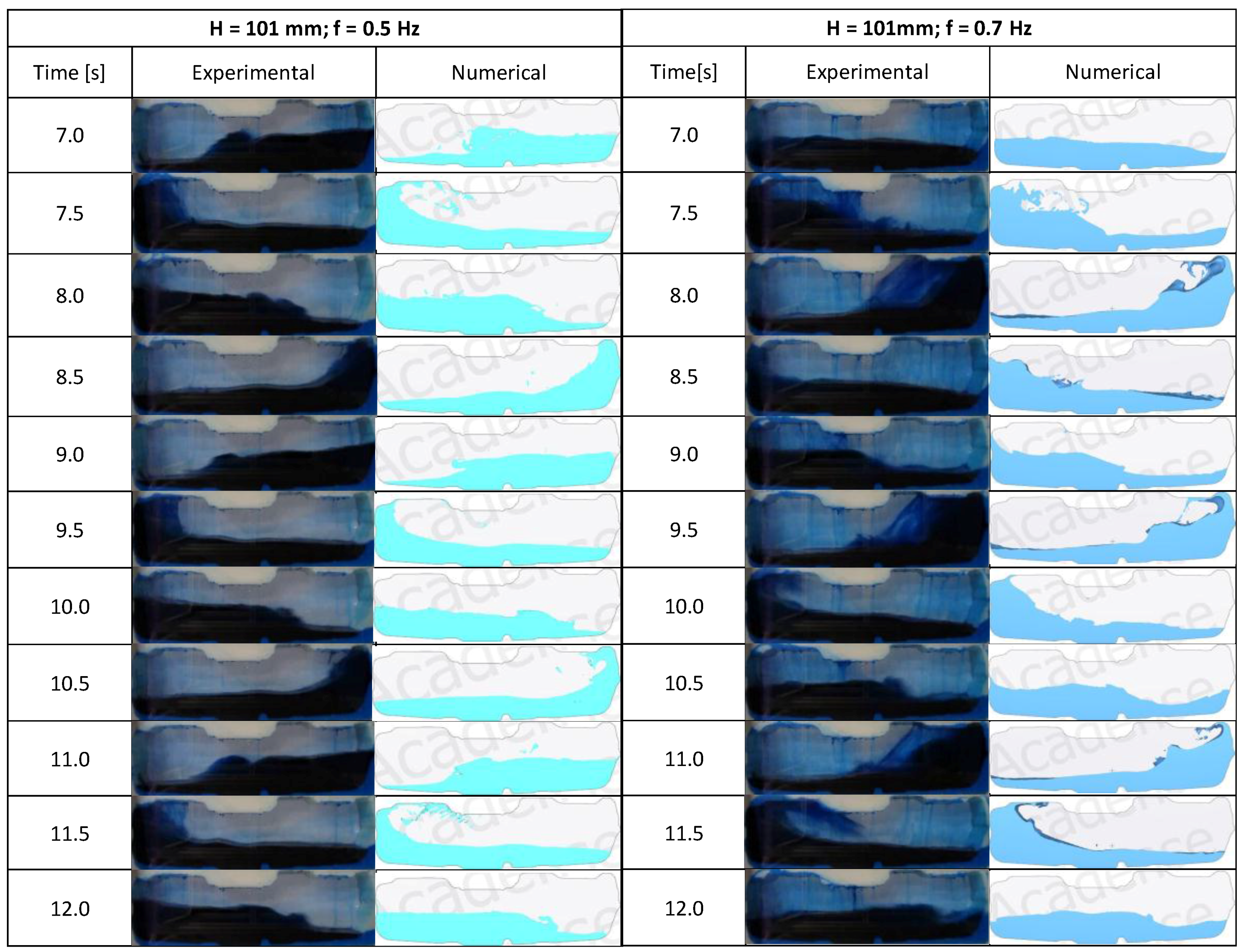
“Test 2” corresponds to the study with a liquid level of 101 mm. As already done for Test 1, before showing the simulation results, it is important to remember the working conditions that are listed below:
- -
- A water level of 101 mm;
- -
- A frequency of 0.5 Hz and 0.7 Hz;
- -
- An amplitude of the oscillations of 0.0781 m.
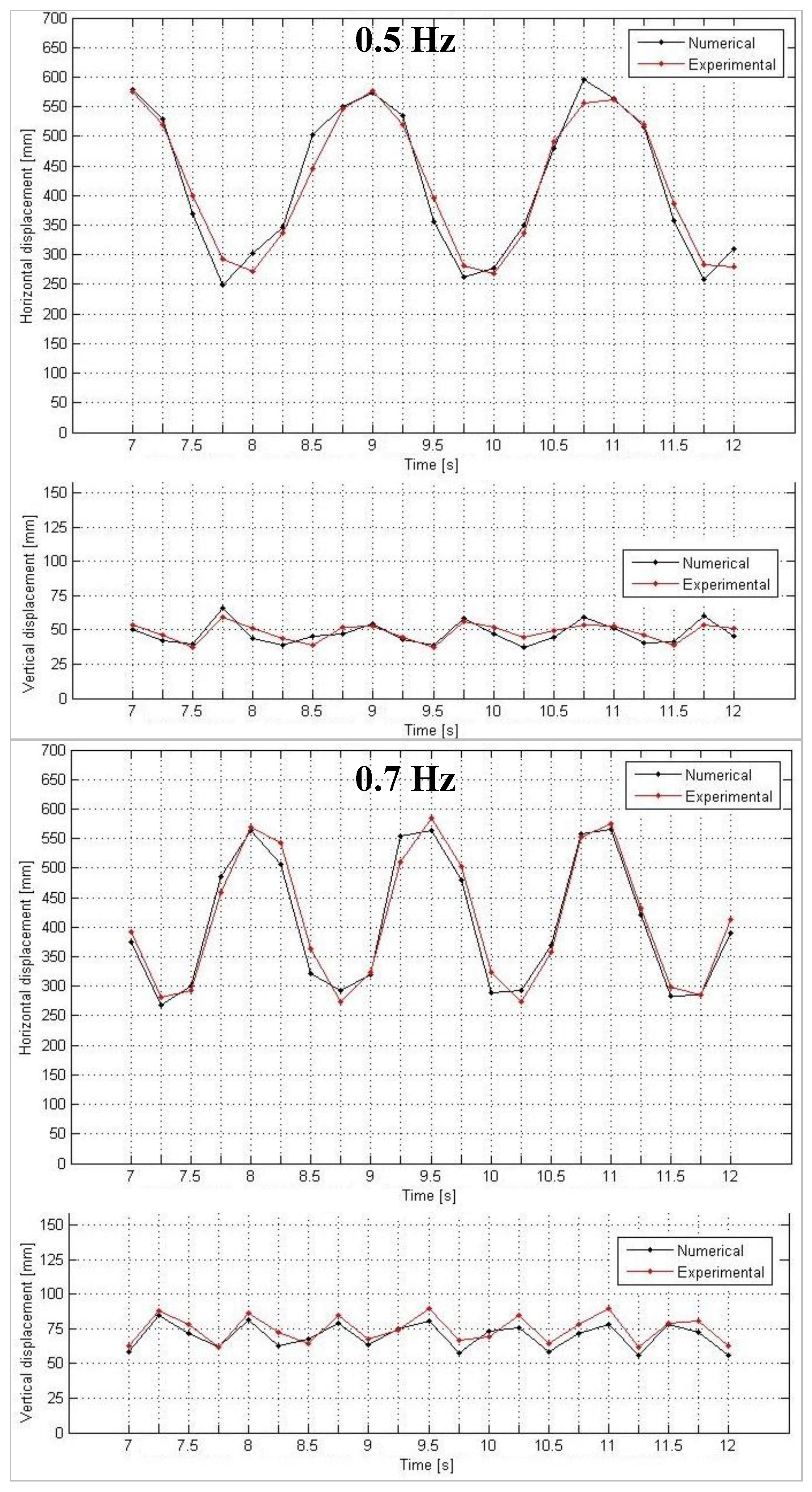
In Figure 13, the simulation results are compared to the experimental data. Analysis has been performed in the same time interval [7 ÷ 12] s and with the same time step of 0.25 s.
Using the already described post-processing methodology, the images in Figure 14 have been analyzed comparing the center of gravity and the delta along the horizontal and vertical axis. The analysis shows, also in this case, a good accuracy of the numerical model.
The error percentage and both standard deviations (vertical and horizontal) of the center of gravity are reported in Table 4. In this case, the comparison shows a maximum error percentage of 2.5%. In Table 4 there are also reported the simulation time for both frequency values which are always below 3 h.
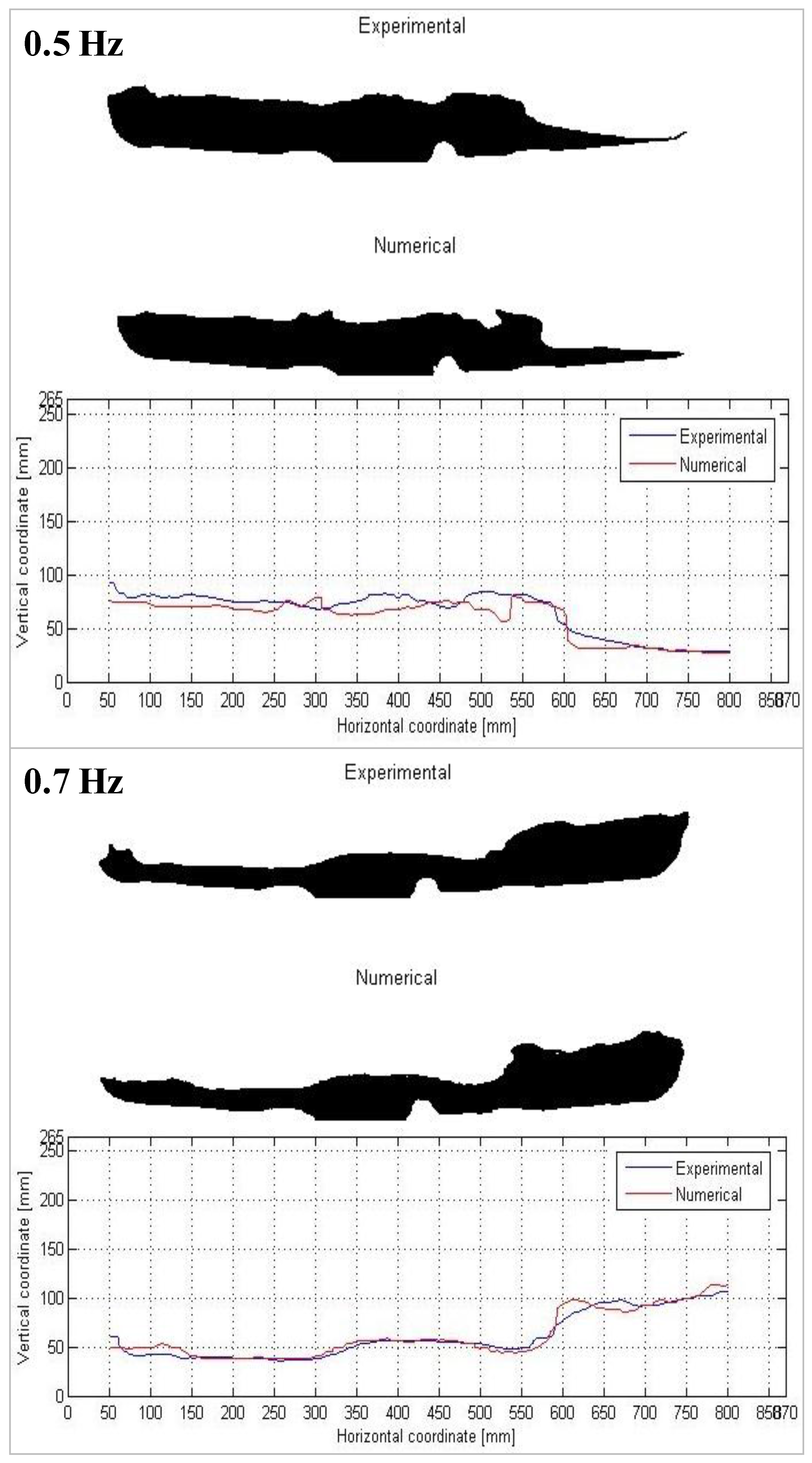
Free surfaces have been analyzed and the comparisons between numerical and experimental data are shown in Figure 15. Also in this case the free surfaces have been post-elaborated in order to quantify the error percentage and the standard deviation of the simulation results with respect to tests. Table 5 presents, in fact, the standard deviation and the error percentage of the free surfaces for the Test 2, in the time interval [7 ÷ 12] s with a time step of 0.25 s. The maximum error percentage in this case is 5.9%.
The mean deviation standard in Table 5 for a frequency of 0.5 Hz is 12.0 mm with a final error percentage of 4.2% while for the frequency of 0.7 Hz the deviation standard is 16.2 mm with a final error percentage of 5.9%. As said, the average error percentage is calculated, with steps of 0.25 s, from the standard deviation compared to the height of the tank.
5.3. Test 3
The last analysis concerns the case called “Test 3” where the water level is equal to 165 mm. Model inputs are:
- -
- A water level of 165 mm;
- -
- A frequency of 0.5 Hz and 0.7 Hz;
- -
- An amplitude of the oscillations of 0.0811 m.
In Figure 16, the simulation results and experimental data are compared. The analysis has been performed, also in this case, in the time interval [7 ÷ 12] s and with the same step of 0.25 s.
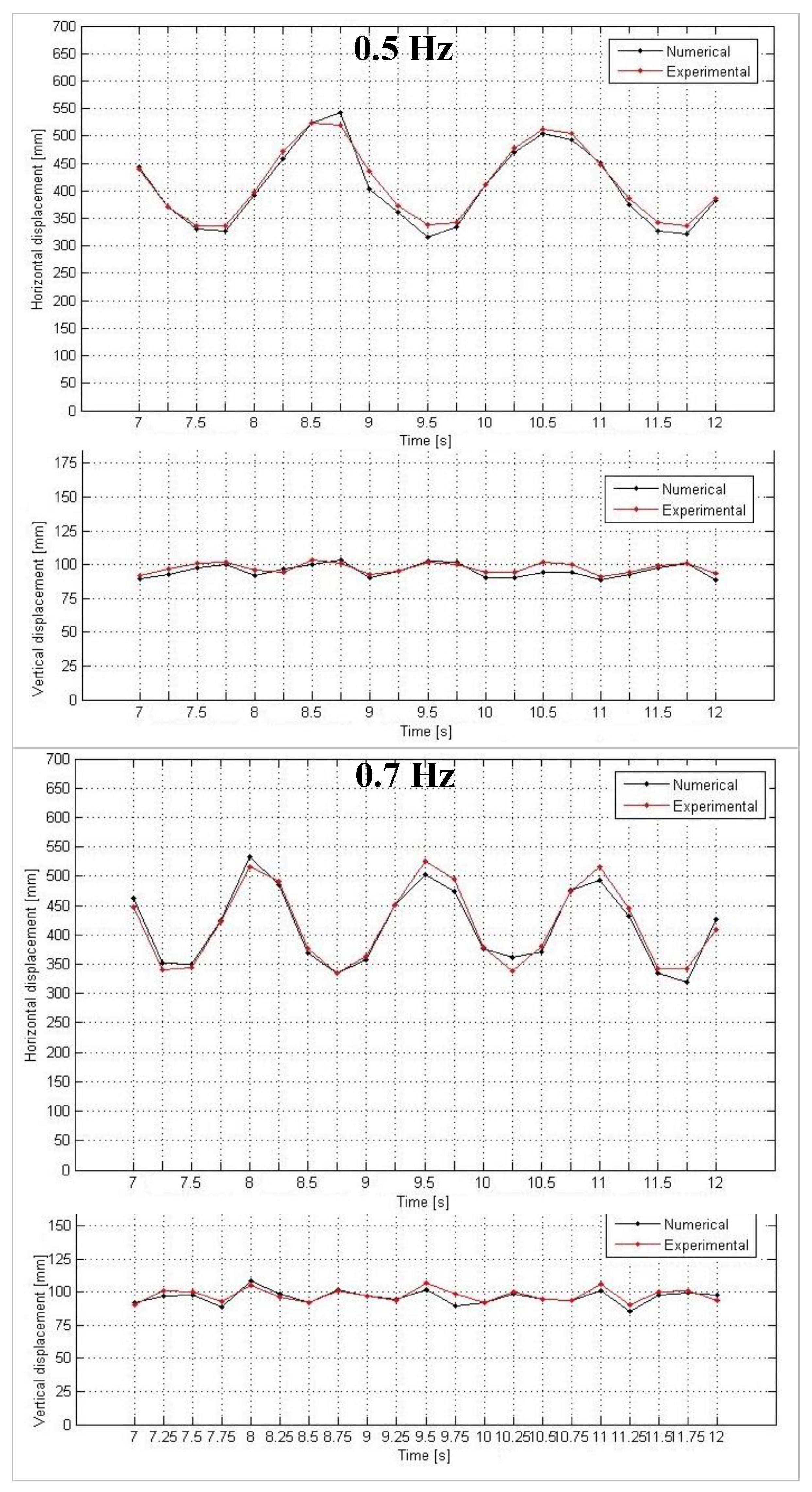
All the pictures in Figure 16 have been analyzed comparing the center of gravity and, of course, the horizontal and vertical displacements. The analysis shows, also in this case, a good accuracy of the prediction model.
The error percentage and both standard deviations (vertical and horizontal) of the center of gravity are reported in Table 6. In this case, the comparison shows a maximum error percentage equal to 1.6%. In Table 6 the simulation time for both frequency values are also reported, which are always below 4 h and half. In this case, for a frequency of 0.5 Hz the mean horizontal deviation standard is equal to 10.9 mm, while the vertical deviation standard is 2.76 mm with a final error percentage equal to 1.26% and 1.04% respectively. For a frequency of 0.7 Hz the mean horizontal deviation standard is equal to 14.1 mm while the vertical deviation standard is 3.34 mm with a final error percentage of 1.62% and 1.26% respectively.
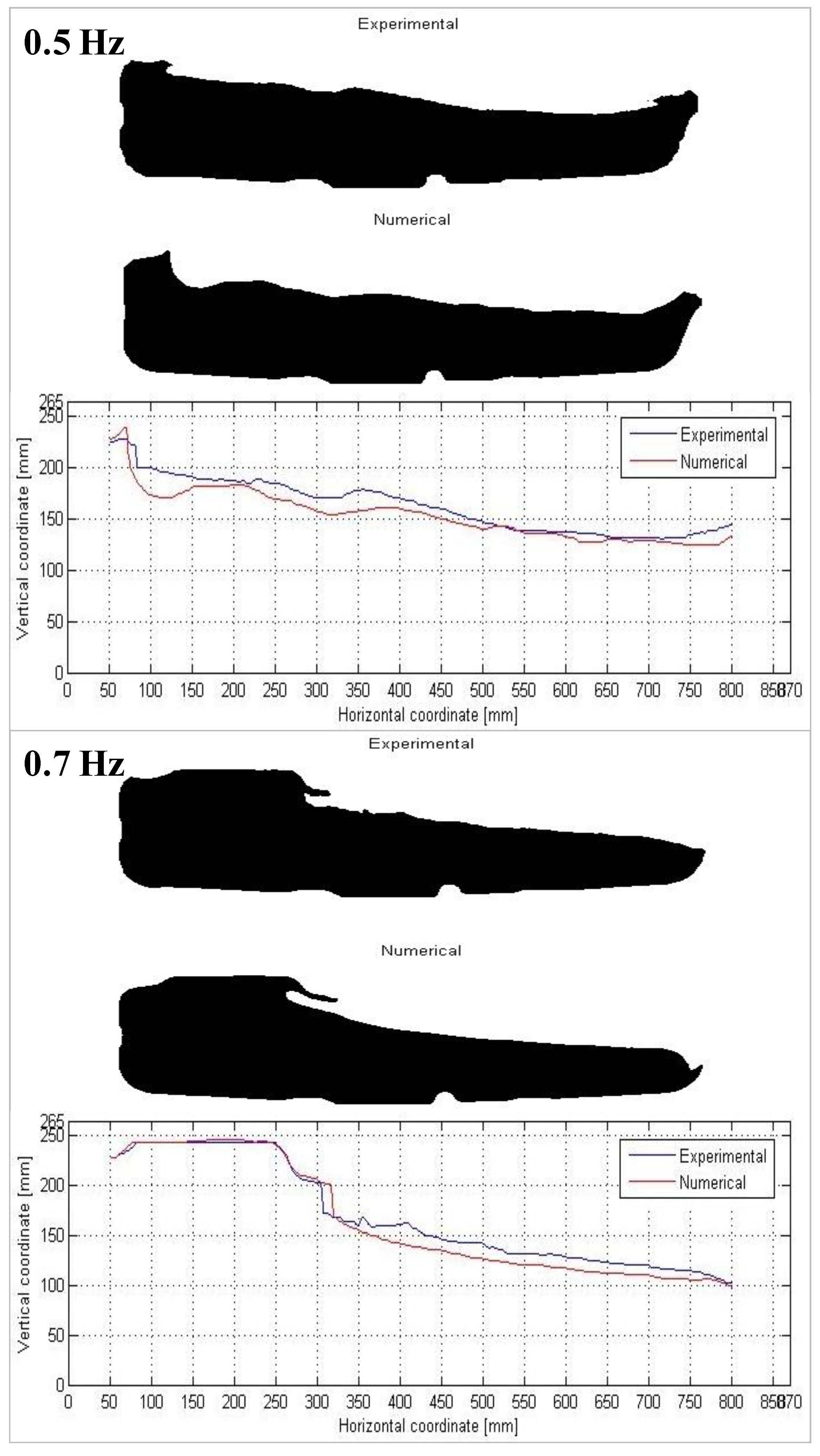
At the same way, the post-process phase has been done on the free surface of the fluid and the results are shown in Figure 17. Also in this case, the free surfaces and the comparison between numerical and experimental data have been analyzed.
Finally, the results in term of standard deviation and the error percentage of the free surfaces for the Test 3 are shown in Figure 18 and in Table 7, always in the time interval [7 ÷ 12] s with step of 0.25 s. The maximum error percentage in this case is of 5.6%.
As said, the average error percentage is calculated, with steps of 0.25 s, from the standard deviation compared to the height of the tank.
Looking at table, the mean deviation standard for a frequency of 0.5 Hz is equal to 15.3 mm with a final error percentage of 5.6% while for the frequency of 0.7 Hz the deviation standard is equal to 16.5 mm with a final error percentage of 5.6%.
6. Conclusions
A numerical and experimental study on the sloshing phenomenon inside a vehicle fuel tank has been described in this paper. The research was undertaken to find a methodology able to correctly predict the real phenomenon. For this reason, an experimental investigation was carried out to validate a three-dimensional CFD model. Tests were performed on a dedicated test bench designed by Moog Inc follwiug the specifications provided by Fiat Chrysler Automobiles (F.C.A.). It is a hexapod with six actuators which are independent. The actuators are located in three triangles designed to connect the top to the base platform, thus allowing all six DOFs. The experimentation has been done for three filling levels of the container.
The entire fuel tank has also been studied with a three-dimensional modelling technique. The CFD model was built up using a CFD commercial code and integrating a multiphase tool in order to correctly reproduce the real free surface. Numerical and experimental data have been compared after post-processing carried out using Matlab®. The comparison showed a maximum error percentage between data of maximum 5.6% both on the estimation of the free surfaces and on the centers of gravity of the fluid. The numerical model, therefore, predicts correctly the interfacial structure that is exposed to large deformations, merging or breakup with low computational time.
The collaboration between the Industrial Engineering Department of University of Naples Federico II and the Fiat Chrysler Automobiles (F.C.A.) company is still in progress and F.C.A. will next study the sloshing by forcing the tank to rotate.
Acknowledgments
This research was supported by the company Fiat Chrysler Automobiles (F.C.A.), by the Department of Industrial Engineering of the University of Naples Federico II and by the company OMIQ srl. A special thanks goes to. Micaela Olivetti and Federico Monterosso for the support to set up the simulations and to. Domenico Auriemma and Gennaro Bianco for their creative work and dedication in all phases of this work.
Author Contributions
Emma Frosina built up the numerical model. Francesco Fortunato and Pino Giliberti carried out the experimental analysis. Adolfo Senatore supervised the study. Emma Frosina, Assunta Andreozzi and Francesco Fortunato wrote the paper.
Conflicts of Interest
The authors declare no conflict of interest.
Nomenclature
| a0 | Air level (m) |
| A | Amplitude of motion |
| BF | Blending Factors |
| c1 | Turbulent model constant |
| c2 | Turbulent model constant |
| C | Courant number |
| CFD | Computational Fluid Dynamics |
| DOF | Degrees of Freedom |
| dS | Surface element vector |
| EFD | Experimental Fluid Dynamic |
| f | Frequency (Hz) |
| FC | Boundary flux due to convection |
| FD | Boundary flux due to diffusion |
| Gt | Turbulent generation term |
| H | Liquid level (m) |
| k | Turbulence kinetic energy (m2/s2) |
| n | Surface normal |
| p | Pressure (Pa) |
| pi | Pressure inlet (Pa) |
| Po | Pressure outlet (Pa) |
| QV | Internal source (m3/s) |
| QS | Source on the boundary of V (m3/s) |
| R1, R2 | Principal radii of curvature of the surface |
| RNG | Re-Normalization Group |
| S | Surface |
| t | Time (s) |
| Surface motion velocity (m/s) | |
| Velocity vector (m/s) | |
| V | Volume (m3) |
| u | Tank velocity |
| w0 | Water level (m) |
| x, y, z | Cartesian coordinates (m) |
| Greek Letters | |
| Δtsub | Calculation of a Sub Time-step |
| Δp | Pressure difference (Pa) |
| Control surface | |
| ε | Turbulent kinetic energy dissipation rate (m2/s3) |
| ØHigher order scheme | Higher order interpolation schemes |
| ØInterface | Interface |
| ØUpwind | 1st order Upwind scheme |
| μ | Fluid viscosity (Pa s) |
| μt | Turbulent viscosity (Pa s) |
| Fluid density (kg/m3) | |
| σ | Surface tension |
| σk | Turbulence model constant |
| σε | Turbulence model constant |
| κ | Mean curvature |
| φ | Initial phase |
| Flow quantity | |
| Period |
References
- Rajagounder, R.; Mohanasundaram, G.V.; Kalakkath, P. A Study of Liquid Sloshing in an Automotive Fuel Tank under Uniform Acceleration. Eng. J. 2016, 20, 72–85. [Google Scholar] [CrossRef]
- Pal, N.; Bhattacharyya, S.; Sinha, P. Experimental investigation of slosh dynamics of liquid-filled containers. Exp. Mech. 2001, 41, 63–69. [Google Scholar] [CrossRef]
- Der Wiesche, S.A. Noise due to sloshing within automotive fuel tanks. Forsch. Ing. 2005, 70, 13–24. [Google Scholar] [CrossRef]
- Abramson, H. The Dynamic Behavior of Liquids in Moving Containers, with Applications to Space Vehicle Technology; NASA: San Antonio, TX, USA, 1966; p. 106.
- Ibrahim, R.A. Liquid Sloshing Dynamics: Theory and Applications; Cambridge University Press: Cambridge, UK, 2005. [Google Scholar]
- Liu, D.; Lin, P. A numerical study of three-dimensional liquid sloshing in tanks. J. Comput. Phys. 2008, 227, 3921–3939. [Google Scholar] [CrossRef]
- Popov, G.; Sankar, S.; Sankar, T.; Vatistas, G. Liquid sloshing in rectangular road containers. Comput. Fluids 1992, 21, 551–569. [Google Scholar] [CrossRef]
- Ubbink, O. Numerical Prediction of Two Fluid Systems with Sharp Interfaces; Imperial College London (University of London): London, UK, 1997. [Google Scholar]
- Batchelor, G.K. An Introduction to Fluid Dynamics; Cambridge University Press: Cambridge, UK, 1967. [Google Scholar]
- Reynolds, A.J. Thermo-Fluid Dynamic Theory of Two-Phase Flow. J. Fluid Mech. 1976, 78, 638–639. [Google Scholar]
- Rebouillat, S.; Liksonov, D. Fluid–structure interaction in partially filled liquid containers: A comparative review of numerical approaches. Comput. Fluids 2010, 39, 739–746. [Google Scholar] [CrossRef]
- Li, J.G.; Hamamoto, Y.; Liu, Y.; Zhang, X. Sloshing impact simulation with material point method and its experimental validations. Comput. Fluids 2014, 103, 86–99. [Google Scholar] [CrossRef]
- Oxtoby, O.F.; Malan, A.G.; Heyns, J.A. A computationally efficient 3D finite-volume scheme for violent liquid–gas sloshing. Int. J. Numer. Methods Fluids 2015, 79, 306–321. [Google Scholar] [CrossRef]
- Di Matteo, L.; Fortunato, F.; Oliva, P.; Fiore, N.; Martinetto, M. Sloshing Analysis of an Automotive Fuel Tank; SAE Technical Paper 2006-01-1006; SAE Technical Paper: Warrendale, PA, USA, 2006. [Google Scholar]
- Frosina, E.; Senatore, A.; Andreozzi, A.; Marinaro, G.; Buono, D.; Bianco, G.; Auriemma, D.; Fortunato, F.; Damiano, F.; Giliberti, P. Study of The Sloshing in A Fuel Tank Using CFD and EFD Approaches. In Proceedings of the ASME Bath Symposium on Fluid Power, Sarasota, FL, USA, 16–19 October 2017. [Google Scholar]
- Fortunato, F.; Damiano, F.; Giliberti, P.; Andreozzi, A. Simulation of sloshing inside an automotive fuel tank. In Proceedings of the 17th FLOW-3D European Users Conference, Barcelona, Spain, 5–7 June 2017. [Google Scholar]
- Frosina, E.; Buono, D.; Senatore, A.; Costin, I.J. A Simulation Methodology Applied on Hydraulic Valves for High Fluxes. Int. Rev. Model. Simul. 2016, 9, 217–226. [Google Scholar] [CrossRef]
- PumpLinx. Available online: https://www.simerics.com/pumplinx/ (accessed on 8 March 2018).
- Hirsch, C. Numerical computation of internal and external flows. In Computational Methods for Inviscid and Viscous Flows; John Wiley & Sons: New York, NY, USA, 1990; Volume 2. [Google Scholar]
- Adamson, A.W. Physical Chemistry of Surfaces; John Wiley & Sons: New York, NY, USA, 1976. [Google Scholar]
- Sabersky, R.H.; Acosta, A.J. Fluid Flow; Collier-Macmillan Limited: London, UK, 1964. [Google Scholar]
- Yuan, S.W. Foundations of Fluid Mechanics; Prentice-Hall International: London, UK, 1970. [Google Scholar]
- Massey, B.S. Mechanics of Fluids; Van Nostrand Reinhold Company: London, UK, 1979. [Google Scholar]
- Frosina, E.; Buono, D.; Senatore, A.; Stelson, K.A. A modeling approach to study the fluid dynamic forces acting on the spool of a flow control valve. J. Fluids Eng. 2016, 139, 011103–011115. [Google Scholar] [CrossRef]
- Senatore, A.; Buono, D.; Frosina, E.; de Vizio, A.; Gaudino, P.; Iorio, A. A Simulated Analysis of the Lubrication Circuit of an In-Line Twin Automotive Engine. In Proceedings of the SAE 2014 World Congress and Exhibition, Detroit, MI, USA, 8–10 April 2014. [Google Scholar]
- Frosina, E.; Senatore, A.; Buono, D. A Performance Prediction Method for Pumps as Turbines (PAT) Using a Computational Fluid Dynamics (CFD) Modeling Approach. Energies 2017, 10, 103. [Google Scholar] [CrossRef]
- Senatore, A.; Buono, D.; Frosina, E.; Santato, L. Analysis and Simulation of an Oil Lubrication Pump for the Internal Combustion Engine. In Proceedings of the 2013 ASME 2013 International Mechanical Engineering Congress and Exposition (IMECE), San Diego, CA, USA, 15–21 November 2013; Volume 7B. [Google Scholar]
Figure 1.
The Fuel Tank Test System and employed Cartesian coordinate system: (a) Drawing of the Moog test rig; (b) Real Moog test rig installed in FCA | Fiat Chrysler Automobiles; (c) Tank under investigation.
Figure 1.
The Fuel Tank Test System and employed Cartesian coordinate system: (a) Drawing of the Moog test rig; (b) Real Moog test rig installed in FCA | Fiat Chrysler Automobiles; (c) Tank under investigation.

Figure 2.
Three tested water free surfaces.

Figure 3.
Image post-processing: (a) initial picture, (b) first elaboration, (c) free surface of the flow.
Figure 3.
Image post-processing: (a) initial picture, (b) first elaboration, (c) free surface of the flow.

Figure 4.
Experimental center of gravity position during the test, (a) Time interval [7 ÷ 12] s, (b) Zoom around the center of gravity of the tank.
Figure 4.
Experimental center of gravity position during the test, (a) Time interval [7 ÷ 12] s, (b) Zoom around the center of gravity of the tank.

Figure 5.
General form of the conservation law.

Figure 6.
(a) Real fuel tank, (b) Extracted fluid volume.

Figure 7.
Free surface for the liquid level of 101 mm.

Figure 8.
Mesh of the fluid volume.

Figure 9.
Mesh sensitivity analysis: employed grids.

Figure 10.
Comparison between numerical and experimental data in the time interval [7 ÷ 12] s for H = 65 mm and frequency of 0.5 Hz and 0.7 Hz.
Figure 10.
Comparison between numerical and experimental data in the time interval [7 ÷ 12] s for H = 65 mm and frequency of 0.5 Hz and 0.7 Hz.

Figure 11.
Comparison between numerical and experimental data in the time interval [7 ÷ 12] s: horizontal displacements and vertical displacements.
Figure 11.
Comparison between numerical and experimental data in the time interval [7 ÷ 12] s: horizontal displacements and vertical displacements.

Figure 12.
2D Comparison of the free surfaces—numerical vs. experimental data.

Figure 13.
Comparison between numerical and experimental data in the time interval [7 ÷ 12] s for H = 101 mm and frequency values of 0.5 Hz and 0.7 Hz.
Figure 13.
Comparison between numerical and experimental data in the time interval [7 ÷ 12] s for H = 101 mm and frequency values of 0.5 Hz and 0.7 Hz.

Figure 14.
Comparison between numerical and experimental data in the time interval [7 ÷ 12] s: horizontal displacements and vertical displacements.
Figure 14.
Comparison between numerical and experimental data in the time interval [7 ÷ 12] s: horizontal displacements and vertical displacements.

Figure 15.
2D Comparison of the free surfaces—numerical vs. experimental data.

Figure 16.
Comparison between numerical and experimental data in the time interval [7 ÷ 12] s for H = 165 mm and frequency values of 0.5 Hz and 0.7 Hz.
Figure 16.
Comparison between numerical and experimental data in the time interval [7 ÷ 12] s for H = 165 mm and frequency values of 0.5 Hz and 0.7 Hz.

Figure 17.
Comparison between numerical and experimental data in the time interval [7 ÷ 12] s: horizontal displacements and vertical displacements.
Figure 17.
Comparison between numerical and experimental data in the time interval [7 ÷ 12] s: horizontal displacements and vertical displacements.

Figure 18.
2D Comparison of the free surfaces—numerical vs. experimental data.


Table 1.
Fluids properties.
| Component | [kg/m3] | μ [Pa·s] |
|---|---|---|
| AIR | 1.23 | 1.80 × 10⁻⁵ |
| WATER | 998.2 | 100.3 × 10⁻⁵ |
Table 2.
Model output for the center of gravity (Test 1).
| Frequency | Horizontal Standard Deviation (mm) | % | Vertical Standard Deviation (mm) | % | Simulation Time |
|---|---|---|---|---|---|
| 0.5 Hz | 26.3 | 3.03 | 4.82 | 1.82 | 1 h 40 min |
| 0.7 Hz | 13.1 | 1.50 | 1.76 | 0.66 | 2 h 2 min |
Table 3.
Model output for the free surface (Test 1).
| H = 65 mm @ 0.5 Hz | H = 65 mm @ 0.7 Hz | ||||||||||
|---|---|---|---|---|---|---|---|---|---|---|---|
| Time [s] | Standard Deviation [mm] | % | Time [s] | Standard Deviation [mm] | % | Time [s] | Standard Deviation [mm] | % | Time [s] | Standard Deviation [mm] | % |
| 7.00 | 7.8 | 2.9 | 9.50 | 13.3 | 5 | 7.00 | 10.9 | 4.1 | 9.50 | 5.3 | 2 |
| 7.25 | 9.4 | 3.5 | 9.75 | 8 | 3 | 7.25 | 15.8 | 5.9 | 9.75 | 6.9 | 2.6 |
| 7.50 | 12.5 | 4.7 | 10.00 | 8.1 | 3 | 7.50 | 9.2 | 3.5 | 10.00 | 11.9 | 4.5 |
| 7.75 | 9.9 | 3.7 | 10.25 | 10.9 | 4.1 | 7.75 | 8.4 | 3.1 | 10.25 | 8.1 | 3.1 |
| 8.00 | 15.4 | 5.8 | 10.50 | 9.8 | 3.7 | 8.00 | 7.4 | 2.8 | 10.50 | 7.3 | 2.8 |
| 8.25 | 7.1 | 2.7 | 10.75 | 13.1 | 4.9 | 8.25 | 9.6 | 3.6 | 10.75 | 7.4 | 2.8 |
| 8.50 | 8.2 | 3.1 | 11.00 | 11.2 | 4.2 | 8.50 | 5.3 | 2 | 11.00 | 10.4 | 3.9 |
| 8.75 | 10.7 | 4 | 11.25 | 8.8 | 3.3 | 8.75 | 8.4 | 3.2 | 11.25 | 7.8 | 2.3 |
| 9.00 | 11.3 | 4.3 | 11.50 | 8.9 | 3.4 | 9.00 | 6.9 | 2.6 | 11.50 | 9.1 | 3.4 |
| 9.25 | 12 | 4.5 | 11.75 | 13.1 | 4.9 | 9.25 | 7.4 | 2.8 | 11.75 | 7.9 | 3 |
| 9.50 | 13.3 | 5 | 12.00 | 15.9 | 5.9 | 9.50 | 5.3 | 2 | 12.00 | 7.7 | 2.9 |
| Average Error on the Standard Deviation [mm] | 10.7 | Average Error % | 3.9 | Average Error on the Standard Deviation [mm] | 8.5 | Average Error % | 3 | ||||
Table 4.
Model output for the center of gravity (Test 2).
| Frequency | Horizontal Standard Deviation (mm) | % | Vertical Standard Deviation (mm) | % | Simulation Time |
|---|---|---|---|---|---|
| 0.5 Hz | 19.2 | 2.21 | 3.55 | 1.34 | 2 h 10 min |
| 0.7 Hz | 22.0 | 2.53 | 4.34 | 1.64 | 2 h 55 min |
Table 5.
Model output for the free surface (Test 2).
| H = 101 mm @ 0.5 Hz | H = 101 mm @ 0.7 Hz | ||||||||||
|---|---|---|---|---|---|---|---|---|---|---|---|
| Time [s] | Standard Deviation [mm] | % | Time [s] | Standard Deviation [mm] | % | Time [s] | Standard Deviation [mm] | % | Time [s] | Standard Deviation [mm] | % |
| 7.00 | 18.6 | 7.03 | 9.50 | 4.39 | 1.66 | 7.00 | 8.19 | 3.09 | 9.50 | 25.2 | 9.50 |
| 7.25 | 8.92 | 3.37 | 9.75 | 26.8 | 10.1 | 7.25 | 20.9 | 7.88 | 9.75 | 13.9 | 5.26 |
| 7.50 | 12.1 | 4.58 | 10.00 | 21.2 | 8.00 | 7.50 | 14.7 | 5.56 | 10.00 | 22.8 | 8.60 |
| 7.75 | 10.9 | 4.13 | 10.25 | 9.90 | 3.74 | 7.75 | 13.0 | 4.89 | 10.25 | 20.4 | 7.68 |
| 8.00 | 11.7 | 4.40 | 10.50 | 16.7 | 6.31 | 8.00 | 21.7 | 8.18 | 10.50 | 11.2 | 4.24 |
| 8.25 | 6.25 | 2.36 | 10.75 | 12.0 | 4.52 | 8.25 | 12.6 | 4.76 | 10.75 | 14.5 | 5.46 |
| 8.50 | 12.4 | 4.69 | 11.00 | 10.8 | 4.08 | 8.50 | 27.7 | 10.4 | 11.00 | 19.3 | 7.28 |
| 8.75 | 8.60 | 3.25 | 11.25 | 8.40 | 3.17 | 8.75 | 8.79 | 3.32 | 11.25 | 11.7 | 4.42 |
| 9.00 | 10.9 | 4.11 | 11.50 | 13.5 | 5.08 | 9.00 | 7.82 | 2.95 | 11.50 | 14.2 | 5.34 |
| 9.25 | 8.90 | 3.36 | 11.75 | 9.26 | 3.49 | 9.25 | 16.1 | 6.07 | 11.75 | 14.90 | 5.62 |
| 9.50 | 4.39 | 1.66 | 12.00 | 10.4 | 3.93 | 9.50 | 25.2 | 9.50 | 12.00 | 21.76 | 8.21 |
| Average Error on the Standard Deviation [mm] | 12 | Average Error % | 4.2 | Average Error on the Standard Deviation [mm] | 16.2 | Average Error % | 5.9 | ||||
Table 6.
Model output for the center of gravity (Test 3).
| Frequency | Horizontal Standard Deviation (mm) | % | Vertical Standard Deviation (mm) | % | Simulation Time |
|---|---|---|---|---|---|
| 0.5 Hz | 10.9 | 1.26 | 2.76 | 1.04 | 4 h 1 min |
| 0.7 Hz | 14.1 | 1.62 | 3.34 | 1.26 | 4 h 25 min |
Table 7.
Model output for the free surface (Test 3).
| H = 165 mm @ 0.5 Hz | H = 165 mm @ 0.7 Hz | ||||||||||
|---|---|---|---|---|---|---|---|---|---|---|---|
| Time [s] | Standard Deviation [mm] | % | Time [s] | Standard Deviation [mm] | % | Time [s] | Standard Deviation [mm] | % | Time [s] | Standard Deviation [mm] | % |
| 7.00 | 8.1 | 3.1 | 9.50 | 17.3 | 6.5 | 7.00 | 19.1 | 7.2 | 9.50 | 22.3 | 8.4 |
| 7.25 | 12.5 | 4.7 | 9.75 | 14.4 | 5.4 | 7.25 | 9.84 | 3.7 | 9.75 | 21.2 | 8 |
| 7.50 | 16.7 | 6.3 | 10.00 | 18.4 | 6.9 | 7.50 | 11.6 | 4.4 | 10.00 | 16.6 | 6.2 |
| 7.75 | 12.4 | 4.7 | 10.25 | 16.6 | 6.2 | 7.75 | 16.8 | 6.4 | 10.25 | 19.7 | 7.4 |
| 8.00 | 14.2 | 5.4 | 10.50 | 12.9 | 4.9 | 8.00 | 19.4 | 7.3 | 10.50 | 14.9 | 5.6 |
| 8.25 | 12.8 | 4.8 | 10.75 | 20.9 | 7.9 | 8.25 | 17.2 | 6.5 | 10.75 | 16.6 | 6.3 |
| 8.50 | 13.2 | 4.9 | 11.00 | 8.3 | 3.1 | 8.50 | 11.1 | 4.2 | 11.00 | 34.4 | 12.9 |
| 8.75 | 20.0 | 7.5 | 11.25 | 15.7 | 5.9 | 8.75 | 14.7 | 5.5 | 11.25 | 16.3 | 6.1 |
| 9.00 | 28.1 | 10.6 | 11.50 | 17.8 | 6.7 | 9.00 | 12 | 4.5 | 11.50 | 7.9 | 2.9 |
| 9.25 | 16.2 | 6.1 | 11.75 | 17.1 | 6.4 | 9.25 | 16 | 6 | 11.75 | 12.2 | 4.6 |
| 9.50 | 17.3 | 6.5 | 12.00 | 7.1 | 2.7 | 9.50 | 22.3 | 8.4 | 12.00 | 17.3 | 6.5 |
| Average Error on the Standard Deviation [mm] | 15.3 | Average Error % | 5.6 | Average Error on the Standard Deviation [mm] | 16.5 | Average Error % | 5.6 | ||||
© 2018 by the authors. Licensee MDPI, Basel, Switzerland. This article is an open access article distributed under the terms and conditions of the Creative Commons Attribution (CC BY) license (http://creativecommons.org/licenses/by/4.0/).
Share and Cite
MDPI and ACS Style
Frosina, E.; Senatore, A.; Andreozzi, A.; Fortunato, F.; Giliberti, P. Experimental and Numerical Analyses of the Sloshing in a Fuel Tank. Energies 2018, 11, 682. https://doi.org/10.3390/en11030682
AMA Style
Frosina E, Senatore A, Andreozzi A, Fortunato F, Giliberti P. Experimental and Numerical Analyses of the Sloshing in a Fuel Tank. Energies. 2018; 11(3):682. https://doi.org/10.3390/en11030682
Chicago/Turabian StyleFrosina, Emma, Adolfo Senatore, Assunta Andreozzi, Francesco Fortunato, and Pino Giliberti. 2018. "Experimental and Numerical Analyses of the Sloshing in a Fuel Tank" Energies 11, no. 3: 682. https://doi.org/10.3390/en11030682
Note that from the first issue of 2016, this journal uses article numbers instead of page numbers. See further details here.