A Three-Coil Inductively Power Transfer System with Constant Voltage Output


School of Electrical Engineering, Southwest Jiaotong University, Chengdu 610031, China
*
Author to whom correspondence should be addressed.
Energies 2018, 11(3), 673; https://doi.org/10.3390/en11030673
Submission received: 23 January 2018
/
Revised: 13 March 2018
/
Accepted: 13 March 2018
/
Published: 16 March 2018
(This article belongs to the Special Issue Wireless Power Transfer 2018)
Abstract
:For a traditional 2-coil system outputting constant voltage (CV), the transfer efficiency decreases drastically as transfer distance increases. To solve this problem, this essay proposes a 3-coil system which could achieve CV output and Zero Phase Angle (ZPA) conditions with specific parameter values. This 3-coil system could partly relief transfer efficiency fall at a long transfer distance, without any complicated controls. In order to achieve CV and ZPA condition, this essay devises the parameter values based on the decoupling 3-coil model, and a prototype is designed accordingly to verify these characteristics. With 10 cm transfer distance, output voltage deviation is 5.5% as the load varies from 12 Ω to 200 Ω, proving that the output voltage almost keeps constant with load change. Furthermore, with software simulation, a comparison experiment between the proposed 3-coil system and a Series-Inductor-Capacitor-Inductor (S-LCL) compensated 2-coil system is built to verify the efficiency improvement. The transfer distance change leads to the differentiation of voltage gain for both 2-coil and 3-coil systems. So, the input voltage for both systems and the compensated capacitor in receiver loop of the 3-coil system are manipulated for keeping 60 V output voltage on the 12 Ω load. With distance increasing from 10 cm to 20 cm, transfer efficiency varies from 92.61 to 48.9% for the 2-coil system, and from 92.89 to 84.26% for the 3-coil system, effectively proving the efficiency improvement. The experiment and simulation results prove the effectiveness of the proposed method.
1. Introduction
Wireless power transfer (WPT) technology can be roughly divided into far-field technology and near-field technology. Within near-field technology, inductive power transfer (IPT) is one of the most explored technology. It utilizes the magnetic field to transfer power [1,2,3,4], more convenient and safer than traditional plug-in power transfer system. It has the advantages of flexibility, and avoids the electric shock hazard. For application, IPT technology is largely implemented in biomedical implants, wearable electronics, electric automobiles and rail transport [5,6,7,8,9,10]. Some applications require constant voltage (CV) for charging, for example, mobile phone [11,12,13,14].
Based on a 2-coil resonant tank, achieving CV output is available [15,16,17,18,19,20,21,22], some of which utilize the control method while others adopt elaborate topology. For instance, by implementing two dc-dc converters, where the boost converter after the rectifier circuit for impedance match and the buck converter before the inverter for input voltage conversion, voltage regulation could be performed by manipulating these two dc-dc converters [15]. On the other hand, by using S-LCL topology could also achieving CV [22], which is open loop, has no interconnection between the transmitter and receiver, and easy to control.
However, with 2-coil resonant tank, these power transfer methods fail for high efficiency when transfer distance increases, because the magnetic coupling, which plays an important role in power transfer, decreases drastically [23]. To relieve the efficiency fall, one method is increasing the working frequency for a high quality factor of the coils so that the conduction loss caused by the coil resistance is reduced [24,25,26], although it was shown later that this method is not suitable for situations requiring a large amount of delivered power which is inversely proportional to frequency [24]. Besides, the intermediate coil is another way for improving efficiency [27,28,29,30,31,32], which could create large magnetic coupling with the receiver thus only small current is needed in the primary driving circuit [27]. The working mechanism for the relay coil is that it firstly receives the magnetic field from the transmitter coil and then transfers it to the receiver coil, apparently increases the coupling coefficient resulting a higher efficiency [28]. The optimal coil geometries for a 3-coil IPT system could be found in [23].
These proposals obviously resolve the low transfer efficiency at large coupling distance, but these systems cannot output CV. Some researchers have noticed this problem, and explore how to achieve CV with a relay coil. For example, a 4-coil IPT system could successfully achieve CV when the working frequency is set to a specific value [24,31]. The drawback of this method is that the output voltage involves a lot of variables; a slight change in the system variables may lead to the output voltage deviation.
To reduce the transfer efficiency fall at a larger coupling distance, as well as achieving CV with simple variables, this essay proposes a series-series (SS) compensated 3-coil IPT system. This essay is organized as follows: firstly, analyze the SS compensated 3-coil IPT model, and propose a method to design the parameter values to achieve CV. Besides the 3-coil system, a 2-coil system with S-LCL topology is used to compare the efficiency. Moreover, a prototype based on the 3-coil system is built to verify the feasibility for achieving CV. Finally, with software, the 2-coil system and the 3-coil system are simulated to compare the efficiency as distance changes.
2. Theoretical Analysis
This section mainly focuses on basic principles of the 3-coil system. For better analyses, this part is designed as follows: Section 2.1 introduces the 3-coil IPT system, its Section 2.1.1 will depict the fundamental configuration as well as Kirchhoff’s voltage law (KVL) equations to facilitate later analysis. Section 2.1.2 will explain voltage gain and the parameter design process that provides load-independent output voltage. Section 2.1.3 will describe transfer efficiency for the proposed 3-coil system. Section 2.1.4 will devise parameter values. Following Section 2.2 would illustrate the 2-coil parameter design.
2.1. Overview of the Series-Series 3-Coil IPT System
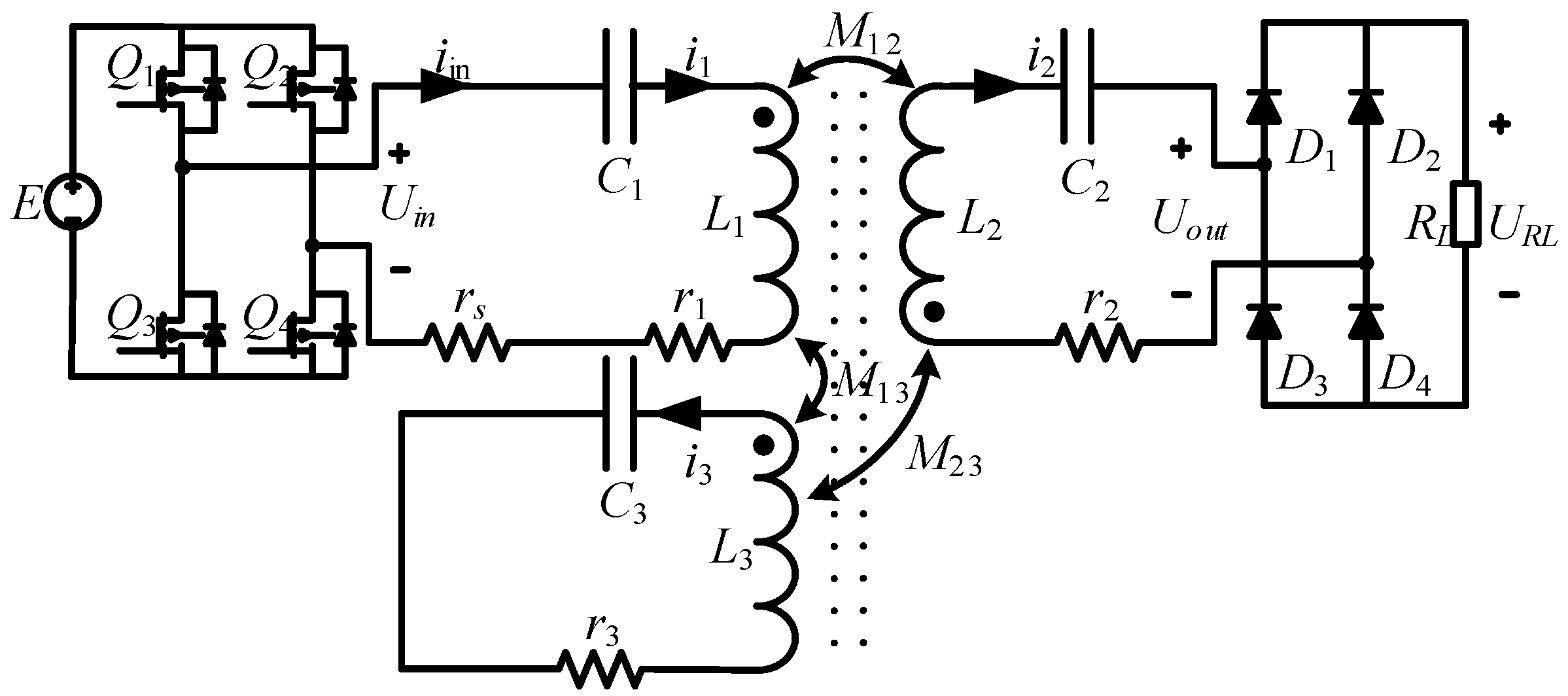
Figure 1 shows the configuration of the proposed series-series compensated 3-coil IPT system. The circuit consists of a constant voltage source E, a full-bridge inverter Q1–Q4 for a square wave generator, a resonant tank including 3 coils: L1, L2, L3 and their resonant capacitor C1, C2, C3, a full-bridge diode rectifier D1–D4 and a load RL. L1, L2 and L3 represent the transmitter coil, the receiver coil and the relay coil, respectively. Mij (i, j = 1, 2, 3, i ≠ j) means mutual-inductance between coil i and coil j.
Based on Figure 1, rs, r1, r2, r3 are the parasite and winding resistance of the source, L1, L2 and L3, respectively. Relationship between the inverter output voltage Uin and the inverter input voltage E is . Relationship between the rectifier input voltage Uout and the load voltage (URL) is .
2.1.1. Equivalent Circuits and Fundamental Analysis
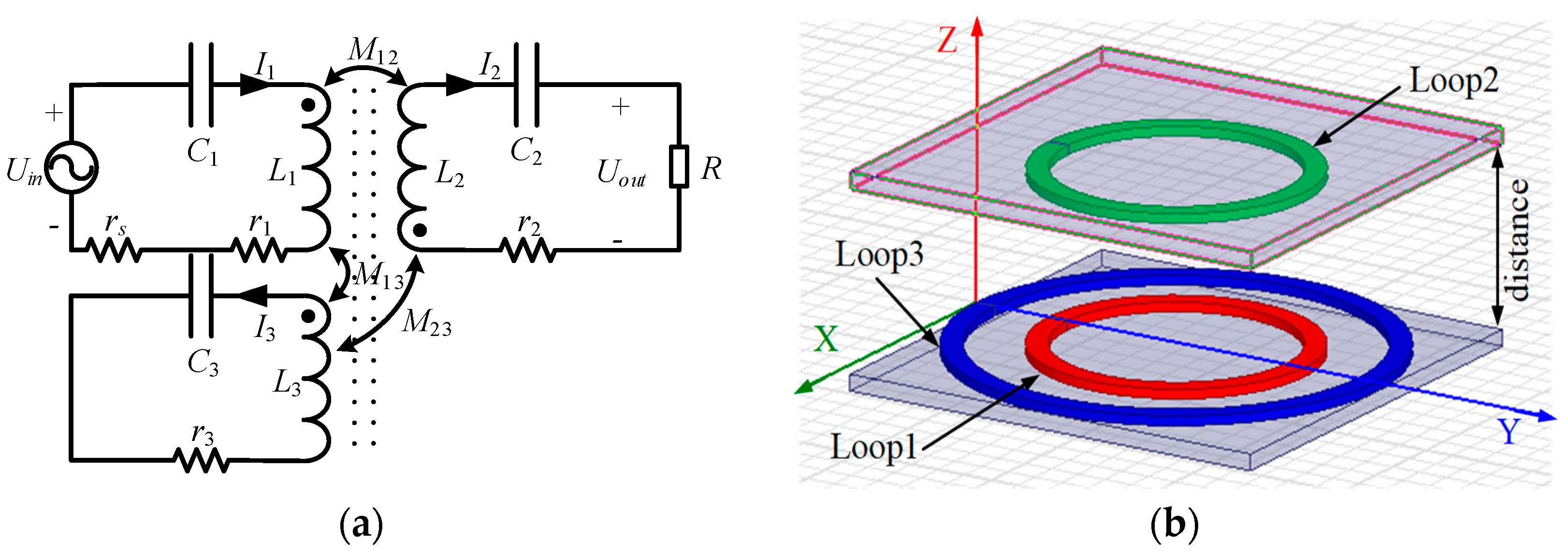
Figure 2 illustrates the resonant tank of the 3-coil system. Transmitter coil and relay coil are placed on a same plane. The geometric design is shown in Figure 2b: the red loop (Loop 1) is the transmitter coil, the green loop (Loop 2) is the receiver coil, the blue loop (Loop 3) is the relay coil, and the two grey square planes are ferrite bars, one below the transmitter and relay coil, and the other one above the receiver coil.
For facilitate analysis, the resonant tank circuit could be described in Equation (1) according to Kirchhoff’s law. In Equation (1), Xi () represents the imaginary component of equivalent impedance for loop i; Ii represents the current flowing through the loop i; ω represents the working efficiency, R represents the equivalent load, as .
2.1.2. Voltage Gain and Methodology for CV Mode
This subsubsection illustrates the voltage gain of the proposed 3-coil system based on Equation (1). The voltage gain GV is defined as the ratio of the output voltage to the input voltage. For simplicity, X1 is set to 0, and the winding resistance ri (i = 1, 2, 3) and rs are neglected, they would be reconsidered in later subsubsection for transfer efficiency.
GV could be calculated as Equation (2), with the current derived from Equation (1).
It is shown in Equation (2) that if the D and B equals 0 simultaneously, GV will not change when the load R varies. Based on this principle, B and D should satisfy Equation (4).
By substituting Equation (4) into Equations (3) and (2), Equation (2) could be rewritten as Equation (5).
It can be seen from the Equation (5) that voltage gain is load-independent now, achieving CV output with Equation (4), X3, which is the imaginary component of the equivalent impedance for loop 3, could be rewritten as Equation (6).
By substituting Equation (6) into Equation Equation (5), GV could be more concise as Equation (7).
Zin, the equivalent impedance of the resonant tank, is defined as the ratio of input voltage to the input current, shown in Equation (8).
are the real part and imaginary part of the input impedance of the resonant tank, respectively. To reduce the system’s power loss, as well as the capacity requirement for the inverter, the Zero Phase Angle (ZPA) condition should be achieved, should be set to 0. After some simple mathematical manipulations, X2, the imaginary component of the equivalent impedance for loop 2, is derived as Equation (9).
Implementing the new X2 value, the equivalent impedance Zin is rewritten as Equation (10).
From Equation (10), it’s obvious that the equivalent impedance of the resonant tank is pure resistive, avoiding the reactive power dissipation caused by inductor or capacitor, achieving ZPA condition and decreasing the system’s power loss and the capacity requirement for the inverter.
Substituting Equation (9) into Equation (6), X3, the imaginary component of the equivalent impedance for loop 3, could be more concise as Equation (11).
Implementing Equation (9) to Equation (7), GV can be rewritten as Equation (12). Notice that as distance between transmitter and receiver coils varies, M23 and M13 also change.
To conclude this subsubsection, if the parameter values satisfy the relationship in Equation (9), (11) as well as , the CV mode could be achieved, as well as ZPA condition. Besides, the GV could be measured with Equation (12).
2.1.3. Efficiency Analysis
This subsubsection illustrates the transfer efficiency for the proposed 3-coil system, with the consideration of the winding resistance ri (i = 1, 2, 3) and the source resistance rs, which are shown in Figure 2.
Figure 2 could be described as the decoupled circuit shown in Figure 3. ra, rb, rc is the reflected impedance from loop 2 to loop 1, from loop 3 to loop 1, from loop 2 to loop 3, respectively, and they are measured in Equation (13).
Based on Figure 3, the transfer efficiency could be derived in Equation (14). represent the efficiency of loop 1, loop 2 and loop 3, respectively.
Transfer efficiency for the whole system is shown in Equation (15), which is the multiplication of the three efficiencies above. The components R1_23, R3_2 in the numerator are illustrated in Equation (16), and R represents the equivalent load, as .
2.1.4. Parameter Value Design
This subsubsection illustrates how to design the parameter values for the proposed 3-coil system. Assuming that the voltage on the dc load RL is URL, and input dc voltage is E, the working efficiency is f and . Based on Equation (12), and the relationship between input voltage and output voltage of the inverter and the rectifier, Equation (17) is derived.
We set and in the experiment of verifying the CV feasibility, where the distance between receiver and transmitter keeps 10 cm. According to Equation (17), the ratio of M23 and M13 is fixed as 0.5. Then the software ANSYS Maxwell (Ozen Engineering, Inc., Silicon Valley, Sunnyvale, CA, USA) is involved to design the coil size to meet , so that the three coils’ size, turns, relative position, self-inductance L1, L2, L3 as well as the mutual-inductance M12 are all determined.
Based on aforementioned requirement , C1 in the transmitter coil is derived in Equation (18).
Based on Equation (11), C3 in the relay coil is derived in Equation (20).
Based on Equation (9), C2 in the receiver coil is shown in Equation (20).
As the capacitor values satisfy Equations (18)–(20), the proposed 3-coil IPT system could achieve CV as well as ZPA condition.
The transfer distance change would lead to differentiation in mutual-inductance, so that the C2 should be recalculated according to Equation (20).
2.2. Parameter Design for S-LCL Compensated 2-Coil System
Besides verifying the feasibility for CV of the aforementioned 3-coil system, a comparison experiment is also needed to prove that the 3-coil system has higher efficiency than that of 2-coil system as distance increasing. The methodology for designing parameter values in 2-coil system is illustrated in this Section 2.2.
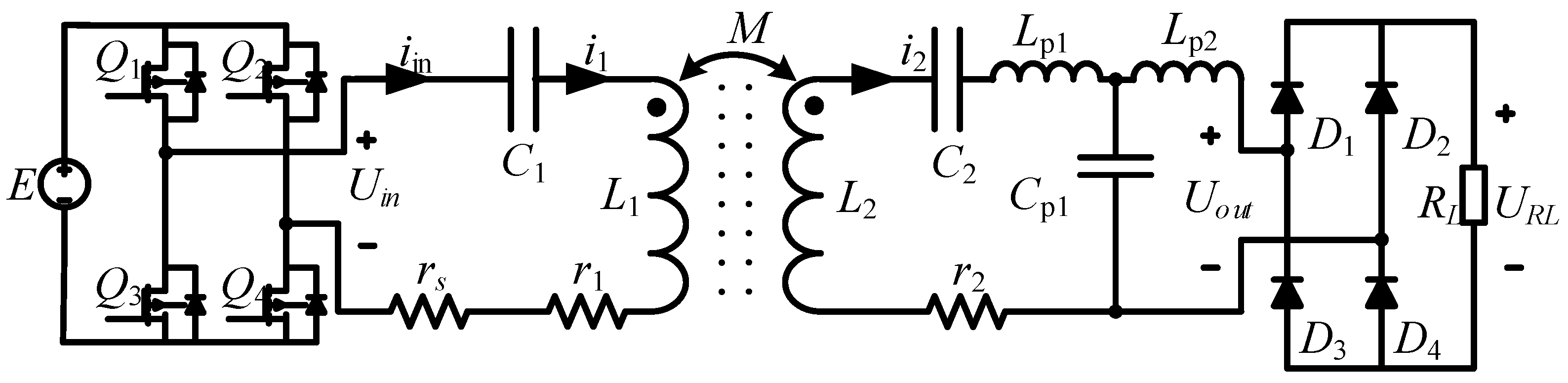
The S-LCL topology of 2-coil circuit is shown in Figure 4.
The voltage gain GV for the 2-coil system shown in Figure 4 could be derived as Equation (21) based on [22].
For a fair and reasonable efficiency-comparing experiment, we adopted the principle mentioned in reference [33]. For a 2-coil system, the power supply drives the transmitter coil and relay coil in series, so that the same copper volume is used in the coupling mechanism for both 2-coil system and 3-coil system. Besides, GV for both systems are designed to be the same value, which varies with transfer distance. GV could be determined with Equation (12).
Based on Equation (22), Inductance values LP1 and LP2 could be measured with Equation (23).
Capacitors C1 and C2 resonant with L1 and L2, respectively. Their values are shown in Equation (24).
If the requirements in Equations (22)–(24) are satisfied, the S-LCL compensated 2-coil system could achieve CV as well as ZPA condition [22].
3. Experimental Analysis
In this experimental part, we firstly build a 3-coil system to test the feasibility for CV. Secondly, with software, we simulate the proposed 3-coil system with the S-LCL 2-coil system, to prove that the former one has higher efficiency as transfer distance changes.
To test the effectiveness of the CV of the 3-coil system, we build an experimental prototype shown in Figure 5a, which includes an oscilloscope (Agilent DSO-X3014T, Santa Clara, CA, USA) to record the experimental output waveforms and a power analyzer (PW6001, HIOKI, Nagano, Japan) to gauge the transfer efficiency between dc source and dc load. The transmitter and receiver coils are wound with Litz wires (0.1 × 400) as shown in Figure 5b. Parameter values are shown in Table 1.
In Figure 5b, loop 1 is the transmitter coil, which connects inverter comprising 4 MOSFETS (C2M0080120D, Cree, Durham, NC, USA); loop 2 is the receiver coil which connects rectifier including 4 diodes (DSEI2X61-06C, IXYS, Milpitas, CA, USA) and the electronic load (IT8518B, ITECH, NanJing, China), loop 3 is the relay coil to generate an enhanced magnetic flux for the power transfer to receiver [19]. For size, the transmitter coil’s outer diameter is 191.5 mm, the same as receiver coil, and the relay coil 300 mm. For relative position, the relay coil and the transmitter coil are remained in the same plane and same centered, the receiver is parallel with the transmitter and same centered; space between relay coil and transmitter is 40 mm, power transfer distance between receiver and transmitter keeps 100 mm in testing the constant voltage output characteristics of the 3-coil system.
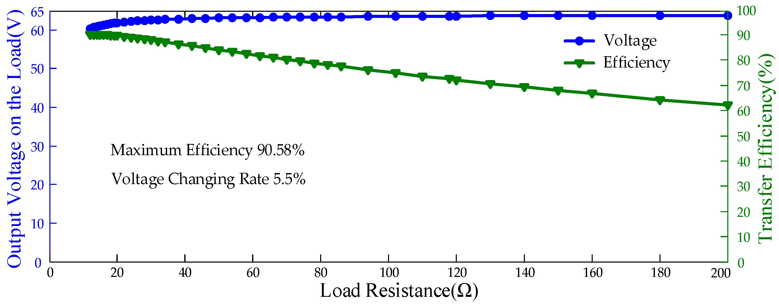
To verify that the output voltage could keep constant as load varies, we change the load from 12 Ω to 200 Ω. Figure 6 shows the DC-DC efficiency and output voltage respectively while load varies.
From Figure 6, the maximum voltage is 63.85 V, the minimum voltage is 60.39 V. Obviously, constant voltage output is achieved with only 5.5% output voltage changing rate as load varies from 12 Ω to 200 Ω. It would show later in Figure 7 that when load varies from 12 Ω to 120 Ω, the voltage changing rate decreases to 5.1%.
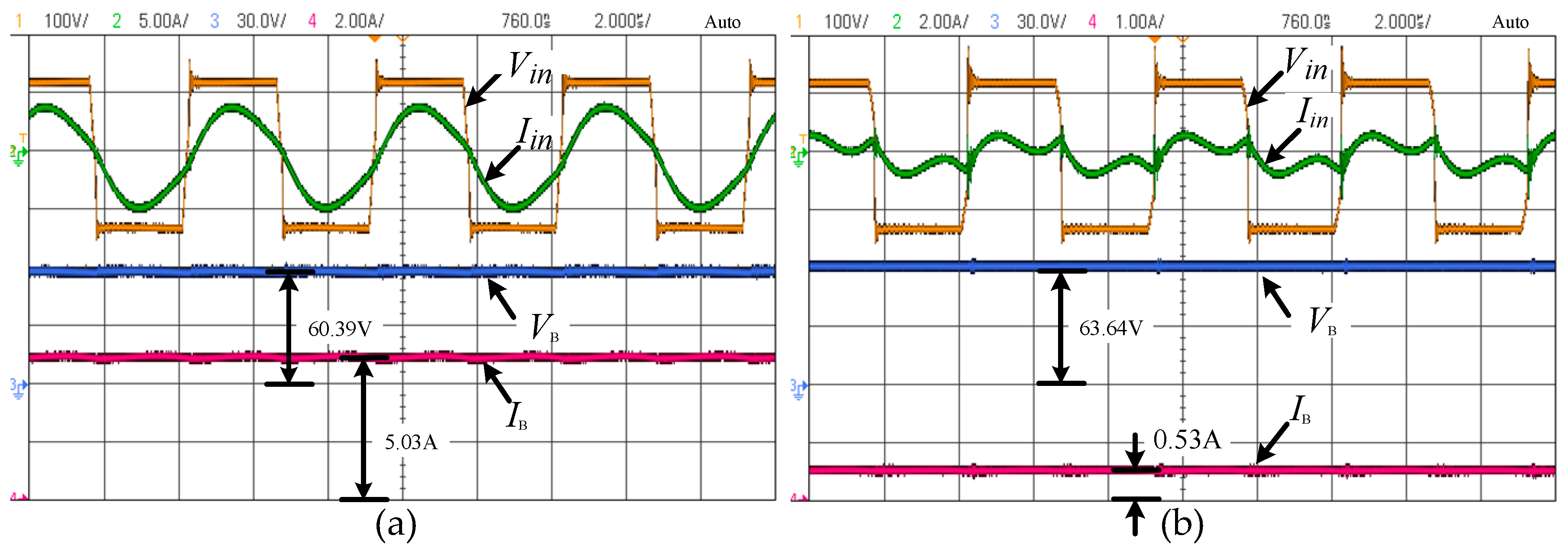
Figure 7 shows the waveforms of voltage Vin output from the inverter, current Iin output from the rectifier, voltage VB on the load, current IB going through the load. Figure 7a shows these waveforms corresponding to 12 Ω, with VB = 60.39 V and IB = 5.03 A, meaning that the output power is 303.76 W, and the transfer efficiency is 90.58%. Figure 7b shows the waveforms corresponding to 120 Ω, with VB = 63.64 V and IB = 0.53 A, meaning that the output power is 33.62 W, and the transfer efficiency is 72.46%. Comparing these two working conditions, we can conclude that the voltage changing rate is 5.1%, almost achieving constant voltage output goal.
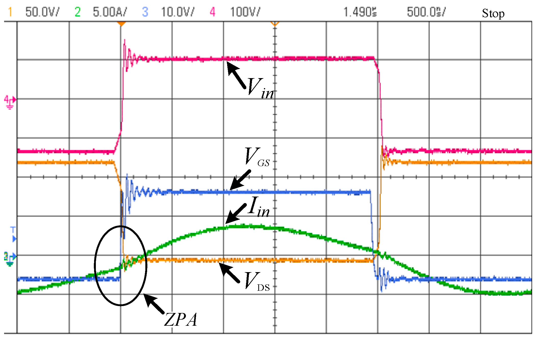
Figure 8 shows the waveforms of the voltage Vin and the current Iin respectively, and the voltage VGS and the voltage VDS between gate and source, drain and source of the MOSFET respectively.
Based on the waveforms of Figure 8, it’s very clear that Vin and Iin correspond simultaneously to the MOSFET gate driving signal: as the MOSFET turn-on signal VGS goes high, VDS and Iin both immediately respond, VDS drops almost to zero as Iin starts flowing from drain terminal to source terminal of the MOSFET, proving that the output voltage Vin and the output current Iin are in the same phase, with no reactive power dissipation.
Figure 9 shows the transient waveforms of Vin and Iin VB and IB respectively, as switching load from 12 Ω to 50 Ω and inversely switching. It’s clear that during the switching period, VB keeps almost constant, and waveforms of Iin and Vin have no obvious overshoot or undershoot, avoiding spike pulse and achieving stability.
To prove that the 3-coil system could relieve efficiency falls better than the 2-coil system, we built an S-LCL compensated 2-coil system simulating model with the resonant tank shown in Figure 4. The magnetic simulations are run in ANSOFT Maxwell (Ozen Engineering, Inc., Silicon Valley, Sunnyvale, CA, USA), getting mutual-inductances and self-inductances. MATLAB/Simulink (2014a, Natick, MA, USA) was used to build the system, which could simulate the current and analyze the efficiency.
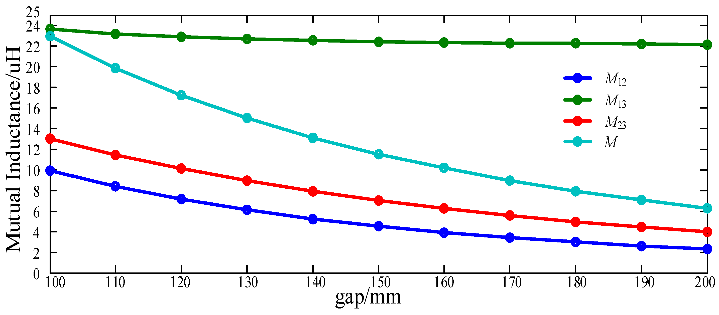
The coupling mechanism for the 3-coil system in Maxwell simulation is shown in Figure 2b. Coupling mechanism of the transmitter side for the 2-coil system is connecting transmitter coil and relay coil in series. Loop 3 and loop 1 is same centered, and the outer diameter for loop 3 is 300 mm, the gap between loop 1 and loop 3 is 40 mm; loop 1 and loop 2 both have 191.5 mm diameter. These 3 coils each has 10 turns, the winding resistance r1, r2, r3 is 0.18 Ω, 0.18 Ω, and 0.29 Ω respectively. Taking 10 mm steps, increasing transfer distance from 100 mm to 200 mm, the mutual-inductance between each coil for both systems got with ANSOFT Maxwell are show in Table 2, where subscription 1, 2 and 3 represent transmitter coil, receiver coil and relay coil, respectively; the changing trend is shown in Figure 10.
To verify that the proposed CV model could reduce efficiency fall when transfer distance increases, we simulate the proposed 3-coil system (shown in Figure 1) and the S-LCL compensated 2-coil system (shown in Figure 4) with MATLAB/Simulink. The requirements for a 3-coil system are: setting the load resistance as 12 Ω, keeping the output voltage as 60 V by manually adjusting the input voltage. The requirements for 2-coil system are: setting the load resistance as 12 Ω, keeping the same input voltage as its 3-coil counterpart, adjusting parameter Lp1, Lp2, and Cp1 to keep 60 V output voltage. The simulation results are shown in Table 3. Where I1, I2 and I3 are the current flowing through transmitter coil, receiver coil and relay coil, respectively.
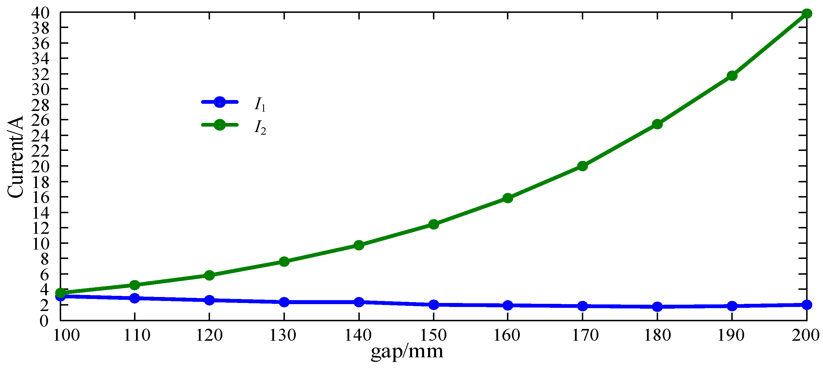
Based on data in Table 3, for the 2-coil system, currents (I1, I2) versus transfer distance are drawn in Figure 11. It’s obvious that as transfer distance increases, I1 decreases firstly, but when the coupling coefficient becomes very week, loss of system becomes excessive large, resulting I1 increases. For I2, it increases from 3.5 A to 39.7 A, leading to increasing loss and decreasing efficiency.
For the 3-coil system, currents (I1, I2, I3) versus transfer distance are drawn in Figure 12. It’s clear that as transfer distance increases, I1 decreases continually, I2 keeps almost constant, and I3 increases from 4.2 A to 11.3 A, leading to lower efficiency but better than that of 2-coil system.
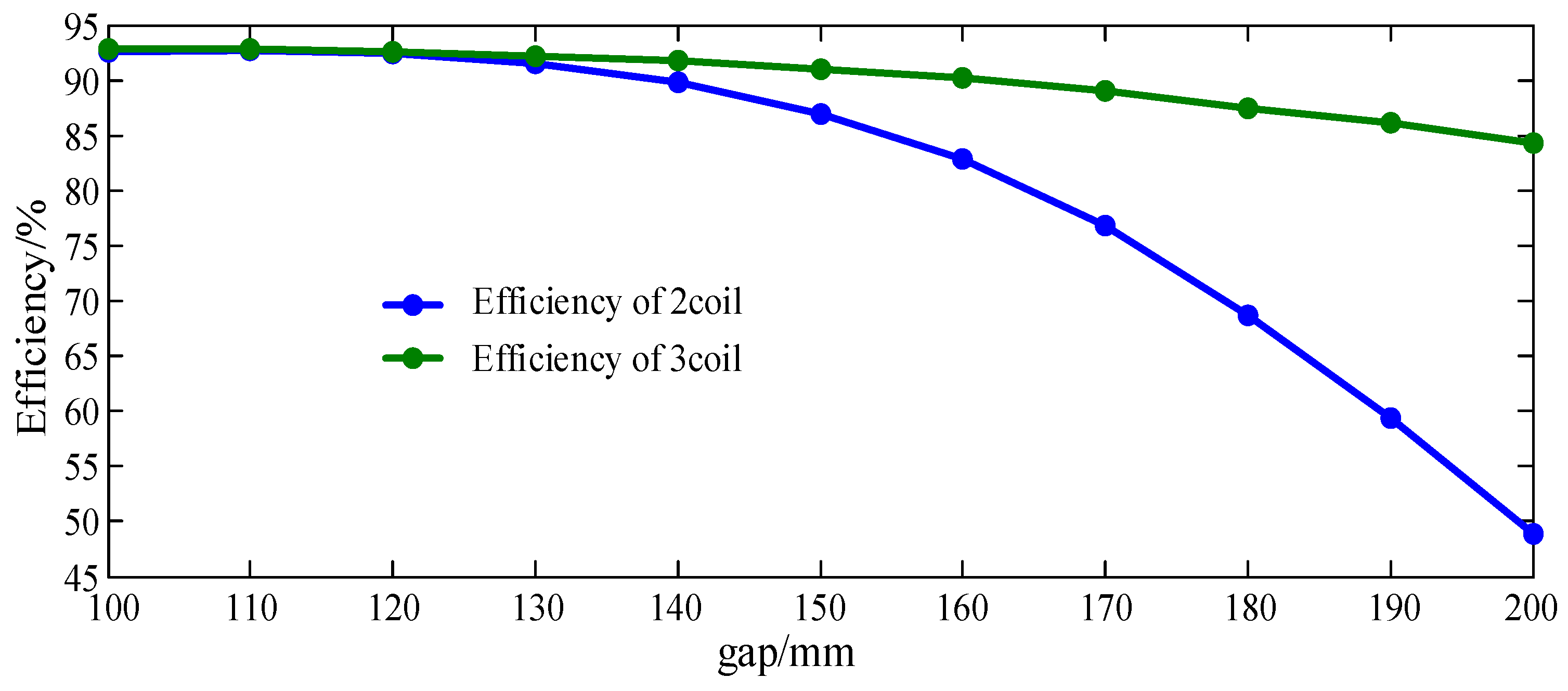
For the two systems, their efficiency trends are shown in Figure 13. It could be seen that as transfer distance increases, the efficiency decreases from 92.61 to 48.9% for the 2-coil system, and it decreases from 92.89 to 84.26% for the 3-coil system. Proving that the proposed model could improve the transfer efficiency as power transfer distance increases.
4. Conclusions
This essay proposes a SS compensated 3-coil IPT system to achieve CV and ZPA conditions, solving the efficiency decreasing problem in long distance coupling for the traditional 2-coil IPT system. This proposal has no complicated control circuit, and the output voltage only involves the ratio of mutual-inductances between the coils. In the CV verification experiment, the voltage change rate is 5.5% as the load varies from 12 Ω to 200 Ω, with 100 mm transfer distance. In the simulated comparing experiment, as transfer distance increases from 10 cm to 20 cm, transfer efficiency for 2-coil system decreases from 92.61 to 48.9%, for 3-coil system from 92.89 to 84.26%. The experiment results prove that the proposed prototype could achieve CV and that the 3-coil system has a higher efficiency than the 2-coil system when increasing transfer distance. Thus, the proposal is feasible and effective to achieve CV as well as ZPA conditions.
Acknowledgments
This paper was supported by National Key R&D Program of China (2017YFB1201002), the National Natural Science Foundation of China under Grant (No. 51677155), the Sichuan Youth Science & Technology Foundation (No. 2016JQ0033), the Fundamental Research Funds for the Central University (No. 2682017QY01).
Author Contributions
Ruikun Mai and Yang Chen proposed the main idea. Youyuan Zhang designed and performed the experiment. Ruimin Dai wrote the paper. All the authors have read and approved the final manuscript.
Conflicts of Interest
The authors declare no conflict of interest.
References
- Zhang, X.; Yang, Q.; Chen, H.; Li, Y.; Cai, Y.; Jin, L. Modeling and Design and Experimental Verification of Contactless Power Transmission Systems via Electromagnetic Resonant Coupling. Proc. CSEE 2012, 32, 153–158. (In Chinese) [Google Scholar]
- González-González, J.M.; Triviño-Cabrera, A.; Aguado, J.A. Design and Validation of a Control Algorithm for a SAE J2954-Compliant Wireless Charger to Guarantee the Operational Electrical Constraints. Energies 2018, 11, 604. [Google Scholar] [CrossRef]
- Liu, Y.; Hu, A.P. Study of Power Flow in an IPT System Based on Poynting Vector Analysis. Energies 2018, 11, 165. [Google Scholar] [CrossRef]
- Fan, X.; Mo, X.; Zhang, X. Research Status and Application of Wireless Power Transmission Technology. Proc. CSEE 2015, 35, 2584–2600. (In Chinese) [Google Scholar]
- Li, Y.; Mai, R.; Lu, L.; He, Z. Active and Reactive Currents Decomposition based Control of Angle and Magnitude of Current for a Parallel Multi-Inverter IPT System. IEEE Trans. Power Electron. 2017, 32, 1602–1614. [Google Scholar] [CrossRef]
- Hu, G.; Zhang, J.; Wang, J.; Fang, Z.; Cai, C.; Lin, Z. Combination of Compensations and Multi-Parameter Coil for Efficiency Optimization of Inductive Power Transfer System. Energies 2017, 10, 2088. [Google Scholar] [CrossRef]
- Lu, F.; Zhang, H.; Mi, C. A Review on the Recent Development of Capacitive Wireless Power Transfer Technology. Energies 2017, 10, 1752. [Google Scholar] [CrossRef]
- Mai, R.; Li, Y.; He, Z.; Yang, M.; Lu, L.; Liu, Y.; Chen, Y.; Lin, T.; Xu, D. Wireless Power Transfer Technology and Its Research Progress In Rail Transportration. J. Southwest Jiaotong Univ. 2016, 51, 446–461. (In Chinese) [Google Scholar]
- Sallán, J.; Villa, J.L.; Llombart, A.; Sanz, J.F. Optimal Design of ICPT Systems Applied to Electric Vehicle Battery Charge. IEEE Trans. Ind. Electron. 2009, 56, 2140–2149. [Google Scholar] [CrossRef]
- Mai, R.; Ma, L. Research on Inductive Power Transfer Systems with Dual Pick-up Coils. Proc. CSEE 2016, 36, 5192–5199. (In Chinese) [Google Scholar]
- Fareq, M.; Fitra, M.; Irwanto, M.; Syafruddin, H.S.; Gomesh, N.; Farrah, S.; Rozailan, M. Solar wireless Power Transfer Using Inductive Coupling for Mobile Phone Charger. In Proceedings of the 2014 IEEE 8th International Power Engineering and Optimization Conference (PEOCO2014), Langkawi, Malaysia, 24–25 March 2014; pp. 473–476. [Google Scholar]
- Xu, W.; Liang, W.; Peng, J.; Liu, Y.; Wang, Y. Maximizing Charging Satisfaction of Smartphone Users via Wireless Energy Transfer. IEEE Trans. Mob. Comput. 2017, 16, 990–1004. [Google Scholar] [CrossRef]
- Kang, W.; Alexander, Z.; Jun, H.; Park, Y.; Pack, J. Exposure Assessment for a Wireless Multi-Phone Charger. In Proceedings of the 2014 International Symposium on Electronmagnetic Compatibility, Tokyo, Japan, 12–16 May 2014; pp. 198–201. [Google Scholar]
- Chung, E.; Lee, J.; Ha, J. System Conditions Monitoring Method for a Wireless Cellular Phone Charger. In Proceedings of the 2014 International Power Electronics and Application Conference and Exposition, Shanghai, China, 5–8 November 2014; pp. 639–643. [Google Scholar]
- Li, H.; Li, J.; Wang, K.; Chen, W.; Yang, X. A maximum Efficiency Point Tracking Control Scheme for Wireless Power Transfer Systems Using Magnetic Resonant Coupling. IEEE Trans. Power Electron. 2015, 30, 3998–4008. [Google Scholar] [CrossRef]
- Mai, R.; Zhang, Y.; Chen, Y.; Kou, Z.; He, Z. Study on IPT Charging System with Hybrid Topology for Configurable Charge Currents. Proc. CSEE 2017. (In Chinese) [Google Scholar] [CrossRef]
- Boys, J.T.; Covic, G.A.; Xu, Y. DC Analysis Technique for Inductive Power Transfer Pick-ups. IEEE Power Electron. Lett. 2003, 1, 51–53. [Google Scholar] [CrossRef]
- Vu, V.B.; Doan, V.T.; Pham, V.L.; Choi, W. A new method to implement the constant Current-Constant Voltage charge of the Inductive Power Transfer system for Electric Vehicle applications. In Proceedings of the IEEE Transportation Electrification Conference and Expo, Busan, Korea, 1–4 June 2016; pp. 449–453. [Google Scholar]
- Wu, H.H.; Gilchrist, A.; Sealy, K.D.; Bronson, D. A High Efficiency 5 kW Inductive Charger for EVs Using Dual Side Control. IEEE Trans. Ind. Inform. 2012, 8, 585–595. [Google Scholar] [CrossRef]
- Mai, R.; Chen, Y.; Liu, Y. Compensation Capacitor alteration Based IPT Battery Charging Application with Constant Current and Constant Voltage Control. Proc. CSEE 2016, 36, 5816–5821. (In Chinese) [Google Scholar]
- Mai, R.; Chen, Y.; Zhang, Y.; Li, Y.; He, Z. Study on Secondary Compensation Capacitor alteration Based IPT Charging System. Proc. CSEE 2017, 33, 3263–3269. (In Chinese) [Google Scholar]
- Mai, R.; Chen, Y.; Li, Y.; Zhang, Y.; Cao, G.; He, Z. Inductive Power Transfer for Massive Electric Bicycles Charging Based on Hybrid Topology Switching with A Single Inverter. IEEE Trans. Power Electron. 2017, 8, 5897–5906. [Google Scholar] [CrossRef]
- Kiani, M.; Jow, U.M.; Ghovanloo, M. Design and optimization of a 3-coil inductive link for efficient wireless power transmission. IEEE Trans. Biomed. Circuits Syst. 2011, 5, 579–591. [Google Scholar] [CrossRef] [PubMed]
- Tran, D.H.; Vu, V.; Choi, W. Design of a High Efficiency Wireless Power Transfer System with Intermediate Coils for the On-board Chargers of Electric Vehicles. IEEE Trans. Power Electron. 2017, 1, 175–187. [Google Scholar] [CrossRef]
- Kurs, A.; Karalis, A.; Moffatt, R.; Joannopoulos, J.D.; Fisher, P.; Soljacic, M. Wireless power transfer via strongly coupled magnetic resonances. Science 2007, 317, 83–86. [Google Scholar] [CrossRef] [PubMed]
- Beh, T.C.; Kato, M.; Imura, T.; Oh, S.; Hori, Y. Automated Impedance Matching System for Robust Wireless Power Transfer via Magnetic Resonance Coupling. IEEE Trans. Ind. Electron. 2013, 60, 3689–3698. [Google Scholar] [CrossRef]
- Zhong, W.X.; Zhang, C.; Liu, X.; Hui, S.Y.R. A Methodology for Making a Three-Coil Wireless Power Transfer System More Energy Efficient Than a Two-Coil Counterpart for Extended Transfer Distance. IEEE Trans. Power Electron. 2015, 30, 933–942. [Google Scholar] [CrossRef]
- Moon, S.; Kim, B.C.; Cho, S.Y.; Ahn, C.H.; Moon, G.W. Analysis and design of a wireless power transfer system with an intermediate coil for high efficiency. IEEE Trans. Ind. Electron. 2014, 61, 5861–5870. [Google Scholar] [CrossRef]
- Kim, J.W.; Son, H.C.; Kim, K.H.; Park, Y.J. Efficiency analysis of magnetic resonance wireless power transfer with intermediate resonant coil. IEEE Antennas Wirel. Propag. Lett. 2011, 10, 389–392. [Google Scholar] [CrossRef]
- Zhang, F.; Hackworth, S.A.; Fu, W.; Li, C.; Mao, Z.; Sun, M. Relay effect of wireless power transfer using strongly coupled magnetic resonances. IEEE Trans. Magn. 2011, 47, 1478–1481. [Google Scholar] [CrossRef]
- Moon, S.; Moon, G.W. Wireless Power Transfer System with an Asymmetric Four-Coil Resonator for Electric Vehicle Battery Chargers. IEEE Trans. Ind. Electron. 2016, 31, 6844–6854. [Google Scholar]
- Ahn, D.J.; Hong, S.C. A study on magnetic field repeater in wireless power transfer. IEEE Trans. Ind. Electron. 2013, 60, 360–371. [Google Scholar] [CrossRef]
- Kamineni, G.; Covic, A.; Boys, J.T. Analysis of Coplanar Intermediate Coil Structures in Inductive Power Transfer Systems. IEEE Trans. Power Electron. 2015, 30, 6141–6154. [Google Scholar] [CrossRef]
Figure 1.
Configuration of the proposed series-series compensated 3-coil IPT (inductive power transfer) system.
Figure 1.
Configuration of the proposed series-series compensated 3-coil IPT (inductive power transfer) system.

Figure 2.
Resonant tank in (a) equivalent circuits model (b) 3D module in Maxwell.

Figure 3.
Decoupled circuit of resonant tank for the proposed 3-coil system.
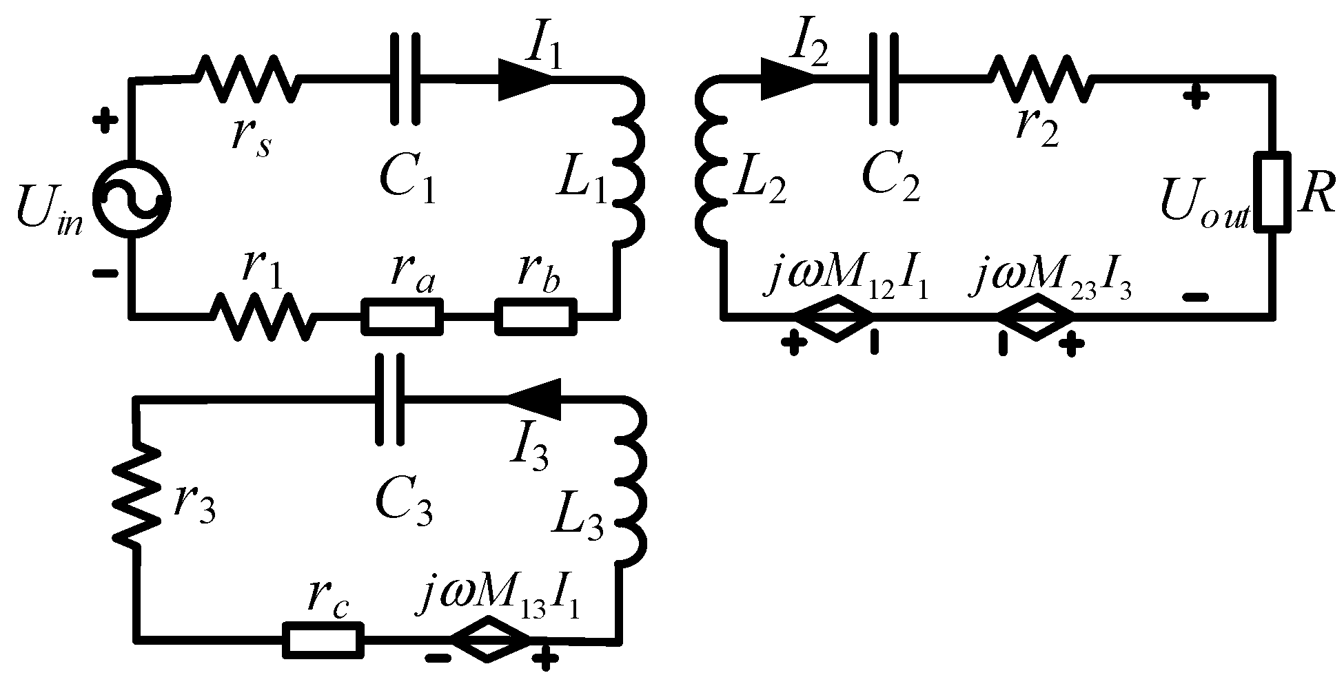
Figure 4.
S-LCL compensated 2-coil system from [22].
Figure 4.
S-LCL compensated 2-coil system from [22].

Figure 5.
(a) Prototype of the 3-coil system (b) Resonant tank of the 3-coil system.
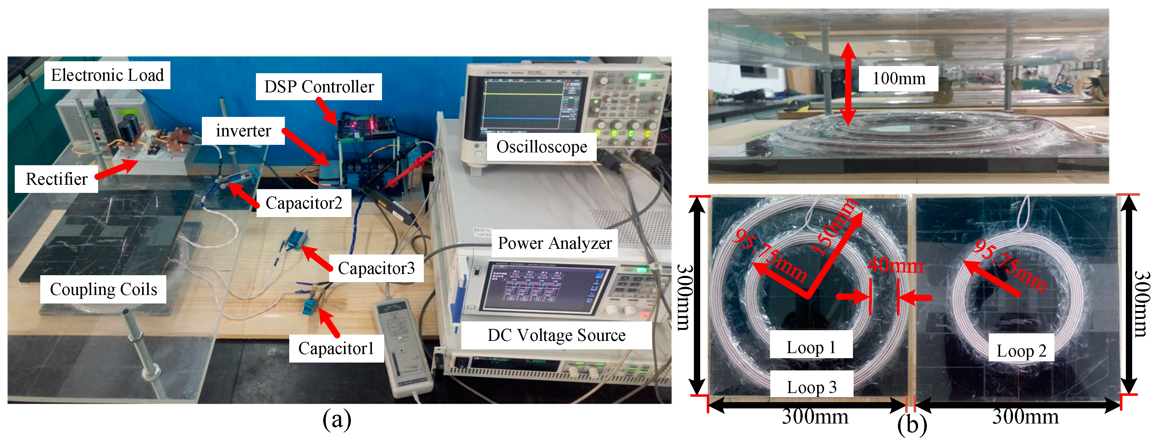
Figure 6.
Output voltage and efficiency respectively versus load resistance for the 3-coil system.

Figure 7.
Experimental waveforms of Vin, Iin, VB, IB at (a) (b) .

Figure 8.
Experimental waves of Vin, Iin, VDS, VGS.

Figure 9.
The transient waveforms of Vin, Iin, VB, IB when the load switches between 12 Ω and 50 Ω.
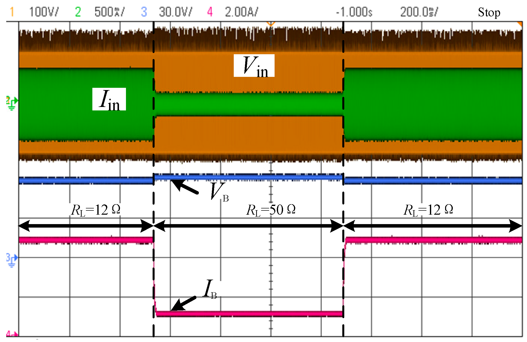
Figure 10.
Mutual-inductance Versus Transfer distance.

Figure 11.
Current Versus Transfer Distance for 2-coil System.

Figure 12.
Current Versus Transfer Distance for 3-coil System.
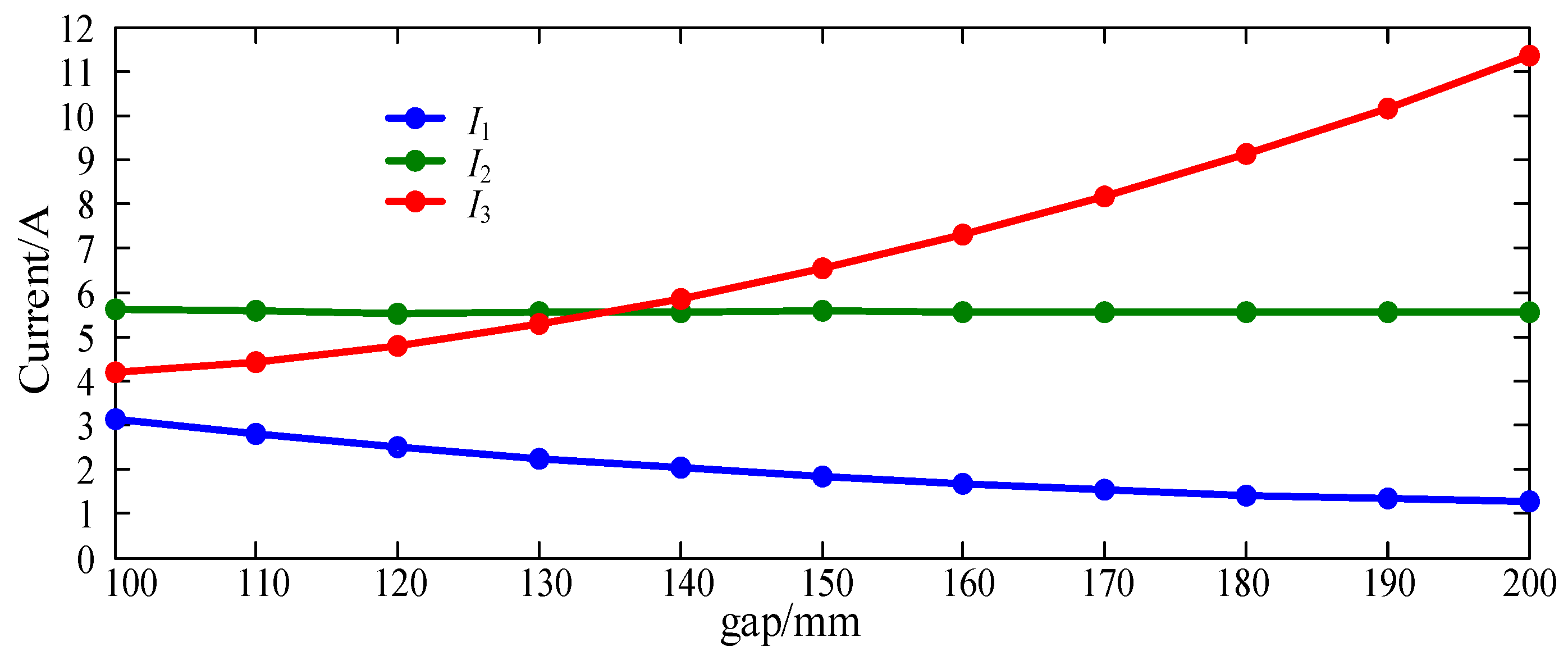
Figure 13.
Mutual-inductance Versus Transfer Distance.


Table 1.
Parameter values for 3-coil system.
| Parameter | Value | Parameter | Value |
|---|---|---|---|
| Frequency f/kHz | 200 | Capacitor C2/nF | 13.681 |
| Input voltage E/V | 120 | Capacitor C3/nF | 6.701 |
| Self-inductance L1/uH | 53.76 | Transfer distance gap/mm | 100 |
| Self-inductance L2/uH | 56.69 | Outer radius of Loop 1 R1/mm | 95.75 |
| Self-inductance L3/uH | 94.497 | Outer radius of Loop 2 R2/mm | 95.75 |
| Mutual inductance M12/uH | 9.5425 | Outer radius of Loop 3 R3/mm | 150 |
| Mutual inductance M13/uH | 23.255 | Number of turns for Loop 1 N1 | 10 |
| Mutual inductance M23/uH | 12.675 | Number of turns for Loop 2 N2 | 10 |
| Capacitor C1/nF | 11.779 | Number of turns for Loop 3 N3 | 10 |
Table 2.
Parameters for coupling mechanism for both systems.
| Model | gap/mm | 100.00 | 110.00 | 120.00 | 130.00 | 140.00 | 150.00 | 160.00 | 170.00 | 180.00 | 190.00 | 200.00 |
|---|---|---|---|---|---|---|---|---|---|---|---|---|
| 3 coil | L1/uH | 62.51 | 62.23 | 61.94 | 61.87 | 61.73 | 61.64 | 61.49 | 61.54 | 61.54 | 61.46 | 61.56 |
| L2/uH | 62.57 | 62.35 | 61.96 | 61.98 | 61.82 | 61.61 | 61.57 | 61.73 | 61.65 | 61.71 | 61.61 | |
| L3/uH | 107.14 | 106.82 | 106.20 | 106.26 | 105.53 | 105.54 | 105.57 | 105.37 | 105.25 | 105.42 | 105.32 | |
| M12/uH | 9.93 | 8.38 | 7.13 | 6.09 | 5.23 | 4.52 | 3.92 | 3.41 | 2.98 | 2.61 | 2.30 | |
| M13/uH | 23.66 | 23.20 | 22.91 | 22.71 | 22.51 | 22.40 | 22.34 | 22.27 | 22.28 | 22.19 | 22.16 | |
| M23/uH | 13.04 | 11.46 | 10.09 | 8.92 | 7.88 | 7.00 | 6.23 | 5.55 | 4.96 | 4.44 | 3.98 | |
| 2 coil | L1/uH | 216.98 | 215.45 | 213.96 | 213.54 | 212.29 | 211.99 | 211.75 | 211.46 | 211.34 | 211.27 | 211.19 |
| L2/uH | 62.57 | 62.35 | 61.96 | 61.98 | 61.82 | 61.61 | 61.57 | 61.73 | 61.65 | 61.71 | 61.61 | |
| M/uH | 22.97 | 19.84 | 17.22 | 15.00 | 13.11 | 11.52 | 10.16 | 8.96 | 7.94 | 7.05 | 6.28 |
Table 3.
Simulating result.
| Model | gap/mm | 100.00 | 110.00 | 120.00 | 130.00 | 140.00 | 150.00 | 160.00 | 170.00 | 180.00 | 190.00 | 200.00 |
|---|---|---|---|---|---|---|---|---|---|---|---|---|
| 3 coil | Pin/w | 329.80 | 325.70 | 323.10 | 326.40 | 327.60 | 331.90 | 332.60 | 336.10 | 344.40 | 347.70 | 356.20 |
| Pout/w | 306.30 | 302.20 | 299.20 | 301.10 | 300.70 | 301.90 | 300.10 | 299.10 | 301.30 | 299.60 | 300.10 | |
| η/% | 92.89 | 92.78 | 92.62 | 92.24 | 91.79 | 90.96 | 90.24 | 88.99 | 87.50 | 86.15 | 84.26 | |
| URL/V | 60.62 | 60.22 | 59.92 | 60.11 | 60.07 | 60.19 | 60.01 | 59.91 | 60.13 | 59.96 | 60.01 | |
| E/V | 117.20 | 129.50 | 144.10 | 161.80 | 181.00 | 203.00 | 226.50 | 253.00 | 284.00 | 315.00 | 351.00 | |
| I1/A | 3.13 | 2.80 | 2.50 | 2.25 | 2.03 | 1.84 | 1.67 | 1.53 | 1.42 | 1.33 | 1.27 | |
| I2/A | 5.61 | 5.58 | 5.53 | 5.57 | 5.56 | 5.57 | 5.56 | 5.55 | 5.57 | 5.55 | 5.56 | |
| I3/A | 4.21 | 4.43 | 4.78 | 5.28 | 5.87 | 6.56 | 7.30 | 8.16 | 9.14 | 10.17 | 11.34 | |
| 2 coil | Pin/w | 325.00 | 324.20 | 325.40 | 328.40 | 334.60 | 345.50 | 362.30 | 390.80 | 435.80 | 504.50 | 613.60 |
| Pout/w | 301.00 | 300.50 | 300.70 | 300.70 | 300.70 | 300.50 | 300.10 | 300.20 | 299.30 | 299.30 | 300.20 | |
| η/% | 92.61 | 92.69 | 92.41 | 91.57 | 89.87 | 86.98 | 82.81 | 76.81 | 68.67 | 59.33 | 48.92 | |
| URL/V | 60.10 | 60.05 | 60.07 | 60.07 | 60.07 | 60.05 | 60.01 | 60.02 | 59.93 | 59.93 | 60.02 | |
| E/V | 117.20 | 129.50 | 144.10 | 161.80 | 181.00 | 203.00 | 226.50 | 253.00 | 284.00 | 315.00 | 351.00 | |
| I1/A | 3.12 | 2.82 | 2.55 | 2.33 | 2.33 | 2.01 | 1.88 | 1.80 | 1.76 | 1.81 | 1.96 | |
| I2/A | 3.53 | 4.54 | 5.86 | 7.58 | 9.74 | 12.47 | 15.81 | 20.04 | 25.41 | 31.76 | 39.75 |
© 2018 by the authors. Licensee MDPI, Basel, Switzerland. This article is an open access article distributed under the terms and conditions of the Creative Commons Attribution (CC BY) license (http://creativecommons.org/licenses/by/4.0/).
Share and Cite
MDPI and ACS Style
Mai, R.; Zhang, Y.; Dai, R.; Chen, Y.; He, Z. A Three-Coil Inductively Power Transfer System with Constant Voltage Output. Energies 2018, 11, 673. https://doi.org/10.3390/en11030673
AMA Style
Mai R, Zhang Y, Dai R, Chen Y, He Z. A Three-Coil Inductively Power Transfer System with Constant Voltage Output. Energies. 2018; 11(3):673. https://doi.org/10.3390/en11030673
Chicago/Turabian StyleMai, Ruikun, Youyuan Zhang, Ruimin Dai, Yang Chen, and Zhengyou He. 2018. "A Three-Coil Inductively Power Transfer System with Constant Voltage Output" Energies 11, no. 3: 673. https://doi.org/10.3390/en11030673
Note that from the first issue of 2016, this journal uses article numbers instead of page numbers. See further details here.