Availability of Ambient RF Energy in d-Dimensional Wireless Networks

1
State Key Laboratory of Integrated Service Network, Xidian University, Xi’an 710071, China
2
Department of Electrical and Computer Engineering, Kansas State University, Manhattan, KS 66506, USA
*
Author to whom correspondence should be addressed.
†
Current address: School of Computer and Information Science, Hubei Engineering University, Xiaogan 432000, China.
Energies 2018, 11(3), 668; https://doi.org/10.3390/en11030668
Submission received: 23 February 2018
/
Revised: 11 March 2018
/
Accepted: 13 March 2018
/
Published: 15 March 2018
(This article belongs to the Section F: Electrical Engineering)
Abstract
:Radio frequency (RF) enabled energy harvesting has garnered increasingly broad applications in energy-constrained wireless networks. In this context, the actual available energy is constrained by the harvesting threshold of RF harvesters. In this paper, we first propose two new metrics, effective energy harvesting probability (EEHP) and spatial mean harvestable energy (SMHE) to characterize the availability of ambient RF energy. Assuming that the transmitters are spatially distributed according to a d-dimensional homogeneous Poisson point process (HPPP), we derive the distributions of the ambient RF energy for networks, from the perspective of information receivers, with and without interference control (IC). The corresponding EEHP and SMHE are given in integral forms for the case with IC and inverse Laplace transform form for the case without IC, respectively. For a special case where the dimension to path loss ratio equals 0.5, closed-form exact/approximate expressions for EEHP and SMHE are derived. Analytical results are validated by Monte Carlo simulations. Numerical results with distinct network parameters indicate that the harvesting threshold always has a significant effect on the EEHP, while the impact on SMHE can be ignored as the transmitter density increases. The general unified framework considered in this paper expands the applicability of the derived results to arbitrary dimensional networks.
1. Introduction
Wireless networks with energy-constrained nodes typically have a limited lifetime severely limiting their sustained application [1]. RF energy harvesting is becoming a promising approach to power such energy-constrained wireless nodes. Specifically, RF energy harvesting capability allows wireless devices to exploit energy from radio signals for their information transmission. RF enabled wireless powered communications (WPC) is attracting increasing interest in many domains, especially in wireless sensor networks and the Internet of Things (IoT) [2]. As radio signals are quite weak (due to exponentially decaying path loss effects), improving energy harvesting efficiency finds broad acceptance and new applications. To this end, possible approaches include: (i) shortening the distance between the transmitter and RF energy harvesting node and (ii) exploiting co-channel interference from other access points (APs) (usually named ambient RF energy) as energy sources. Fortunately, dense large scale wireless networks (LSWN) like urban vehicle ad hoc networks and future 5G cellular networks may meet these two requirements [3]. These networks provide wireless devices the opportunity to harvest energy in sufficiently short distance and/or accumulate possibly more energy from nearby transmitters.
RF energy harvesting in large-scale networks has been analyzed in [4,5,6,7,8]. In the inspiring work of [4], opportunistic energy harvesting in cognitive radio networks has been studied where the secondary users harness the energy radiated by nearby active primary transmitters. In [5], simultaneous information and energy transfer with feasible power control strategy have been studied in large scale networks without/with relaying, under constraints of average harvested-energy and outage probability. In [6], the feasibility of simultaneous information and energy transfer in LTE-A small cell networks was discussed, the energy harvesting performance was maximized subject to information transfer constraint. Che et al. propose a harvest-then-transmit protocol for WPC networks by partitioning each frame into a downlink phase for energy transfer, and an uplink phase for information transfer [7]. By jointly optimizing frame allocation strategy and the transmit power, the wireless nodes’ spatial throughput is maximized. The performance of network coding-aided cooperative communications in large scale networks is studied [8], where the relays are powered by RF energy.
In the trade-off design of WPC, the evaluation of energy harvesting performance is critical. There are two main challenges in this endeavor. The first challenge involves the accurate modeling of the harvested-energy, which is closely related to the path loss model and the channel fading model. In [4,7], taking into account its tractability, an unbounded path loss (UBPL) model is employed to analyze the amount of harvested-energy. However, the UBPL model suffers from the issue of infinite harvested energy when the transmitters get arbitrarily close to the receiver. While this singularity can be ignored in relatively sparse networks [9], the harvested-energy would be overestimated in denser networks. The path loss model adopted in [5] is bounded and nonsingular, yet it only formulates the average harvested-energy over the plane, and it is insufficient to analyze the performance of individual nodes. The second major challenge in quantifying performance is the availability analysis of the harvested-energy. The root of this challenge lies in the fact that only the RF power that exceeds a certain threshold can be harvested (due to the harvester’s circuit limits [4,10]). This factor is considered by defining a harvesting zone around the transmitter in [4]. It is important to note that, in a dense network, it is also possible for nodes located at the intersection of transmission ranges of adjacent APs harvest enough energy to exceed the harvesting threshold.
1.1. Related Works
There have been some recent efforts on quantifying energy harvesting capacity in large scale networks. Most of these works adopt stochastic geometry tools to model and analyse the RF energy harvested from randomly located transmitters. The two most important network models are Ginibre -determinantal point process (DPP) [11] and homogeneous Poisson point process (HPPP) [12,13,14,15,16], due to their mathematical tractability. Besides, the channel model (including large and small scale fading) also affects the harvesting performance. We summarize and present a comparison of system models and the associated performance results presented in related works in Table 1.
In [11], the mean RF energy harvesting rate was characterized and the upper bound of power outage probability was derived without considering small scale fading. A K-tier HPPP cellular model accompanying with Rayleigh fading channel was investigated in [12]. The CDF of RF energy was leveraged to evaluate the uplink transmission probability and the coverage probability of cellular users. To study the energy efficiency of wireless-powered cellular networks, authors of [16] derived the closed-form mean of RF energy for BPL and Rayleigh channel model. Instead of modeling transmitters as infinite PPP, the authors of [13] used a set of a finite annulus with PPP distributed nodes to model the transmitter locations. The CDF of incident power was formulated and represented by an infinite series. In [15], the mmWave energy harvesting performance was studied in the network where power beacons and energy harvesting nodes both constitute a PPP. Considering BPL and Nakagami fading model, the CDF of RF energy was obtained by integrating the Gamma function. Other than mmWave base stations, the work of [14] also investigated the RF energy harvesting capacity for Sub-6GHz small cellular networks. The CDF of RF energy from sub-6GHz and mmWave base stations were both presented in integral form.
1.2. Contributions
In this paper, by modeling the transmitter positions as a d-dimensional homogeneous Poisson point process (HPPP), we investigate the availability of the ambient RF energy at a typical point in a large scale wireless network. The availability includes two aspects: the effective energy harvesting probability (EEHP) and the spatial mean harvestable energy (SMHE). The former is defined as the probability that the harvested-energy of a node exceeds harvesting threshold, which indicates the effectiveness of the incident power. The latter indicates the average available energy over the entire space. To remove the singularity of UBPL model, we adopt a bounded path loss (BPL) model and get finite mean of the RF energy. Another distinct aspect of this work that differentiates it from prior efforts is that we consider a multidimensional model which has not been investigated in RF energy harvesting. Beyond conventional 2-D network [11,12,13,14,15,16], the analysis under the multidimensional model can find wide applications for 1-D vehicle networks [17,18], as well as 3-D wireless sensor networks [19,20,21].
Furthermore, in determining whether a node can harvest energy from transmitters other than the nearest one, we will study the networks with and without interference control (IC), respectively. It is worth noting that the term interference control comes not from the perspective of energy harvesters, but instead from the information receivers. With IC techniques like directive antennas, OFDM or MAC layer scheduling, the concurrent transmitters use orthogonal radio resources to communicate with their associated users, or the transmitters are far enough that the interference to each other is negligible [22]. Thus, in networks with IC, we only calculate the energy harvested from the nearest transmitter. On the contrary, in the system without IC, we consider the cumulative effect of received energy from all transmissions.
In summary, the key contributions of our work include:
- By modeling transmitters as a d-dimensional large-scale network, we derive the mean and the CDF of the harvested-energy under BPL and Rayleigh fading model using tools from stochastic geometry. The networks with and without interference control are separately considered. Our unified framework is general and the derived results can be applied to 1-D, 2-D and 3-D networks.
- Considering the practical constraint imposed by the RF harvesting circuit, we propose two metrics: the EEHP and the SMHE to measure the availability of the ambient RF energy. Other works like [11] have proposed metric such as power outage probability. However, the threshold they refer to in their work is the circuit power consumption, not the suggested turn-on power of the harvester (considered in this paper).
- We derive compact expressions for the CDF and mean of the RF harvested energy including some closed-form expressions for a special case (which is practical in the real environment). The numerical method to calculate the RF energy distribution is given. To gain insight into the results, we derive and analyze the lower bound of distribution function and the upper bound of the mean. These results can be readily used to evaluate the communication capacity of wireless powered nodes.
- We validate the theoretical analysis with Monte Carlo simulations. The proposed bounds of the EEHP and the SMHE for different settings are verified. We show that while the harvesting threshold has a significant effect on the EEHP, it has a negligible impact on the SMHE, especially for dense networks. Also, we illustrate that in terms of improving the SMHE, the increase of transmitter density is more efficient than increasing transmit power. Last but not the least, we show that interference control has a trivial effect on RF energy harvesting performance for a sparse network; Since the performance of LSWN-IC and LSWN-noIC is comparable in sparse networks, the mathematically tractable expressions for SMHE and EEHP for LSWN-IC can serve as surrogate metrics to analyze LSWN-noIC.
The rest of this paper is organized as follows. The system model and the performance metrics are described in Section 2. In Section 3, the EEHP and the SMHE in LSWN-IC are formulated and derived. Section 4 presents the availability analysis of LSWN-noIC. Finally, the simulation results and discussions are presented in Section 5 before the paper is concluded in Section 6.
2. System Model and Performance Metrics
2.1. System Model
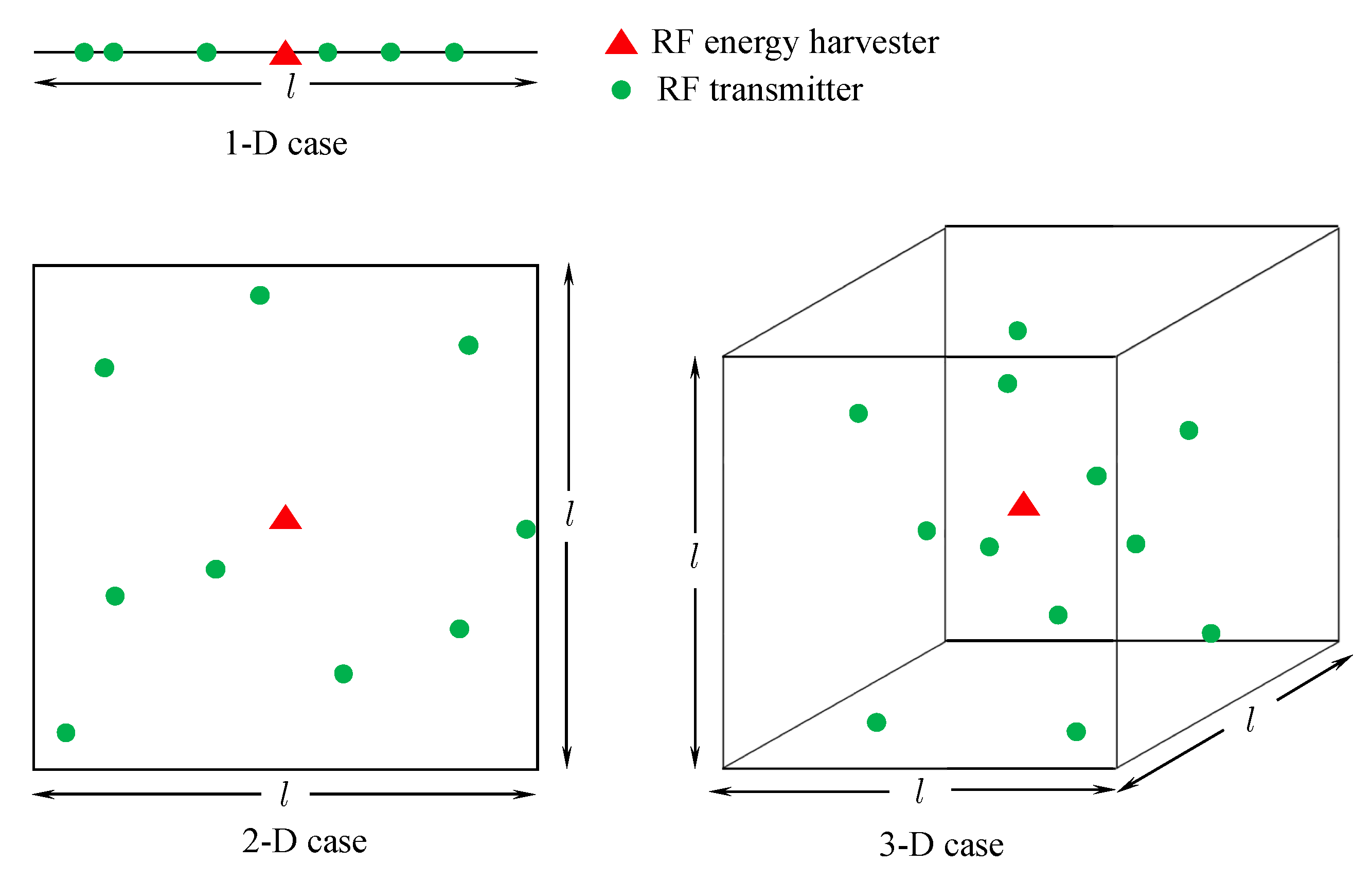
We assume that the position of receiver (Rx), , follows a d-dimensional HPPP with density , i.e., . In addition, we also assume that the position of the transmitter (Tx), , follows a d-dimensional HPPP with density , i.e., ; We will also use and to refer to the node itself. According to Slivnyak-Mecke Theorem, the reduced Palm distribution of a PPP is equal to its original distribution [23]. Therefore, without loss of generality, we assume that the origin is the typical position of energy harvesters. The spatial models of the 1-D [17], 2-D [24] and 3-D [21] network are depicted in Figure 1. For the 1-D case, the transmitters are placed on the line according to a HPPP with density (in ), the RF energy harvester is located in the middle of the segment of length l. For the 2-D case, the nodes within a square of side length l are distributed according to HPPP with dentiy (in ), the RF energy harvester is located in the center of the square. For the 3-D case, the transmitters’ position follow HPPP with density (in ) within a cube of side length l, the RF energy harvester is situated in the center of the cube.
According to Friis formula, the received power of Rx at distance z from the transmitter in free space is [25]:
where is transmitting power, is received power, z is the T-R distance, is the system loss factor, and is the wavelength. To simplify the expression, we formulate all the factors in Formula (1) into an equivalent transmit power , where that excludes the distance factor . Considering a general path loss exponent (, ) and the effect of small scale fading, the received RF signal power at the origin based on a signal emitted by transmitter is given by
where denotes the Euclidean distance between point and the origin. The symbol denotes the channel fading coefficient. Note that the case may occur as the position of transmitter is random. In addition, this will result in the received power to be larger than the transmitting power violating the law of conservation of energy. To prevent this case, we adopt the bounded path loss (BPL) model following [26], where,
The received power at the origin from the transmitter is given as
The received power at the origin accumulated from all the transmitters over the entire space then corresponds to
where denotes the set of concurrent transmitters in the same frequency band.
In this paper, we consider two types of networks. For large-scale wireless networks with interference control (LSWN-IC), we assume that the harvesting node always chooses the nearest AP as its transmitter, denoted by , and the power radiated by other transmitters can be ignored. We state that this model can simulate networks well with directive energy harvesting, which has higher energy harvesting efficiency [14,27]. For omni-directive energy harvesting, as shown in Section 5.2, the analysis with IC also gives a compact bound for networks without IC with lower computation cost. For the large-scale wireless networks without interference control (LSWN-noIC), we assume the node can harvest RF energy from all the transmitters over the entire space. Then the set in (5) can be expressed as,
Note that for the case that partial transmitters are scheduled to use the same frequency band to avoid interference, like ALOHA protocol with transmit probability p, the set of concurrent transmitters forms a PPP with intensity . This follows from the independent thinning property of the PPP [26]. We can just replace the density (in case that all APs transmitting) by and the follow of results retain the same form.
To simplify the harvesting energy availability analysis, we assume that all transmitters use the same transmit power as . Without loss of generality, we assume all the wireless links experience independent Rayleigh fading with unit mean. Integrating the equivalent transmit power and channel fading effect, we get the equivalent channel gain as , which follows an Exponential distribution with parameter , i.e.,
Based on the above assumption, (5) can be simplified as
2.2. Metrics of Availability
We propose two indexes measuring the availability of RF energy harvested from randomly deployed Txs: effective energy harvesting probability (EEHP) and spatial mean harvestable energy (SMHE) that are defined below.
Definition 1.
Effective energy harvesting probability refers to the probability that the received power of the energy harvester exceeds the harvesting threshold Θ. That is,
where is the CDF of the received power.
Remark 1.
For large-scale networks consisting of randomly located receivers, the EEHP can be viewed as the average ratio of chargeable receivers’ number to non-chargeable ones’. This metric indicates how many receivers in a large scale network can benefit from the RF energy radiated by randomly located transmitters. Also, this metric implies the probability that the typical receiver could be charged with a given threshold.
The harvesting threshold determines the EEHP. Lower the threshold , higher the achievable EEHP. The typical value of is between −20 dBm and 30 dBm, which depends on specific rectenna and operational frequency [28].
Definition 2.
Spatial mean harvestable energy refers to the mean energy harvested by all the nodes in a d-dimensional space which consists of PPP distributed transmitters (In this paper, without loss of generality, we assume the coherence time or the energy harvesting duration is unit time. Therefore we will not differentiate the word power and energy. Sometimes we may use them interchangeably.). That is,
where denotes the probability density function (PDF) of the received power, is the energy harvesting efficiency for input power x.
Remark 2.
SMHE indicates how much energy can be actually used in the networks. This metric measures the RF energy transfer capability from a system perspective.
The energy harvesting efficiency depends on the input power, matched networks, operational frequency, etc. [29]. It is hard to describe in a unified formula, and it is also beyond the scope of this study. Therefore, we assume the power conversion efficiency is for all input power levels. Then, the expression of SMHE simplifies to
Equations (9) and (11) illustrate that the above two indices to measure availability can be derived from the distribution of the received power, . In Section 3, we will directly evaluate the received power distribution for LWSN-IC. For LWSN-noIC, we will derive the received power distribution by using inverse Laplace transform, as shown in Section 4.
3. RF Energy Harvesting in LSWN-IC
In this section, we will first derive the received power distribution at the origin in LSWN-IC. Then we will calculate the mean harvestable energy. To directly interpret the effect of system parameters (like network density and channel fading) on RF energy harvesting performance, we will derive exact expression for EEHP and an upper bound of SMHE for a special case.
3.1. Distribution of Received Power
We denote as the received power at the origin in LSWN-IC. From (8) we get
where is the position of the nearest transmitter to the receiver. The distance between to the origin is assumed to be , the CDF of which is given as [30]:
where is the volume of a d-dimensional unit ball ( can be expressed in terms of gamma function as ), is the density of the network. Then we obtain the CDF of the received power as follows,
Proposition 1.
The CDF of received power at the typical point in a d-dimensional PPP network with IC is
where , the symbol denotes dimension to path loss ratio.
Proof of Proposition 1.
Let , then Proposition 1 is proved. ☐
Considering the special case of , e.g., the path loss exponent to be 4 within 2-dimensional space, we can get the semi-closed-form expression for the CDF of the received energy. By using the result [31]
where is the complementary error function, we obtain the following Lemma,
Lemma 1.
For , the CDF of the incident power at a typical receiver is
Introducing in Definition 1, we arrive at the expression for EEHP in LSWN-IC.
Proposition 2.
For a given harvesting threshold Θ, the Effective Energy Harvesting Probability of a typical receiver in LWSN-IC is
where the integration can be numerically calculated. For special case of , there is an exact form corresponding to,
3.2. Spatial Mean Harvestable Energy
We now calculate the SMHE of LSWN-IC for a given harvesting threshold .
Proposition 3.
The Spatial Mean Harvestable Energy of PPP distributed receivers in LSWN-IC is
where .
Proof of Proposition 3.
According to Definition 2, the SMHE over d-dimensional space in LSWN-IC is:
Since the distribution of the channel fading gain and the receiver position are independent, the expectation of the received power can be obtained as
We note that the SMHE consists of two parts. Only the second part involves the harvesting threshold. Thus the first part can be seen as the upper bound of SMHE as
4. RF Energy Harvesting in LSWN-noIC
Due to the presence of infinite summation, the received power distribution is hard to derive directly in LSWN-noIC. In this part, we first obtain the Laplace Transform (LT) of the received power via mapping theorem and then get the distribution of the received power by Inverse Laplace Transform (ILT). Lastly, the EEHP and the SMHE is evaluated.
4.1. Laplace Transform of the Received Power
We use a method similar to the analysis of shot noise process to obtain the distribution of the received power [32]. Firstly, by mapping theorem, the d-dimensional homogeneous PPP with density can be mapped to a one-dimensional in-homogeneous PPP with density , where
The received power at the origin in LSWN-noIC, according to (8) , can be given as
The Laplace transform of is defined as follows:
Before continuing, we restate a known result from interference analysis of a finite Poisson network [33].
Corollary 1.
The Laplace transform of the interference at the typical node in a finite homogeneous Poisson network with density λ is:
where
Symbol A and B denotes the inner and outer radius of a finite Poisson network, respectively. In addition, is the upper incomplete Gamma function.
In light of Corollary 1 , we obtain the Laplace function of the received power at the origin as
The total received power can be computed as the sum of two terms : (1) ,the power received from the transmitters within d-dimensional unit sphere, and (2) , the power accumulated from all transmitters at distances greater than 1. As the transmitters follow PPP, the and the are independent. By applying and (bounded path loss model) to (28), we get as follows:
The corresponding function for is the case that and , then
Note that the first item of converges to only when . Fortunately, this condition is always met in real life. Then the Laplace function of the received power is:
By introducing
and
(refer to 6.445.1 in [31], where is the hypergeometric function) into (32), we then get the following proposition.
Proposition 4.
Laplace function of the received power at the typical point in LSWN-noIC is
4.2. Distribution of Received Power
We compute probability distribution of the received power by inverse Laplace transform of [34], i.e.,
While there is no closed-form expression for (36), we can use the Euler inverse Laplace algorithm to get a numerical solution [35]. In particular, we assume a real valued function with Laplace function , then can be computed as
Here, M is used to adjust the calculation precision.
Although this numerical algorithm can give an approximate distribution of the incident power at a typical receiver, the effect of system parameters (like transmitter density or transmitting power) on energy harvesting performance cannot be intuitively observed. It is known that for the dimension to path loss ratio being 0.5, the closed-form CDF of the received power exists [24]. To this end, we derive a compact lower bound with a closed-form for . We will show in Section 5 that this bound is tight in the low power regime.
Lemma 2.
(Lower bound for the CDF of with ). Assuming the channels follow Rayleigh fading with expectation , the transmitters form a PPP with density , the dimension to path loss ratio is 0.5, the CDF of the incident power of a typical receiver is lower bounded by
Proof of Lemma 2.
Suppose that the incident power under UBPL model is , the probability that the incident power for UBPL model is greater than a given x cannot be less than that for BPL model, as shown in (41). That is because, under UBPL model, the transmitter can be deployed boundlessly close to the receiver, which results in higher incident power in a statistical sense. Thus,
or equivalently,
According to Corollary 1 , the UBPL model implies that the inner radius is 0 and the outer radius is infinity. Introducing , into (28), we get Laplacian of as:
Having obtained CDF of the received power, it is straight forward to derive the EEHP for a given harvesting threshold using Definition 1. As EEHP is just the CCDF of the received power with parameter , it is unnecessary to restate the conclusion. Accordingly, we can get the upper bound of EEHP for case from Lemma 2 as follows
where is the error function.
4.3. Spatial Mean Harvestable Energy
Proposition 5.
Assuming that all the links between transmitters and receivers follow Rayleigh fading with unit expected power, the spatial mean harvestable energy of receivers over a PPP network is:
where Θ represents the harvesting threshold, is given by (35)
Proof of Proposition 5.
From (11), we get
Expression (a) is the average received power ignoring the harvester’s sensitivity. We calculate (a) by two parts, one part is the average power radiated by transmitters within the unit sphere. Another part comes from the transmitters outside the unit sphere. The mean of is given by .
To evaluate the mean of , we resort to the corollary from [33] that gives the nth cumulant of interference power for a Poisson network as follows:
Replacing B with ∞ and A with 1, we get . As and are independent,
As has no closed-form, one can employ numerical Laplace inverse to calculate (b).
where (51) is integrated by parts. in (52) denotes the Laplace transform of . In light of temporal integration property, . ☐
Let the threshold tends to 0, we obtain the upper bound of the SMHE as
For case , we can obtain an accurate approximation to SMHE, which will be verified in Section 5, as follows
Lemma 3.
(Approximation to SMHE for case ). If δ equals 0.5, the SMHE under harvesting threshold Θ can be approximated as,
where .
Proof of Lemma 3.
To be shown by simulations in Section 5, the CDF bound of RF power given in Lemma 2 is compact. Thereby, we replace approximately by , then the expression (b) in (47) can be given by
5. Simulation Results and Discussion
In this section, we first verify the proposed numerical or exact results by Monte Carlo simulations in Section 5.1. Then, in Section 5.2, we illustrate the impact of network parameters: transmit power and transmitter density, on the energy harvesting performance using numerical methods.
5.1. Verifying the Proposed Analysis Framework
To confirm the proposed analysis framework, we simulate large scale 2-D and 3-D Poisson networks without/with IC in Matlab. The Tx-Rx channel gains are independent and identically distributed (IID) Rayleigh fades with unit mean. The transmit power is set to 30 dBm. The energy harvesting efficiency is set to 1. The network parameters are listed in Table 3, where L denotes side length of the square (for 2-D model) or of the cube (for 3-D model); N denotes the realization times of fading channels for every implementation of Poisson network. For 2-D ultra dense networks, the density of access points ranges from [36], while for 4G cellular networks the density of base stations approaches 0.0001 in the city of London [37]. To gain an sight into the energy harvesting performance in a dense and a sparse network, we set the density to 0.1 and 0.0001, respectively.
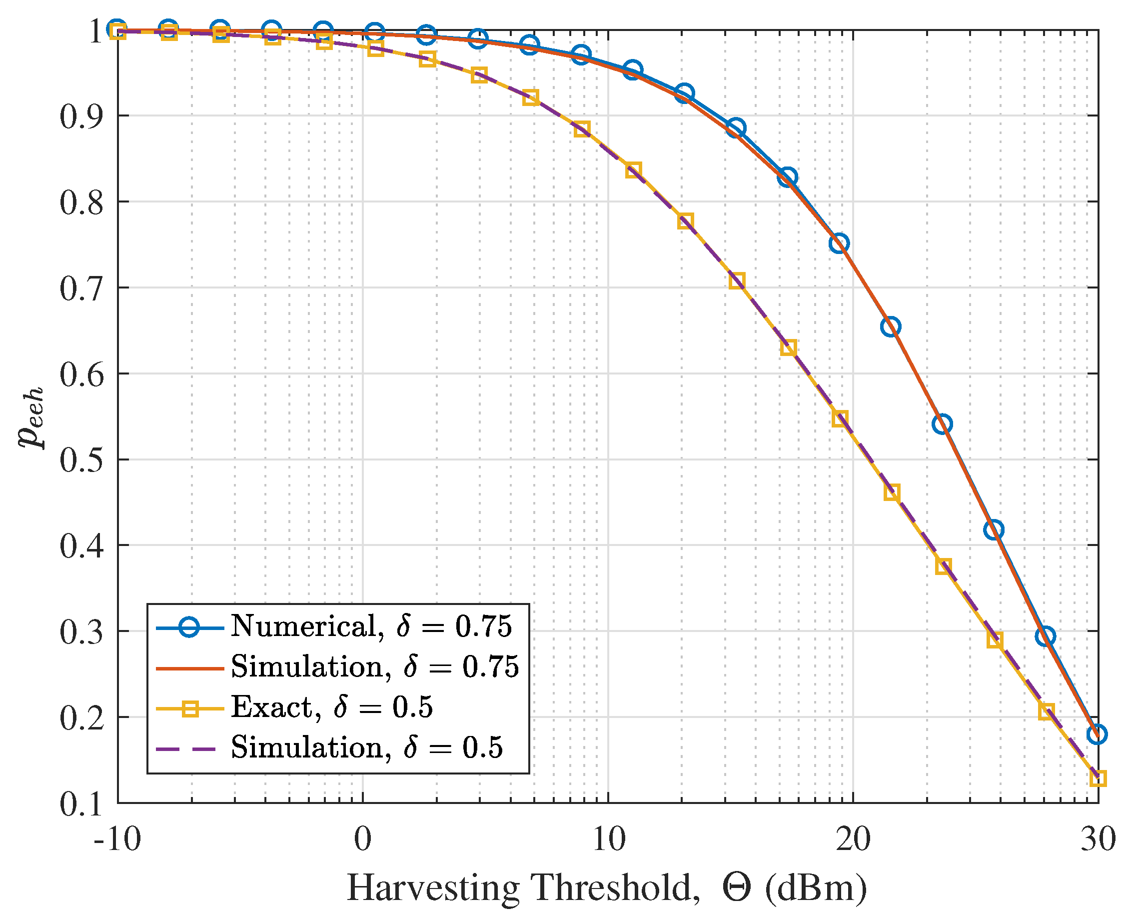
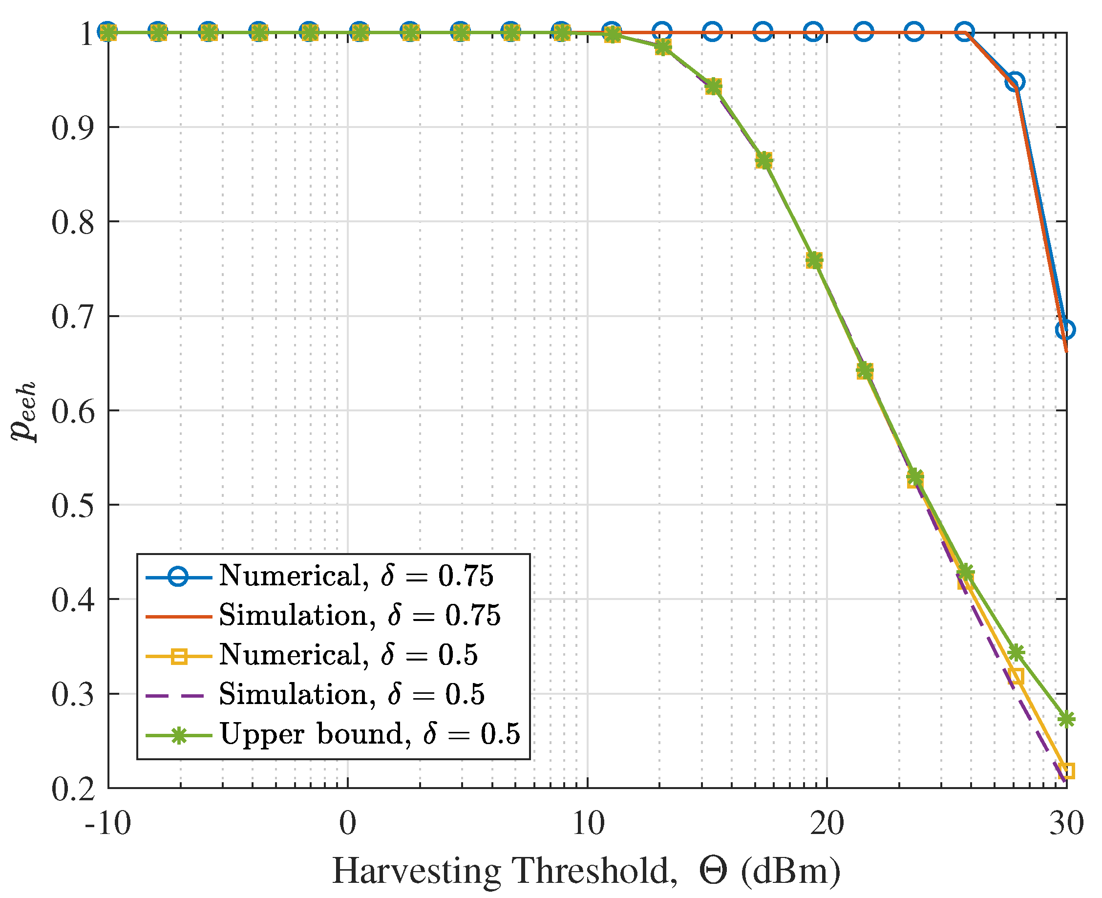
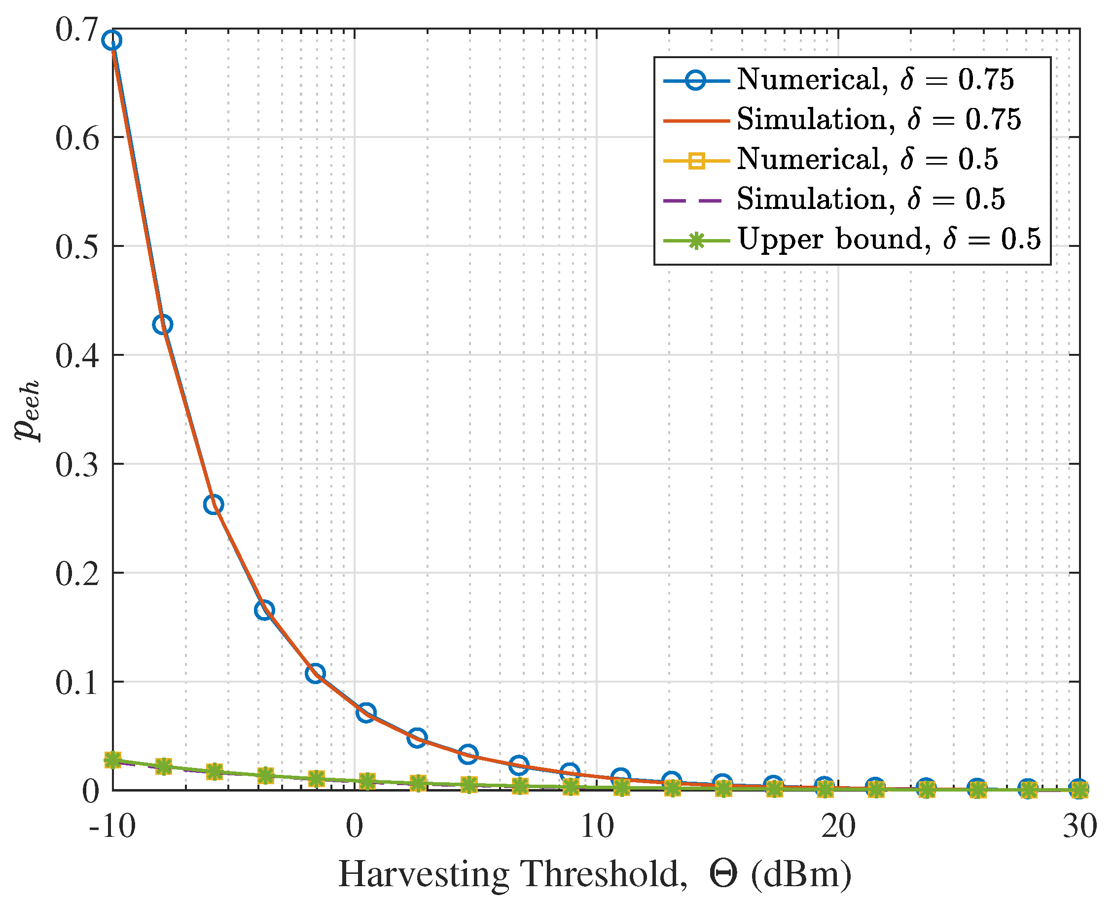
In Figure 2, we plot the simulation and the numerical results of EEHP for a dense large scale network with interference control. The transmitter density is set to . The performance is presented in 2-D and 3-D network with path loss exponent 4. The simulation and analysis curves match well validating our theoretical results. The same outcome can be observed for a sparse network with density , as shown in Figure 3. However, as expected, the EEHP for a sparse network is much lower than for a dense one. In Figure 4 and Figure 5, we compare the simulated EEHP and the numerical result for LSWN-noIC with transmitter density and , respectively. It is seen that relative to LSWN-IC, the EEHP for LSWN-noIC is significantly higher. This result is consistent with our intuition, as for case without IC, more transmitters contribute to the accumulation of RF energy at the receiver. Besides, the upper bound is shown to be extremely compact, especially for a low-density network.
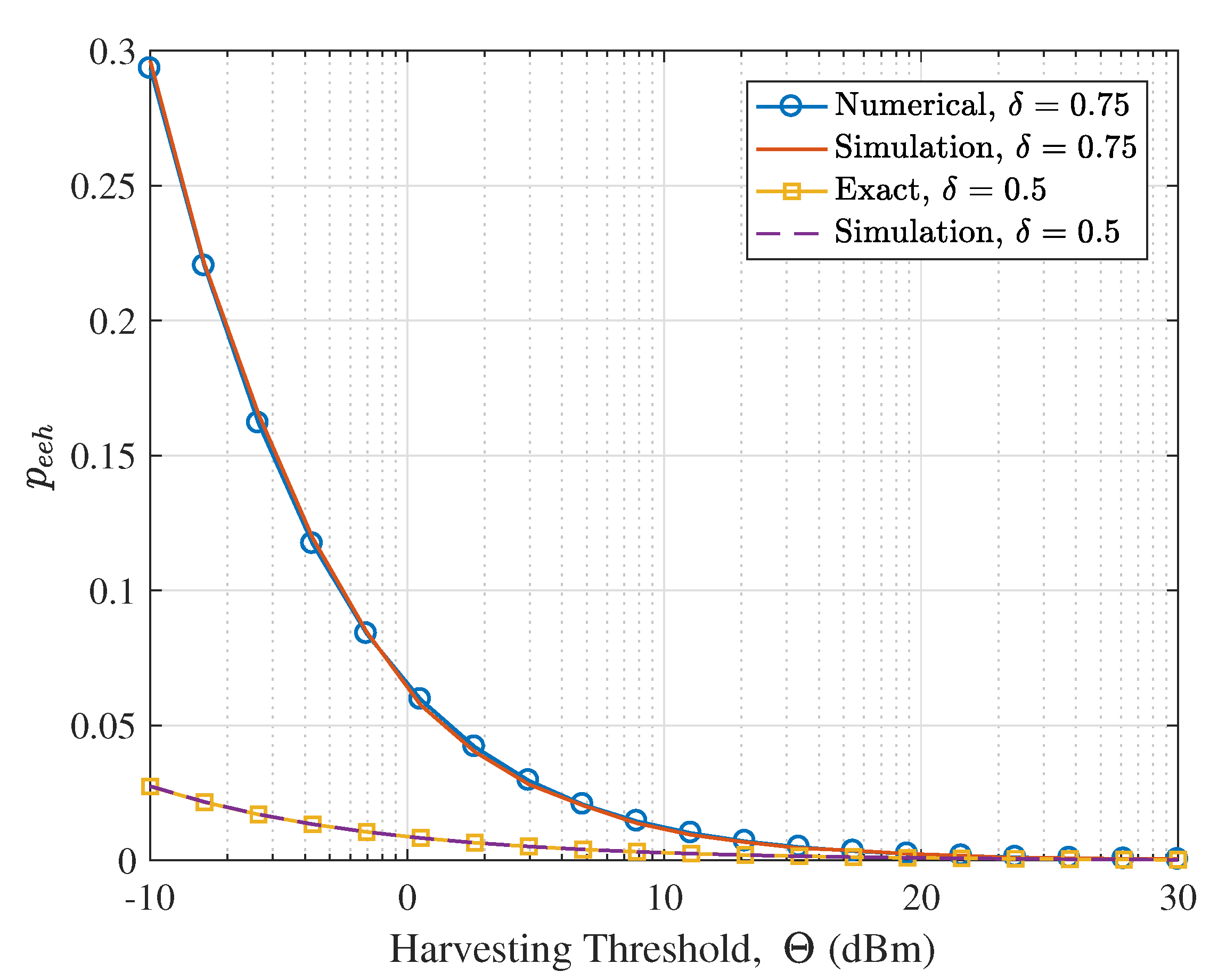
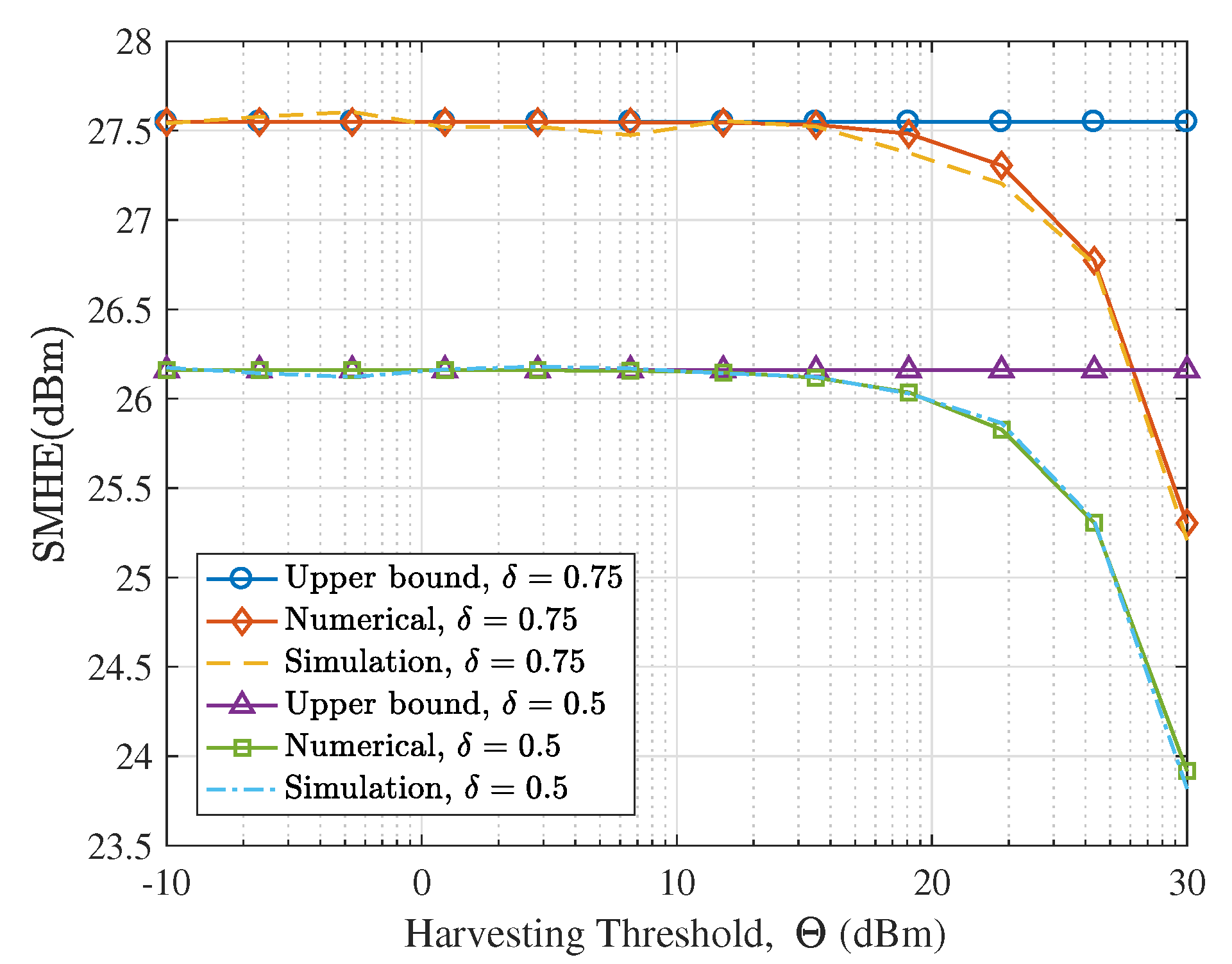
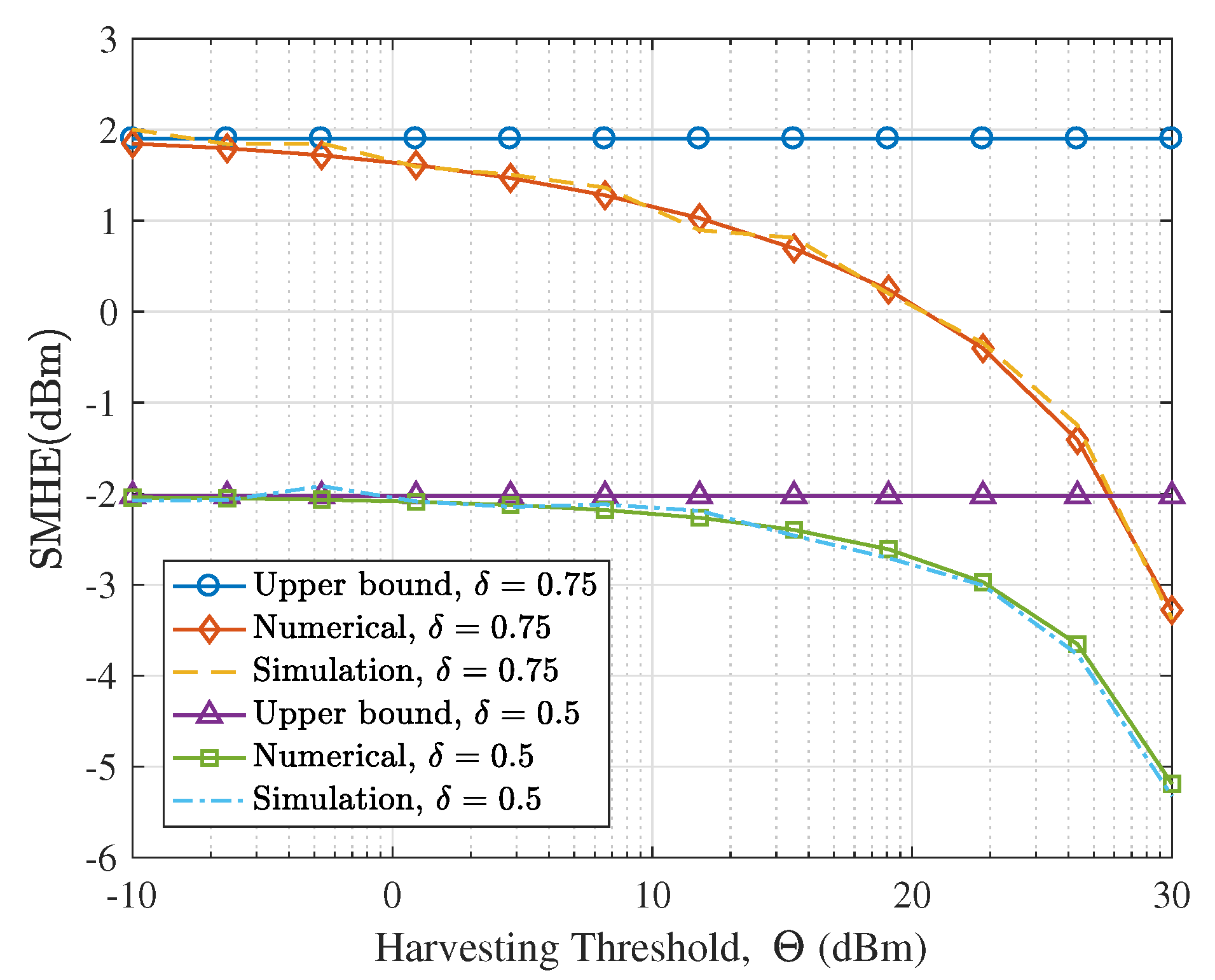
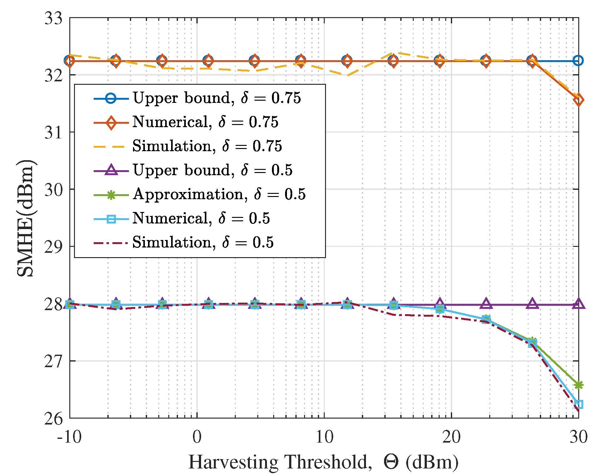
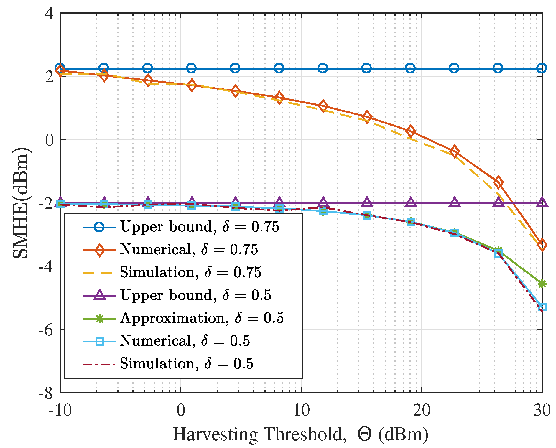
The SMHE curves of LSWN-IC with density are presented in Figure 6 and with density in Figure 7. The figures show that the simulation once again agrees with the numerical results well validating our proposed analysis framework. We also verify the numerical and the approximated results for LSWN-noIC by Monte Carlo simulations (with density and ) in Figure 8 and Figure 9. We draw two main conclusions from the above results: First, in regime of interest, i.e., below 10 dBm, the harvesting threshold has a negligible effect on the SMHE for networks with and without interference control. Second, the SMHE of LSWN-noIC is obviously larger than that of LSWN-IC for a dense network. However, their differences become less significant for a sparse network. This implies that the concurrent transmitters in a sparse network will not introduce perceptible RF energy increase on average.
5.2. Availability Analysis of Ambient RF Energy
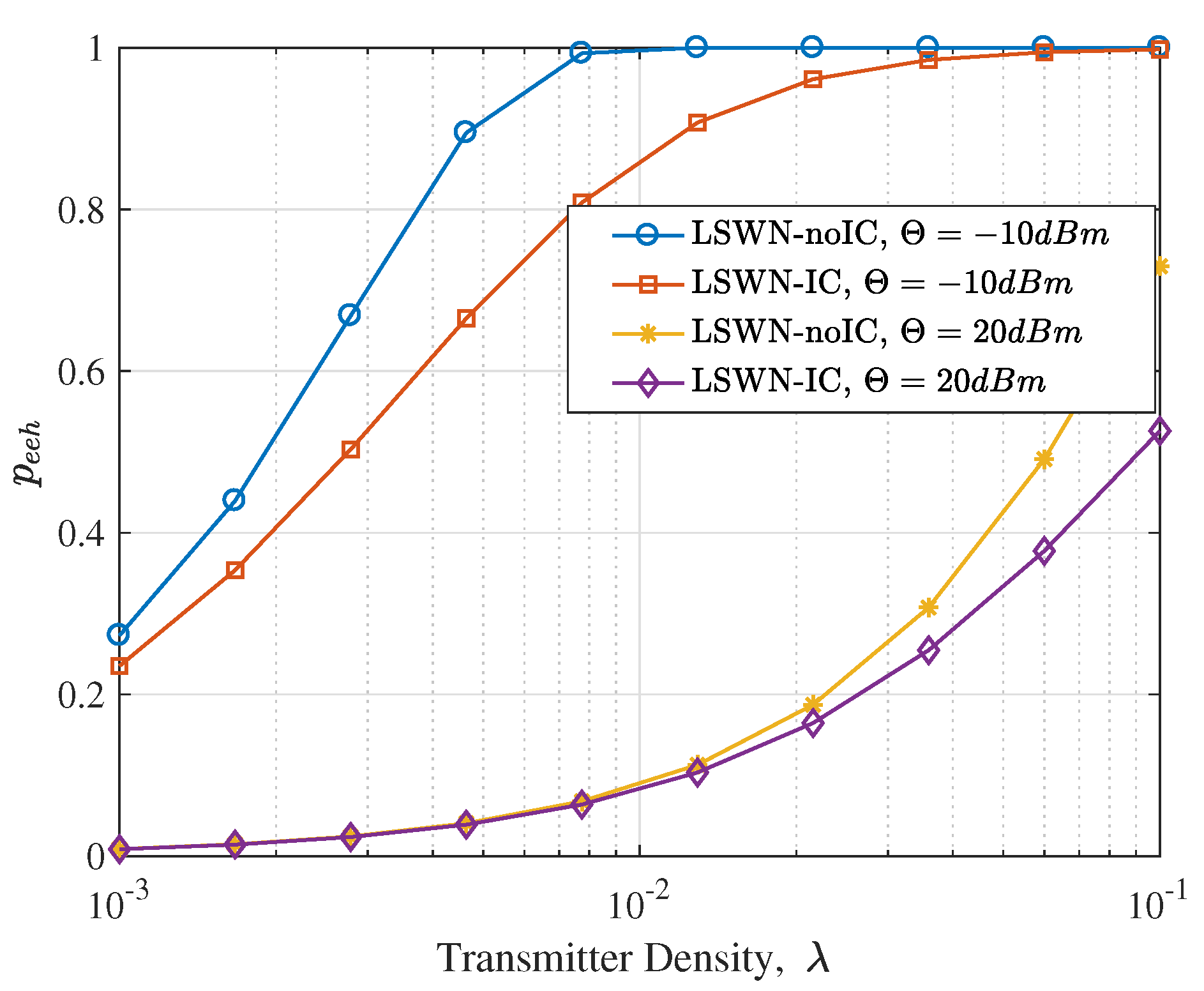
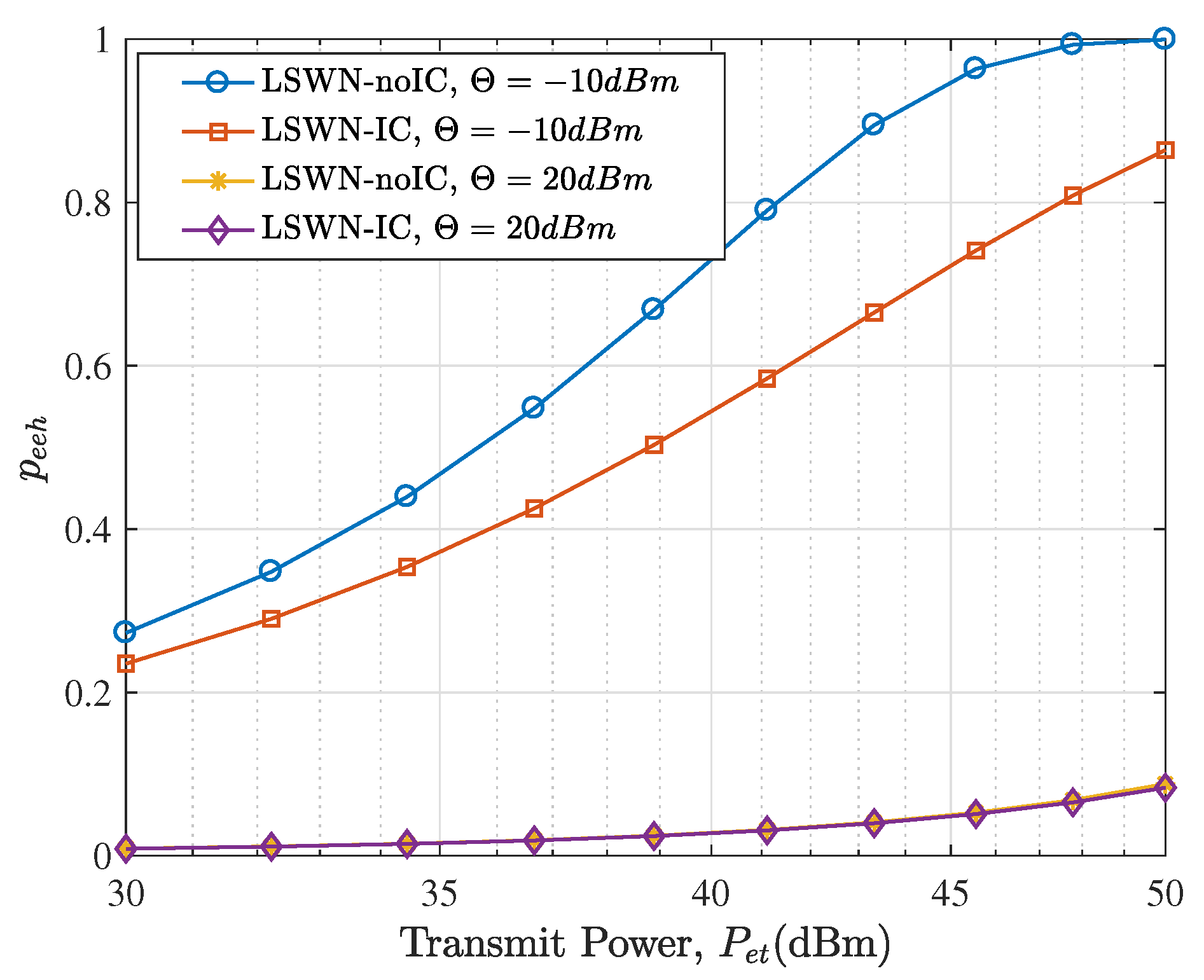
Having verified the proposed analysis framework, we now examine how EEHP and SMHE are affected by varying transmitter density and transmit power, with both protocols: LSWN-IC and LSWN-noIC. In Figure 10, we depict the EEHP for the receiver with harvesting thresholds e.g., −10 dBm and 20 dBm representing a typical sensitive and insensitive RF energy harvester, respectively. It can be seen that increasing density can dramatically improve the EEHP for both harvesting thresholds. It is worth noting that for a lower harvesting threshold, the performance gap between two protocols is larger than for a higher harvesting threshold. A similar trend is observed for EEHP versus transmit power curve as shown in Figure 11. In fact, there is almost no difference for LSWN with and without IC for a higher threshold. From this experiment we draw the following insights: harvesters with higher sensitivity can benefit more from dense networks or high-power transmitters, indicating that designing the circuit with low harvesting threshold is critical for improving the availability of ambient RF energy.
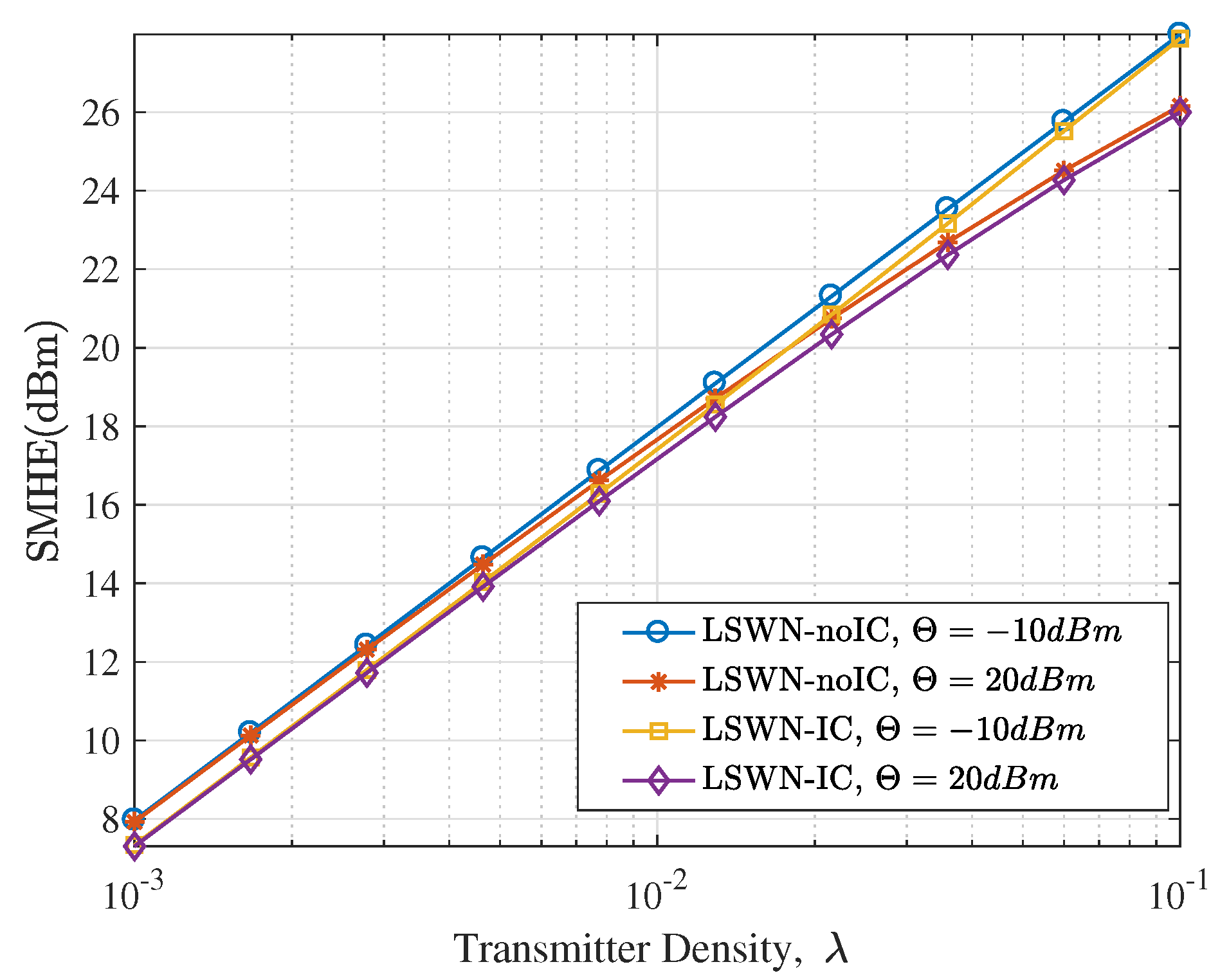
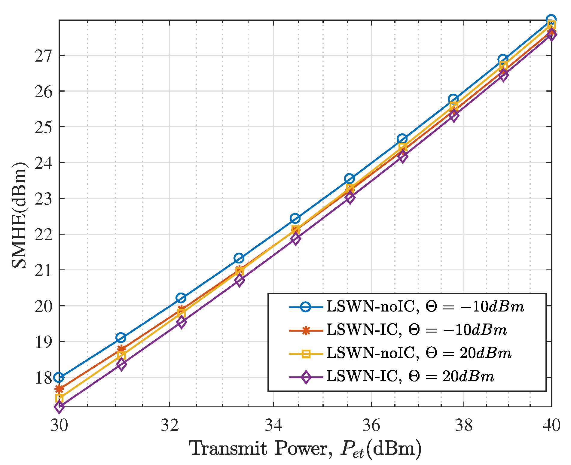
In Figure 12 and Figure 13, the relationship between SMHE and transmitter density and transmit power are presented, respectively. The main observation is that the impact of harvesting threshold on SMHE is negligible. For our simulation setup, since only a small fraction of the transmitters contribute energy less than the harvesting threshold, changes in the threshold value minimally impacts the overall harvested energy. Besides, we find that interference control has limited influence on SMHE for varying transmitter density or transmit power. However, after examining Figure 12, we find that increasing transmitter density narrows the performance gap between LSWN-IC and LSWN-noIC for same harvesting threshold. The difference in SMHE between networks with and without IC is almost a constant with increasing transmit power, as shown in Figure 13. That is to say, increasing density will bring more availability of ambient RF energy than increasing transmit power with respect to SMHE. This is consistent with the interference analysis in [38] which states that quadratic increase of transmit power is equivalent to linear increase of transmitter density from an interference perspective.
6. Conclusions
This paper has examined the availability of ambient RF energy harvested in d-dimensional large scale networks with/without interference control. The availability has been captured via two metrics namely the effective energy harvesting probability and the spatial mean harvestable energy. In contrast to previous efforts, we have considered both a bounded path loss model and impact of the energy harvesting threshold on harvesting performance. The mean and distribution of the ambient RF energy are presented exactly or approximately. For the special case of dimension to path loss ratio equal to 0.5, closed-form results are derived. Our unified framework is general and therefore the results can be applied to 1-D, 2-D, and 3-D networks. For multiple network models, the EEHP and SMHE performance are verified via simulations. We observe that the sensitivity of RF energy harvester has a significant impact on EEHP of a typical receiver. Alternately, the effect of harvesting threshold on SMHE is negligible, particularly in dense networks. Also, we point out that increasing transmitter density can enhance RF energy availability more efficiently than improving transmit power. Finally, we argue that for a sparse network, interference control has little influence on energy harvesting performance. In a further study, we plan to employ the derived results to optimize the information transfer in ambient RF energy powered networks.
Acknowledgments
The work was supported by Educational Commission of Hubei Province of China (D20162702), in part by the National Key Research and Development Program of China (2016YFB1200202), the National Natural Science Foundation of China (61771365), the Natural Science Foundation of Shaanxi Province (2017JZ022), and by the 111 Project (B08038).
Author Contributions
Hongxing Xia and Yongzhao Li conceived the manuscript idea and designed the experiments; Hongxing Xia performed the experiments; Hongxing Xia, Yongzhao Li, Hailin Zhang and Balasubramaniam Natarajan wrote and revised the paper.
Conflicts of Interest
The authors declare no conflict of interest.
References
- Mekikis, P.V.; Kartsakli, E.; Antonopoulos, A.; Alonso, L.; Verikoukis, C. Connectivity Analysis in Clustered Wireless Sensor Networks Powered by Solar Energy. IEEE Trans. Wireless Commun. 2018, PP, 1. [Google Scholar] [CrossRef]
- Bi, S.; Ho, C.K.; Zhang, R. Wireless powered communication: Opportunities and challenges. IEEE Commun. Mag. 2015, 53, 117–125. [Google Scholar] [CrossRef]
- Huang, K.; Zhong, C.; Zhu, G. Some new research trends in wirelessly powered communications. IEEE Wirel. Commun. 2016, 23, 19–27. [Google Scholar] [CrossRef]
- Lee, S.; Zhang, R.; Huang, K. Opportunistic wireless energy harvesting in cognitive radio networks. IEEE Trans. Wirel. Commun. 2013, 12, 4788–4799. [Google Scholar] [CrossRef]
- Krikidis, I. Simultaneous information and energy transfer in large-scale networks with/without relaying. IEEE Trans. Commun. 2014, 62, 900–912. [Google Scholar] [CrossRef]
- Xia, H.; Natarajan, B.; Liu, C. Feasibility of simultaneous information and energy transfer in LTE-A small cell networks. In Proceedings of the 2014 IEEE 11th Consumer Communications and Networking Conference (CCNC), Las Vegas, NV, USA, 10–13 January 2014; pp. 20–25. [Google Scholar]
- Che, Y.L.; Duan, L.; Zhang, R. Spatial Throughput Maximization of Wireless Powered Communication Networks. IEEE J. Sel. Areas Commun. 2015, 33, 1534–1548. [Google Scholar] [CrossRef]
- Mekikis, P.V.; Lalos, A.S.; Antonopoulos, A.; Alonso, L.; Verikoukis, C. Wireless Energy Harvesting in Two-Way Network Coded Cooperative Communications: A Stochastic Approach for Large Scale Networks. IEEE Commun. Lett. 2014, 18, 1011–1014. [Google Scholar] [CrossRef]
- Inaltekin, H.; Wicker, S.B. The behavior of unbounded path-loss models and the effect of singularity on computed network interference. In Proceedings of the 4th Annual IEEE Communications Society Conference on Sensor, Mesh and Ad Hoc Communications and Networks (SECON’07), San Diego, CA, USA, 18–21 June 2007; pp. 431–440. [Google Scholar]
- Zhang, R.; Ho, C.K. MIMO Broadcasting for Simultaneous Wireless Information and Power Transfer. IEEE Trans. Wirel. Commun. 2013, 12, 1989–2001. [Google Scholar] [CrossRef]
- Flint, I.; Lu, X.; Privault, N.; Niyato, D.; Wang, P. Performance analysis of ambient RF energy harvesting: A stochastic geometry approach. In Proceedings of the 2014 IEEE Global Communications Conference, Austin, TX, USA, 8–12 December 2014; pp. 1448–1453. [Google Scholar]
- Sakr, A.H.; Hossain, E. Analysis of K-Tier Uplink Cellular Networks With Ambient RF Energy Harvesting. IEEE J. Sel. Areas Commun. 2015, 33, 2226–2238. [Google Scholar] [CrossRef]
- Oliveira, D.; Oliveira, R. Modeling energy availability in RF Energy Harvesting Networks. In Proceedings of the 2016 International Symposium on Wireless Communication Systems (ISWCS), Poznań, Poland, 20–23 September 2016; pp. 383–387. [Google Scholar]
- Wang, L.; Wong, K.K.; Heath, R.W.; Yuan, J. Wireless Powered Dense Cellular Networks: How Many Small Cells Do We Need? IEEE J. Sel. Areas Commun. 2017, 35, 2010–2024. [Google Scholar] [CrossRef]
- Khan, T.A.; Heath, R.W. Wireless Power Transfer in Millimeter Wave Tactical Networks. IEEE Signal Process. Lett. 2017, 24, 1284–1287. [Google Scholar] [CrossRef]
- Zewde, T.A.; Gursoy, M.C. Energy efficiency analysis for wireless-powered cellular networks. In Proceedings of the 2017 51st Annual Conference on Information Sciences and Systems (CISS), Baltimore, MD, USA, 22–24 March 2017; pp. 1–6. [Google Scholar]
- Ma, X.; Zhang, J.; Yin, X.; Trivedi, K.S. Design and Analysis of a Robust Broadcast Scheme for VANET Safety-Related Services. IEEE Trans. Veh. Technol. 2012, 61, 46–61. [Google Scholar] [CrossRef]
- Guo, J.; Zhang, Y.; Chen, X.; Yousefi, S.; Guo, C.; Wang, Y. Spatial Stochastic Vehicle Traffic Modeling for VANETs. IEEE Trans. Intell. Transp. Syst. 2018, 19, 416–425. [Google Scholar] [CrossRef]
- Gupta, P.; Kumar, P.R. Internets in the sky: Capacity of 3D wireless networks. In Proceedings of the 39th IEEE Conference on Decision and Control, Sydney, Australia, 12–15 Decemver 2000; Volume 3, pp. 2290–2295. [Google Scholar]
- Ng, S.C.; Mao, G.; Anderson, B.D. Critical density for connectivity in 2D and 3D wireless multi-hop networks. IEEE Tran. Wirel. Commun. 2013, 12, 1512–1523. [Google Scholar] [CrossRef]
- Omri, A.; Hasna, M.O. Modeling and Performance Analysis of 3-D Heterogeneous Networks With Interference Management. IEEE Commun. Lett. 2017, 21, 1787–1790. [Google Scholar] [CrossRef]
- Zander, J. Distributed cochannel interference control in cellular radio systems. IEEE Trans. Veh. Technol. 1992, 41, 305–311. [Google Scholar] [CrossRef]
- Chiu, S.N.; Stoyan, D.; Kendall, W.S.; Mecke, J. Stochastic Geometry and Its Applications; John Wiley & Sons, Ltd: Chichester, UK, 2013. [Google Scholar]
- Andrews, J.G.; Baccelli, F.; Ganti, R.K. A Tractable Approach to Coverage and Rate in Cellular Networks. IEEE Trans. Commun. 2011, 59, 3122–3134. [Google Scholar] [CrossRef]
- Rappaport, T.S. Wireless Communications: Principles and Practice, 2nd ed.; Pearson Education: Delhi, India, 2010. [Google Scholar]
- Haenggi, M.; Ganti, R.K. Interference in Large Wireless Networks; Now Publishers Inc.: Breda, The Netherlands, 2009. [Google Scholar]
- Abeywickrama, S.; Samarasinghe, T.; Ho, C.K.; Yuen, C. Wireless Energy Beamforming Using Received Signal Strength Indicator Feedback. IEEE Trans. Signal Process. 2018, 66, 224–235. [Google Scholar] [CrossRef]
- Valenta, C.R.; Durgin, G.D. Harvesting wireless power: Survey of energy-harvester conversion efficiency in far-field, wireless power transfer systems. IEEE Microw. Mag. 2014, 15, 108–120. [Google Scholar]
- Nintanavongsa, P.; Muncuk, U.; Lewis, D.R.; Chowdhury, K.R. Design optimization and implementation for RF energy harvesting circuits. IEEE J. Emerg. Sel. Top. Circuits Syst. 2012, 2, 24–33. [Google Scholar] [CrossRef]
- Haenggi, M. On distances in uniformly random networks. IEEE Trans. Inf. Theory 2005, 51, 3584–3586. [Google Scholar] [CrossRef]
- Gradshteyn, I.S.; Ryzhik, I.M. Table of Integrals, Series, and Products (Seventh Edition). Table Integrals 2007, 103, 1161–1171. [Google Scholar]
- Lowen, S.B.; Teich, M.C. Power-law shot noise. IEEE Trans. Inf. Theory 1990, 36, 1302–1318. [Google Scholar] [CrossRef]
- Srinivasa, S.; Haenggi, M. Modeling interference in finite uniformly random networks. In Proceedings of the International Workshop on Information Theory for Sensor Networks (WITS’07), Santa Fe, NM, USA, 16–21 June 2007; pp. 1–12. [Google Scholar]
- Feller, W. An Introduction to Probability Theory and Its Applications; Wiley: New York, NY, USA, 1968; Volume 2, pp. 435–436. [Google Scholar]
- Abate, J.; Whitt, W. A unified framework for numerically inverting Laplace transforms. INFORMS J. Comput. 2006, 18, 408–421. [Google Scholar] [CrossRef]
- Kamel, M.; Hamouda, W.; Youssef, A. Ultra-Dense Networks: A Survey. IEEE Commun. Surv. Tutor. 2016, 18, 2522–2545. [Google Scholar] [CrossRef]
- Lu, W.; Di Renzo, M. Stochastic Geometry Modeling of Cellular Networks: Analysis, Simulation and Experimental Validation. In Proceedings of the 18th ACM International Conference on Modeling, Analysis and Simulation of Wireless and Mobile Systems (MSWiM’15), Cancun, Mexico, 2–6 November 2015; ACM: New York, NY, USA, 2015; pp. 179–188. [Google Scholar]
- Haenggi, M. Stochastic Geometry for Wireless Networks; Cambridge University Press: New York, NY, USA, 2012. [Google Scholar]
Figure 1.
Spatial model of d-dimensional networks for .

Figure 2.
Effective energy earvesting probability for LSWN-IC with , , and = 30 dBm.

Figure 3.
Effective energy harvesting probability for LSWN-IC with , , and = 30 dBm.

Figure 4.
Effective energy harvesting probability for LSWN-noIC with , , and = 30 dBm.

Figure 5.
Effective energy harvesting probability for LSWN-noIC with , , and = 30 dBm.

Figure 6.
Spatial mean harvestable energy for LSWN-IC with , , and = 30 dBm.

Figure 7.
Spatial mean harvestable energy for LSWN-IC with , , and = 30 dBm.

Figure 8.
Spatial mean harvestable energy for LSWN-noIC with , , and = 30 dBm.

Figure 9.
Spatial mean harvestable energy for LSWN-noIC with , , and = 30 dBm.

Figure 10.
Effective energy harvesting probability versus transmitter density with , and = 30 dBm.

Figure 11.
Effective energy harvesting probability versus transmitting power with , and .

Figure 12.
Spatial mean harvestable energy versus transmitter density with , and = 30 dBm.

Figure 13.
Spatial mean harvestable energy versus transmitter density with , and .


Table 1.
Comparison of related works.
| Literature | Network Model | Large Scale Fading Model | Small Scale Fading Model | RF Energy Harvesting Performance |
|---|---|---|---|---|
| Flint et al. [11] | Ginibre -DPP in | BPL | Not considered | Exact mean; Upper bound for CCDF |
| Sakr and Hossain [12] | K-tier HPPP in | UBPL | Rayleigh | CDF in integration form; closed-form for |
| Oliveira and Oliveira [13] | finite HPPP in | BPL | Rayleigh | Approximated CDF in infinite series, modeled by generalized Gamma distribution and Normal distribution |
| Wang et al. [14] | 2-tier HPPP in | Sub-6GHz: UBPL/ mmWave:Blockage path loss model | Sub-6GHz: Nakagami; /mmWave: not considered | sub-6GHz:CDF in integral form; exact form for infinite antennas number/ mmWave: CDF in integral form |
| Khan and Heath [15] | HPPP in | BPL | Nakagami | CDF in integral of Gamma function |
| Zewde and Gursoy [16] | HPPP in | BPL | Rayleigh | Mean in closed-form |
| Our work | HPPP in | BPL | Rayleigh | LSWN-IC: CDF in integral form; closed-form for . Mean in integral form; exact upper bound / LSWN-noIC: CDF in inverse Laplace function; lower bound for . Mean in inverse Laplace function; exact upper bound and compact approximation for . |
Table 2.
Main results.
| Network Type | EEHP | SMHE |
|---|---|---|
| LSWN-IC | Integral form in (18), exact form in (19) for | Integral form in (20); Upper bound in (24) |
| LSWN-noIC | ILT of (35); Compact upper bound in (40) for | Compound expression of ILT in (46); Upper bound in (54) and accurate approximation in (55) for |
Table 3.
Simulation parameters.
| Density | ||
|---|---|---|
| = 0.1 | L = 1000, N = | L = 200, N = |
| = 0.0001 | L = 1000, N = | L = 400, N = |
© 2018 by the authors. Licensee MDPI, Basel, Switzerland. This article is an open access article distributed under the terms and conditions of the Creative Commons Attribution (CC BY) license (http://creativecommons.org/licenses/by/4.0/).
Share and Cite
MDPI and ACS Style
Xia, H.; Li, Y.; Zhang, H.; Natarajan, B. Availability of Ambient RF Energy in d-Dimensional Wireless Networks. Energies 2018, 11, 668. https://doi.org/10.3390/en11030668
AMA Style
Xia H, Li Y, Zhang H, Natarajan B. Availability of Ambient RF Energy in d-Dimensional Wireless Networks. Energies. 2018; 11(3):668. https://doi.org/10.3390/en11030668
Chicago/Turabian StyleXia, Hongxing, Yongzhao Li, Hailin Zhang, and Balasubramaniam Natarajan. 2018. "Availability of Ambient RF Energy in d-Dimensional Wireless Networks" Energies 11, no. 3: 668. https://doi.org/10.3390/en11030668
Note that from the first issue of 2016, this journal uses article numbers instead of page numbers. See further details here.