Multi-Model Prediction for Demand Forecast in Water Distribution Networks


1
CONACYT—Consorcio CENTROMET, Camino a Los Olvera 44, Los Olvera, Corregidora, Querétaro 76904, Mexico
2
Institut de Robótica i Informática Industrial (CSIC-UPC), Carrer LLorens Artigas 4-6, Barcelona 08028, Spain
3
División de Estudios de Posgrado e Investigación, Instituto Tecnológico de Culiacán, Juan de Dios Bátiz 310 pte, Culiacán 80220, Mexico
4
División de Estudios de Posgrado de la Facultad de Ingeniería Eléctrica, Universidad Michoacana de San Nicolás de Hidalgo, Gral. Francisco J. Múgica S/N, Morelia 58040, Mexico
*
Author to whom correspondence should be addressed.
†
These authors contributed equally to this work.
Energies 2018, 11(3), 660; https://doi.org/10.3390/en11030660
Submission received: 24 February 2018
/
Revised: 11 March 2018
/
Accepted: 13 March 2018
/
Published: 15 March 2018
(This article belongs to the Special Issue Smart Water Networks in Urban Environments)
Abstract
:This paper presents a multi-model predictor called Qualitative Multi-Model Predictor Plus (QMMP+) for demand forecast in water distribution networks. QMMP+ is based on the decomposition of the quantitative and qualitative information of the time-series. The quantitative component (i.e., the daily consumption prediction) is forecasted and the pattern mode estimated using a Nearest Neighbor (NN) classifier and a Calendar. The patterns are updated via a simple Moving Average scheme. The NN classifier and the Calendar are executed simultaneously every period and the most suited model for prediction is selected using a probabilistic approach. The proposed solution for water demand forecast is compared against Radial Basis Function Artificial Neural Networks (RBF-ANN), the statistical Autoregressive Integrated Moving Average (ARIMA), and Double Seasonal Holt-Winters (DSHW) approaches, providing the best results when applied to real demand of the Barcelona Water Distribution Network. QMMP+ has demonstrated that the special modelling treatment of water consumption patterns improves the forecasting accuracy.
1. Introduction
Water is one of the most important natural resources to sustain life and to guarantee people’s quality of life. In urban areas, complex drinking water distribution network systems provide water supply from the water reservoirs to the population. The main reservoirs are conformed by lakes, rivers, and sea water, among other sources. Water transportation implies energy cost and water availability, subject to population growth and water shortage. Important objectives in water delivery through drinking water networks are the supply of the water demanded by the consumers, the reduction of operational costs related to production and transportation [1], and the maximization of the water delivery service satisfaction, among others.
Related Work
The optimal operation of drinking water networks is a critical issue for sustainable human activity. New paradigms are being used for optimizing the use of this valuable resource such as Model Predictive Control (MPC). MPC is used for optimizing water management with the aim of minimizing the water production costs and the energy required to transport the liquid from the sources to the consumers [2,3]. In general, the performance of control approaches is affected by the model quality of the real system and the forecast accuracy, such as discussed in [4] where the prediction of the hot water consumption in residential houses is used to optimize the operation of distributed water heaters. In particular, MPC for water management is affected by the model quality of the water network, the accuracy of the demand forecasting models, and the length of the prediction horizon. MPC is able to manage efficiently a water network by using a dynamical system to determine the best sequence of actions for a desired time horizon to optimize the operational objectives. From this sequence, only the first control action is applied and then the optimization process is repeated regularly, updating the water network initial conditions with the new observations.
In order to build the prediction models, the drinking water demand is studied as a time series. A time series is defined as a sequence of chronologically ordered observations recorded at regular time intervals. Those observations might correspond to qualitative or quantitative data. The motivation of this paper is to build a model that exploits the particular characteristics of the water demand consumption to produce accurate 24-h ahead forecasts.
We assume that the water consumption volume is recorded hourly using flowmeters. Time series present a cyclic consumption pattern, where each cycle repeats every 24 h. Observing those daily patterns, we detected different dynamic pattern behaviors that might be seen as the change of different regimes that need to be mathematically defined and validated. For example, in the work of [5] and Lopez Farias et al. [6], water demand usually presents different pattern behaviors in holidays and in working days, but regularly during those periods. This fact motivates the use of several models to characterize each regime.
This work is mainly related to the research carried out to identify different behaviors (regimes or modes) in time series (or dynamical systems producing such data) by means of qualitative information defined by the type of the daily drinking water demand pattern.
Regarding the multi-model time series prediction approach, we find in the state-of-the-art that the identification of regimes is a common strategy to predict information that involves human activity such as sales, electricity, and water demand.
A set of algorithms related to drinking water demand forecasting using clustering can be found in Quevedo et al. [7], where the implementation of a daily Autoregressive Integrated Moving Average (ARIMA) model combined with hourly patterns is proposed with the objective of allowing prediction at daily and hourly scales every 24 h. The ARIMA model predicts the total day consumption while a daily pattern is selected according to a calendar for distributing the hourly consumption along the day. Rodriguez Rangel et al. [8] used the concept of daily patterns (modes) predicted with the non-parametric Nearest Neighbor Mode Estimation (NNME) proposed in Lopez Farias et al. [6]. NNME is used as a regression method to forecast the modes that feeds the input of an ensemble of 24 independent artificial neural network (ANN) models trained with Genetic Algorithms; each of the ANN predicts a specific hour of the day. Nevertheless, this approach is computationally costly when the training set is big. A similar approach proposed by Candelieri [9], suggests the use of several pools (each pool associated with a type of the day) with 24 Support Vector Machines Models, each one to predict a specific hour of the day. In contrast to Rodriguez Rangel et al. [8], Candelieri’s method only classifies the current day to select the pool. Donkor et al. [10] report the use of different methodologies to improve the water demand prediction in the short term (from several hours to several days ahead) and the long term (one year or more ahead); nevertheless, it does not propose the use of regimes. Other statistical and machine learning modeling methodologies that deal with the water demand forecasting problem are found in [7,11,12,13,14]. The work of Cutore et al. [15] implement similar ideas about regimes associated with working and holy days to predict one day ahead water demand of daily time series using an ANN. The ANN architecture uses three input neurons to receive the current water demand, and its associated working or weekend day. The hidden layer also has three neurons and the output layer just one neuron that returns the predicted water consumption. This ANN model parameters are optimized with a Shuffled Complex Evolution Metropolis, a kind of evolutionary algorithm that combines Bayesian Inference and probabilistic criterion to accept or reject a set of ANN parameters.
Regarding the selection of the inputs, Romano and Kapelan [16] use a sliding window of past demand data, the day of the week, and the hour associated with the forecast horizon. The day of the week and the hour are used to associate the water demand time series to human pattern behaviours. We also found works where those human patterns are incorporated to the forecast methodology (e.g., the work of Quevedo et al. [5]), but each approach differs in the way they are incorporated. In our previous works [5,17], we have started exploring the use of a calendar (days of the week, in terms of labor days and holy days), but we found that the Qualitative Multi-Model Predictor method (QMMP) proposed in [6] improves the calendar method for certain district metering areas (DMAs).
The QMMP decomposes a raw time series in qualitative and quantitative components. The quantitative component is the daily water demand sequence, and it is predicted with a Seasonal Autoregressive Integrated Moving Average (SARIMA) model. The qualitative component has the sequence of consumption patterns and they are predicted with a model based on Nearest Neighbors (NN) identified in this paper as Nearest Neighbors Mode Estimator (NNME).
Adaptive predictive methods are also found in the literature, e.g., the algorithm proposed by Bakker et al. [18], which considers just the last two days for predicting the water demand of the next two days. The contribution of the days is weighted and a complementary fixed calendar is considered as an additional information input. After tuning the day weights, it derives day factors and demand patterns that consider daily/weakly behaviours. Martinez Alvarez et al. [19] use clustering to group days with similar patterns.
The work of Alvisi and Franchini [20] presents a probabilistic approach to assess the predictive uncertainty of water demand using a Model Conditional Processor (MCP). The MCP provides a joint probability distribution to perform a correct prediction from one or multiple predictive models using historical data, and allows the possibility of combining different forecasts with the aim of maximizing the probability of producing the most likely prediction. In their work, they use an ANN, and a simple autoregressive forecast models (AR(1)) at daily and hourly time scales. Although part of their work is similar to the one presented in this paper in the sense that multiple models are used to generate a prediction, our method focuses on dealing with the best probabilistic selection of a set of discrete prediction models, associated with categorical water demand regimes. In addition, we also deal with the adaptability considering that regimes are changing gradually.
As we mentioned before, multi-modeling is not just limited to water demand prediction; it is also used to model and predict other kinds of time series that involve human activity. Melgoza et al. [21] proposed a method for predicting electrical demand based on multiple models; each model describes a region of behavior of the system (driven by the human activity), called the operation regime. Martinez-Alvarez et al. [22] suggested the use of clustering to group similar patterns regarding the variation of the electricity cost in working and holy days. Kumar and Patel [23] and Dai et al. [24] propose a clustering-based predictive algorithm to improve sales forecasts. The data clustering is used for regime identification and training local models that combined produce the final forecast model.
The main contribution of this paper regarding the Qualitative Multi-Model Predictor (QMMP) introduced in [6] is the use of a model that probabilistically selects from three qualitative prediction models improving 24-h ahead forecast accuracy. This is achieved by choosing the most likely qualitative model to predict correctly the water distribution pattern given the hour of the day; we also propose adapting the water distribution patterns according to recent pattern variations; we call this approach Qualitative Multi-Model Predictor Plus (QMMP+).
The case study considered in this paper to show the effectiveness of the proposed approach is based on real demand from the Barcelona drinking water network. The water demand is predicted with the proposed approach and then compared with well established prediction approaches as Double Seasonal Holt-Winters (DSHW), originally proposed by C.C. Holt in 1957 and P. Winters in 1960 [25], the ARIMA, proposed the first time in 1970 by G. E. P. Box and G. M. Jenkins [26], Radial Basis Function Neural Networks (RBF-ANN) [27], and the Naïve model that just considers the recent observations as prediction.
The rest of the paper is organized as follows: Section 2 introduces the QMMP+ architecture, the decomposition of the time series into qualitative and quantitative information, the different qualitative and quantitative predictor models that perform the prediction such as: the NNME, Calendar, online Nearest Neighbor Rule Pattern Estimation (NNRPE), a Moving Average pattern update method, and a probabilistic method to select the best prediction model from this set. The Seasonal ARIMA is addressed as the quantitative model predictor. This section also presents the implementation of the training, tuning, and forecasting of our method. Section 3 presents the comparison of the experiments and results of QMMP+ against other known methods. Finally, Section 4 draws the conclusions.
2. Methods
This section describes the QMMP+ architecture and the implementation details of its Qualitative and Quantitative predictors. Finally, the tuning, training and forecasting algorithms unifying all the forecasting models to produce the final prediction are introduced.
2.1. QMMP+ Architecture
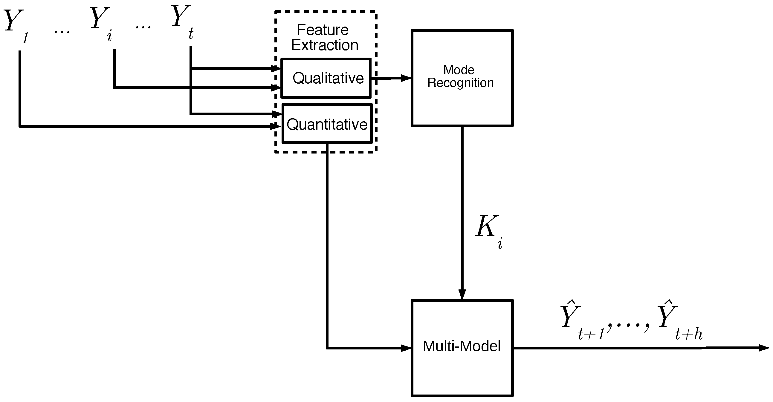
QMMP+ has the general architecture presented in Figure 1, which describes the general process of forecasting using time series decomposition. First, the raw time series is processed by the Feature Extraction to obtain the water demand time series decomposition. The demand patterns are given to the Mode Recognition to produce a pattern forecast. The Multi-Model module uses the pattern selected by the Mode Recognition and combined with the quantitative forecast produces the final forecast .
QMMP+ implements several models and algorithms to exploit the characteristics of the data responding to working, holidays and other kinds of events. A SARIMA model is used to predict the (quantitative) cumulative daily water demand and a set of three forecasting models to predict the qualitative information or consumption patterns. Qualitative forecasting models are probabilistically selected to predict the water consumption pattern of the predicted day. Two pattern mode forecasting models can be used: a Calendar-based pattern mode predictor contains a list of defined workdays and holidays. Given the day, the calendar indicates the consumption pattern during the day. This is a binary selector that assumes that working days and holidays have different consumption patterns. The second pattern predictor is based on NN; given the history of qualitative patterns, it exploits the information provided by the historical sequence of pattern modes to predict the following one. Another model works as a pattern observer each time t (hourly) to correct the pattern mode if the predicted pattern is incorrect. This observer is called Nearest Neighbor Rule Pattern Estimator (NNRPE).
2.2. Qualitative-Quantitative Time Series Decomposition
QMMP+ works with cyclic time series. A time series is a sequence defined by
where n is the total number of elements and t is the time index, representing a magnitude recorded through time. Two cumulative quantitative and qualitative time series, and , are extracted from the original time series . The new time series has elements indexed by the time index , is the accumulation period length (e.g., a day), where is the floor function used to consider complete periods. It is important to note that, for the water demand application, lowercase index and size symbols (t and n) are associated with hourly time series and the uppercase symbols (T and N) are associated with daily time series along the paper. Following this notation, the quantitative time series is obtained as follows:
where is the daily cumulative water consumption time series of each period T. The qualitative time series is produced extracting normalized vectors used as daily patterns of each period T according to
used to characterize the operating regime of period . The operating regimes are divided into classes in the set . Each is associated with one of those classes. Therefore, the sequence of categorical data representing the classes of daily patterns is defined as
where each element is a label that identifies a class or mode from , as a result of classifying each according to the most similar pattern using the function. The construction of is as follows
where , and is the set of patterns. Each is the representative pattern prototype of those vectors classified into the class .
2.3. Qualitative Predictor
This subsection addresses the description of the different qualitative prediction models: the NNME, Calendar, Nearest Neighbor Rule Pattern Estimation (NNRPE), and the probabilistic Selection of Qualitative Models that integrates the models. The aim is to produce the best prediction of the labels for the next H days, , which combined with the prediction of quantitative information , allow us to obtain the final vector prediction in an hourly basis defined as,
where is the pattern estimation set to . Similarly, the real hourly information, (in our application, water consumption) is defined by
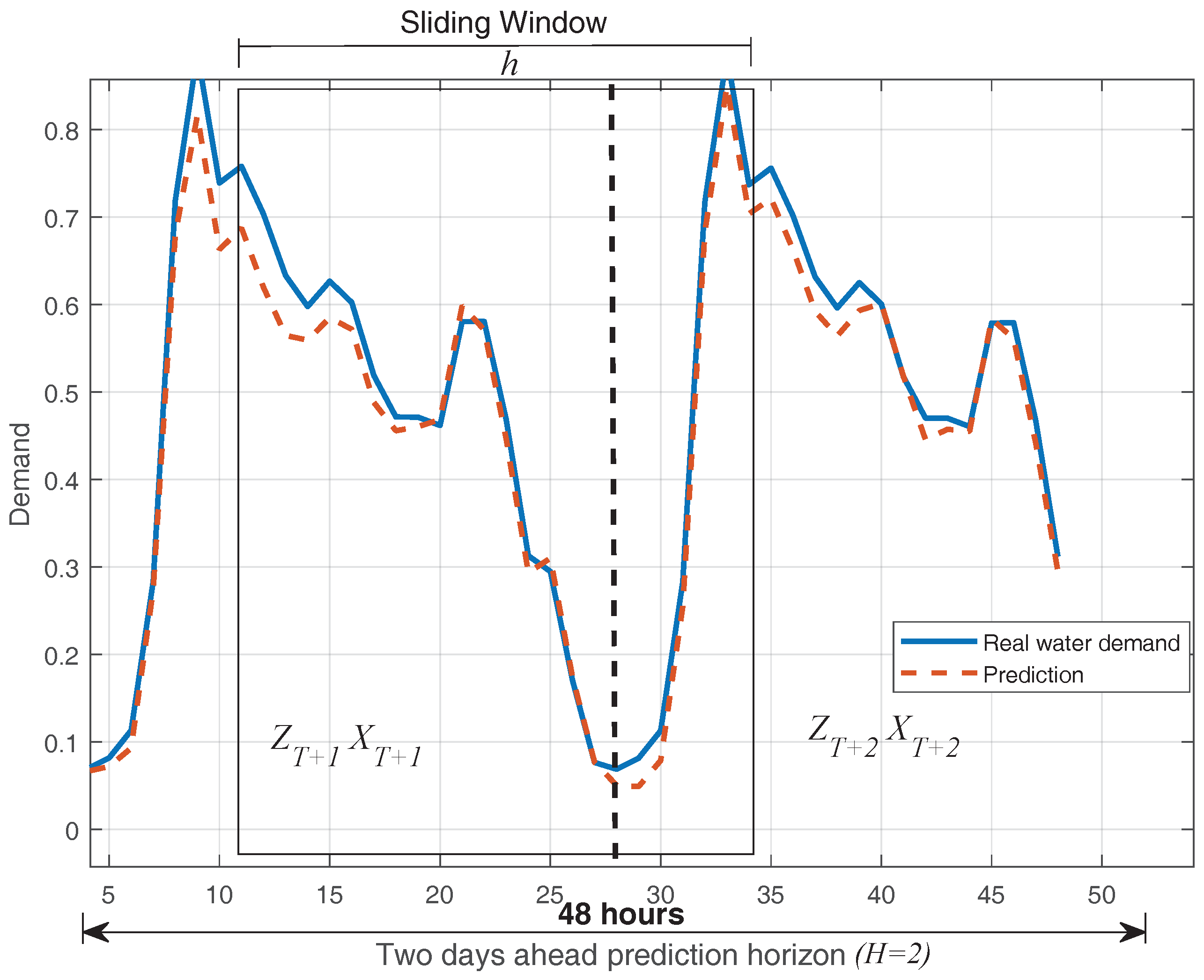
As discussed in the introduction, the application of QMMP+ to the operational MPC control of water distribution networks, it is necessary to produce 24-h ahead predictions every hour. In order to do this, two days () of water demand are estimated. The forecast in this horizon is given by , and then, to perform the hourly prediction, a sliding window of width h is used, covering the subsequence of data from to in steps as shown in Figure 2.
2.3.1. Nearest Neighbors Mode Estimator
Nearest Neighbors (NN) is an non-parametric learning algorithm that makes decisions based on the set or a subset of the training data set. This algorithm has been used for nonlinear time series prediction by Kantz and Schreiber [28]. NN assumes that the data is in a feature metric space. The considered data might be scalars, multidimensional vectors, labels, or characters. The NNME is used to solve the problem of estimating the next H categorical elements given a sequence of observed labels in . In order to implement NNME, a time series is organized in subsequences named delay vectors of the form
where (following Kantz´s notation) we use the size parameter m of the delay vector and the embedding dimension parameter fixed to 1 along the paper; therefore, it is not explicitly written in the following equations. The parameter defines the neighborhood radius size from that includes the delay vectors . Each delay vector is constructed similarly as Equation (8) by setting that satisfies
where can be any distance function. For scalars or real numbers, it is common to use the Euclidean distance, but, for comparing sequences of qualitative information, it is suitable to use the Hamming distance, defined by
where and are label vectors; the distance between vectors x and y is defined by
With the qualitative time series , we estimate the next H modes using the nearest neighbors function defined by
where receives the recent vector as an argument and it is set to using Equation (8). represents time index increments generating the next class labels sequence of size H from to of each . The forecast is produced using the statistical Mode for each next element set (e.g., next value is computed with ).
Setting , the optimization of Equation (12) is performed by means of an exhaustive search, bounding the search space and minimizing the mode prediction errors in Hamming distance using the real observations
2.3.2. Calendar
Human activity might be related and ruled by policies and traditions defined in a yearly calendar. The information given by the calendar is potentially useful for making accurate predictions. In order to integrate the calendar information to the forecasting model, we defined a function that receives the daily time T as the argument and returns the next H modes , considering a two class calendar that considers working and weekend/holiday days. Therefore, the calendar function is defined as
where the returning values depend on the coded information in the label vector and each calendar element takes values from the two class set .
2.3.3. Nearest Neighbor Rule Pattern Estimation
The Nearest Neighbor Rule Pattern Estimation (NNRPE) is a simple online approach implemented to recognize and correct the current mode in an hourly basis. Since the pattern mode is predicted every time steps with the Calendar and NNME methods, it is possible to estimate incorrectly a mode due to model inaccuracies or eventualities (e.g., unexpected pattern mode produced by a contingency plan) and therefore to use the wrong estimation pattern for the remaining period of time . This fact is solved observing the evolution of the distribution pattern along the period (i.e., day) and determining the most similar pattern with the information acquired so far. As soon as we get more information about the current day pattern, the mode estimation will tend to be the same as the real pattern mode. In order to compare the current observed data with the available pattern modes, the recent data is normalized considering past measurements to make the data comparable with the patterns with
Once the last measurements are normalized, we proceed to choose the most similar pattern so far with the comparison function
where provides the hour of the day associated with using the module function, , which is the time index fixed to the first hour of the current day. These indexes make it possible to compare the pattern to the current normalized observations using vectors of same length. Figure 3 presents an example. Let us assume that we are at time instant . If , then the hour of the day is 13 (). Therefore, we compare the first 13 pattern elements of each with the last 13 elements of the normalized vector (elements inside the dashed square).
Figure 4 shows the distance of within the dashed square of Figure 3. The pattern evolution from hours 1 to 5 is apparently closer to ; nevertheless, the trend is inverted from hour 6, switching the estimation to pattern , which generates the minimum distance with the data so far. The closeness of is estimated via nearest neighbor and the correction is presented when the similarity index changes. In this way, the estimation will be more accurate as we observe more data.
2.3.4. Probabilistic Selection of Qualitative Models
The probabilistic selection of Qualitative Models is performed by computing the probability of each qualitative predictor to produce the best pattern prediction using past data. For the case , we select the model from the predictor set composed by , , , with the highest probability to predict better than others in a specific hour of the day . For the case of predicting , similarly, we select the model from the predictor set composed by and . The Selection of Qualitative Model for predicting is stored in and is expressed as the model that maximizes the probability of predicting correctly
where has the independent probabilities of each predictor model to have the best estimation in the past, given the hour of the day denoted by . , , are the same functions defined in Equations (14), (16), and (12), with the difference that we consider the prediction at a specific hour of the day.
The probabilities of each model F to predict given the hour of the day are computed considering the total of correct predictions divided by the sum of correct and incorrect predictions. This is computed as
where is the number of times when F has predicted historically correct, which is at hour , and otherwise. The same approach is used to predict , with the difference that neither nor the hour are considered. The probability is computed as
As discussed in [17], the pattern distribution models are changing gradually over time. Thus, once we have the mechanism to predict the qualitative behavior, we propose to extend the model using an adaptive mechanism based on a simple Moving Average (MA) to update the distribution modes. In order to do this, the most recent patterns associated with and are collected in sequence as follows:
Finally, the distribution pattern to be used for the prediction is updated by producing an average of the last patterns associated with the predicted mode
where is a positive integer indicating the number of the last patterns used to produce an update of , given by the average of the last patterns . Then, the obtained distribution pattern is considered as the new pattern to be used in the prediction.
2.4. Seasonal ARIMA as Quantitative Predictor
ARIMA is a statistical regression methodology, which assumes the existence of linear temporal relations among the elements of the time series [26]. ARIMA can be seen as a time series dynamical model where the future estimations are explained with the current and past available data. Seasonal ARIMA (SARIMA) is the generalization for the time series with a seasonal pattern. This model uses four polynomials expressed by SARIMA , where p and q define the polynomial degree of each AR and MA component and d is the difference order of the integrated non-seasonal component. Similarly to the seasonal component, P and Q define the polynomial degree of each seasonal AR and MA component, respectively, and D is the number of seasonal differences every lags for the seasonal integrated part.
As an example, a SARIMA model produces the model expressed with lag operators,
where L is the lag operator that returns the previous element of a time series (e.g., ), d and D are the integration order set to 1 for the seasonal and non-seasonal component, and are the polynomial coefficients for non-seasonal and seasonal AR, and and are the coefficients for the non-seasonal and seasonal MA considering the first seasonal difference lag at time 7. is the non-seasonal difference, and is the seasonal differences every seven steps.
2.5. QMMP+ Implementation
This section describes the details of the QMMP+ implementation, integrating the different elements described in the previous subsections, in both training and operational phases. The training and forecasting algorithms assume that the time series (1) has been transformed into qualitative and quantitative time series with the format introduced in Equations (2) and (3), respectively. The formatted time series is represented by
Then, the available data is divided into training and testing sets. The training set is composed by a subset of elements defined by in the training set; the remaining corresponds to the validation set. Using this set, we tune and learn the different parameters of the algorithms. The training process is presented in detail in Algorithms 1 and 2, in the next subsection. The full forecasting process is presented in Algorithm 3 in the operational phase subsection.
| Algorithm 1 Tuning Parameters |
| Algorithm 2 Optimize Moving Average Parameter |
|
| Algorithm 3 Forecasting |
2.5.1. Training Phase
The training phase is summarized in Algorithm 1, which takes as arguments the training sets of the qualitative and quantitative time series . In line 2, a subset size is set in order to evaluate parameters using time series data from to . In line 3, we find the SARIMA model for that performs the Ljung–Box test via autocorrelation analysis. In line 4, we learn the prototypes from the qualitative TS using k-means; those prototypes are stored in vector . Then, a clustering with k classes is selected that produces the maximum separability according to the Silhouette Coefficient proposed by [29]. In line 5, the prototypes are used as input for the full data qualitative patterns classification, producing the sequence of labels assigned to vector by using Equation (5). The loop from lines 6 to 8 produces the sets containing all the patterns associated with a prototype, line 9 optimizes NN qualitative forecasting model selecting the delay vector size m and neighborhood size according to Equation (13). Line 10 optimizes the number of the last qualitative patterns for the adaptive pattern MA.
The function is presented in Algorithm 2. It tests the different values from to , keeping the value that produces the least prediction error for the k classes.
2.5.2. Operational Phase
In the operational phase, the multi-model predictor architecture presented in Figure 1 is implemented. The model receives the raw measurements every hour as input to be converted every steps in qualitative patterns, using the Qualitative Feature Extraction module and aggregated data by using the Quantitative Feature Extraction module (model of Figure 1). The classification labels are provided to the Mode Detection module to estimate the next pattern using , and , and then used by the Multi-Model Forecasting module.
The operational phase procedure describes how the forecast is performed. The process is described in Algorithm 3, which returns all the 24-h horizon forecasts each hour inside the vector . The prediction is performed with unknown data in the time interval from to . Lines 3 and 4 produce two qualitative predictions with NNME and the Calendar. In line 5, SARIMA produces the next two quantitive values. Line 6 saves the Calendar and NNME predictions in their respective label estimation arrays (e.g., ) with using Equations (18) and (19).
Then, from lines 7 to 18, the prediction is performed at each step every cycle. Line 9 normalizes the last measurements and saves them in vector . Line 10 updates the patterns using Equation (21). Line 11 computes the time to be used in line 12. Line 12 estimates the current pattern with NR rule defined in Equation (16). Line 13 stores the estimation in associated with the . Line 14 produces the most likely Pattern Prediction for given by . Line 15 similarly produces the most likely Pattern Prediction for given by . Line 16 is used to produce the final prediction h steps ahead. Line 16 saves the water demand prediction for the 24 h ahead. Line 19 saves the real pattern and line 20 updates the occurrences with the real patterns, and the probabilities associated with each qualitative predictor, and, finally, line 22 returns the predictions produced every hour.
3. Results and Discussion
This section presents the application of the QMMP+ to forecast the water demand of the Barcelona drinking water network and the obtained performance results.
Application and Study Case
The water demand from the Barcelona drinking water network is used as a case study in this paper. This network is managed by Aguas de Barcelona SA (AGBAR), which supplies drinking water to Barcelona and its metropolitan area. The main water sources are the rivers Ter and Llobregat.
Figure 5 shows the general topology of the network, which has 88 main water consumption sectors. Currently, there are four water treatment plants: the Abrera and Sant Joan Despí plants, which extract water from the Llobregat river; the Cardedeu plant, which extracts water from the Ter river; and the Besòs plant, which treats underground water from the Besòs river aquifer. There are also several underground sources (wells) that can provide water through pumping.
This network has 4645/km of pipes supplying water from sources to serve 23 municipalities within an extension of 424 km, satisfying the water demand of 3 million people approximately, providing a total flow around of 7 m/s.
For the MPC control, a prediction horizon of 24 h is sufficient to operate with a good balance in accuracy and performance. MPC also operates hourly and is fed with the current and estimated water demand for 24 h ahead by a forecasting model. The QMMP+ approach is used to provide 24-h ahead water demand forecast.
For assessing the performance of the proposed approach, hourly time series are generated by representative flowmeter measurements of the year 2012 (from a total of 88) of the Barcelona network. The selection criterion is to consider only complete time series with regular data and few outliers according to the modified Thomson Tau () method. The part of its name is given by the statistical expression ), where t is the Student’s value and n the total number of elements.
The time series associated with different urban areas sectors, are identified with alphanumeric codes in the water demand database: p10007, p10015, p10017, p10026, p10095, p10109 and p10025. According to the Thomson Tau test, with a significance of , these sectors contain less than 70 outliers with exception of Sector p10025, which has an irregular data segment producing more outliers. Briefly, the Thomson Tau test detects the potential outlier using the Student’s t-test, labeling the data as outlier when its distance is larger than two standard deviations from the mean.
We enumerate the selected sensor sectors using new labels from 1 to 7, respectively, to simplify the legend in the table of results. All the time series are normalized in the [0,1] interval. The forecast accuracy of the QMMP+ is measured and compared with well-known forecasting models such as ARIMA [26], where the ARIMA structures are estimated with R’s autoarima function. The structure coefficients are optimized using MATLAB´s estimate function (Matlab R2017a, MathWorks Inc., Natick, MA, USA), and the test is also implemented in MATLAB with the forecast function. The Double Seasonal Holt Winters (DSHW) [25], available in the R forecast package, implemented the dshw function to fit the model. The RBF Neural Networks [27], available in the MATLAB Neural Network Toolbox package, implemented the function to learn the neural network’s weights. MATLAB is also used to implement k-means and silhouette coefficient to identify the qualitative patterns.
All methods are tuned and trained using a training set with of data. The remaining data is used as validation set to measure the performance accuracy 24 steps or hours ahead using the Mean Absolute Error (), Root Mean Squared Errors () and Mean Absolute Percentage Error () defined as,
where n is the size of the training set, h is the forecasting horizon and , is the first element of the validation set.
We also report precision with the variance of all the independent forecasting residuals stored in a vector of size equal to the number of individual forecasts (given by multiplying the number of forecasts by the horizon h), , where each residual is defined as the difference of the real and forecasted values defined as follows:
The index j is the result of mapping the prediction time indexes at all different times and horizons to the vector defined as,
Once we have , the variance of the individual residuals is computed by
where E is the statistical expectation.
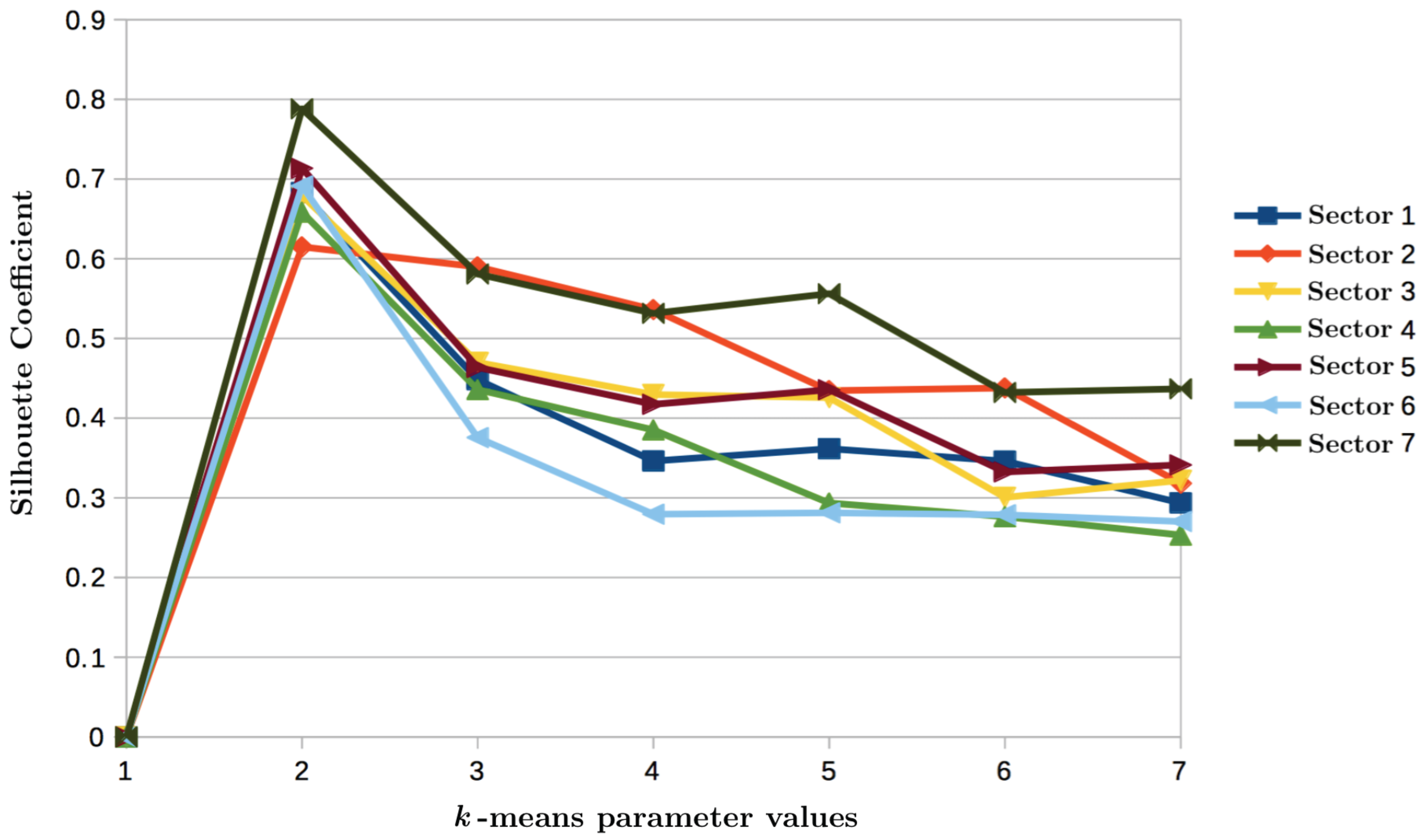
The distribution patterns are clustered using k-means. Each distribution (or class) is represented by the normalized centroid . The number of classes is defined by maximizing the silhuette coefficient. To achieve this, k-means is executed testing different number of classes k from 2 to 7. The silhouette coefficient for each time series is reported in Figure 6, which indicates that a value of maximizes the separability of the qualitative patterns for the studied time series. The centroids obtained with k-means represent the average pattern of each pattern demand class used as initial mode or prototypes.
The training set is used to learn the NNME parameters associated with the function, and the validation set measures its performance with different values of and m. We optimize Equation (13) for and .
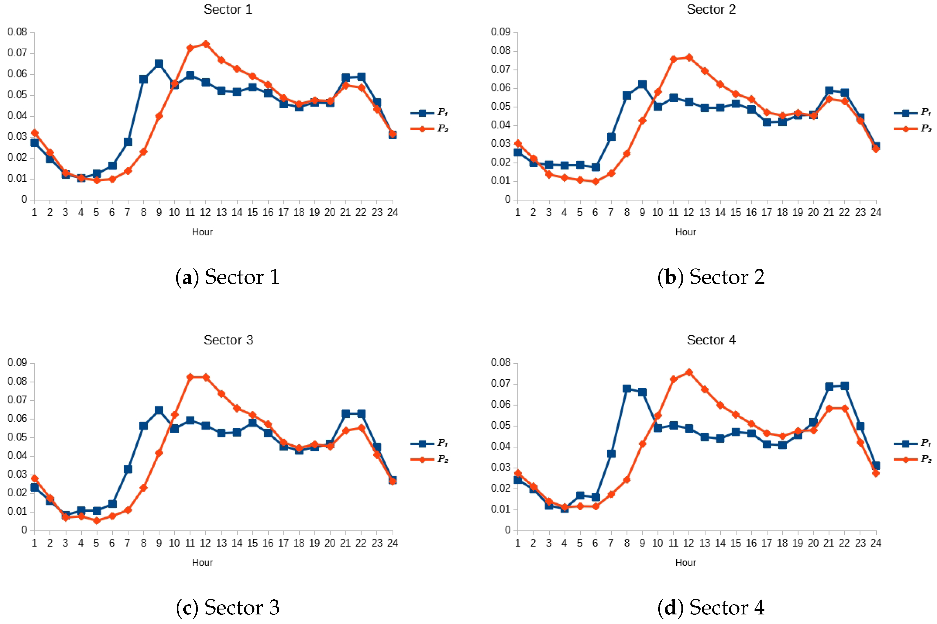
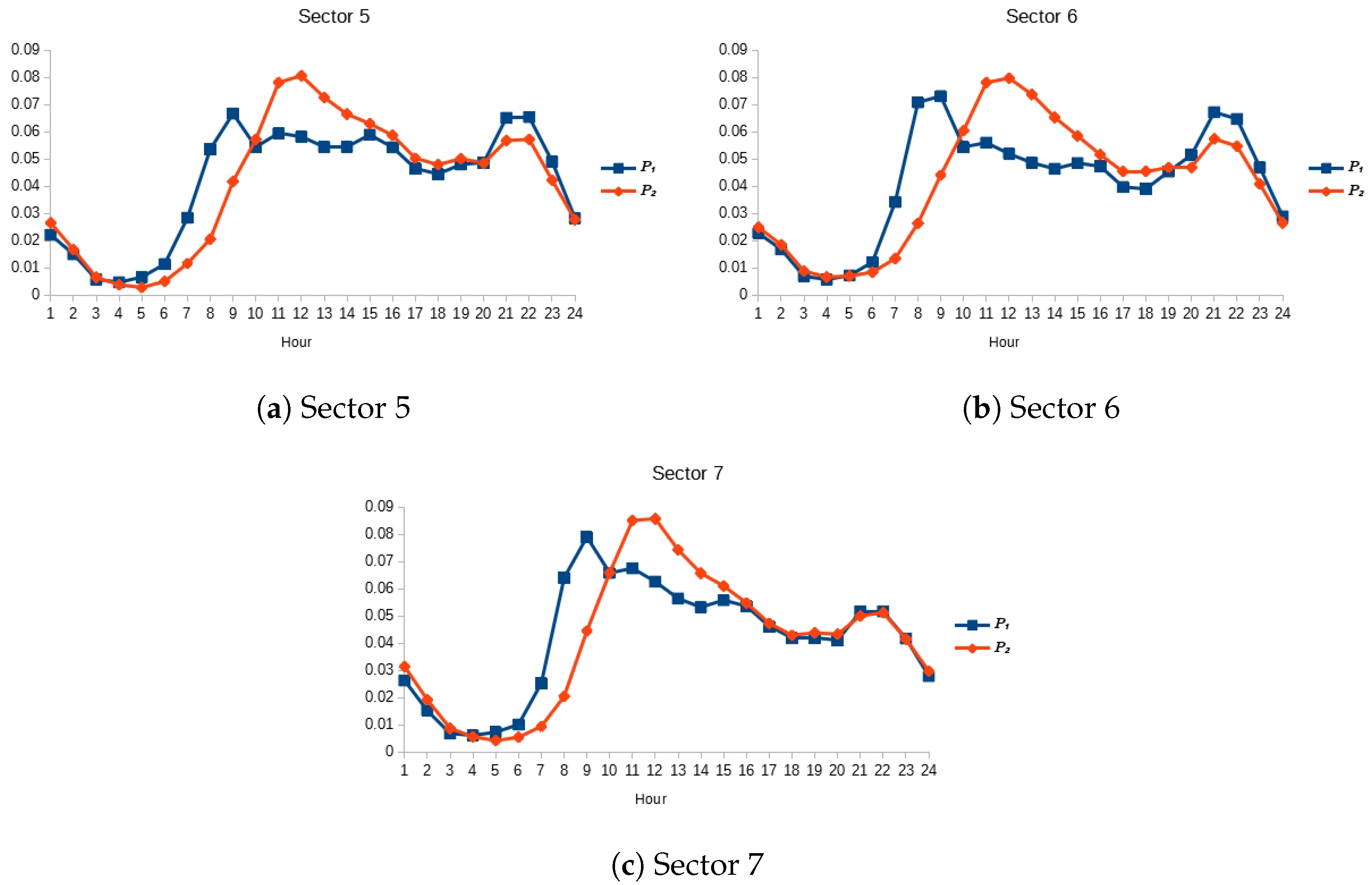
For the MA adaptive pattern, we test the lag values . Table 1 presents the SARIMA structures and the specific polynomial lags associated with each component of the model. Each model passed the Ljung–Box test once they are optimized. Table 1 also reports the best m and for NNME, and the best lag for MA for each time series. The initial distribution of consumption patterns are presented in Figure 7 and Figure 8 , where the blue line with squares represents the holiday pattern, and the orange line with rhombi the weekday pattern.
For the calendar model, we classify the pattern in two classes associated with the 2012 Catalan calendar activity [30] (holidays and weekdays), in order to perform the mode prediction.
The QMMP+ model is compared against the DSHW, Radial Basis Function Neural Network (RBF-ANN), ARIMA and the decomposition based approaches Calendar and NNME, where NNME is the implementation of the QMMP introduced in [6]. The DSHW model has only two manually adjusted parameters indicating the seasonality; and . Since we manage hourly data, and are set to 24 and 168 for the daily and weekly periods, respectively. We present the performance obtained using the implementation in R.
In the case of the RBF-NN, the structure size is implemented using 92 Gaussian neurons in the hidden layer with , 24 inputs and 24 outputs to produce a prediction of 24 steps ahead each time step. We also include a Naïve prediction model as a reference that uses the last 24 observations to produce the forecast horizon 24 steps ahead. This model is described by
Table 2, Table 3 and Table 4 report the accuracy in terms of , and of the proposed forecasting model QMMP+ compared with the Calendar (Cal), NNME, Naïve, ARIMA, RBF-ANN (ANN) and DSHW.
Table 5 reports the prediction uncertainty for each water distribution sector, and, at the bottom of the table, the mean of the variances produced with each model.
Regarding the accuracy results, we observe that the set of decomposition based approaches, QMMP+, Calendar, and NNME, perform better in average than RBF-ANN, ARIMA and DSHW for , , and for all the water demand time time series.
In particular, ARIMA presents the less accurate predictions for all the time series, even with errors above the Naïve model. DSHW shows better results than ARIMA, and Naïve, and, finally, ANN presents the best prediction accuracy among these approaches.
Regarding the accuracy in terms of mean errors of the decomposition based approaches, (i.e., Calendar and NNME), we note two facts: on the one hand, Calendar is generally more accurate than NNME, but it requires a priori information assuming that the qualitative modes are defined by an activity calendar. On the other hand, NNME is less accurate than Calendar but able to produce good qualitative mode predictions without any assumption. This fact is useful when Calendar does not explain the sequence of modes, as the case of time series 7, where Calendar is not better than NNME. Therefore, we can say that these characteristics are complementary, and, once they are combined (as QMMP+ does), both contribute to produce more accurate forecasts.
Regarding the mean of the individual variances of Table 5, QMMP+, Calendar, and NNME are also the most precise approaches on average than Naïve, ANN, ARIMA and DSHW, where ARIMA also presents the worst precision, and only in time series 7, NNME and ANN are better than QMMP+.
In summary, we can conclude that our approach, QMMP+, outperforms the other forecasting models and shows the effectiveness of choosing probabilistically the best qualitative model throughout the experiments.
4. Conclusions
The main contribution of this paper is the introduction of the probabilistic selection of qualitative model predictors and estimators, included in the Multi-model predictor architecture called QMMP+. The model is based on the decomposition of the qualitative and quantitative information of the time-series. Seasonal ARIMA is suitable for predicting the daily consumption prediction, and NNME plus the Calendar, for mode pattern prediction. The patterns are also updated using a simple Moving Average. The NNME, Calendar and Nearest Neighbor Rule models are executed simultaneously, and then the prediction of the most suitable model is selected using a criterion based on probability. The final water demand estimation is composed of the magnitude of consumption prediction for the day and the most likely distribution pattern to appear. This QMMP+ implementation outperforms the previous QMMP reported in [6], which was also better than RBF-ANN, SARIMA, and DSHW. As future work, we propose implementing this method with another kind of time series with similar periodic behavior such as electricity demand. The probabilistic selection of qualitative prediction models allows running several prediction models and selecting in real time during the operational phase the best one according to its probability of success. We will consider the use of Bayesian networks to develop a probabilistic model selection mechanism, considering more variables to improve the accuracy of the pattern prediction.
Supplementary Materials
The code as supplementary material is found at https://github.com/rdglpz/QMMP_EXPERIMENTS.git.
Acknowledgments
This work has been partially funded by the Spanish Ministry of Economy and Competitiveness (MINECO) and the European Union through FEDER program through the projects DEOCS (ref. DPI2016-76493-C3-3-R) and HARCRICS (ref. DPI2014-58104-R).
Author Contributions
Rodrigo Lopez Farias and Vicenç Puig developed the forecasting model core and the experiments design. Hector Rodriguez Rangel, contributed with the interpretation of the results and experiment design; Juan J. Flores contributed to the interpretation and validity of the results, notation, important model design improvements and writing style. All the authors have contributed equally to the manuscript writing.
Conflicts of Interest
The authors declare no conflict of interest.
References
- De Marchis, M.; Milici, B.; Volpe, R.; Messineo, A. Energy saving in water distribution network through pump as turbine generators: Economic and environmental analysis. Energies 2016, 9, 877. [Google Scholar] [CrossRef]
- Leirens, S.; Zamora, C.; Negenborn, R.; De Schutter, B. Coordination in urban water supply networks using distributed model predictive control. In Proceedings of the 2010 IEEE American Control Conference (ACC), Baltimore, MD, USA, 30 June–2 July 2010; pp. 3957–3962. [Google Scholar]
- Ocampo-Martinez, C.; Puig, V.; Cembrano, G.; Quevedo, J. Application of predictive control strategies to the management of complex networks in the urban water cycle [applications of control]. IEEE Control Syst. 2013, 33, 15–41. [Google Scholar] [CrossRef]
- Gelažanskas, L.; Gamage, K.A.A. Forecasting hot water consumption in residential houses. Energies 2015, 8, 12702–12717. [Google Scholar] [CrossRef] [Green Version]
- Quevedo, J.; Puig, V.; Cembrano, G.; Blanch, J.; Aguilar, J.; Saporta, D.; Benito, G.; Hedo, M.; Molina, A. Validation and reconstruction of flow meter data in the Barcelona water distribution network. Control Eng. Pract. 2010, 18, 640–651. [Google Scholar] [CrossRef] [Green Version]
- Lopez Farias, R.; Puig, V.; Rodriguez Rangel, H. An implementation of a multi-model predictor based on the qualitative and quantitative decomposition of the time-series. In Proceedings of the ITISE 2015, International Work-Conference on Time Series, Granada, Spain, 1–3 July 2015; pp. 912–923. [Google Scholar]
- Quevedo, J.; Saludes, J.; Puig, V.; Blanch, J. Short-term demand forecasting for real-time operational control of the Barcelona water transport network. In Proceedings of the 2014 22nd Mediterranean Conference of Control and Automation (MED), Palermo, Italy, 16–19 June 2014; pp. 990–995. [Google Scholar]
- Rodriguez Rangel, H.; Puig, V.; Lopez Farias, R.; Flores, J.J. Short-Term Demand Forecast Using a Bank of Neural Network Models Trained Using Genetic Algorithms for the Optimal Management of Drinking Water Networks. J. Hydroinform. 2016, 1–15. [Google Scholar] [CrossRef]
- Candelieri, A. Clustering and Support Vector Regression for water demand forecasting and anomaly detection. Water 2017, 9, 224. [Google Scholar] [CrossRef]
- Donkor, E.A.; Mazzuchi, T.A.; Soyer, R.; Alan Roberson, J. Urban water demand forecasting: Review of methods and models. J. Water Resour. Plan. Manag. 2012, 140, 146–159. [Google Scholar] [CrossRef]
- Zhou, S.; McMahon, T.; Walton, A.; Lewis, J. Forecasting daily urban water demand: A case study of Melbourne. J. Hydrol. 2000, 236, 153–164. [Google Scholar] [CrossRef]
- Alvisi, S.; Franchini, M.; Marinelli, A. A short-term, pattern-based model for water-demand forecasting. J. Hydroinform. 2007, 9, 39–50. [Google Scholar] [CrossRef]
- Al-Hafid, M.S.; Al-maamary, G.H. Short term electrical load forecasting using holt-winters method. Al-Rafadain Eng. J. 2012, 20, 15–22. [Google Scholar]
- Tiwari, M.K.; Adamowski, J.F. An ensemble wavelet bootstrap machine learning approach to water demand forecasting: A case study in the city of Calgary, Canada. Urban Water J. 2017, 14, 185–201. [Google Scholar] [CrossRef]
- Cutore, P.; Campisano, A.; Kapelan, Z.; Modica, C.; Savic, D. Probabilistic prediction of urban water consumption using the SCEM-UA algorithm. Urban Water J. 2008, 5, 125–132. [Google Scholar] [CrossRef]
- Romano, M.; Kapelan, Z. Adaptive water demand forecasting for near real-time management of smart water distribution systems. Environ. Model. Softw. 2014, 60, 265–276. [Google Scholar] [CrossRef] [Green Version]
- Lopez Farias, R.; Flores, J.J.; Puig, V. Multi-model forecasting based on a qualitative and quantitative decomposition with nonlinear noise filter applied to the water demand. In Proceedings of the ROPEC 2015 (2015 IEEE International Autumn Meeting on Power, Electronics and Computing), Guerrero, Ixtapa, Mexico, 4–6 November 2015. [Google Scholar]
- Bakker, M.; Vreeburg, J.; van Schagen, K.; Rietveld, L. A fully adaptive forecasting model for short-term drinking water demand. Environ. Model. Softw. 2013, 48, 141–151. [Google Scholar] [CrossRef]
- Martinez Alvarez, F.; Troncoso, A.; Riquelme, J.; Riquelme, J. Partitioning-clustering techniques applied to the electricity price time series. In Intelligent Data Engineering and Automated Learning-IDEAL 2007; Springer: Berlin, Germany, 2007; pp. 990–999. [Google Scholar]
- Alvisi, S.; Franchini, M. Assessment of predictive uncertainty within the framework of water demand forecasting using the Model Conditional Processor (MCP). Urban Water J. 2017, 14, 1–10. [Google Scholar] [CrossRef]
- Melgoza, J.J.R.; Flores, J.J.; Sotomane, C.; Calderón, F. Extracting temporal patterns from time series data bases for prediction of electrical demand. In MICAI 2004: Advances in Artificial Intelligence; Springer: Berlin/Heidelberg, Germany, 2004; pp. 21–29. [Google Scholar]
- Martinez-Alvarez, F.; Lora, A.T.; Santos, J.C.R.; Santos, J.R. Partitioning-clustering techniques applied to the electricity price time series, IDEAL. In Lecture Notes in Computer Science; Yin, H., Tiño, P., Corchado, E., Byrne, W., Yao, X., Eds.; Springer: Cham, Switzerland, 2007; Volume 4881, pp. 990–999. [Google Scholar]
- Kumar, M.; Patel, N.R. Using clustering to improve sales forecasts in retail merchandising. Ann. OR 2010, 174, 33–46. [Google Scholar] [CrossRef]
- Dai, W.; Chuang, Y.Y.; Lu, C.J. A clustering-based sales forecasting scheme using Support Vector Regression for computer server. Procedia Manuf. 2015, 2, 82–86. [Google Scholar] [CrossRef]
- Taylor, J. Short-term electricity demand forecasting using Double Seasonal Exponential Smoothing. J. Oper. Res. Soc. 2003, 54, 799–805. [Google Scholar] [CrossRef]
- Box, G.; Jenkins, G. Time Series Analysis: Forecasting and Control, 1st ed.; Holden-Day: San Francisco, CA, USA, 1970. [Google Scholar]
- Park, J.; Sandberg, I.W. Universal approximation using radial basis-function networks. Neural Comput. 1991, 3, 246–257. [Google Scholar] [CrossRef]
- Kantz, H.; Schreiber, T. Nonlinear time series analysis, 2nd ed.; Cambridge University Press: Cambridge, UK, 2004. [Google Scholar]
- Rousseeuw, P.J. Silhouettes: A graphical aid to the interpretation and validation of cluster analysis. J. Comput. Appl. Math. 1987, 20, 53–65. [Google Scholar] [CrossRef]
- Reuters, T. Calendario Laboral de Cataluña—2012 (Working Calendar of Catalonia—2012). Available online: http://goo.gl/aMmfQX (accessed on 25 January 2018).
Figure 1.
Qualitative-quantitative multi-model architecture.

Figure 2.
Hourly prediction of water consumption using a sliding window of width h.

Figure 3.
Nearest Neighbor Rule with the current observations.
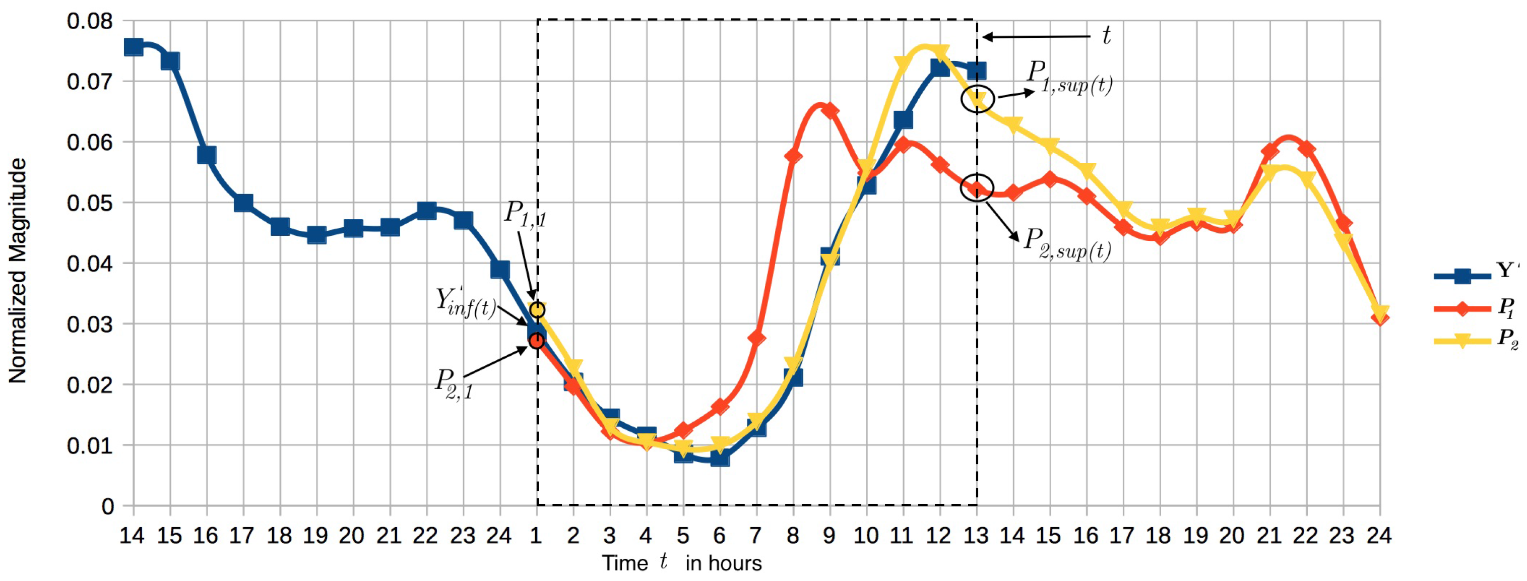
Figure 4.
Euclidean distance of along the time compared with and .

Figure 5.
Barcelona drinking water transport network.

Figure 6.
Silhouette coefficient obtained by running k-Means with different , for each of the seven water distribution sectors.
Figure 6.
Silhouette coefficient obtained by running k-Means with different , for each of the seven water distribution sectors.

Figure 7.
Initial patterns of sectors 1 to 4.

Figure 8.
Initial patterns of sectors 5 to 7.


Table 1.
Seasonal Autoregressive Integrated Moving Average (SARIMA) structures, Moving Average (MA) and Nearest Neighbor Mode Estimator (NNME) parameters for each time series.
Table 1.
Seasonal Autoregressive Integrated Moving Average (SARIMA) structures, Moving Average (MA) and Nearest Neighbor Mode Estimator (NNME) parameters for each time series.
| Sector | SARIMA Structure | MA | NNME | ||
|---|---|---|---|---|---|
| Order (p,d,q)(P,D,Q) | Polynomial Lags | m | |||
| 1 | (4,1,1)(0,0,1) | ([1,2,3,19],[1],[1])([0],[0],[7]) | 5 | 12 | 0.1 |
| 2 | (2,1,1)(0,0,1) | ([2,4],[1],[1])([0],[0],[7]) | 6 | 8 | 0.4 |
| 3 | (2,1,1)(0,0,1) | ([2,4],[1],[1])([0],[0],[7]) | 5 | 12 | 0.0 |
| 4 | (2,1,1)(0,0,1) | ([2,4],[1],[1])([0],[0],[7]) | 9 | 8 | 0.0 |
| 5 | (2,1,1)(0,0,1) | ([2,4],[1],[1])([0],[0],[7]) | 9 | 5 | 0.0 |
| 6 | (2,1,1)(0,0,1) | ([2,4],[1],[1])([0],[0],[7]) | 11 | 5 | 0.0 |
| 7 | (0,1,7)(0,0,1) | ([0],[1],[2–7])([0],[0],[5–7]) | 5 | 7 | 0.0 |
Table 2.
Mean Absolute Errors for 24 steps ahead forecasts ().
| TS | QMMP+ | Cal | NNME | Naïve | ARIMA | ANN | DSHW |
|---|---|---|---|---|---|---|---|
| 1 | 0.0261 | 0.0309 | 0.0325 | 0.0431 | 0.2268 | 0.0417 | 0.0383 |
| 2 | 0.0361 | 0.0469 | 0.0503 | 0.0556 | 0.1719 | 0.0493 | 0.0402 |
| 3 | 0.0351 | 0.0400 | 0.0436 | 0.0577 | 0.1404 | 0.0497 | 0.0500 |
| 4 | 0.0323 | 0.0346 | 0.0402 | 0.0516 | 0.1355 | 0.0437 | 0.0413 |
| 5 | 0.0336 | 0.0363 | 0.0414 | 0.0476 | 0.2226 | 0.0427 | 0.0670 |
| 6 | 0.0211 | 0.0225 | 0.0242 | 0.0286 | 0.0565 | 0.0269 | 0.0221 |
| 7 | 0.0378 | 0.0436 | 0.0388 | 0.0476 | 0.2681 | 0.0397 | 0.0568 |
| mean | 0.0317 | 0.0364 | 0.0387 | 0.0474 | 0.1745 | 0.0420 | 0.0451 |
TS: Time Series. QMMP+: Qualitative Multi-Model Predictor Plus; NNME: Nearest Neighbor Mode Estimator. DSHW: Double Seasonal Holt-Winters; ARIMA: Autoregressive Integrated Moving Average. ANN: Artificial Neural Networks.
Table 3.
Root Mean Squared Errors for 24 steps ahead forecasts ().
| TS | QMMP+ | Cal | NNME | Naïve | ARIMA | ANN | DSHW |
|---|---|---|---|---|---|---|---|
| 1 | 0.0359 | 0.0408 | 0.0435 | 0.0647 | 0.2725 | 0.0575 | 0.0506 |
| 2 | 0.0459 | 0.0608 | 0.0657 | 0.0749 | 0.2034 | 0.0626 | 0.0524 |
| 3 | 0.0472 | 0.0522 | 0.0576 | 0.0809 | 0.1740 | 0.0650 | 0.0730 |
| 4 | 0.0438 | 0.0459 | 0.0542 | 0.0719 | 0.1656 | 0.0577 | 0.0570 |
| 5 | 0.0442 | 0.0466 | 0.0543 | 0.0684 | 0.2677 | 0.0563 | 0.0996 |
| 6 | 0.0275 | 0.0291 | 0.0319 | 0.0402 | 0.0693 | 0.0353 | 0.0310 |
| 7 | 0.0508 | 0.0592 | 0.0510 | 0.0723 | 0.3141 | 0.0568 | 0.0716 |
| mean | 0.0422 | 0.0478 | 0.0512 | 0.0676 | 0.2095 | 0.0559 | 0.0622 |
Table 4.
Mean Absolute Percentage Errors for 24 steps ahead forecasts ().
| TS | QMMP+ | Cal | NNME | Naïve | ARIMA | ANN | DSHW |
|---|---|---|---|---|---|---|---|
| 1 | 7.6894 | 10.3604 | 11.0294 | 12.2260 | 104.7789 | 11.8758 | 10.9463 |
| 2 | 10.5045 | 13.9536 | 15.3083 | 16.3679 | 60.3339 | 13.8914 | 11.0999 |
| 3 | 15.1210 | 22.0860 | 23.2323 | 23.0632 | 42.3286 | 19.1763 | 69.8373 |
| 4 | 11.4644 | 13.0279 | 14.9782 | 17.6226 | 54.4792 | 15.1678 | 15.4631 |
| 5 | 15.1439 | 16.9219 | 18.7183 | 19.1025 | 934.3022 | 20.9310 | 26.9577 |
| 6 | 15.8718 | 16.5053 | 17.8853 | 21.2534 | 40.0381 | 20.4805 | 19.4827 |
| 7 | 13.2686 | 15.7276 | 14.5825 | 16.6595 | 787.0257 | 22.9499 | 19.9238 |
| mean | 12.7234 | 15.5118 | 16.5335 | 18.0422 | 289.0409 | 17.7818 | 24.8158 |
Table 5.
Mean of the individual variances.
| TS | QMMP+ | Cal | NNME | Naïve | ARIMA | ANN | DSHW |
|---|---|---|---|---|---|---|---|
| 1 | 0.0022 | 0.0024 | 0.0030 | 0.0065 | 0.0804 | 0.0040 | 0.0040 |
| 2 | 0.0028 | 0.0043 | 0.0054 | 0.0076 | 0.0467 | 0.0047 | 0.0036 |
| 3 | 0.0030 | 0.0034 | 0.0045 | 0.0088 | 0.0293 | 0.0050 | 0.0077 |
| 4 | 0.0027 | 0.0028 | 0.0042 | 0.0071 | 0.0294 | 0.0041 | 0.0053 |
| 5 | 0.0029 | 0.0031 | 0.0044 | 0.0068 | 0.0786 | 0.0047 | 0.0189 |
| 6 | 0.0010 | 0.0011 | 0.0013 | 0.0021 | 0.0050 | 0.0013 | 0.0012 |
| 7 | 0.0039 | 0.0053 | 0.0038 | 0.0081 | 0.1126 | 0.0038 | 0.0079 |
| mean | 0.0026 | 0.0032 | 0.0038 | 0.0067 | 0.0546 | 0.0040 | 0.0070 |
© 2018 by the authors. Licensee MDPI, Basel, Switzerland. This article is an open access article distributed under the terms and conditions of the Creative Commons Attribution (CC BY) license (http://creativecommons.org/licenses/by/4.0/).
Share and Cite
MDPI and ACS Style
Lopez Farias, R.; Puig, V.; Rodriguez Rangel, H.; Flores, J.J. Multi-Model Prediction for Demand Forecast in Water Distribution Networks. Energies 2018, 11, 660. https://doi.org/10.3390/en11030660
AMA Style
Lopez Farias R, Puig V, Rodriguez Rangel H, Flores JJ. Multi-Model Prediction for Demand Forecast in Water Distribution Networks. Energies. 2018; 11(3):660. https://doi.org/10.3390/en11030660
Chicago/Turabian StyleLopez Farias, Rodrigo, Vicenç Puig, Hector Rodriguez Rangel, and Juan J. Flores. 2018. "Multi-Model Prediction for Demand Forecast in Water Distribution Networks" Energies 11, no. 3: 660. https://doi.org/10.3390/en11030660
Note that from the first issue of 2016, this journal uses article numbers instead of page numbers. See further details here.