Article

Development and Validation of 3D-CFD Injection and Combustion Models for Dual Fuel Combustion in Diesel Ignited Large Gas Engines

1
Large Engines Competence Center, 8010 Graz, Austria
2
Faculty of Mechanical Engineering and Naval Architecture, University of Zagreb, 10002 Zagreb, Croatia
3
AVL List GmbH, Graz 8020, Austria
4
Institute of Internal Combustion Engine and Thermodynamics, Graz University of Technology, 8010 Graz, Austria
*
Author to whom correspondence should be addressed.
Energies 2018, 11(3), 643; https://doi.org/10.3390/en11030643
Submission received: 27 February 2018 / Revised: 9 March 2018 / Accepted: 11 March 2018 / Published: 14 March 2018

Abstract

:
This paper focuses on improving the 3D-Computational Fluid Dynamics (CFD) modeling of diesel ignited gas engines, with an emphasis on injection and combustion modeling. The challenges of modeling are stated and possible solutions are provided. A specific approach for modeling injection is proposed that improves the modeling of the ballistic region of the needle lift. Experimental results from an inert spray chamber are used for model validation. Two-stage ignition methods are described along with improvements in ignition delay modeling of the diesel ignited gas engine. The improved models are used in the Extended Coherent Flame Model with the 3 Zones approach (ECFM-3Z). The predictive capability of the models is investigated using data from single cylinder engine (SCE) tests conducted at the Large Engines Competence Center (LEC). The results are discussed and further steps for development are identified.

1. Introduction

1.1. Motivation

With the greater use of renewable energy sources (solar and wind), large engines are becoming more important for grid stabilization because of their very good transient behavior and the possibility of setting up modular systems [1]. In the transportation sector, which will triple by 2050 according to a recent study [2], large engines will also play a central role. While power generation will mainly rely upon gas engines [3], the diesel engine will still dominate the transportation (marine, rail) sector as the main source of propulsion. Accounting for 80% of transportation services worldwide, the marine sector in particular is coming under increased pressure and needs to catch up to land-based applications in terms of emission limits [4,5]. Low emission gas engines are favored as a solution to meet the very stringent emission requirements for marine applications. This requires further expansion of the gas infrastructure; in recent years a great amount of research into liquefied natural gas has been undertaken [6].
Besides standard gas and diesel combustion concepts, fully flexible dual fuel combustion concepts that can burn diesel and gas simultaneously have also become established in the large engine sector in recent years. Mobile applications such as marine or rail traction as well as stationary applications such as generator sets for power generation are available with dual fuel combustion systems [7,8,9,10]. However, today dual fuel technology is employed primarily in the marine sector as a consequence of the currently unfavorable development in the price of natural gas compared to the price of crude oil [11].
Besides producing lower emissions, dual fuel engines have a great advantage over diesel engines because they are able to generate the required power even in case of an interruption in the gas supply due to the redundancy of usable fuels. Especially in the marine sector, it is important to ensure robust and reliable ignition and combustion as well as high fuel flexibility.

1.2. Dual Fuel Technology

This paper focuses on one of these dual fuel concepts, the diesel ignited gas engine concept. It is also referred to as the diesel-gas engine, cf. [12]. The diesel ignited gas engine is operated using a homogeneous lean mixture in the combustion chamber. A small amount of diesel fuel provides the required ignition energy. It is injected into the lean mixture and starts the flame front propagation. Its application in large bore engines, which are mainly used in maritime transportation and energy production, is being researched in [13,14,15,16]. As mentioned previously, the advantages of the diesel ignited gas engine concept over the pure diesel engine are its fuel flexibility and lower NOx and soot emissions. Nevertheless, several disadvantages come hand in hand with greater fuel flexibility and have to be taken into account; these are outlined in [17]. The main disadvantage is that the efficiency is lower than with the pure gas engine. In addition, NOx emissions are higher than with a gas engine. However, the comparatively low engine-out NOx emissions are prescribed by the International Maritime Organization (IMO) Tier III [4] limit, which can be achieved by gas engines without making use of exhaust gas aftertreatment [18,19,20]. Therefore, it is critical to introduce dual fuel engines into the area of ship propulsion to meet the limits in Emission Controlled Areas (ECAs) in particular [18].

1.3. State-of-the-Art Simulation of Dual Fuel Combustion

Since the combustion principle in the diesel ignited gas engine includes more than one combustion regime, understanding the physical phenomena involved is a complex task. 3D-CFD simulation provides spatial and temporal information on the parameters for diesel ignited gas engine combustion. Besides experiments, it is therefore the most suitable tool for better understanding these phenomena. Numerical modeling of dual fuel combustion has proven to be challenging as all combustion regimes (i.e., autoignition, diffusion combustion and premixed flame front propagation) have to be modeled simultaneously. This issue can be addressed with detailed chemistry, where combustion is depicted by describing all the reactions involved in a reaction mechanism. Reduced chemical reaction mechanisms are used in 3D-CFD simulations to accurately depict the chemistry of the combustion process. The works of several authors [21,22,23,24,25] show that detailed chemistry to depict dual fuel combustion has to include all necessary reactions for both fuels used in the combustion. To describe turbulence, engine simulation with detailed chemistry is mostly limited to the Reynolds Averaged Navier Stokes (RANS) framework for engineering applications. Even with this approach to turbulence modeling, the computational time required to calculate combustion in internal combustion engines (ICE) with detailed chemistry is comparably large. Combustion models, on the other hand, can provide faster results but are usually only suitable for one type of combustion regime. A viable combination of different combustion models for autoignition and flame front propagation has been shown in [26]. An approach that can cover all regimes at the same time is the ECFM-3Z model. Developed by Colin et al. [27] and subsequently improved regarding ignition, mixing and post-oxidation phenomena [28,29,30], the ECFM-3Z is able to depict all necessary combustion regimes simultaneously. A feasible workflow with the ECFM-3Z for dual fuel combustion simulation is shown in [31], where the regime transition from autoignition to premixed flame front propagation is covered by an approach to modeling the initial flame surface density.
The present paper describes the numerical modeling of a diesel ignited gas engine using a 3D-CFD tool. The challenges of numerical simulation are identified with a special focus on the modeling of pilot injection and the interaction of the two fuels. The paper is divided into several subsections that describe the modified phases in the diesel ignited gas engine in sequence: injection, autoignition of the mixture and flame front propagation. The ECFM-3Z framework is only partly stated in this paper; cf. [11,16,32] for detailed information on the combustion model framework and mathematical background. N-heptane is used as the diesel surrogate fuel and methane as the natural gas, but the framework is not solely limited to these fuels. The influence of the fuels on ignition delay is considered by expanding the two-stage ignition delay tabulation method by an additional table dimension to include the fuel mixture fraction of both fuels. Furthermore, an interpolation function for the two-stage interpolation is introduced. An interpolation between the laminar flame speed of diesel and the laminar flame speed of natural gas is proposed to compare the flame front propagation of the two fuels. To obtain a better depiction of the diesel pilot injection, measurements of the injector were performed in a quiescent spray chamber and a Bosch Tube. The rate of injection with the diesel pilot injector was measured as well as the liquid and vapor penetration lengths, which were obtained using Schlieren and Mie scattering imaging methods [33]. The numerical and experimental results were compared and satisfactory agreement was found between the penetration lengths of the diesel masses injected. The parameter set found in these spray tests was later used in the engine simulations. The combustion modeling was then validated with engine measurements performed on a single cylinder engine at the test beds of the Large Engines Competence Center (LEC) at Graz University of Technology. The results are discussed for their validity and further ideas for model improvements are provided.

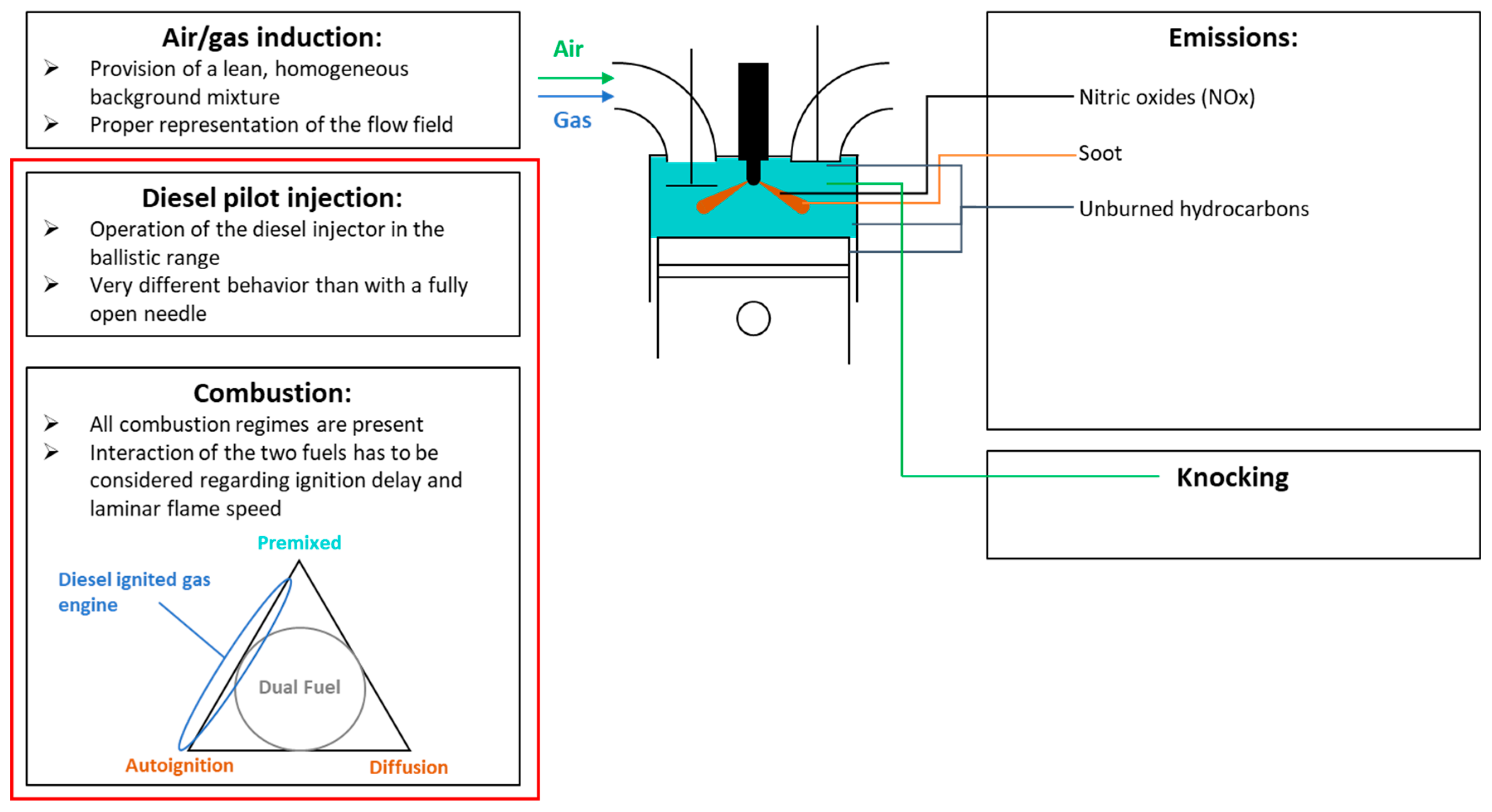
2. Challenges of Dual Fuel Combustion Modeling

Numerical simulation of a dual fuel engine has to depict several key phenomena, cf. Figure 1. The following subsection will refer to this figure as a general guideline for describing the individual challenges. Each challenge will be described along with recent research including experimental work and modeling approaches. As this paper focuses on the spatial and temporal resolution of injection, subsequent ignition and flame front propagation, a separate section is devoted to each of these challenges following this section.
The first challenge that arises is mixture preparation of the natural-gas air mixture. The air and gas induction into the cylinder has to be depicted correctly to determine the mixture fraction of this natural gas and air background mixture as well as the flow field and turbulence conditions at inlet valve closing conditions. This cold flow problem has already been thoroughly researched and described in the literature [34,35] and will not be discussed in this paper.
Diesel injection following the compression of the natural gas-air mixture is important for the ignition process. The penetration length of the diesel spray as well as its mixing with the surrounding media determines the ignition location(s), cf. [36,37]. The ignition process is also controlled by chemistry. The research in [38,39,40,41] has shown experimentally and numerically that ignition delay is dependent on the fuel mixture fraction of natural gas and diesel. The autoignition of the mixture then starts the flame front propagation throughout the lean background mixture.
The transition process between these two combustion regimes is the focus of ongoing scientific research. Based on direct numerical simulation, recent works [42,43] have identified key parameters that influence the time between autoignition and flame front propagation.
As soon as a premixed flame front has developed, the flame propagates through the homogeneous background mixture. An accurate description of the laminar flame speed is necessary to depict the heat release rate coming from flame front propagation. Once again, the laminar flame speed depends on the two fuels involved in the combustion process; with n-heptane methane mixtures, it was able to be shown experimentally [44] and numerically [41,45].
Emission modeling of nitric oxides (NOx) is possible with the NOx mechanisms currently available such as the extended Zeldovich mechanism [46]. Donateo et al. have applied this mechanism for emission prediction in dual fuel engines in their recent work [21,47]. With soot formation as well, the literature on diesel and gasoline engines provides a framework that can be used for dual fuel engine combustion simulation [35]. However, the exact process of soot formation is still not understood perfectly and therefore its prediction is greatly limited. Recent research, therefore, relies on experimental work, cf. [15]. To predict unburned hydrocarbons, which is especially important in dual fuel engines due to the methane slip, Kuppa [48] has developed a numerical model.
Another topic of active research is knocking in dual fuel engines. Knock models of gasoline and diesel engines can serve as a basis for knocking in dual fuel engines. The knocking index proposed in [49] is the numerical approach used in this paper.
Numerical research was performed using AVL FIRE (Version 2014.2) (AVL List GmbH, Graz, Austria). Focusing on injection and ignition modeling and numerical description of flame front propagation, the following subsections briefly introduce the models used and emphasize the adjustments required for dual fuel simulation. Fundamental equations of the submodels are only mentioned if needed for the dual fuel adjustments.

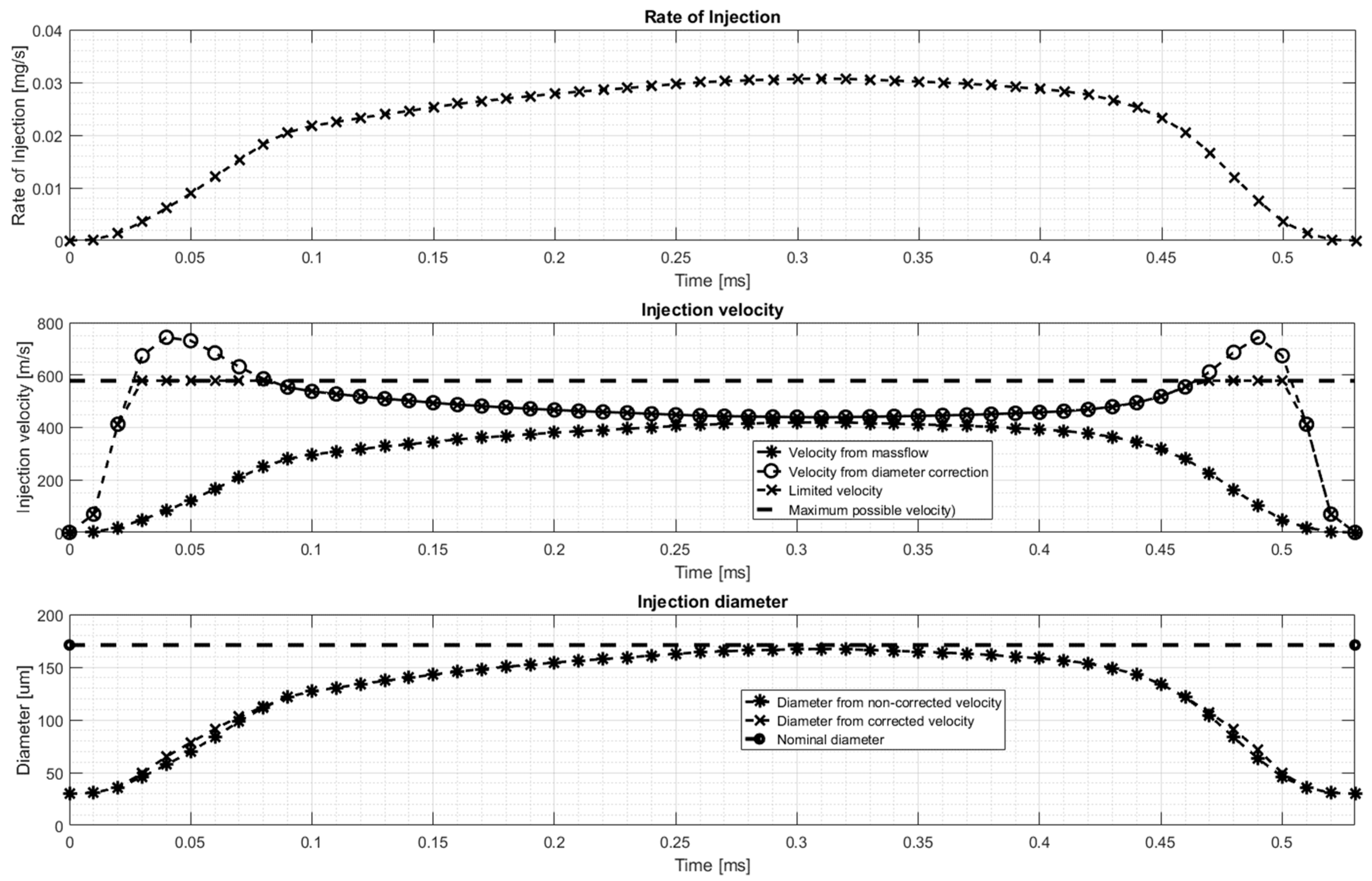
2.1. Injection Modeling

In the injection modeling process, evaporation and breakup are the two most important factors for locating the space in which the diesel spray will ignite. The WAVE child breakup model based on the work of Reitz [50] was used for the breakup process of the droplets. Further information on the software implementation can be found in [51]. The Dukowicz evaporation model was used to model the evaporation process—basic model information can be found in [52]; for its implementation, see [51].
Especially the breakup process is influenced by the location of cavitation in the nozzle hole. Various authors have demonstrated these influences with a common rail type diesel injector [35,53,54]. As there was no information available on the cavitation locations to feed the simulation model with an accurate dataset, the penetration length was calibrated by modifying the nozzle hole diameter used in the blob model [50]. Based on a simple mass flow equation for a spherical opening, Equation (1) states how the droplet velocity is calculated at the beginning of the injection:
v =   4 m ˙ ρ d 2 π
v represents the velocity of the droplets, m ˙ is the fuel mass flow, ρ describes the fuel density and d is the diameter of the nozzle hole. Since the mass flow measured equals zero at the beginning of the injection, the droplet velocity that is specified in the simulation model is also zero at the beginning. This means that the speed at which the droplets enter the simulation domain is too low. This does not have a significant impact when normal diesel engines are simulated since the needle stays open for a longer amount of time than with the diesel ignited gas engine concept, where the needle mostly operates within the ballistic region. To compensate for the problem of an inlet velocity initially too low, a non-constant nozzle hole diameter d is specified. The shape of this non-constant diameter curve follows the shape of the rate of injection (ROI), meaning the diameter is smaller at the beginning of the injection and reaches a maximum when the needle is fully open. The minimum possible diameter is a modification parameter; the maximum diameter can be calculated by Equation (2), where the maximum possible diameter d m a x is a function of the nominal nozzle hole diameter d n o m as well as drag coefficient c d and velocity coefficient c v . Values for the coefficients were estimated using the information in [35]:
d m a x =   d n o m c d c v
This leads to a significant increase in droplet velocity at the beginning of the simulation as shown in Figure 2. One can clearly see that the velocity of the droplets increases significantly when compared to the standard calculation from Equation (1). It can also happen that velocities higher than the maximum possible velocity may occur. Therefore, the diameter is corrected again to allow only for velocities lower than the one shown in Equation (3):
v m a x =   c v 2 ( p i n j p c ) ρ d i e s e l
v m a x is the maximum velocity used to limit and correct the diameter. c v is the velocity coefficient as previously shown in Equation (2). p i n j is the injection pressure, p c is the back pressure of the medium and ρ d i e s e l is the density of the diesel fuel. All of the variables were known for the injection measurements that are shown in the subsequent sections.
With this modification, the model can now consider the ballistic region of the needle lift and the resulting penetration lengths of vapor and liquid mass. Further calibration was achieved using the standard breakup and evaporation model constants as described in [51]. The results for the validation of this model approach can be found in Section 3 “Validation of injection modeling”.

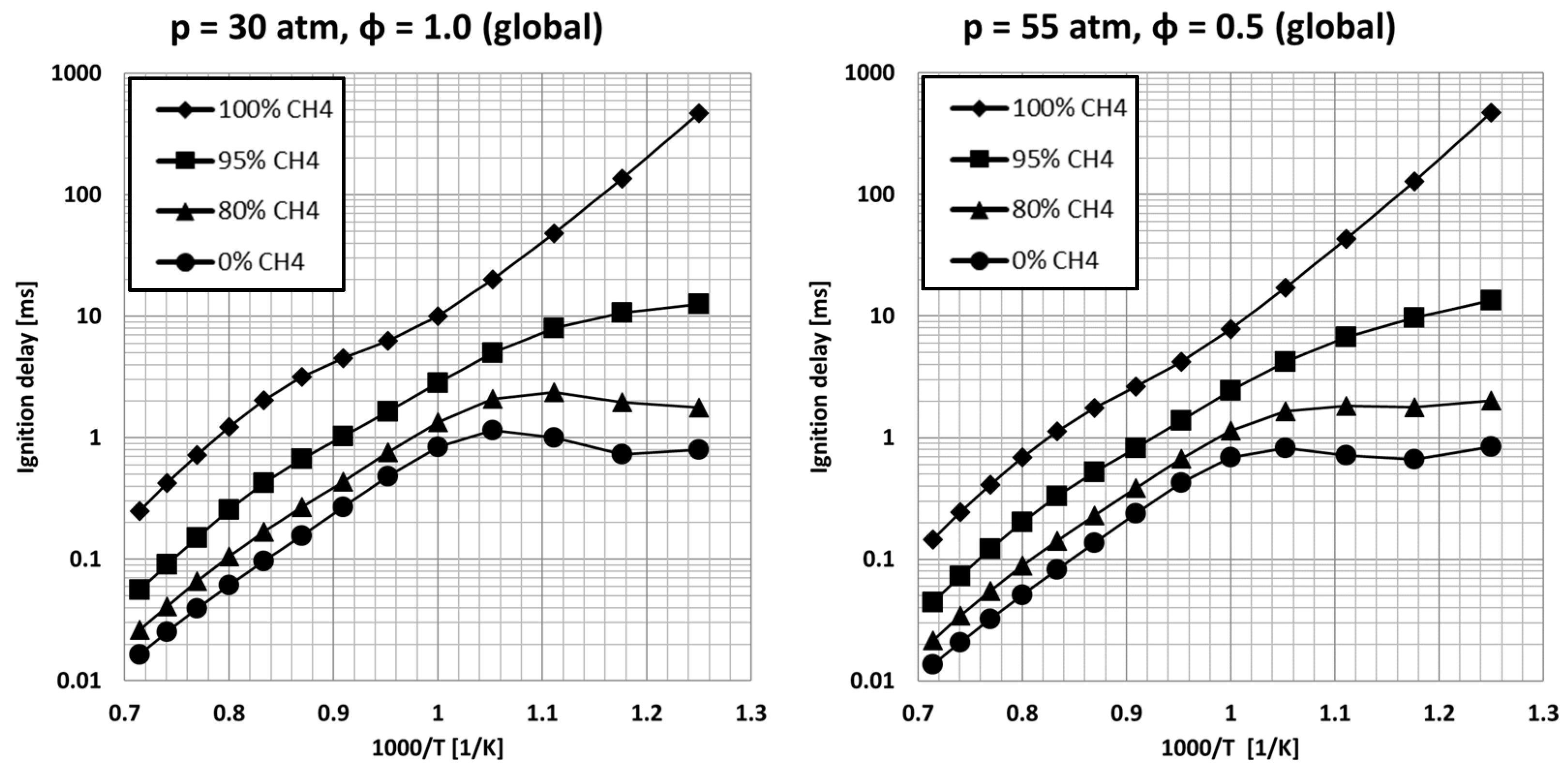
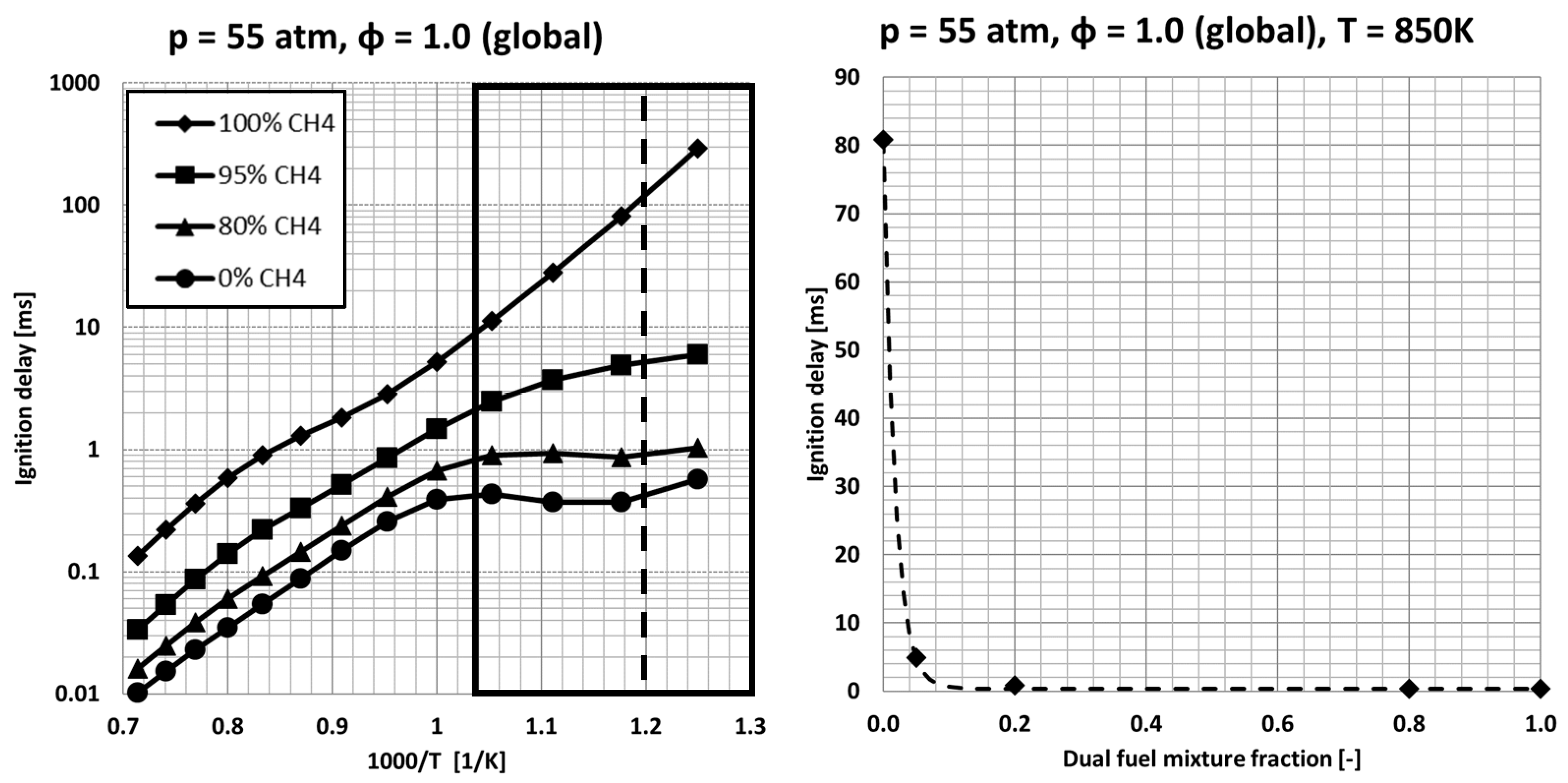
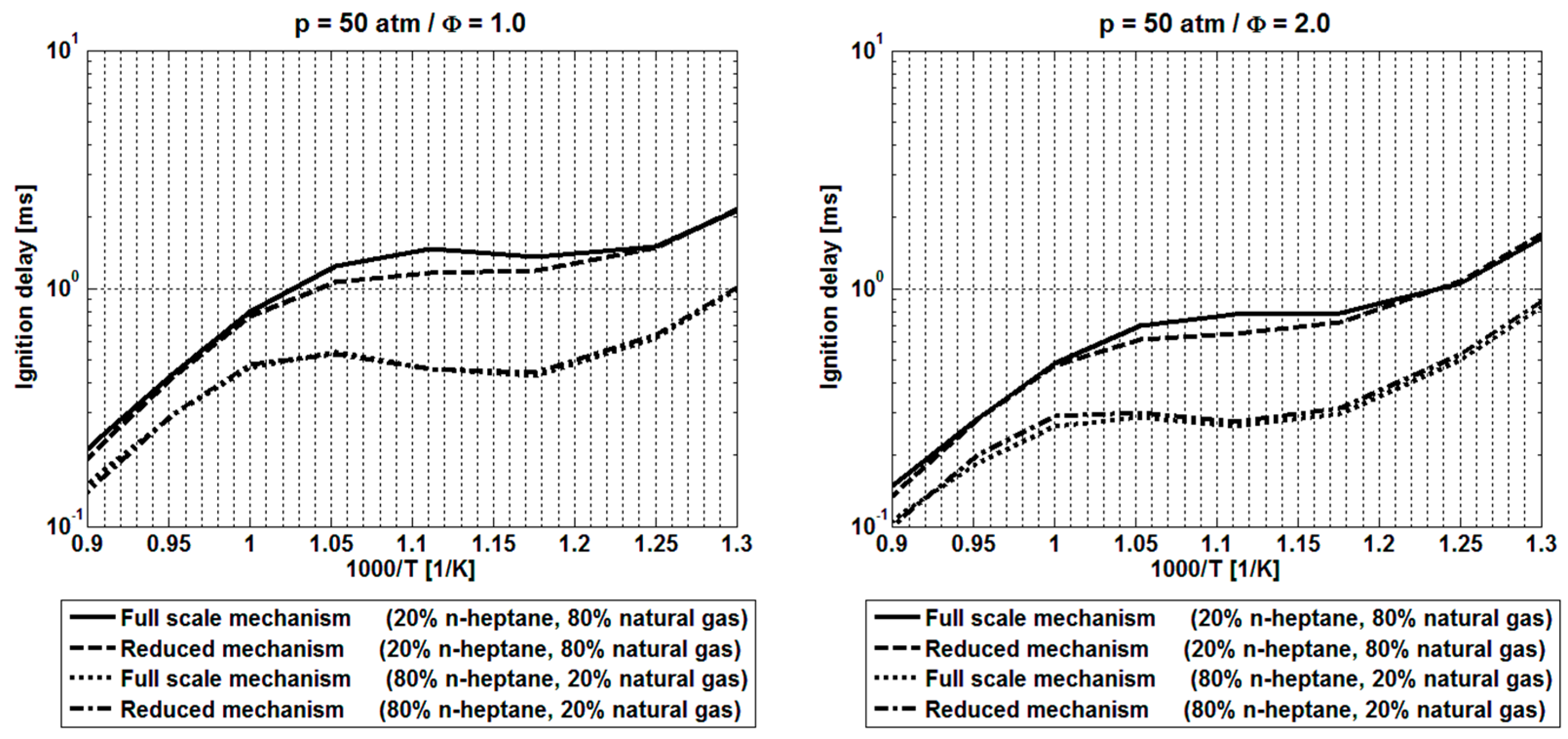
2.2. Ignition Delay Modeling

The first step in modeling ignition delay involves choosing surrogates for the fuels involved. As various compositions of the different species of diesel and natural gas are possible, a chemical surrogate must be selected for both the diesel fuel and the natural gas. One of the best characterized surrogates for diesel fuel is n-heptane—numerous studies show that this surrogate is chemically well understood [55,56,57]. As for natural gas, a combination of methane, ethane, propane and butane is adequate for the applications under investigation. In the following description of the chemical interaction between the two fuels during ignition, n-heptane is chosen as the diesel surrogate and pure methane as the natural gas surrogate.
The next step is to determine which kind of ignition delay modeling can be used. Since the ignition conditions in a diesel ignited gas engine allow cold flame combustion, a numerical modeling approach must be chosen that is able to capture cold flame heat release and the main ignition. An accurate numerical description of ignition delay timing can be achieved by using two-stage tabulation. In this numerical approach, the cold flame ignition delay and the main flame ignition delay are tabulated with respect to pressure, temperature, equivalence ratio and exhaust gas recirculation (EGR) rate. The descriptions provided below show the calculation of just one ignition delay time; this approach can be used for both cold flame and hot flame ignition delay.
After the fuel surrogates and numerical description are determined, the modeling approach considers the interaction of the fuels. As previously mentioned, experimental research [38,39] has revealed that there is a strong interaction between fuels used together in a Rapid Compression Expansion Machine (RCEM). The qualitative behavior of these experiments was also seen in the numerical approaches in [40,41]. 0D simulation carried out with the mechanism used below for dual fuel tabulation shows that there is strong non-linear behavior between the two fuels during ignition. 3 graphs ignition delay with selected pressure and global equivalence ratios versus temperature. The lines in the Figure 3 represent different fuel blends (note that the global equivalence ratio stays the same while the composition of the fuels changes; e.g., 95% CH4 indicates that if the global equivalence ratio is 1, 95 mole percent of the fuel is methane and 5 mole percent is n-heptane).
The strong non-linear behavior of ignition delay versus temperature has to be taken into account in ignition delay modeling of the fuels. This behavior can be captured by one of the following two approaches.
The first approach applies an interpolation function if the ignition delay of each of the fuels has been tabulated with a different reaction mechanism. With a non-linear blending function, these two delays are combined to yield a dual fuel ignition delay.
A second and more accurate approach is to use a specific dual fuel mechanism as described in [45] and examined in more detail in the following subsections to tabulate the ignition delay with respect to temperature T , pressure p , global equivalence ratio Φ g l o b a l and EGR rate x E G R as well as the dual fuel fraction φ D F . The schematic in Figure 4 shows these two approaches.
Both approaches are not limited to the fuel surrogates that have been described, yet adding a new surrogate (e.g., another natural gas component) requires a new tabulation. The following subsections describe each approach in detail, indicating their potential advantages and disadvantages.

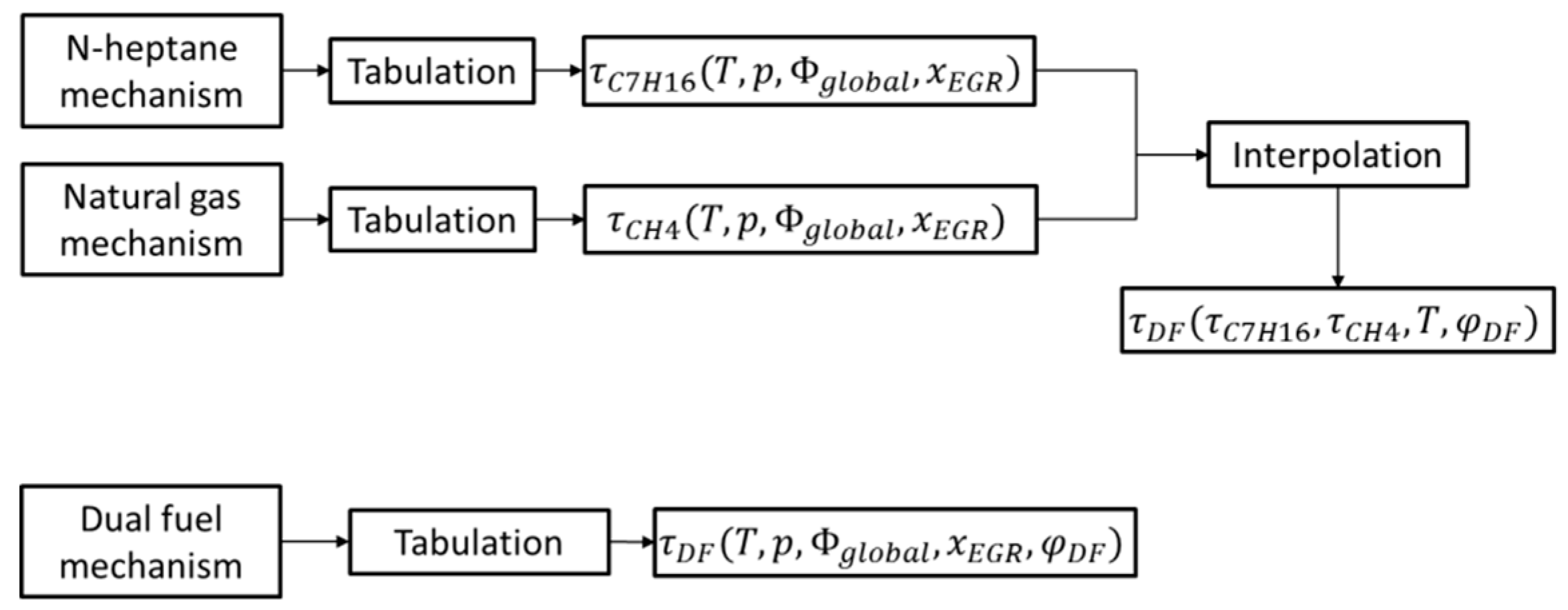
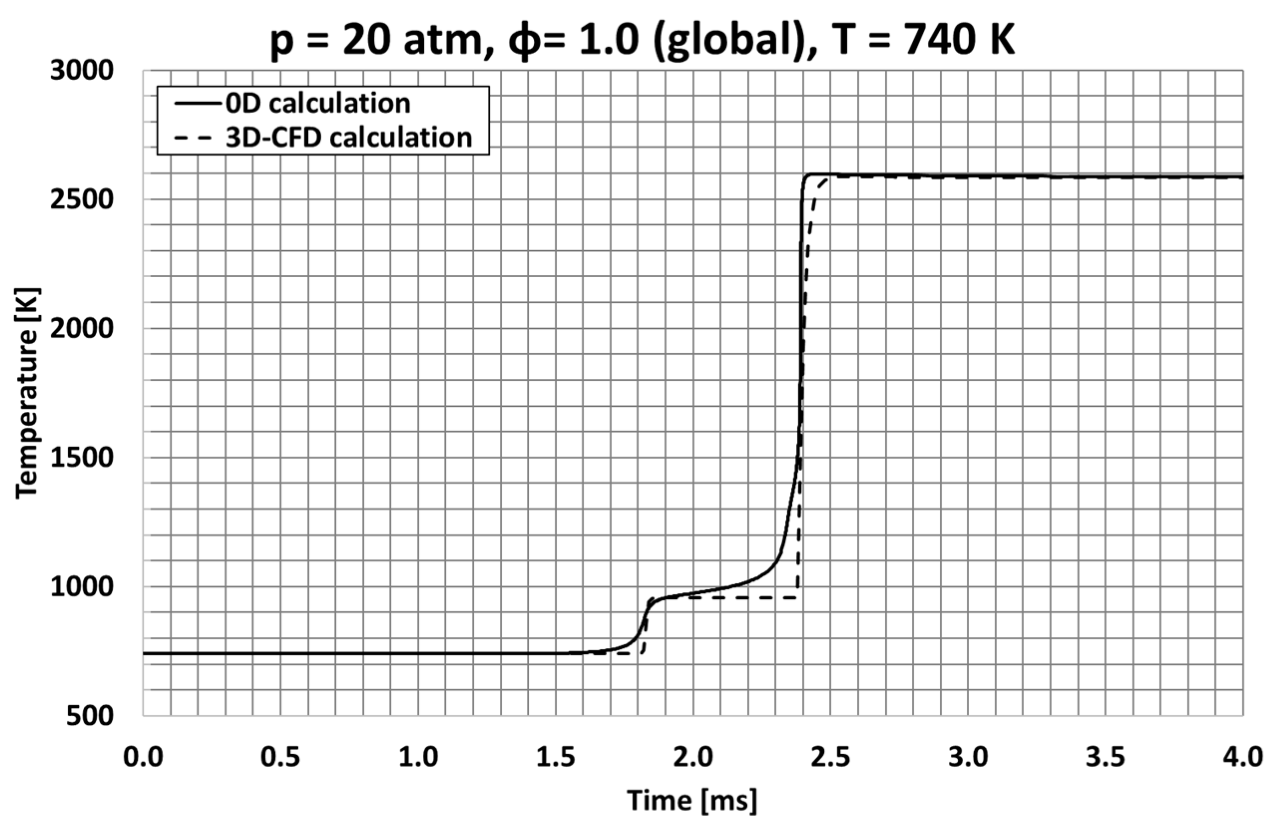
2.3. Two-Stage Ignition with an Interpolation Function

As described in Figure 4, this approach combines two different tables with an interpolation function that is dependent on temperature and the dual fuel mixture fraction φ D F as described in Equation (4):
φ D F =   ν C 7 H 16 ν C 7 H 16 + ν C H 4
where ν C 7 H 16 is the mole fraction of n-heptane and ν C H 4 is the mole fraction of methane. Measurement data from a SCE shows that the injected diesel fuel usually ignites at a temperature below 1000 K. Therefore, it is not necessary that the interpolation function mentioned above covers the whole temperature range. The ignition delay of the individual fuels was tabulated using the LLNL-v3 mechanism for n-heptane [56] and the GRI 3.0 mechanism for natural gas [58]. Equation (5) shows the blending function used to obtain the dual fuel ignition delay with respect to the ignition delay of n-heptane τ C 7 H 16 , the ignition delay of methane τ C H 4 , temperature T and dual fuel mixture fraction φ D F :
τ D F = τ C 7 H 16 × ( 1 e B ( T ) × φ D F ) +   τ C H 4 × e B ( T ) × φ D F
The parameter B(T) is obtained by a mathematical equation based on 0D calculations at a given pressure of 55 atm and a global equivalence ratio of one. The selected case and the temperature range used for the fit is indicated by the black rectangle in Figure 5.
A temperature is then selected (dashed line in left graph) and the 0D calculation data for this point is shown along with the interpolation function (dashed line in the right graph). The interpolation function shows good agreement with the 0D data.
This approach allows the combination of the arbitrary delay times of the two different fuels. One great disadvantage of this interpolation approach, however, is that only the influence of temperature is considered while changes due to pressure, equivalence ratio and EGR rate are not. This non-linear interaction can be depicted more accurately by using a specific dual fuel mechanism for the tabulation and introducing the dual fuel mixture fraction as an additional tabulation dimension.

2.4. Two-Stage Ignition with a Specific Dual Fuel Mechanism

For this approach, it is imperative to have a mechanism that is able to give accurate information on the ignition delay of the fuels involved, especially for the case in which both fuels interact with each other. Such a mechanism was developed by combining one mechanism for n-heptane [59] and one for natural gas [60]. The full scale mechanism was then reduced using numerical approaches as outlined in [37,61]. Further information on the selection of the separate mechanisms as well as the reduction process is provided in [45]. Figure 6 shows the ignition delay of the reduced mechanism compared to the full scale mechanism.
To the best of the authors’ knowledge, no experimental data on dual fuel ignition delays is currently available; only the specific operating conditions of the two mechanisms were compared. The results show that the reduced mechanism is also able to reproduce the ignition delay with satisfactory accuracy. Furthermore, the validation of the measurements of laminar flame speeds is shown. Figure 7 compares the full scale mechanism and the reduced mechanism, whereas Figure 8 provides the results of the reduced mechanism in relation to the experimental data found in [44]. As the laminar flame speed might also be the subject of tabulation in future research, this underlines the fact that the same mechanism can tabulate dual fuel ignition delay as well as laminar flame speed.
In order to improve the accuracy of this approach, a separate database was created with a comprehensive chemical mechanism that includes 695 species and 3037 reactions. A specific dual fuel tabulation procedure (cf. Figure 4) was applied. An additional tabulation parameter was introduced that was defined by applying Equation (4) from the previous section (dual fuel mixture fraction).
By varying the initial parameters, a total of 91,350 0D calculations were performed and post-processed in order to store the low temperature ignition delay time, the main ignition delay time, and respective heat release, which was used to determine the amount of fuel consumed during low temperature ignition (if applicable).
The introduction of a new parameter increased the order of the interpolation database from four to five dimensions, necessitating the adaptation of the previous interpolation routine. A new step was added to obtain the final value of each of the tabulated variables. Initially, the 4D interpolation routine returned a scalar for each of the values required by the combustion model. Increasing the order of the matrix caused the returned values to be vectors, whose size was determined by the number of fuel mixture fraction points. The vectors were processed by a separate interpolation function that returns the final scalar. It should be noted that a linear interpolation was used and proved to be adequately accurate. Since the dependence of the stored data on each of the parameters is far from linear, the distribution of data points was chosen so as to ensure that interpolation would not be one of the governing influences on the returned values. A simple option to improve the accuracy (if necessary) of the interpolation is to run the routine over a series transformed by a logarithmic function and the returned resulting scalar by an exponential function. The concept that makes use of the tabulated values is shown in Figure 9.
In the figure below, the temperature curve calculated with the complex chemistry mechanism (solid curve) and the one obtained with 3D-CFD calculation of a simple cube domain consisting of 27 cells (dashed line) show good agreement.
The two-stage ignition model includes a tracking ignition progress variable and a fuel tracer variable; fuel is consumed rapidly when the tracked values reach the tabulated ignition delays. At low temperature ignition, the amount of fuel consumed relates to the ratio of tabulated heat releases, while at main ignition, it is simply the remainder of the fuel that is consumed.

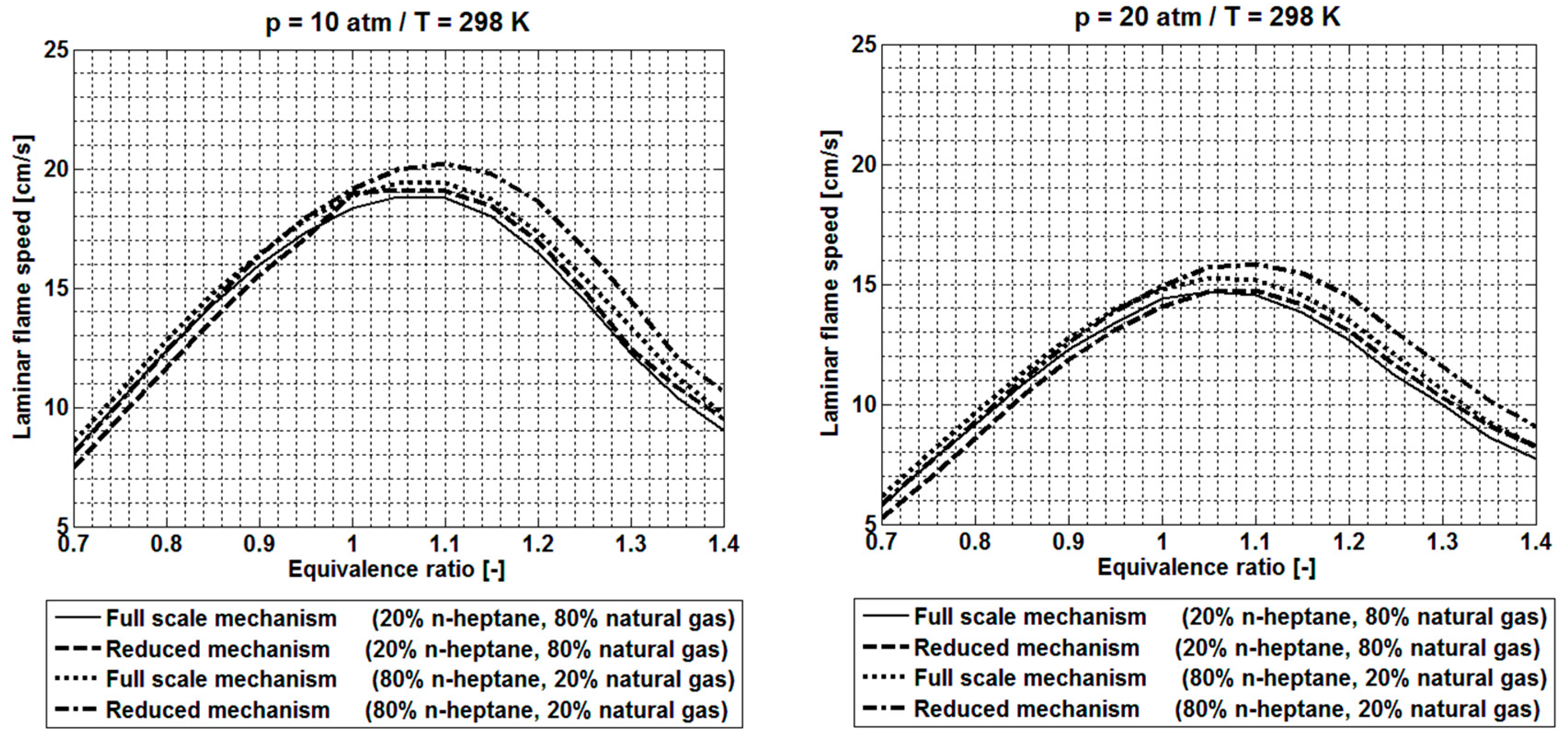
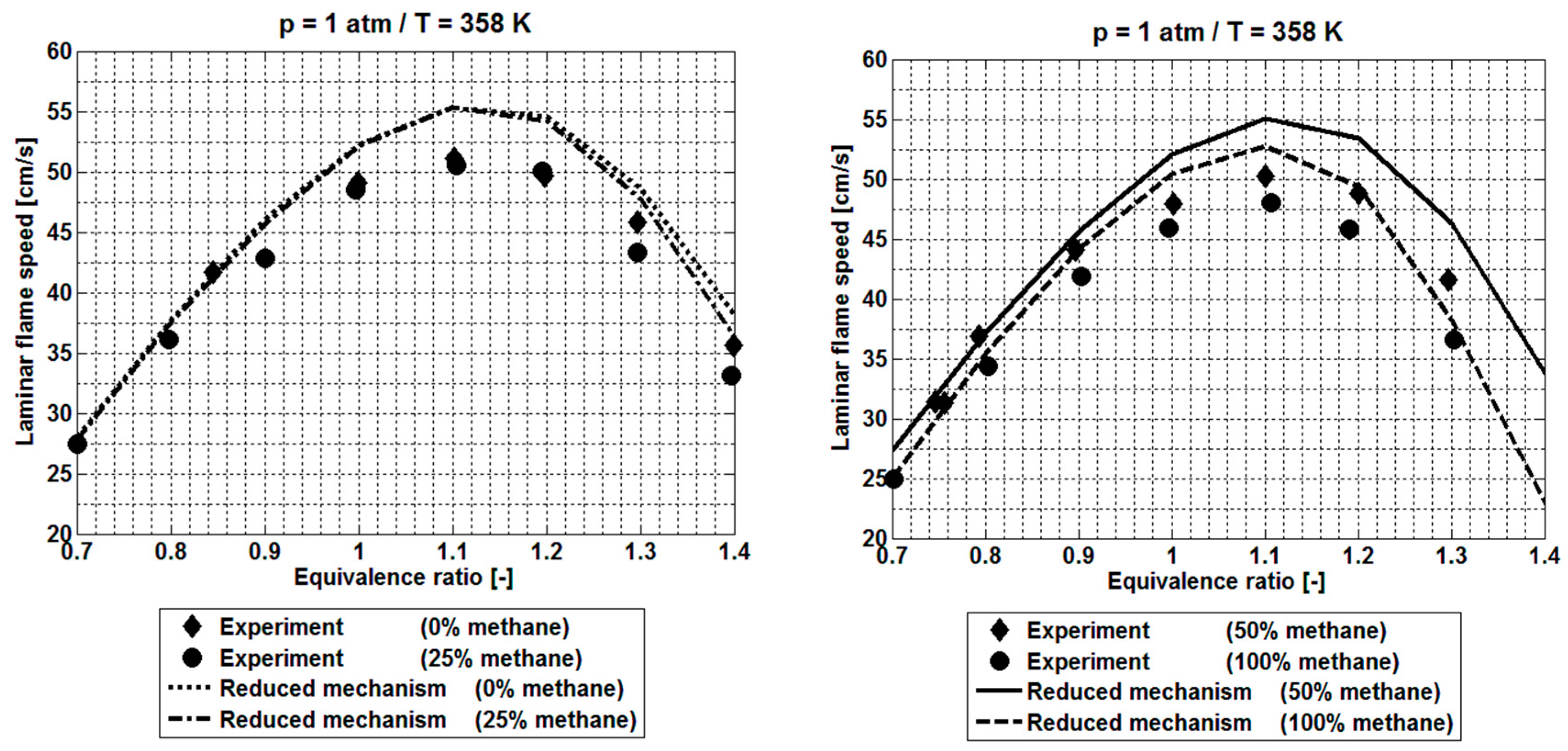
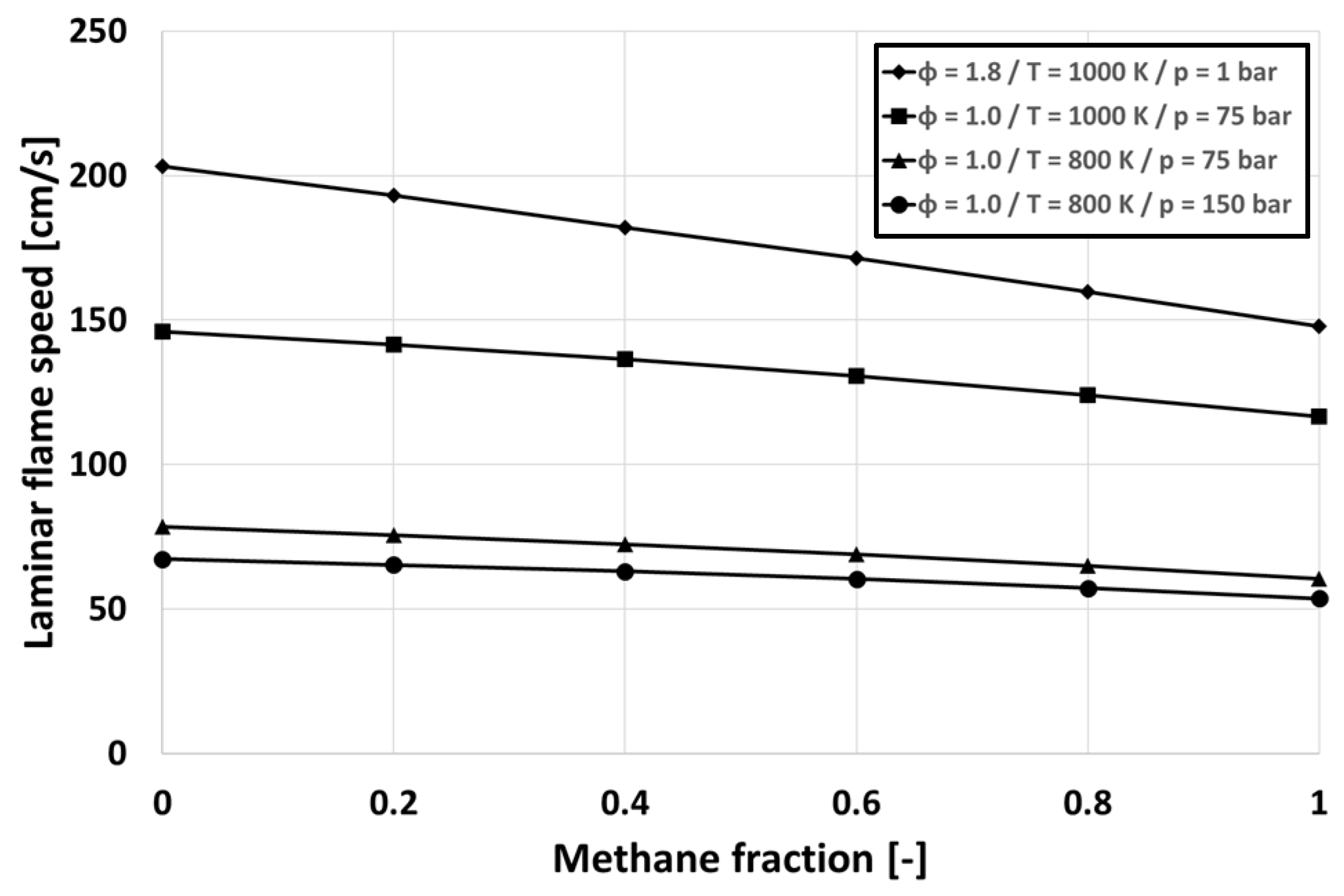
2.5. Premixed Flame Propagation Modeling

As soon as autoignition has occurred, a flame kernel develops and the premixed flame front propagation in the natural gas-air mixture can start. The heat release rate for this regime is calculated by the coherent flame model framework, which assumes decoupled chemistry and turbulence:
ω ˙ ˜ F C F M =   ρ ¯ u × Y ˜ T F ×   s L O ×   Σ
The Reynold’s averaged density in the fresh gases is written as ρ ¯ u ; Y ˜ T F is the tracer fuel mass fraction. The term s L O corresponds to the unstretched laminar flame speed of the fuel. This variable represents the chemical influence of the heat release rate. Special treatment of this variable is required when the diesel ignited gas engine is simulated; it will be described in the next section. Σ is the flame surface density, which represents the influence of turbulence on the combustion. The turbulence only wrinkles and therefore expands the laminar flame surface. This is described by the transport equation for the flame surface density, which is noted as follows:
Σ t +   δ u ˜ i Σ δ x i =   x i   ( ( μ t S c t + μ S c ) x i ( Σ ρ ¯ )   )   + ( P 1 + P 2 + P 3 D ) × Σ
The equation considers convection, diffusion and temporal evolution of the flame surface density as well as several source and sink terms indicated by P 1 ,   P 2 , P 3   and D . As these terms are not investigated separately in this paper, they will not be explained in detail; cf. the original paper by Colin [32] for the ECFM framework and the description of the flame surface density balance equation. The ECFM requires starting values for the progress variable and for the initial flame surface density. The progress variable can be obtained either via the tracer fuels in the two-stage autoignition interpolation or directly from the tables in the case of the TKI tabulation [28]. The initial flame surface density needs additional considerations. Initially proposed by Colin [32] for knock modeling and later used for dual fuel applications by Belaid-Saleh et al. [31], the gradient of the progress variable is represented by:
Σ i n i = | c ˜ |
As Belaid-Saleh describes, this formula is insufficient to properly model the initial flame surface density. The influences of turbulent wrinkling as well as the regime transition from autoignition to flame front propagation have to be considered [31]. As a result, an additional constant is added to the formula as well as the turbulent intensity, which is composed of the turbulent kinetic energy k and the average velocity u ¯ that can further fold the flame kernel:
Σ i n i = C × | c ˜ | × ( 1 +   k u ¯ )
The constant C can take values between 0 and 1 just as Belaid-Saleh explains and can be seen as an adjustment for the regime transition.
As the flame now propagates throughout the mixture, the heat release is calculated according to ω ˙ ˜ F C F M as described in the previous section. The unstretched laminar flame speed s L O must also be considered. If the ignition delay time after the diesel is injected is long as a result of early injection or a very lean background mixture, there is a long time during which the diesel can penetrate the combustion chamber. After autoignition has occurred, the flame front encounters zones of premixed diesel, natural gas and air. To take into account the influence of chemistry during flame front propagation as well, the laminar flame speed has to be modified. Figure 10 shows values for the laminar flame speed with respect to the volumetric methane fraction. The calculations were performed under various pressure, temperature and global equivalence ratio conditions.
Unlike the ignition delay calculations, the results for the laminar flame speed of the fuel mixture exhibit linear behavior with respect the fuel mixture fraction. Recent experimental studies carried out by Li [44] support this assumption. The laminar flame speed for n-heptane was tabulated with the LLNL-v3 mechanism and that of methane was tabulated using the GRI 3.0 mechanism for natural gas. To consider the influence of the fuel mixture on the laminar flame speed, a linear interpolation between the two tabulated values can be used. The modified laminar flame speed for the dual fuel application, referred to as s L d f 0 , is written as follows:
s L d f 0 =   s L C 7 H 16 0 × φ d f +   s L C H 4 0 × ( 1   φ d f )
s L C 7 H 16 0 and s L C H 4 0 are the unstretched laminar flame speeds of n-heptane and methane. Both are determined from the tables described above. The tables consider the dependence of pressure, temperature, EGR ratio and global equivalence ratio. φ d f is once again the dual fuel mixture fraction as described in Equation (4).

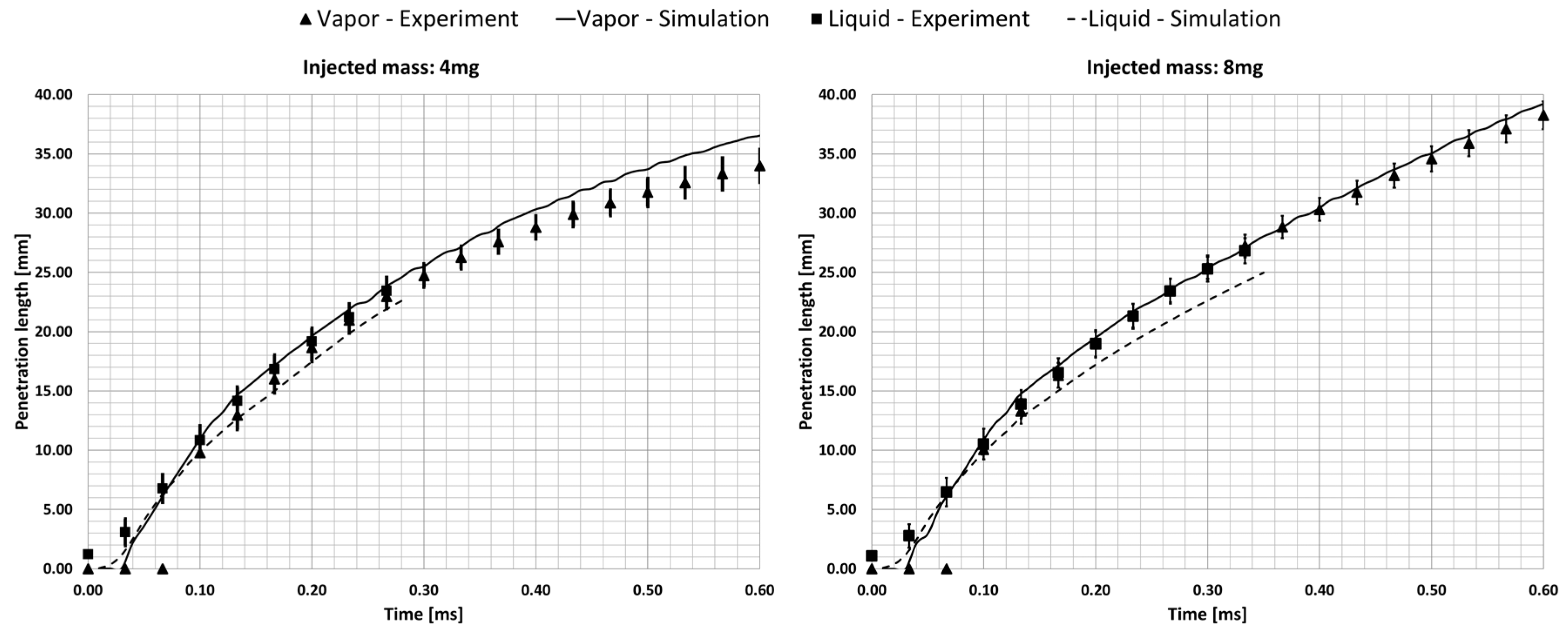
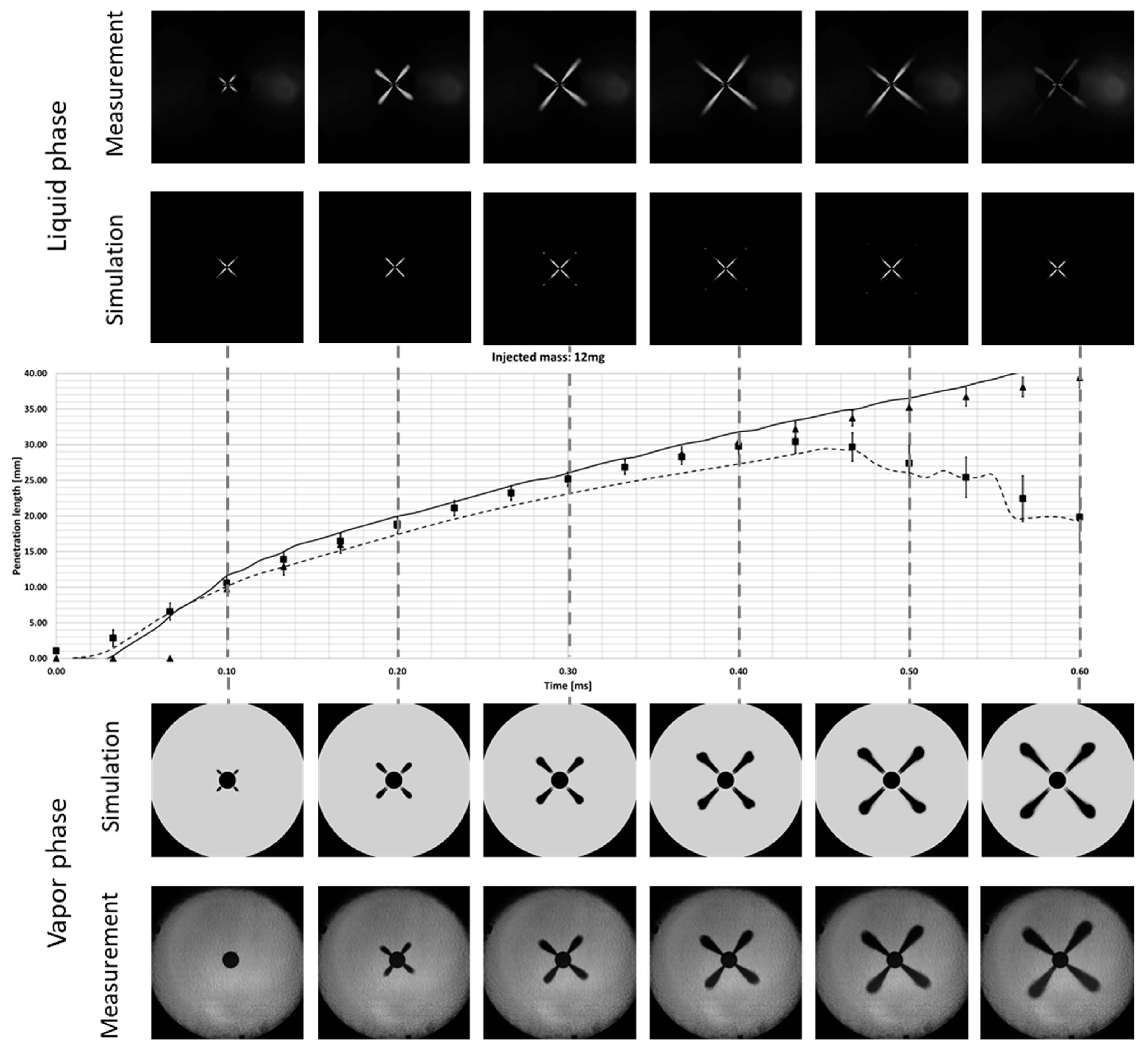
3. Validation of Injection Modeling

This section describes the validation of the injection modeling process discussed above. First, the experimental setup for rate of injection (ROI) measurement is introduced followed by the setup for non-reactive spray visualization. Next, the numerical setup is explained. Selected cases for validation are then presented in which the measured and simulated penetration lengths are compared. Finally, an optical comparison is provided for one selected test case.

3.1. Experimental Setup

A Bosch Tube was used for ROI measurements as described in [62]. The injector sprays the diesel mass into a measurement tube and the ROI is derived from the resulting pressure increase. The vapor and liquid penetration lengths are determined in a chamber filled with gaseous nitrogen. The absence of oxygen prevents combustion. The diesel is injected into a quiescent flow field. Schlieren and Mie scattering measurements are then performed to visualize the vapor and liquid phases of the injected diesel [33]. Further information on the experimental test setup can be found in [63]. A wide range of variations, including chamber temperatures and pressures as well as injection pressures and injected masses, has been tested and validated. Only selected test cases are discussed in this paper. Table 1 provides a short overview of the conditions in the spray chamber that were varied for the validation described in this paper.

3.2. Numerical Setup

The ROI measurements were used directly in the 3D-CFD simulation to accurately set up the spray model. As previously mentioned, the submodels of the spray model include the WAVE breakup model with the model improvements described in the previous section and a Dukowicz evaporation model. For further information on the models, cf. [51]. In addition to the spray model itself, mesh topology, cell size and simulation time step have a significant influence on the predicted spray penetration lengths. The settings for all three factors were similar to the engine mesh described in the following section. Table 2 provides an overview of the numerical setup.

3.3. Validation Cases

Figure 11 shows the measured and simulated vapor and liquid penetration lengths. The vapor penetration length is plotted in triangles; the liquid penetration length is plotted in squares. In both cases, the bars indicate the standard deviation of the measurement fluctuations. The solid line indicates the simulated vapor penetration length, and the dashed line indicates the simulated liquid penetration length.
Reasonable agreement of the penetration lengths is observed in one parameter set that was used in all the selected validation cases. Further validation was carried out using the visualization techniques of the measurement setup. The 3D results from the simulation of a diesel mass of 12 mg were used to recreate the images of the measurement. Figure 12 compares the penetration length once again as shown in the previous figure and also provides images of selected time steps. The top row shows the averaged images of the liquid phase of the measurement. The vertical, grey, dashed lines indicate the according time when the images of measurement and simulation were taken. The second row shows the particles in the simulation. The simulation images have been mirrored from the single spray to mimic the images of the measurement. Therefore, no hole to hole scattering can be seen in the simulation images. The rows of images below the penetration length graph provide the same information about the vapor phase. In the case of simulation, a cut plane is shown that runs through the centerline of the spray; the images show the diesel mass fraction.
The visual comparison shows good agreement between measurement and simulation for the selected test case. One can notice a difference for the liquid phase, which is due to post-processing of the particle diameter in the simulation. The quantitative agreement of the penetration length can still be seen. With this validation process, the spatial resolution of the pilot diesel can be successfully predicted by the simulation. Further validation will now focus on the combustion modeling as described in the previous section, using experimental results from a single cylinder research engine (SCE).

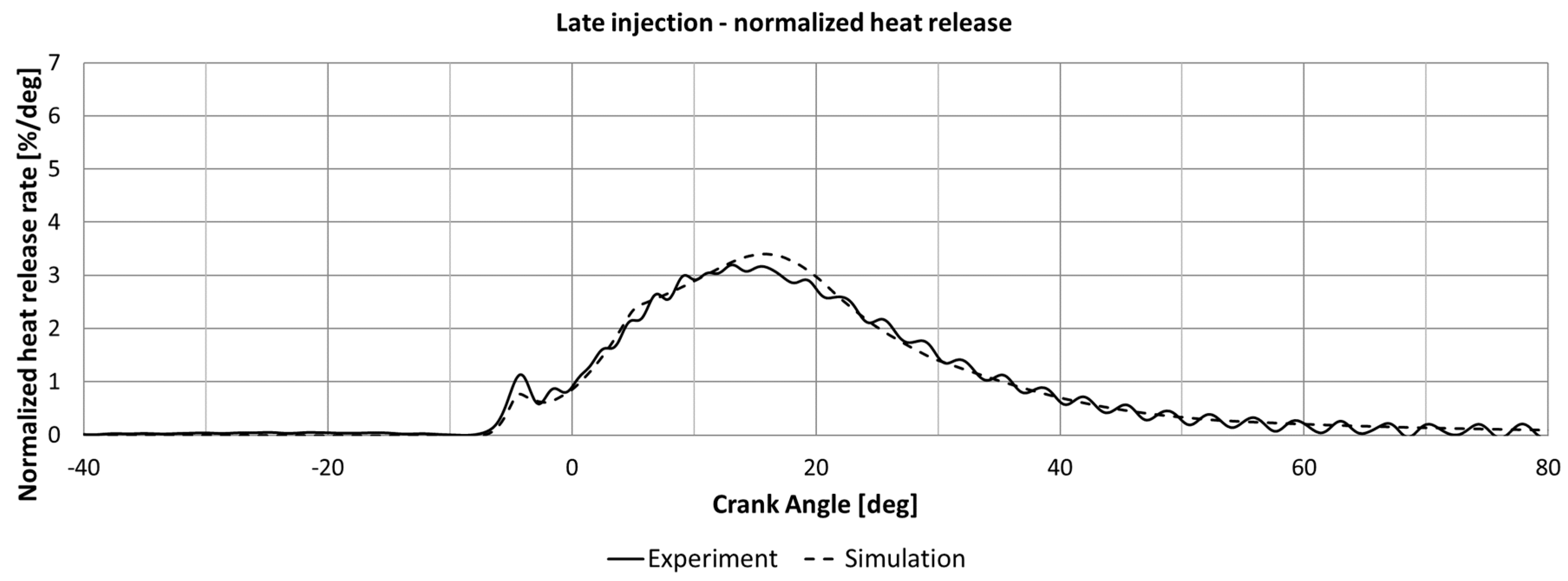
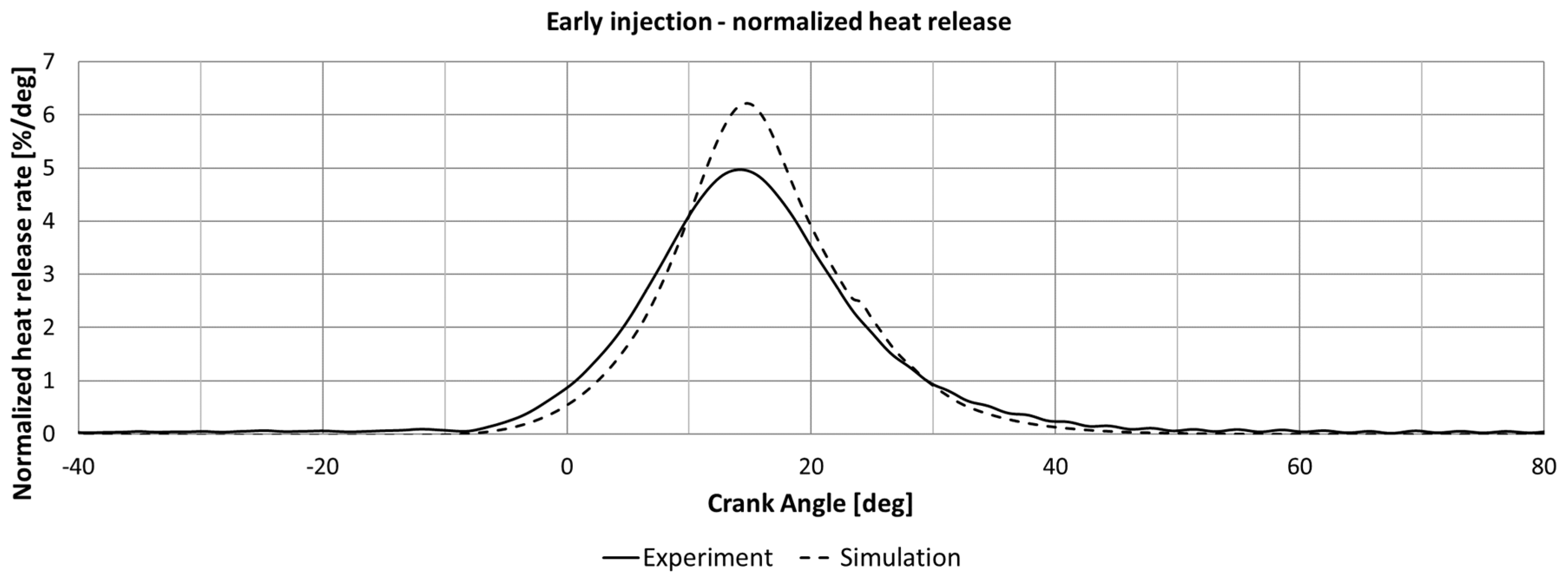
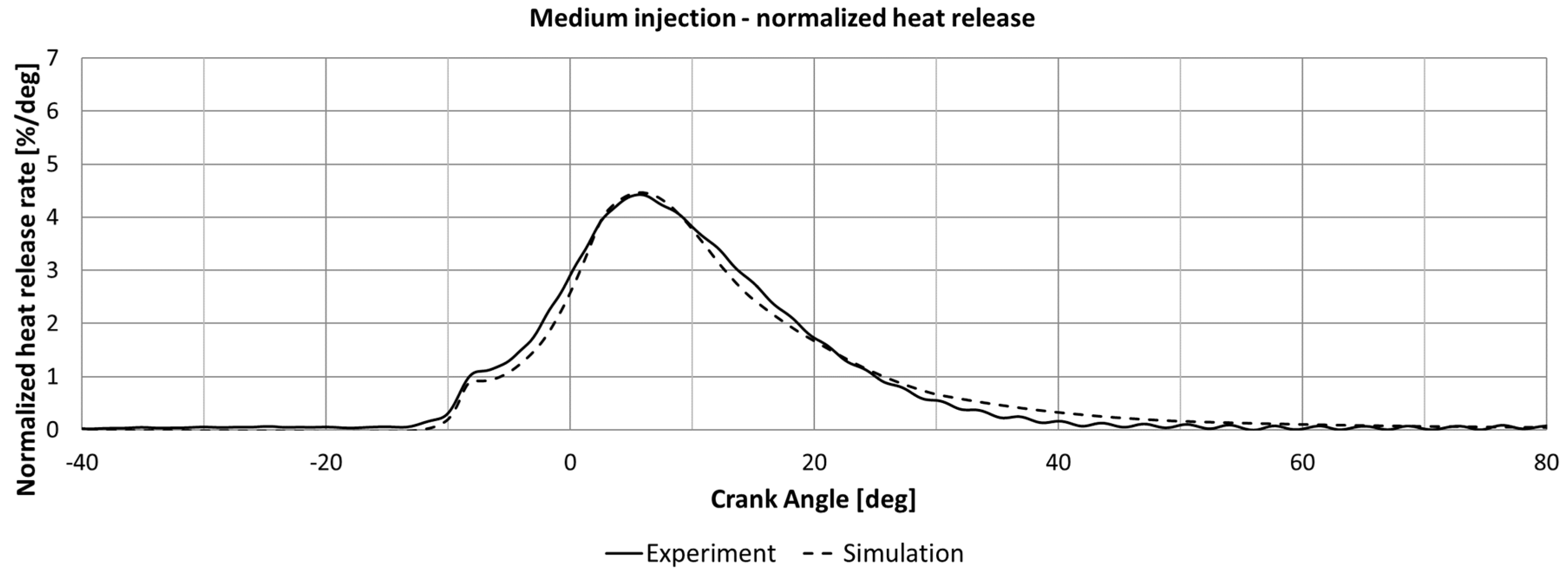
4. Validation of Combustion Modeling

4.1. Experimental Setup

The approach to ignition delay modeling using a dual fuel mechanism as the basis for tabulation was validated using experimental data from a SCE at the LEC in Graz. Table 3 provides relevant engine data along with an image of the SCE. The natural gas-air mixture is prepared in a Venturi mixer several meters upstream of the intake ports, which substantiates the assumption of homogeneous distribution in the combustion chamber. The diesel fuel was injected with a 4-hole injector nozzle with a common rail system. Further information on the measurement setup can be found in [17]. All measurements have been carried out without the use of EGR.

4.2. Numerical Setup

The 3D-CFD simulations only covered the high pressure phase of the working cycle. A 90 degree sector mesh was used for the simulation, cf. Table 4. The number of cells varied from 20,000 at top dead center (TDC) to 150,000 at bottom dead center (BDC), and the average cell size was 2 mm with a refinement in the spray region. Measured rates of injection (ROI) provided the input for the spray model. The spray submodel parameters were calibrated from optical measurements of injection sprays into inert atmospheres; for further information on the calibration, see [64]. The turbulence model was a k-ζ-f model [65].

4.3. Validation Cases

Two different engine operation condition variations were chosen for validation. The first variation is represented by the start of current (SoC). The SoC of the common rail injector was varied by ±10° CA related to a baseline timing. These cases correspond to the first three rows in Table 5. The second variation was in diesel mass, whereby the selected diesel shares of 1.5%, 1.0% and 0.5% correspond to the diesel masses injected shown in the section on the injection modeling variation. Further information on the measurement setup can be found in [65].
At first, the SoC variation is shown in Figure 13. Figure 13 below shows the pressure trace of the average pressure cycle of 100 experimental cycles as well as the maximum and minimum pressure cycles of these cycles. The black dashed line represents the pressure curve from 3D-CFD simulation. The graph on the right shows the normalized heat release rate (HRR) from measurement and simulation. It is clear that when injection timing is early, the ignition delay is well depicted. The predicted heat release rate due to flame front propagation through the natural gas air mixture is higher than the measured heat release rate.
With medium injection timing, which can be seen as the baseline timing, the new ignition delay tables also correctly predict ignition delay and the subsequent flame front propagation is correctly captured. When the heat release rate of medium injection timing, as seen in Figure 14, is compared to the rate of early SoC timing, the premixed peak of diesel combustion becomes more significant when SoC timing is shifted to later crank angles.
The effect of the diesel peak on the heat release rate is increased further by moving the SoC to a late crank angle, cf. Figure 15. The ignition delay prediction is also correct in this case.
The diesel mass variation as described in Table 5 is shown for further validation. With the 1.5% diesel mass injected shown in Figure 16.
As the diesel masses injected become smaller, a slightly less developed “diesel peak” is apparent, cf. Figure 17. The modeling of injection and combustion allows accurate reproduction of the heat release rates and pressure traces from the experiment.
The lower diesel peak becomes even more pronounced when the diesel mass injected is the smallest possible that still permits stable ignition at the specific engine conditions as shown in Figure 18.

5. Discussion of Results

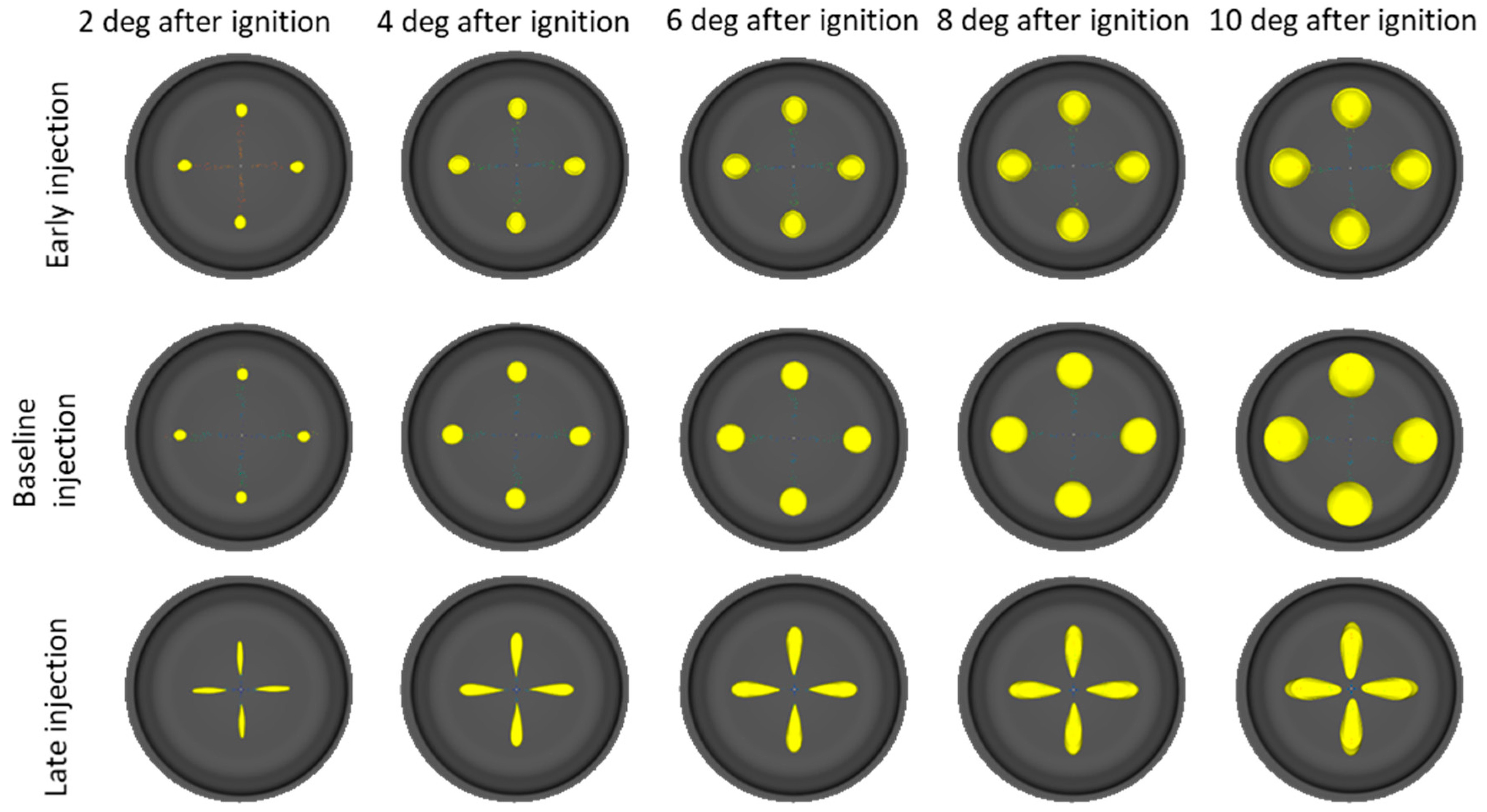
5.1. Injection and Ignition Delay Modeling

The comparison of the simulated and measured vapor and liquid penetration lengths from the selected test cases in Section 3 show reasonable agreement. Furthermore, the qualitative comparison of the post-processed images for measurement and simulation yields satisfactory results. The calibration of the spray model with the diameter specification, therefore, is a valid approach to modeling the pilot injection with the given input data. It should be noted that this is only true when the injector is operated in the ballistic range. With larger diesel masses, where the injector needle reaches and maintains a fully open state for a longer period of time, the calibration approach may no longer be valid. The modeling of the ignition delay Section 2.2 showed reasonable agreement with the SCE results. Currently there are no basic experiments that solely focus on the ignition delay calculation being undertaken, thereby preventing a fundamental investigation of this process.

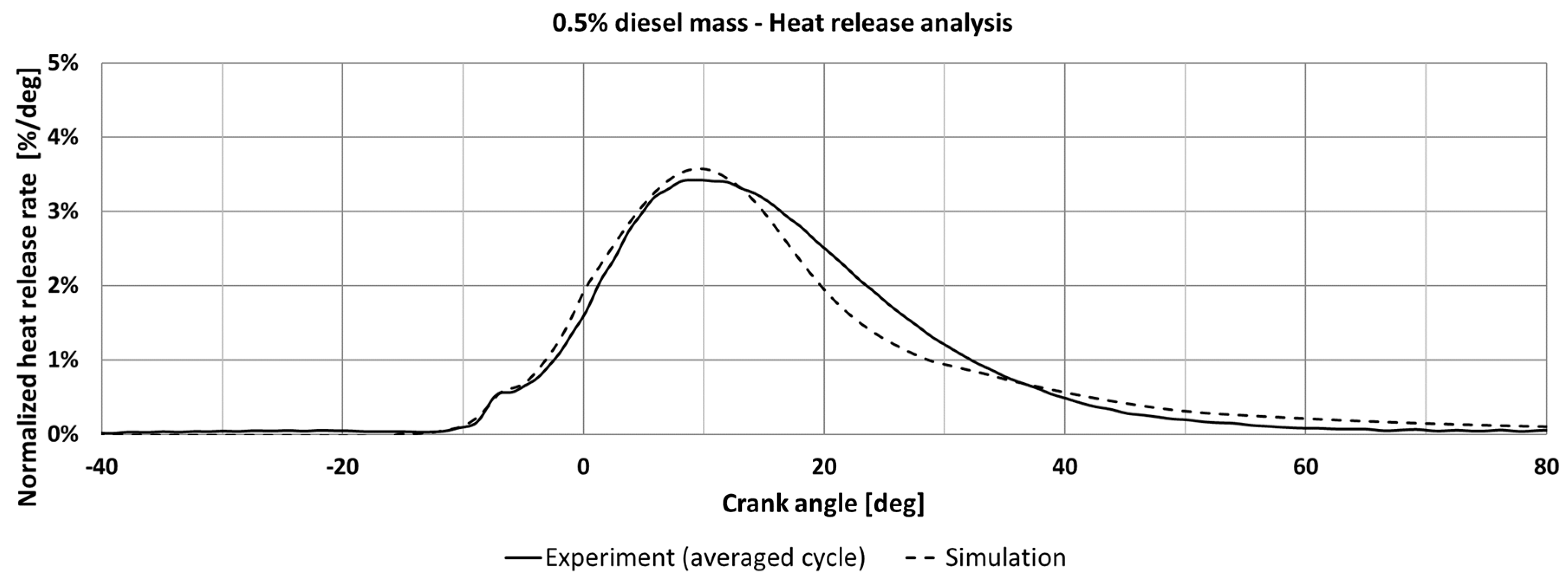
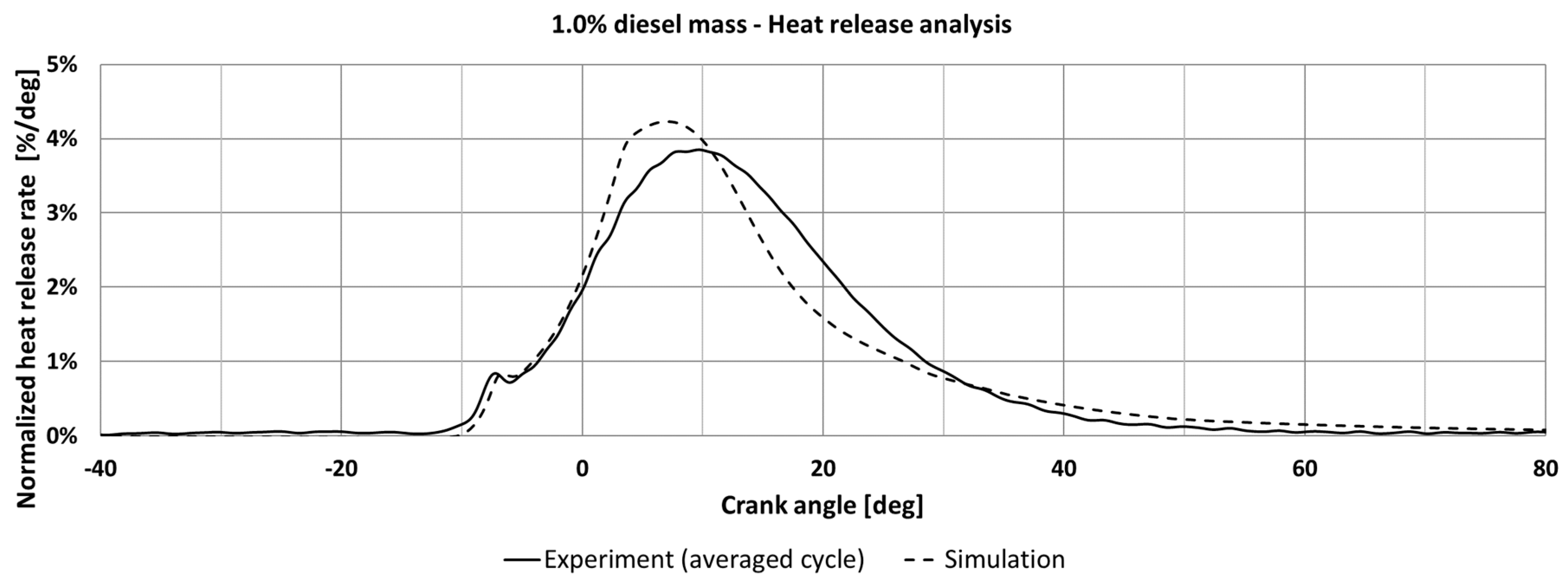
5.2. Combustion Modeling

The overall improvements to the modeling framework of injection, ignition and combustion have been tested on the diesel ignited gas engine concept using results from a single cylinder research engine. The model was able to reproduce the average pressure trace satisfactorily in six selected tests. The further interest of the authors in SoC variation led to a closer analysis of the ignition process in the simulation. Figure 19 shows a top down view into the piston from simulation. Since the sector mesh has been mirrored to mimic the full piston bowl, all spray cones appear to be the same and no hole to hole scattering is observed with this post-processing. The yellow surfaces are isosurfaces of the progress variable, which can be seen as an indicator of where the flame is currently located.
Though this is a qualitative comparison, several basic conclusions can be drawn. At the early injection timing, the diesel fuel has more time to penetrate throughout the combustion chamber and ignites in a rather spherical manner. The later the diesel is injected, the less time there is for mixture formation to occur, which causes the diesel to ignite in more of a conical shape closer to the injector nozzle as with the late injection timing. Although the interpretation seems plausible, it must be compared to the measurements before it can be regarded as a solid argument.

6. Conclusions and Future Work

A comprehensive collection of fundamental experiments regarding diesel pilot injection and single cylinder research engine measurements has led to the development and validation of injection and combustion models to simulate diesel ignited combustion. The results of the inert injection simulations show good agreement regarding liquid and vapor penetration lengths as well as qualitative agreement for visual post-processing. Further work on injection modeling will focus on simulations of a fully opened injector needle as well as reactive simulations. The diesel pilot quantities will be injected into synthetic air to characterize the ignition behavior within the spray box and to generate further data for the validation of the simulation model.
Based on the calibrated spray model for pilot injection, the ignition delay, initial flame surface density deposition and laminar flame speed of dual fuel combustion were able to be simulated with the improved ECFM-3Z model. The results of the simulation show good agreement between simulated and experimental heat release rates. A further analysis of the simulation results has also revealed the plausible behavior of the ignition process. Further work will focus on supporting the assumptions from the 3D-CFD simulation regarding ignition behavior described in Section 5 with endoscopic measurements on the SCE. Modeling efforts will focus on tabulation of the laminar flame speed based on the dual fuel mechanism developed in this paper in order to replace the linear interpolation currently in use. Furthermore, the emissions of the engine, with a special focus on nitric oxides (NOx), soot and unburned hydrocarbons, will be subject of subsequent studies.

Acknowledgments

The authors would like to acknowledge the financial support of the “COMET—Competence Centres for Excellent Technologies Programme” of the Austrian Federal Ministry for Transport, Innovation and Technology (BMVIT), the Austrian Federal Ministry of Science, Research and Economy (BMWFW) and the Provinces of Styria, Tyrol and Vienna for the K1 Centre LEC EvoLET. The COMET Programme is managed by the Austrian Research Promotion Agency (FFG). The authors would like to express their gratitude for the measurement data provided by CMT-Motores Térmicos (Universitat Politècnica de València).

Author Contributions

Lucas Eder, Gerhard Pirker and Andreas Wimmer conceived and designed the experiments/simulations and analyzed the data; Marko Ban and Milan Vujanovic provided the tabulated ignition delays; Peter Priesching provided the software support; Lucas Eder and Gerhard Pirker wrote the paper.

Conflicts of Interest

The authors declare no conflict of interest.

References

  1. Verdolini, E.; Vona, F.; Popp, D. Bridging the Gap: Do Fast Reacting Fossil Technologies Facilitate Renewable Energy Diffusion; National Bureau of Economic Research (NBER): Cambridge, MA, USA, 2016.
  2. International Transport Forum. ITF Transport Outlook 2015; International Transport Forum: Paris, France, 2015. [Google Scholar]
  3. Pirker, G.; Wimmer, A. Sustainable power generation with large gas engines. Energy Convers. Manag. 2017, 149, 1048–1065. [Google Scholar] [CrossRef]
  4. International Maritime Organization. Nitrogen Oxides (NOx)—Regulation 13, 2015. Available online: http://www.imo.org/en/OurWork/Environment/PollutionPrevention/AirPollution/Pages/Nitrogen-oxides-(NOx)-–-Regulation-13.aspx (accessed on 12 September 2016).
  5. Buchholz, B. Saubere Großmotoren für die Zukunft—Herausforderung für die Forschung. In Rostock Large Engine Symposium; FVTR: Rostock, Germany, 2014. [Google Scholar]
  6. Zelenka, J.; Kammel, G. The Quality of Gaseous Fuels and Consequences for Gas Engines. In Proceedings of the 10th Internationale Energiewirtschaftstagung (IEWT 2017), Vienna, Austria, 15–17 February 2017; pp. 1–16. [Google Scholar]
  7. Aaltonen, P.; Järvi, A.; Vaahtera, P.; Widell, K. Paper No. 251: New DF Engine Portfolio (Wärtsilä 4-Stroke). In Proceedings of the 28th CIMAC World Congress, Helsinki, Finland, 6–10 June 2016. [Google Scholar]
  8. Dillen, E.; Yearce, D.; Trask, L.; Klingbeil, A. Paper No. 214: GE Transportation Dual Fuel Locomotive Development. In Proceedings of the 28th CIMAC World Congress, Helsinki, Finland, 6–10 June 2016. [Google Scholar]
  9. Issei, O.; Nishida, K.; Hirose, K. Paper No. 049: New marine gas engine development in YANMAR. In Proceedings of the 28th CIMAC World Congress, Helsinki, Finland, 6–10 June 2016. [Google Scholar]
  10. Yoon, W. Paper No. 201: Development of HiMSEN Dual Fuel Engine Line-up. In Proceedings of the 28th CIMAC World Congress, Helsinki, Finland, 6–10 June 2016. [Google Scholar]
  11. Energy Information Administration (EIA). Available online: https://www.eia.gov/dnav/ng/NG_PRI_FUT_S1_M.htm (accessed on 2 February 2018).
  12. Mooser, D. Brenngase und Gasmotoren. In Handbuch Dieselmotoren, 3rd ed.; Aufl, K., Mollenhauer, K., Tschöke, H., Eds.; Springer: Berlin/Heidelberg, Germany, 2007. [Google Scholar]
  13. Redtenbacher, C.; Kiesling, C.; Wimmer, A.; Sprenger, F.; Fasching, P.; Eichelseder, H. Dual Fuel Brennverfahren—Ein zukunftsweisendes Konzept vom PKW-bis zum Großmotorenbereich? In Proceedings of the 37th International Vienna Motor Symposium, Vienna, Austria, 28–29 April 2016; pp. 403–428. [Google Scholar]
  14. Krenn, M.; Redtenbacher, C.; Pirker, G.; Wimmer, A. A new approach for combustion modeling of large dual-fuel engines. In Proceedings of the Heavy-Duty, On- und Off-Highway Engines 2015—10th International MTZ Conference, Speyer, Germany, 24–25 November 2015; pp. 1–19. [Google Scholar]
  15. Königsson, F. On Combustion in the CNG—Diesel Dual Fuel Engine. Ph.D. Thesis, KTH Royal Institute of Technology, Stockholm, Sweden, 2014. [Google Scholar]
  16. Manns, H.J.; Brauer, M.; Dyja, H.; Beier, H.; Lasch, A. Diesel CNG—The Potential of a Dual Fuel Combustion Concept for Lower CO2 and Emissions; SAE International: Warrendale, PA, USA, 2015. [Google Scholar]
  17. Redtenbacher, C.; Kiesling, C.; Malin, M.; Wimmer, A.; Pastor, J.V.; Pinotti, M. Potential and Limitations of Dual Fuel Operation of High Speed Large Engines. In Proceedings of the ASME 2016 Internal Combustion Fall Technical Conference, San Diego, CA, USA, 4–7 November 2018. [Google Scholar]
  18. Hanenkamp, A.; Böckhoff, N. The 51/60 DF and V32/40 PGI—Modern Gas engines from MAN Diesel SE. Their way from development to serial application. In Proceedings of the 6th Dessauer Gasmotoren-Konferenz, Dessau-Roßlau, Germany, 26–27 March 2009; pp. 129–142. [Google Scholar]
  19. Troberg, M.; Portin, K.; Jarvi, A. Paper No. 406: Update on Wärtsilä 4-stroke Gas Product Development. In Proceedings of the 27th CIMAC World Congress, Shanghai, China, 13–16 May 2013. [Google Scholar]
  20. Böckhoff, N.; Mondrzyk, D.; Terbeck, S. Continuous Development of the 51/60G to the 51/60G TS of the MAN Diesel and Turbo SE. In Proceedings of the 10th Dessauer Gasmotoren-Konferenz, Dessau-Roßlau, Germany, 6–7 April 2017; pp. 61–71. [Google Scholar]
  21. Donateo, T.; Carlucci, A.P.; Strafella, L.; Laforgia, D. Experimental Validation of a CFD Model and an Optimization Procedure for Dual Fuel Engines; SAE International: Warrendale, PA, USA, 2014. [Google Scholar]
  22. Hockett, A.; Hampson, G.; Marchese, A.J. Development and Validation of a Reduced Chemical Kinetic Mechanism for Computational Fluid Dynamics Simulations of Natural Gas/Diesel Dual-Fuel Engines. Energy Fuels 2016, 30, 2414–2427. [Google Scholar] [CrossRef]
  23. Maghbouli, A.; Saray, R.K.; Shafee, S.; Ghafouri, J. Numerical study of combustion and emission characteristics of dual-fuel engines using 3D-CFD models coupled with chemical kinetics. Fuel 2013, 106, 98–105. [Google Scholar] [CrossRef]
  24. Mousavi, S.M.; Saray, R.K.; Poorghasemi, K.; Maghbouli, A. A numerical investigation on combustion and emission characteristics of a dual fuel engine at part load condition. Fuel 2016, 166, 309–319. [Google Scholar] [CrossRef]
  25. Li, Y.; Guo, H.; Li, H. Evaluation of Kinetics Process in CFD Model and Its Application in Ignition Process Analysis of a Natural Gas-Diesel Dual Fuel Engine; SAE International: Warrendale, PA, USA, 2017. [Google Scholar]
  26. Maurya, R.K.; Mishra, P. Parametric investigation on combustion and emissions characteristics of a dual fuel (natural gas port injection and diesel pilot injection) engine using 0-D SRM and 3D CFD approach. Fuel 2017, 210, 900–913. [Google Scholar] [CrossRef]
  27. Colin, O.; Benkenida, A. The 3-Zones Extended Coherent Flame Model (ECFM3Z) for Computing Premixed/Diffusion Combustion. Oil Gas Sci. Technol. 2004, 59, 593–609. [Google Scholar] [CrossRef]
  28. Colin, O.; da Cruz, A.P.; Jay, S. Detailed chemistry-based auto-ignition model including low temperature phenomena applied to 3-D engine calculations. Proc. Combust. Inst. 2005, 30, 2649–2656. [Google Scholar] [CrossRef]
  29. Subramanian, G.; da Cruz, A.P.; Colin, O.; Vervisch, L. Modeling Engine Turbulent Auto-Ignition Using Tabulated Detailed Chemistry; SAE International: Warrendale, PA, USA, 2007; pp. 776–790. [Google Scholar]
  30. Subramanian, G.; Vervisch, L.; Ravet, F. New Developments in Turbulent Combustion Modeling for Engine Design: ECFM-CLEH Combustion Model; SAE International: Warrendale, PA, USA, 2007. [Google Scholar]
  31. Belaid-Saleh, H.; Jay, S.; Kashdan, J.; Ternel, C.; Mounaim-Rousselle, C. Numerical and Experimental Investigation of Combustion Regimes in a Dual Fuel Engine; SAE International: Warrendale, PA, USA, 2013. [Google Scholar]
  32. Colin, O.; Benkenida, A.; Angelberger, C. 3D Modeling of Mixing, Ignition and Combustion Phenomena in Highly Stratified Gasoline Engines. Oil Gas Sci. Technol. 2003, 58, 47–62. [Google Scholar] [CrossRef]
  33. Pastor, J.V.; Payri, R.; Garcia-Oliver, J. Analysis of Transient Liquid and Vapor Phase Penetration for Diesel Sprays under Variable Injection Conditions. At. Sprays 2011, 21, 503–520. [Google Scholar] [CrossRef]
  34. Malalasekera, W.; Versteeg, H.K. An Introduction to Computational Fluid Dynamics—The Finite Volume Method; Pearson Education Limited: London, UK, 1995. [Google Scholar]
  35. Merker, G.P.; Schwarz, C. Grundlagen Verbrennungsmotoren; Vieweg Teubner: Wiesbaden, Germany, 2009. [Google Scholar]
  36. Mastorakos, E. Ignition of turbulent non-premixed flames. Prog. Energy Combust. Sci. 2009, 35, 57–97. [Google Scholar] [CrossRef]
  37. Kuo, K.K.; Acharya, R. Fundamentals of Turbulent Multi-Phase Combustion; John Wiley & Sons: New York, NY, USA, 2012. [Google Scholar]
  38. Schlatter, S.; Schneider, B.; Wright, Y.; Boulouchos, K. Experimental Study of Ignition and Combustion Characteristics of a Diesel Pilot Spray in a Lean Premixed Methane/Air Charge Using a Rapid Compression Expansion Machine; SAE Technical Paper; SAE International: Warrendale, PA, USA, 2012. [Google Scholar]
  39. Schlatter, S.; Schneider, B.; Wright, Y.M.; Boulouchos, K. N-heptane micro pilot assisted methane combustion in a Rapid Compression Expansion Machine. Fuel 2016, 179, 339–352. [Google Scholar] [CrossRef]
  40. Aggarwal, S.K.; Awomolo, O.; Akber, K. Ignition characteristics of heptane–hydrogen and heptane–methane fuel blends at elevated pressures. Int. J. Hydrogen Energy 2011, 36, 15392–15402. [Google Scholar] [CrossRef]
  41. Ban, M.; Vujanovic, M. Investigation of Dual-fuel Combustion Properties for CFD Simulation Purposes. In Proceedings of the 11th Conference on Sustainable Development of Energy, Water and Environment Systems, Lisbon, Portugal, 4–9 September 2016. [Google Scholar]
  42. Demosthenous, E.; Borghesi, G.; Mastorakos, E.; Cant, R.S. Direct Numerical Simulations of premixed methane flame initiation by pilot n-heptane spray autoignition. Combust. Flame 2016, 163, 122–137. [Google Scholar] [CrossRef]
  43. Wang, Z.; Abraham, J. Fundamental physics of flame development in an autoigniting dual fuel mixture. Proc. Combust. Inst. 2015, 35, 1041–1048. [Google Scholar] [CrossRef]
  44. Li, G.; Liang, J.; Zhang, Z.; Tian, L.; Cai, Y.; Tian, L. Experimental investigation on laminar burning velocities and Markstein lengths of premixed methane-n-heptane-air mixtures. Energy Fuels 2015, 29, 4549–4556. [Google Scholar] [CrossRef]
  45. Eder, L.; Kiesling, C.; Pirker, G.; Wimmer, A. Development and Validation of a Reduced Reaction Mechanism for CFD Simulation of Diesel Ignited Gas Engines. SAE Int. J. Fuels Lubr. 2009, 1, 675–702. [Google Scholar]
  46. Heywood, J.B. Internal Combustion Engine Fundementals; McGraw-Hill Education: New York, NY, USA, 1988. [Google Scholar]
  47. Donateo, T.; Strafella, L.; Laforgia, D. Effect of the Shape of the Combustion Chamber on Dual Fuel Combustion; SAE International: Warrendale, PA, USA, 2013. [Google Scholar]
  48. Kuppa, K.; Butzbach, G.; Ratzke, A.; Dinkelacker, F. A Numerical Approach for the Prediction of Unburned Hydrocarbon Emissions in Gas Engines. In Proceedings of the 8th International Seminar on Flame Structure: Flame Structure, Berlin, Germany, 21–24 September 2014. [Google Scholar]
  49. Chevillard, S.; Colin, O.; Bohbot, J.; Wang, M.; Pomraning, E.; Senecal, P.K. Advanced Methodology to Investigate Knock for Downsized Gasoline Direct Injection Engine Using 3D RANS Simulations; SAE International: Warrendale, PA, USA, 2017. [Google Scholar]
  50. Reitz, R.D. Modeling Atomization Processes in High-Pressure Vaporizing Sprays. At. Sprays Technol. 1987, 3, 309–337. [Google Scholar]
  51. AVL. AVL FIRE Spray Module—Version Manual 2014.1; AVL: Graz, Austria, 2014. [Google Scholar]
  52. Dukowicz, J.K. Quasi-Steady Droplet Phase Change in the Presence of Convection; Los Alamos Scientific Laboratory: Los Alamos, NM, USA, 1979.
  53. Roth, H.; Giannadakis, E.; Gavaises, M.; Arcoumanis, C.; Omae, K.; Sakata, I.; Nakamura, M.; Yanagihara, H. Effect of Multi-Injection Strategy on Cavitation Development in Diesel Injector Nozzle Holes. SAE Trans. 2005, 114, 1029–1045. [Google Scholar]
  54. Arcoumanis, C.; Flora, H.; Gavaises, M.; Badami, M. Cavitation in Real-Size Multi-Hole Diesel Injector Nozzle; SAE International: Warrendale, PA, USA, 2000. [Google Scholar]
  55. Curran, H.J. Rate constant estimation for C1 to C4 alkyl and alkoxyl radical decomposition. Int. J. Chem. Kinet. 2006, 38, 250–275. [Google Scholar] [CrossRef]
  56. Conaire, M.Ó.; Curran, H.J.; Simmie, J.M.; Pitz, W.J.; Westbrook, C.K. A comprehensive modeling study of hydrogen oxidation. Int. J. Chem. Kinet. 2004, 36, 603–622. [Google Scholar] [CrossRef]
  57. Mehl, M.; Pitz, W.J.; Westbrook, C.K.; Curran, H.J. Kinetic modeling of gasoline surrogate components and mixtures under engine conditions. Proc. Combust. Inst. 2011, 33, 193–200. [Google Scholar] [CrossRef]
  58. Smith, G.; Bowman, T.; Frenklach, M. “GRI 3.0 Mechanism”, Gas Research Institutue—GRI, 2000. Available online: http://combustion.berkeley.edu/gri-mech/index.html (accessed on 18 November 2016).
  59. Mehl, M.; Chen, J.Y.; Pitz, W.J.; Sarathy, S.M.; Westbrook, C.K. An Approach for Formulating Surrogates for Gasoline with Application toward a Reduced Surrogate Mechanism for CFD Engine Modeling. Energy Fuels 2011, 25, 5215–5223. [Google Scholar] [CrossRef]
  60. Petersen, E.L.; Kalitan, D.M.; Simmons, S.; Bourque, G.; Curran, H.J.; Simmie, J.M. Methane/propane oxidation at high pressures: Experimental and detailed chemical kinetic modeling. Proc. Combust. Inst. 2007, 31, 447–454. [Google Scholar] [CrossRef]
  61. Niemeyer, K.E.; Sung, C.J.; Raju, M.P. Skeletal mechanism generation for surrogate fuels using directed relation graph with error propagation and sensitivity analysis. Combust. Flame 2010, 157, 1760–1770. [Google Scholar] [CrossRef]
  62. Bosch, W. Der Einspritzgesetz-Indikator, ein neues Meßgerät zur direkten Bestimmung des Einspritzgesetzes von Einzeleinspritzungen. Mot. Z. 1964, 25, 268–282. (In German) [Google Scholar]
  63. Kiesling, C.; Redtenbacher, C.; Kirsten, M.; Andreas, W.; Imhof, D.; Berger, J.M. IngmarGarcía-oliver, Detailed Assessment of an Advanced Wide Range Diesel Injector for Dual Fuel Operation of Large Engines. In Proceedings of the CIMAC Congress 2016, Helsinki, Finland, 6–10 June 2016. [Google Scholar]
  64. Eder, L.; Kiesling, C.; Pirker, G.; Priesching, P.; Wimmer, A. Multidimensional Modeling of Injection and Combustion Phenomena in a Diesel Ignited Gas Engine; SAE International: Warrendale, PA, USA, 2017. [Google Scholar]
  65. Hanjalić, K.; Popovac, M.; Hadžiabdić, M. A robust near-wall elliptic-relaxation eddy-viscosity turbulence model for CFD. Int. J. Heat Fluid Flow 2004, 25, 1047–1051. [Google Scholar] [CrossRef]
Figure 1. Numerical challenges for the 3D-CFD simulation of a dual fuel engine. The combustion regimes encountered are shown in the triangle. The red rectangle shows the focus of this paper.
Energies 11 00643 g001
Figure 2. Specification of an inconstant nozzle diameter to modify the injection velocity of the droplets in the simulation model.
Energies 11 00643 g002
Figure 3. Ignition delay times with different fuel blends of n-heptane and methane at fixed global equivalence ratios and pressures.
Energies 11 00643 g003
Figure 4. Schematic of the two proposed approaches for dual fuel ignition delay interpolation.
Energies 11 00643 g004
Figure 5. Selected temperature range (within the black rectangle) for the interpolation function at a given pressure and global equivalence ratio (left); selected interpolation temperature indicated by the dashed line. 0D results and interpolation function for the selected temperature (right).
Energies 11 00643 g005
Figure 6. Comparison of ignition delay calculations for dual fuel mixtures. The full scale dual fuel mechanism is compared to the reduced mechanism.
Energies 11 00643 g006
Figure 7. Comparison of laminar flame speed calculations for dual fuel mixtures. The full scale dual fuel mechanism is compared to the reduced mechanism.
Energies 11 00643 g007
Figure 8. Comparison of laminar flame speed calculations for dual fuel mixtures. The reduced dual fuel mechanism is compared to the experimental data found in [44].
Energies 11 00643 g008
Figure 9. Comparison of 0D calculation with 3D-CFD calculation with tabulated values.
Energies 11 00643 g009
Figure 10. Laminar flame speed calculations for selected operating conditions. Calculations were performed with the full LLNL-v3 n-heptane mechanism. 0 on the x-axis indicates pure n-heptane, 1 indicates pure methane.
Energies 11 00643 g010
Figure 11. Comparison of the numerical and experimental results of selected test cases; 4 mg and 8 mg diesel masses injected.
Energies 11 00643 g011
Figure 12. Visual comparison of simulation and measurement of a 12 mg diesel mass.
Energies 11 00643 g012
Figure 13. Measured and simulated heat release rates, early injection timing.
Energies 11 00643 g013
Figure 14. Measured and simulated rates, medium injection timing.
Energies 11 00643 g014
Figure 15. Measured and simulated heat release rates, late injection timing.
Energies 11 00643 g015
Figure 16. Measured and simulated heat release rates, 1.5% diesel mass injected.
Energies 11 00643 g016
Figure 17. Measured and simulated heat release rates, 1.0% diesel mass injected.
Energies 11 00643 g017
Figure 18. Measured and simulated heat release rates, 0.5% diesel mass injected.
Energies 11 00643 g018
Figure 19. Isosurface of the progress variable for the SoC variation (top down view of the piston).
Energies 11 00643 g019
Table 1. Hardware summary and selected test cases for validation of the injection modeling. The image on the right shows the measurement equipment.
Hardware Summary Energies 11 00643 i001
ChamberConstant volume flow
ConditionsPreconditioned pressure and temperature
FluidNitrogen (N2)
TurbulenceLow
Selected Test Conditions
Rail Pressure (bar)Injected Mass (mg)Chamber Pressure (bar)Chamber Temperature (K)
16001260780
8
4
Table 2. Summary of the numerical setup for validating the injection modeling. The image on the right shows the mesh.
Meshing Energies 11 00643 i002
TypeSector mesh
Cell size0.6 mm (average)
Dimensions200 mm in a radial direction
General Setup
Temporal discretization10 μs
Turbulence modelingRANS approach, k-ζ-f model
Spray submodelsWAVE breakup
Dukowicz evaporation
O’Rourke turbulent dispersion
Table 3. Technical specifications of the SCE and CAD mockup of the engine.
Single Cylinder Engine—Technical Specifications Energies 11 00643 i003
Rated speed1500 rpm
Displacement≈6 dm3
Swirl/tumble≈0/0
Charge airProvided by external compressors with up to 10 bar boost pressure
Gas fuel supplyExternal mixture formation via Venturi mixer
Diesel fuel supplyCommon rail system with up to 1600 bar rail pressure
Table 4. Numerical setup for the engine simulations.
Simulation Setup Energies 11 00643 i004
Turbulence modelingRANS approach, k-ζ-f model
SprayLagrangian particle tracking
Dukowicz evaporation model
WAVE breakup model
Combustion modelECFM-3Z
Two-stage ignition tabulation
Initial flame surface density modeling
Laminar flame speed interpolation from values
Table 5. Selected operating conditions for the combustion model validation.
Engine Parameter Variations
VariationDiesel Share (Energetic) (%)Global Lambda (–)SOC
Start of Current (SoC)1.51.7Early
1.51.7Middle
1.51.7Late
Injected diesel mass1.51.7Late
1.01.7Late
0.51.7Late

