An Input-to-State Stability-Based Load Restoration Approach for Isolated Power Systems


1
State Key Laboratory of Electrical Insulation and Power Equipment, School of Electrical Engineering, Xi’an Jiaotong University, Xi’an 710049, China
2
Electric Power Dispatching and Control Center of Guangdong Power Grid Co., Ltd., Guangzhou 510600, China
3
The School of Electrical & Information Engineering, University of Sydney, Sydney, NSW 2006, Australia
4
Centre for Distributed and High Performance Computing, School of Information Technologies, The University of Sydney, Sydney, NSW 2006, Australia
*
Author to whom correspondence should be addressed.
Energies 2018, 11(3), 597; https://doi.org/10.3390/en11030597
Submission received: 3 February 2018
/
Revised: 26 February 2018
/
Accepted: 6 March 2018
/
Published: 8 March 2018
(This article belongs to the Section F: Electrical Engineering)
Abstract
:An isolated power system (IPS) is usually operated under a bad environment and is influenced by external disturbances. Advanced load restoration technology is an important way to enhance the survivability and reliability of IPS. This paper proposes a fast load restoration approach based on Input-to-State Stability (ISS) theory for IPS. The method can recover load after an outage happens in an IPS under severe perturbations. In the proposed restoration approach, both stability and security constraints are considered based on the ISS theory, which can guarantee the stable and secure operation of IPS during the restoration dynamic process. These constraints have good adaptability for topology transformation and operation status transition of IPS. A heuristic approach to efficiently solve the load restoration problem is proposed, where bisection search is used to check the feasibility of the loads to be restored. Case studies on a typical IPS are used to verify the proposed method.
1. Introduction
An isolated power system (IPS) [1] is often used in locations such as aircrafts, shipboards, and space stations, and is usually operated under persistent disturbances. Due to the gradually increasing capacity and topology complexity, the stability issue has become more and more prominent for the normal operation of IPS. Advanced network reconfiguration and load restoration technologies are important ways to guarantee the security and uninterrupted service of the IPS under severe disturbances. When sudden faults happen, load restoration helps to minimize the amount of unserved load and service interruption of an IPS.
Traditionally, load restoration is formed as an optimization problem which sets the sum of the active power delivered to the loads as the objective [2]. Mixed integer nonlinear programming techniques are employed to solve the problem. Other optimization objectives, such as power loss reduction are considered in [3]. Methods such as heuristic approaches [4,5,6], expert systems-based strategies [7], and mathematical programming approaches [8] are proposed to solve the optimization problem. In [9], a combination of genetic algorithm and fuzzy logic method is used to solve the optimization model of large-scale systems.
In an IPS applied to circumstances such as shipboards and airplanes, most loads are usually dynamic loads with large capacities, such as induction motors used for propulsion and navigation. Since the loads usually have the same level of capacities as the generator, short-term voltage stability problem is notable in an IPS, which makes the stability issue critical in load restoration. Since the existed research on load restoration mainly considers steady constraints associated with power flow and capacity [10], the dynamics during system status transitions are not fully studied. Therefore, an automatic load restoration algorithm considering short-term voltage stability is of great importance for IPS.
Since load restoration and network reconfiguration change the topology of an IPS, two important issues need to be addressed to reach a fast restoration considering short-term voltage stability. First, a fast and efficient stability assessment is required to guarantee the stable and secure operation of IPS with flexible topologies. Second, a fast load restoration algorithm dealing with stability constraints is required to efficiently solve the restoration problem.
Time-domain simulation [11] is widely applied to power system stability analysis due to its accuracy. However, this method leads to heavy computation burden when applied to the whole restoration procedure. In addition, if the system’s topology changes, time-domain simulation must be run again to obtain the updated dynamic trajectories, so simulation method is not suitable for fast load restoration. Lyapunov-based analytical stability analysis approach is widely adopted in power system transient stability analysis [12,13,14,15]. However, it is usually difficult to construct a Lyapunov function due to the lack of a systematic methodology. Furthermore, for an IPS with a flexible topology, the Lyapunov function must be reconstructed every time the topology changes, which is unfeasible for a fast load restoration.
In [16], a decomposed input-output stability analysis method is presented based on the operator approach, while the state dynamics are not fully considered. Input-to-state stability (ISS) theory was first introduced by Sontag in 1989 [17]. ISS combines the state-space approach and the operator approach [18], and it has been widely adopted in the stability analysis and control of nonlinear systems [19,20,21]. One main advantage of ISS theory is its flexibility in analyzing the stability of nonlinear interconnected systems [22,23], which is suitable for the stability analysis of IPS with flexible structures. A decomposed stability criterion for nonlinear systems and an algorithm for estimating local input-to-state stability (LISS) and local input-to-output stability (LIOS) properties are proposed in [24], which is suitable for the systems with constantly changing topologies and flexible operating conditions.
This paper proposes a fast load restoration approach with stability and security constraints for IPS with flexible topologies. To solve the optimization problem, an iterative optimization algorithm together with a heuristic approach is proposed. The advantages of the proposed method are as follows: First, based on the ISS theory, an analytical stability and security criterion is obtained to guarantee the stable and secure operation of IPS during and after the restoration procedure. Second, by constructing analytical descriptions of the ISS-based criterion for IPS, less computational cost is required when calculating the stability and security constraints of the IPS during the transient period. Third, by proposing a heuristic approach, a fast and stable load restoration is achieved. Analysis on a typical IPS verifies the proposed method.
This paper is organized as follows: Section 2 presents the problem formulation for the load restoration of an IPS. Necessary ISS concepts as well as a flexible stability and security criterion are presented in Section 3. An iterative optimization algorithm for a fast restoration is presented in Section 4. In Section 5, a typical IPS is used as a test case to verify the proposed method. Section 6 concludes the paper and highlights the future research directions based on this work.
2. Problem Formulation
Consider system consisting of subsystems as shown in Figure 1. Assume each subsystem has a system function of , and the corresponding output is . System can provide available functions only when subsystems are interconnected. Consider system structure is , if subsystem ’s output can drive subsystem and provide available output , the available functional vector of subsystem is defined as follows
where, is an matrix with binary elements. Subsystem ’s available function is denoted by the sum of all the elements in .
Definition 1
(functional achievement) [25,26]. Consider the structure of the system without abnormal conditions is denoted by , and the current system structure is . The functional achievement of subsystem in system structure is defined as follows
where. The functional achievement of structure is defined as follows
In an IPS, the function of power sources is to provide power support for the loads. Thus, the outputs of power sources are selected as their output power, and the output of a load is selected as the product of its level denoting its importance and capacity. Since the power sources are connected to the loads directly, is an identity matrix. Consider the system structure is . If source provides power for subsystem , its available function can be represented as follows according to Equation (1)
where represents the output power of generator , denotes the region connected to subsystem , and represent the coefficient related to load importance level and the load states respectively, represents that the load is in normal operation and out of service, respectively, and represents the load capacity in .
Since an IPS only depends on generators to provide power support for the whole system, the overall available function of the system can be denoted by the sum of available function of all power sources. According to Equations (2) and (3), the functional achievement of generator can be calculated as follows
The survivability of the IPS in the current structure is
For an IPS consisting of various generators, loads, and flexible networks, the aim of restoration is to maximize the survivability of the IPS while guaranteeing the stability and dynamic performance of the whole system. Since normally not all the loads can be restored at the same time when considering the stability and security constraints, the restoration procedure can be divided into several stages. The survivability increment of the IPS at the k-th stage can be reformulated as follows
where, denotes the survivability increment of the IPS at k-th stage, represents the survivability of the IPS at k-th stage.
The total survivability of the IPS with restoration stages can be formulated as follows
Above all, the load restoration problem can be formulated as the following optimization problem
where denotes the system state vector, and represent the stability constraints and security constraints respectively.
The fast restoration strategies can be obtained by solving the optimization problem Equation (9), while two important issues are required to be addressed. First, analytical descriptions of the stability and security constraints are required to make Equation (9) solvable. Second, algorithms for solving the optimization problem Equation (9) are required. These issues will be addressed in the following sections.
3. Flexible Stability and Security Criterion
One crucial issue for solving fast restoration problems is to develop analytical descriptions of the stability and security constraints. Analytical judgment of stability and security of IPS is not an easy task, especially for fast load restoration which requires a criterion satisfying both fastness and flexibility. ISS theory studies the stability of an interconnected system in the perspective of “decomposition” and has good adaptability for topology changes and operation status transitions of the IPS [24]. This section proposes a flexible criterion based on ISS theory. The criterion can consider not only stability but also the security of the interconnected system, which can serve as the stability and security constraints in Equation (9).
Generally, a dynamic system consisting of n subsystems can be formulated as follows
where , , denotes the input of each subsystem, , denotes the outputs of each subsystem, . is a function representing the input-output relationship between subsystems and is determined by the connection of subsystems.
An IPS mainly consists of generators and loads. Due to the limited capacity of generators and large capacity of induction loads such as propulsion motors, short-term voltage stability is a key issue for the operation of IPS. Thus, the inputs and outputs of generators are selected as currents and terminal voltages respectively, while the inputs and outputs of loads are selected as voltages and currents respectively.
To guarantee the stable and secure operation of the whole system, each subsystem should satisfy the following LISS [24] and LIOS [27] conditions within a certain region of initial states and external inputs.
where , , denotes the Euclidean norm, and denotes the matrix norm. denotes the (essential) supremum norm of an input defined on an interval , namely, is the smallest number such that for almost all . In this paper, is considered to be . The definition of comparison functions are described as follows: A function is called a function if it is continuous, strictly increasing and ; in addition, it is a function if as . A function is called a function if for each fixed , the function is a function and, the function is decreasing with respect to and as .
The LISS region and LIOS region of subsystem i are denoted by and , respectively. The stability and security region of the whole system can be represented as follows.
Based on the results in [19], the local region of initial states and the local region of external inputs can be denoted by and respectively, where the value of and are determined by ISS conditions as well as the operational limits. The following theorem gives the sufficient condition for the stable and secure operation of system (10).
Theorem 1.
(Flexible stability and security criterion)
The system (10), which consists of n subsystems satisfying LIOS and LISS conditions with linear asymptotic gains as shown in Equations (11) and (12), can achieve stable and secure operation if the following conditions hold.
- (a)
- Small gain condition (Stability)
- (b)
- Dynamic performance conditions (Security)where , is the input to output gain matrix denoted by ; denotes the spectral radius of , , , and . For any vector , is equivalent to , and is equivalent to , . means that there exists at least one element such that . and represent the relationship between output and input, which satisfy .
Proof of Theorem.
The proof is composed of three steps. First, establish that each subsystem still satisfies LIOS and LISS properties after the interconnection. Second, establish the LIOS properties for the interconnected system. Finally, show that the whole system satisfies LISS after interconnection.
The proof of last two steps proceed almost among the same lines as in [24], thus only a sketch of the proof of the first step is provided here to show the stability as well as security conditions for the interconnected system.
To prove each subsystem satisfies LISS and LIOS after interconnection, the initial states and external inputs should be within the local region . Condition (b) indicates , so only needs to be proved. With , the LIOS properties can be reformulated as follows.
The small gain condition in (a) represents that is a non-decreasing function, and by taking supremum on both sides of Equation (15), the following holds.
By applying again, Equation (16) can be reformulated as follows.
With condition (b), can be obtained, which implies each subsystem still satisfies LIOS and LISS properties after interconnection. □
Remark 1.
This stability criterion can judge LISS and LIOS of a dynamic system through checking LISS/LIOS of each subsystem and their connections. From the above proof, the small gain condition (13) shows the non-decreasing of a given function, which indicates that the system states will converge to a certain equilibrium point and can be regarded as the stability constraint of the interconnected system. The condition (b) shows the dynamic performance of the system with represents the local region of external inputs. Thus, the dynamics of the system states as well as the corresponding operational limits are considered, which can be regarded as the security constraint of the interconnected system. These two algebraic criterions are easy to check and can be used as constraints in the restoration problem.
Remark 2.
The matrix and which indicate the relation of input and output can be obtained very fast from the network equation of the dynamic system by performing matrix elimination operations. For example, consider an IPS consisting of generators and loads, and the inputs and outputs of each subsystem are selected as , . By switching the equilibrium point to the origin, the network equation can be formulated as follows.
Place to the left side and the following equation is obtained.
Take absolute value of each element in Equation (19), the relationship of inputs and outputs is can be represented as .
is LISS-Lyapunov function of the system, and is a strictly decreasing differentiable function on (Lemma 4.4, [28]).
As shown in (b) of the flexible criterion, the judgement of security only requires the value of function at the initial time instant. Thus, the function used in the security judgement can be simplified as follows.
Above all, based on the flexible stability and security criterion, the load restoration problem Equation (9) considering stability constraints can be formulated as the following optimization problem.
4. Algorithm for Load Restoration Considering Stability and Security Constraints
To obtain the restoration strategy for the restoration problem formed in Section 3, an algorithm to solve the optimization problem as shown in (22) is proposed in this section. In the proposed heuristic approach, a bisection search is used to find the loads to be restored.
4.1. Heuristic Approach
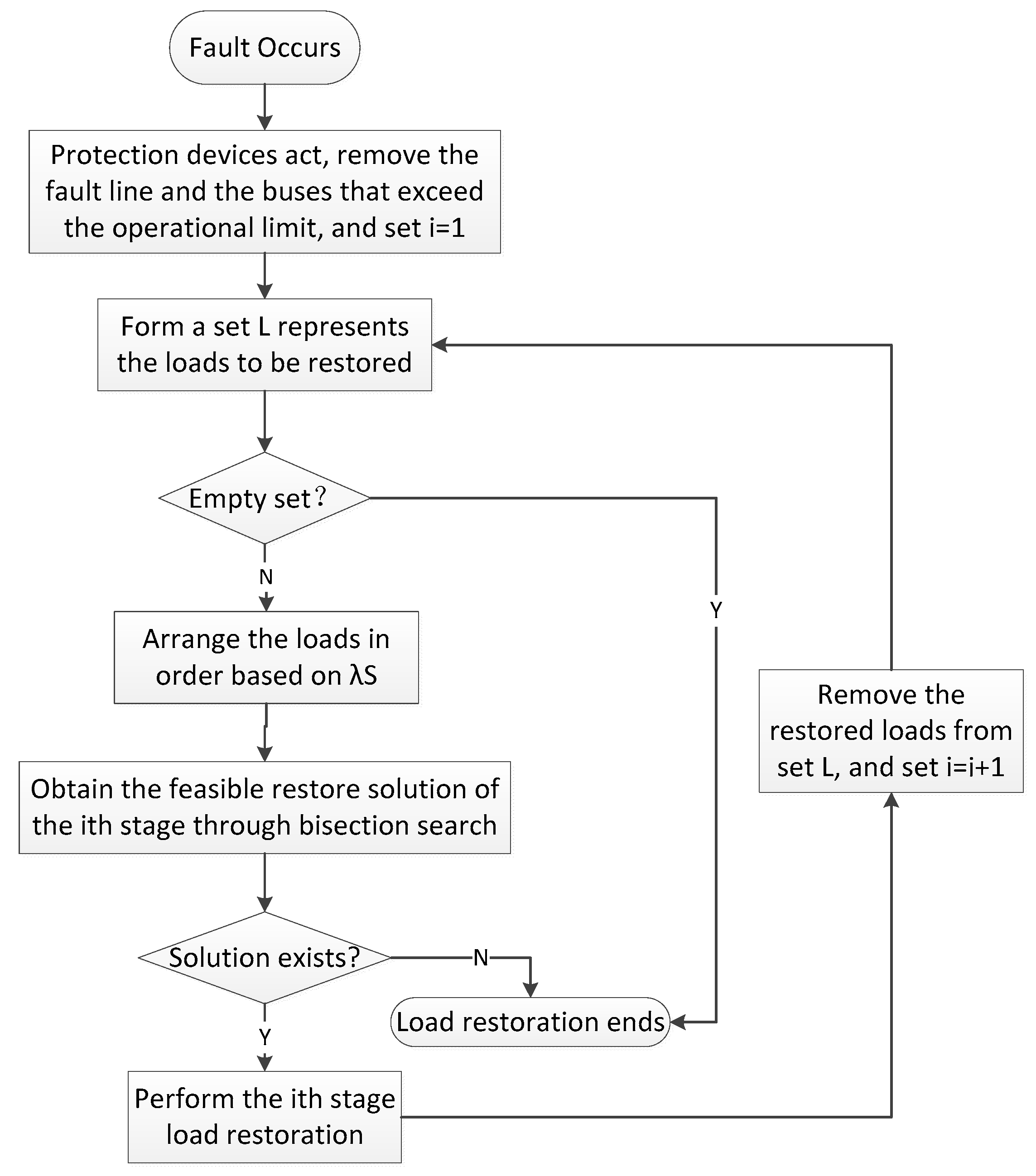
When taking the stability and security constraints into consideration, it is possible that not all the loads can be restored at the same time due to the violation of the constraints. Therefore, the restoration can be divided into several stages, with each stage restoring a portion of unserved loads. The time interval between two stages depends on the dynamic response of the system. Namely, the (i + 1)th stage begin to restore load only when the system tends to be stable after the ith stage restoration. Since the flexible stability and security criterion presented in Section 3 contains non-convex constraints, solving the optimization problem in Equation (22) directly is very time-consuming. To reach a fast load restoration, a heuristic approach is proposed to optimize the survivability of the IPS at each restoration stage, and the loads to be restored are arranged in order according to their level of importance and capacity. The flowchart of the proposed heuristic approach is depicted in Figure 2, and detailed steps are described in the following paragraphs.
Step 0. The IPS is influenced by external disturbances, and fault occurs.
Step 1. According to the operational limit, failure lines and buses exceed the security limit are removed by protection devices. Set .
Step 2. Form a load set that represents all the outage loads which require to be restored.
Step 3. Check whether the load set is empty. If yes, go to step 8. Otherwise, go to the next step.
Step 4. Arrange the loads in order based on their level of importance and capacity.
Step 5. The ith stage restoration strategy is obtained through a bisection search over the loads to be restored, and the feasibility of restoration is checked by the criterion presented in Section 3.
Step 6. Check whether the restoration strategy obtained at the ith stage is feasible. If no, go to step 8. Otherwise, go to the next step.
Step 7. Perform restoration strategy at the ith stage obtained from step 6 and remove the restored loads from the load set . After the system status becomes stable, go back to step 2, and then start (i + 1)th stage restoration. Set .
Step 8. The end of the load restoration process.
4.2. Bisection Search for the ith-Stage Restoration
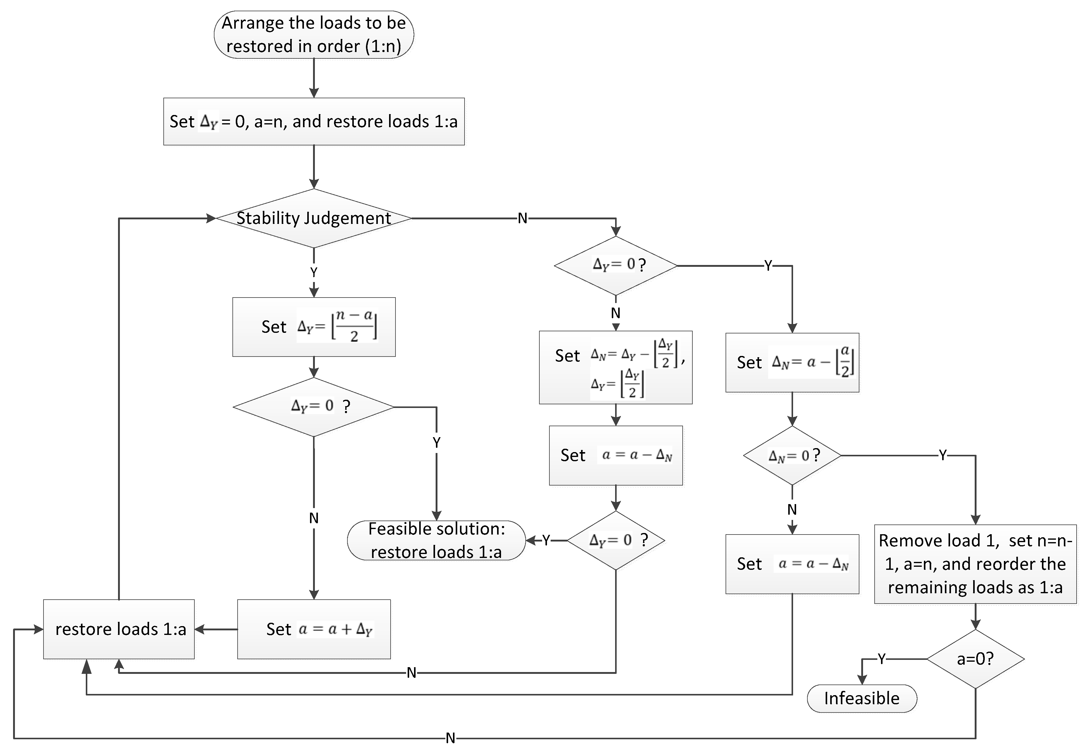
In the heuristic approach proposed in Section 4.1, the restoration strategy at each stage is calculated through a bisection search over the load set . The bisection searching method is proposed in this section, the process of which is depicted in Figure 3.
Step 0. Arrange all the loads that need to be restored in order (1:n), as shown in Section 4.1. Where n denotes the number of loads that need to be restored.
Step 1. Set , where denotes the stability index of the stability judgement. Set , and the loads to be restored are represented as load .
Step 2. Run stability and security analysis based on the criterion presented in Section 3. Check whether the system states are within the security operational limits when loads are restored. If yes, go to the next step. Otherwise go to step 7.
Step 3. Set the stability index , where denotes rounding down a number to the largest integer, namely is the largest integer that does not exceed .
Step 4. Whether the stability index equals 0. If yes, go to step 11. Otherwise, go to the next step.
Step 5. Set .
Step 6. The loads to be restored next are denoted by loads , and go back to step 2.
Step 7. Whether the stability index equals to 0. If yes, go to step 12. Otherwise, go to the next step.
Step 8. Set , where denotes the instability index of the stability judgement. In addition, set .
Step 9. Set .
Step 10. Check whether the stability index equals 0. If yes, go to the next step. Otherwise, go back to step 6.
Step 11. Obtain the feasible solution of the ith stage load restoration, and the result is to restore loads .
Step 12. Set the instability index .
Step 13. Whether the instability index equals to 0. If yes, go to step 15. Otherwise, go to the next step.
Step 14. Set , and go back to step 6.
Step 15. Remove the first load in the load set (). Set, , and reorder the remaining loads as .
Step 16. Whether equals to 0. If yes, go to step 17. Otherwise, go back to step 6.
Step 17. The iteration ends, and the ith stage restoration is infeasible.
5. Case Study
In this section, an IPS with a structure constructed based on the IEEE 14 bus system is used as an example. The IPS consists of 5 generators (), 9 induction motors () and 2 constant impedance loads () as depicted in Figure 4. The mathematical model of generators and induction motors are presented in Appendix A, and the corresponding parameters are shown in Appendix B. The voltage dynamics of a generator are described as a fourth order model, and the induction motor is modeled by a third order electro-mechanical transient model, which can be found in [10]. Transient simulations are conducted on PSCAD/EMTDC (version 4.2.1, Manitoba HVDC Research Centre, Winnipeg, MB, Canada), which are performed to verify the effectiveness of the proposed method.
5.1. Load Restoration Test
Table 1 presents the importance level as well as the nominal capacities of the loads in the system. Based on the heuristic approach proposed in Section 4, the set of loads to be restored is formulated in sequence with respect to the product of importance level and capacity of each load. If the products of some loads are the same, they will be formulated in sequence with respect to the load number. Thus, the corresponding set of loads to be restored is formulated in sequence as during the restoration process.
The power quality [29,30] of IPS should satisfy certain requirements during its normal operation. In this paper, the IPS’s operational limits are selected according to the rules of China Classification Society [31]: (a) bus voltage fluctuations must not exceed ±20% of the nominal voltage during a transient; (b) steady-state bus voltage must not exceed ±5% of the nominal voltage. The operational limits are used to estimate the local region of external inputs of subsystems. The asymptotic gains and local region of inputs of generators, and loads are calculated as shown in Table 2.
The function of generators and induction motors is estimated through the algorithm in [24], and the values of functions are updated based on the initial states of each stage. Assume the transient of the constant impedance load ends very fast, so the functions of constant impedance loads are considered as .
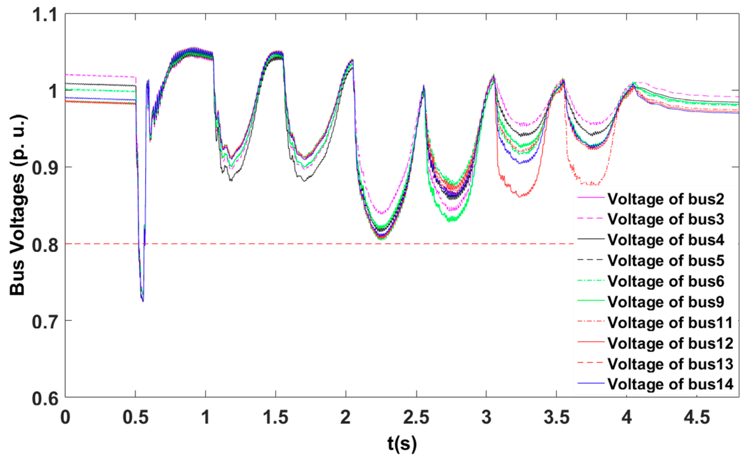
Case 1: A three-phase to ground fault with the ground resistance of is applied at generator bus at s. Bus voltages drop below the operational limits, and the terminal line of is isolated at s with all the loads shed at the same time. The restoration starts from s after the voltage recovers. The time interval of each stage is selected as 0.5 s to ensure the dynamics of the previous restoration ends and the system status is around normal operation point.
By using the algorithm proposed in Section 4, the results of load restoration problem are obtained: . The restoration is divided into 6 stages, and the details of each restoration stage are shown in Table 3. It can be seen that the loads are restored gradually according to the sequence given above. The dynamics of the restored load bus voltages are depicted in Figure 5.
It can be seen from Figure 5 and Table 3 that, during and after the restoration, the dynamics of bus voltages are all within the operational limit. is isolated after the fault, and is tripped due to the capacity constraints. As discussed in the criterion proposed in Section 3, the small gain condition holds during the restoration process, which means that the system dynamics will converge to a certain equilibrium point, while the security is checked through the second condition in the criterion. The left side of the inequality in the security condition shows the supremum norm of input of each device, thus the elements corresponding to load buses indicate the maximum voltage drop of each load bus. As shown in Table 3, the maximum voltage drop occurs at the restored load bus at each restoration stage. It can be seen from Table 3 that the computation of each stage is very fast. It is because in the proposed method, the stability and security criterion inequalities proposed in Section 3 are checked only once for each possible topology of the IPS in restoration, which saves computational time significantly. The proposed heuristic method also accelerates the optimization procedure.
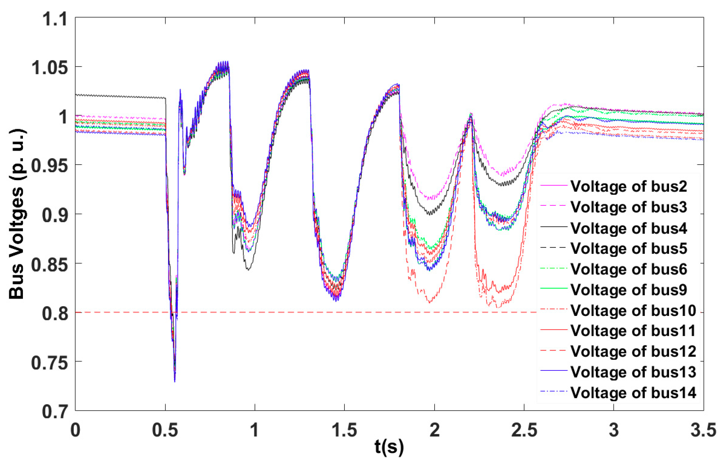
Case 2: A three-phase to ground fault is applied to line 13–14 at s, the corresponding ground resistance is . The fault line is tripped, and all the loads are shed at s since bus voltages drop below the operational limits. The restoration process starts at s.
The obtained load restoration strategy is as follows: . The restoration is divided into 4 stages, and the details of each restoration stage are shown in Table 4. The dynamics of the restored load bus voltages are depicted in Figure 6.
It can be seen from Figure 6 and Table 4 that all the loads are restored by performing a 4-stage restoration. The dynamics of bus voltages are all within the operational limit during and after the restoration. The maximum voltage drop of each restoration stage is estimated through the security constraint proposed in Section 3 and is verified through the simulation results as shown in Figure 6. As shown in Table 4, the calculation time of the restoration is very fast due to the decomposed stability criterion and the proposed heuristic search approach.
The above cases verify the effectiveness of the proposed fast load restoration algorithm. The main benefit of the proposed approach is its ability to consider transient stability and security constraints of the IPS flexibly and fast, which can be analyzed just by checking two algebraic inequalities. By decomposing the dynamic system into several subsystems, it is easier to analyze the stability of each subsystem with a relatively lower dimension. The changes in system topology only have an influence on the relationship of inputs and outputs of subsystems, which reduces computational burden greatly.
5.2. Discussion
The existing research on fast load restoration mainly considers the capacity limits of the IPS, and the restoration strategies are obtained under static constraints. Since the dynamic performance of the system during the restoration process is unconsidered, potential transient stability and security problem may occur in the practical application of the restoration strategies. Compared with the conventional restoration approaches, the proposed approach combines the stability and security constraints through a decomposed stability and security criterion. The restoration process is separated into several stages, the solution of which is obtained with the proposed heuristic method. The solution of the restoration strategy is very fast by checking two algebraic inequalities, and the efficiency can be further improved by applying parallel computing as well as sparse matrix technologies. The proposed fast load restoration approach as well as the ISS-based stability criterion can also be applied to other types of IPS, such as sustainable building [32] and stand-alone hybrid power systems [33], considering stability issues.
6. Conclusions and Future Work
This paper presents a novel idea on the fast restoration of IPS, the major advantage of which is its ability to satisfy transient stability and security requirements of IPS. Based on the ISS theory, the system dynamics are considered in the restoration analytically, which have good adaptability for IPS with flexible topologies. A heuristic approach for load restoration is proposed to solve the optimization problem. The load restoration procedure is divided into several stages, and the feasibility of each restoration stage is checked using bisection search over the loads to be restored. Applications of the proposed method to an IPS consisting of generators, induction motors and constant impedance loads is presented. Transient stability and security of the IPS in the load restoration procedure are verified by time domain simulations.
In this paper, the restoration procedure is separated into several stages with equal time intervals. To achieve a faster restoration strategy, length of the time intervals remains to be optimized. By accurately estimating the IPS’s dynamic response based on the ISS theory, algorithms for reducing the length of the time intervals are needed while guaranteeing the stability of IPS. Further research to extend the proposed method to large-scale power systems is undergoing. A more general LISS/LIOS analysis methodology should be developed to reduce the conservativeness of stability analysis for the application to large systems.
In addition, this paper mainly focused on the IPS with traditional fossil fuel generators, which are usually applied to circumstances such as shipboards and airplanes. Future work is undergoing to apply the proposed algorithm in the restoration of distribution networks with renewable energy sources and microgrids. After an extreme weather event, blackout may occur in the networks due to device failures. In the circumstance, restoration is used to make full use of the available energy storage to supply critical loads and enhance the resilience of the distribution network. Prior work is done in [5], where microgrids are used to restore loads based on the analysis of their ability to supply loads. In [34], pre-hurricane resource allocation is considered which helps to improve the effectiveness of load restoration after a hurricane occurs. In these prior works, the uncertainty of sustainable sources is carefully considered and modeled. The application of the proposed approach in this paper to the resilience enhancement of distribution network considering stability issue is undergoing, and the stability conditions dealing with uncertainties should be addressed through further research.
Acknowledgments
This work was supported by National Natural Science Foundation of China (51707147), Key Research and Development Program of Shaanxi (2017ZDCXL-GY-02-03), State Key Laboratory of Electrical Insulation and Power Equipment (EIPE17313), China Postdoctoral Science Foundation (2017M623171), Shaanxi Postdoctoral Science Foundation (2017BSHEDZZ27), partly supported by Mid-career Researcher Development Program, Faculty of EIT, The University of Sydney, and China Scholarship Council (201706285027).
Author Contributions
Boyu Qin proposed the flexible stability and security criterion, performed the simulations, and wrote the paper. Haixiang Gao proposed the heuristic approach to solve the load restoration problem. Jin Ma proved the flexible criterion, and conducted part of the simulation. Wei Li proposed the load restoration search strategies. Albert Y. Zomaya provided guidance on the problem formulation and case study part.
Conflicts of Interest
The authors declare no conflict of interest.
Appendix A. Models of the Generator and Induction Motor [11]

Table A1.
Implication of generator variables.
| Variable | Implication |
|---|---|
| d-axis synchronous reactance (p.u.) and the transient reactance (p.u.) | |
| the voltage (p.u.) behind and the generator field voltage (p.u.) | |
| the d-axis open circuit transient time constant of the generator | |
| , / | the d-axis and q-axis stator phase currents and voltages |
| , | the output (p.u.) of voltage regulator and the generator bus voltage (p.u.) |
| , | the exciter negative feedback voltage (p.u.) and reference voltage (p.u.) |
| , , , , , | the time constants and gain coefficients of the excitation system |
| saturation coefficient |
Induction motor model:
where the implication of variables is listed in Table A2.
Table A2.
Implication of Induction Motor variables.
| Variable | Implication |
|---|---|
| , , , | slip (p.u.), rotor reactance, transient reactance, and stator resistance |
| , | the real part and the imaginary part (p.u.) of transient voltage |
| , | the real part and the imaginary part (p.u.) of the stator terminal voltage |
| , | the real part and the imaginary part (p.u.) of the stator current |
| , | the rotor circuit time constant and the inertia constant |
| , | the mechanical power and the output active power of the induction motor |
Appendix B. Parameters of the IPS Shown in Figure 4
Reference Value: = , .
Generator: Nominal voltage: , Nominal power: , , , , .
Excitation system: , , , , and , .
Induction motor: Nominal power: , , , . Nominal voltage: . , , , , .
Constant impedance load: (p.u.)
Impedance of transmission line: ,, , .
References
- Concordia, C.; Fink, L.H.; Poullikkas, G. Load Shedding on an Isolated System. IEEE Trans. Power Syst. 1995, 10, 1467–1472. [Google Scholar] [CrossRef]
- Miu, K.N.; Chiang, H.D.; Yuan, B.; Darling, G. Fast service restoration for large-scale distribution systems with priority customers and constraints. IEEE Trans. Power Syst. 1997, 13, 789–795. [Google Scholar] [CrossRef]
- Ramos, E.R.; Martinez-Ramos, J.L.; Exposito, A.G.; Salado, A.J.U. Optimal Reconfiguration of Distribution Networks for Power Loss Reduction. In Proceedings of the 2001 IEEE Porto Power Tech, Porto, Portugal, 10–13 September 2001; Volume 3, p. 5. [Google Scholar]
- Morelato, A.L.; Monticelli, A.J. Heuristic search approach to distribution system restoration. IEEE Trans. Power Deliv. 1989, 4, 2235–2241. [Google Scholar] [CrossRef]
- Gao, H.; Chen, Y.; Xu, Y.; Liu, C.-C. Resilience-Oriented Critical Load Restoration Using Microgrids in Distribution Systems. IEEE Trans. Smart Grid 2016, 7, 2837–2848. [Google Scholar] [CrossRef]
- Leccese, F. Remote-Control System of High Efficiency and Intelligent Street Lighting Using a ZigBee Network of Devices and Sensors. IEEE Trans. Power Deliv. 2013, 28, 21–28. [Google Scholar] [CrossRef]
- Chen, C.S.; Lin, C.H.; Tsai, H.Y. A rule-based expert system with colored petri net models for distribution system service restoration. IEEE Trans. Power Syst. 2002, 17, 1073–1080. [Google Scholar] [CrossRef]
- Nagata, T.; Sasaki, H. An Efficient Algorithm for Distribution Network Restoration. In Proceedings of the 2001 IEEE Power Engineering Society Summer Meeting, Vancouver, BC, Canada, 15–19 July 2001; Volume 1, pp. 54–59. [Google Scholar]
- Hsiao, Y.; Chien, C. Enhancement of restoration service in distribution systems using a combination fuzzy-GA method. IEEE Trans. Power Syst. 2000, 15, 1394–1400. [Google Scholar] [CrossRef]
- Baldwin, T.L.; Lewis, S.A. Distribution load flow methods for shipboard power systems. IEEE Trans. Ind. Appl. 2004, 40, 1183–1190. [Google Scholar] [CrossRef]
- Kundur, P.; Balu, N.J.; Lauby, M.G. Power System Stability and Control; McGraw-Hill: New York, NY, USA, 1994. [Google Scholar]
- Khalil, H.K. Nonlinear Systems, 3rd ed.; Pearson Education: London, UK, 2014. [Google Scholar]
- Pai, M.A. Energy Function Analysis for Power System Stability; Kluwer Academic Press: Dordrecht, The Netherlands, 1989. [Google Scholar]
- Chiang, H.D. Direct Methods for Stability Analysis of Electric Power Systems; Wiley: New York, NY, USA, 2011. [Google Scholar]
- Chiang, H.D.; Hirsch, M.W.; Wu, F.F. Stability regions of nonlinear autonomous dynamical systems. IEEE Trans. Autom. Control 1988, 33, 16–27. [Google Scholar] [CrossRef]
- Li, F.; Chen, Y.; Qin, B.Y.; Shen, C. Decomposed input-output stability analysis and enhancement of integrated power systems. Sci. China Technol. Sci. 2018, 61, 427–437. [Google Scholar] [CrossRef]
- Sontag, E.D. Smooth stabilization implies coprime factorization. IEEE Trans. Autom. Control 1989, 34, 435–443. [Google Scholar] [CrossRef]
- Sontag, E.D.; Wang, Y. New characterizations of input to state stability. IEEE Trans. Autom. Control 1996, 41, 1283–1294. [Google Scholar] [CrossRef]
- Qin, B.; Zhang, X.; Ma, J.; Mei, S. Algorithm for Local Input to State Stability Analysis. IET Control Theory Appl. 2016, 10, 1556–1564. [Google Scholar] [CrossRef]
- Dashkovskiy, S.N.; Rüffer, B.S.; Wirth, F.R. An ISS small-gain theorem for general networks. Math. Control Signals Syst. 2007, 19, 93–122. [Google Scholar] [CrossRef]
- Qin, B.; Zhang, X.; Ma, J.; Deng, S.; Mei, S.; Hill, D.J. Input to State Stability Based Control of Doubly Fed Wind Generator. IEEE Trans. Power Syst. 2017, in press. [Google Scholar] [CrossRef]
- Liu, T.; Hill, D.J.; Jiang, Z.P. Lyapunov formulation of ISS cyclic-small-gain in continuous-time dynamical networks. Automatica 2011, 47, 2088–2093. [Google Scholar] [CrossRef]
- Liu, T.; Jiang, Z.P.; Hill, D.J. Nonlinear Control of Dynamic Networks; CRC Press: Orlando, FL, USA, 2014. [Google Scholar]
- Qin, B.; Zhang, X.; Ma, J.; Mei, S.; Hill, D.J. Local Input to State Stability Based Stability Criterion with Applications to Isolated Power Systems. IEEE Trans. Power Syst. 2016, 31, 5094–5105. [Google Scholar] [CrossRef]
- Kera, K.; Bekki, K.; Osumi, H.; Mori, K. Autonomous Successive Construction Technology without Stopping System Operation for Real-Time System. In Proceedings of the Sixth International Symposium on Autonomous Decentralized Systems, Pisa, Italy, 11 April 2003; pp. 266–273. [Google Scholar]
- Kera, K.; Bekki, K.; Mori, K.; Masumoto, I. High Assurance Step-by-Step Autonomous Construction Technique for Large Real Time System. In Proceedings of the 7th IEEE International Symposium on High Assurance Systems Engineering, Tokyo, Japan, 23–25 October 2002; pp. 79–86. [Google Scholar]
- Sontag, E.D.; Wang, Y. Notions of input to output stability. Syst. Control Lett. 1999, 38, 235–248. [Google Scholar] [CrossRef]
- Lin, Y.; Sontag, E.D.; Wang, Y. A smooth converse Lyapunov theorem for robust stability. SLAM J. Control Optim. 1996, 34, 124–160. [Google Scholar] [CrossRef]
- Masnicki, R. Validation of the Measurement Characteristics in an Instrument for Power Quality Estimation—A Case Study. Energies 2017, 10, 536. [Google Scholar] [CrossRef]
- Leccese, F.; Cagnetti, M.; Pasquale, S.D.; Giarnetti, S.; Caciotta, M. A New Power Quality Instrument Based on Raspberry-Pi. Electronics 2016, 5, 64. [Google Scholar] [CrossRef]
- China Classification Society. Rules for Construction and Classification of Sea-Going High Speed Craft; China Classification Society: Beijing, China, 2015; pp. 1–7. [Google Scholar]
- Sechilariu, M.; Locment, F.; Wang, B. Photovoltaic Electricity for Sustainable Building. Efficiency and Energy Cost Reduction for Isolated DC Microgrid. Energies 2015, 8, 7945–7967. [Google Scholar] [CrossRef]
- Iglesias, F.; Palensky, P.; Cantos, S. Demand Side Management for Stand-Alone Hybrid Power Systems Based on Load Identification. Energies 2012, 5, 4517–4532. [Google Scholar] [CrossRef]
- Gao, H.; Chen, Y.; Mei, S.; Huang, S.; Xu, Y. Resilience-Oriented Pre-Hurricane Resource Allocation in Distribution Systems Considering Electric Buses. Proc. IEEE 2017, 105, 1214–1233. [Google Scholar] [CrossRef]
Figure 1.
Functional models of subsystems.
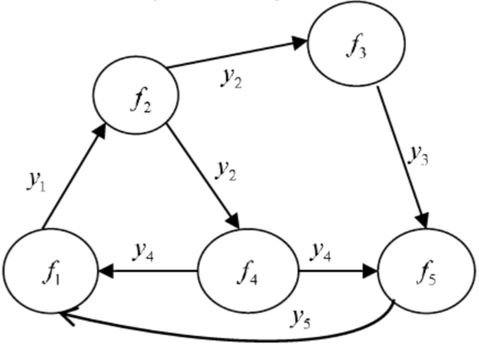
Figure 2.
Flowchart of the heuristic restoration approach.

Figure 3.
Flowchart of the Bisection Search for ith-stage Restoration.

Figure 4.
Configuration of an IPS.
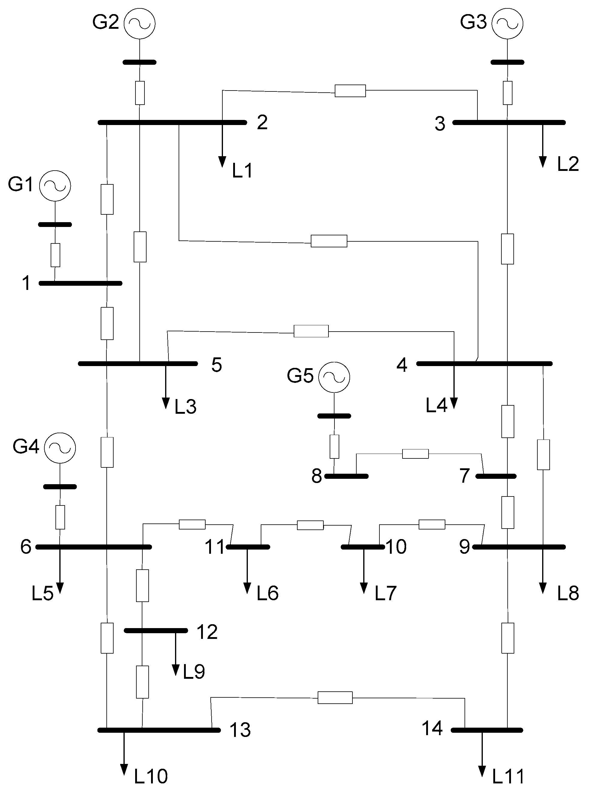
Figure 5.
Dynamics of the bus voltages in Case 1.

Figure 6.
Dynamics of the bus voltages in case 2.

Table 1.
Level of importance of loads.
| Load | |||||
|---|---|---|---|---|---|
| Nominal Power (MVA) | 0.4 | 0.3 | 0.25 | 0.2 | 0.1 |
| Level | Crucial | Vital | Vital | Important | Normal |
| Coefficient () | 4 | 2 | 2 | 1 | 0.5 |
Table 2.
LIOS properties of subsystems.
| Generator | Asymptotic Gain | Local Region of Inputs |
|---|---|---|
| 0.058 | 2.358 | |
| 0.0633 | 2.176 | |
| 7.252 | 0.192 | |
| 5.439 | 0.194 | |
| 4.5325 | 0.195 | |
| 3.626 | 0.195 | |
| 0.4819 | 0.194 |
Table 3.
Restoration process of case 1.
| Stage | Restore Load | Maximum Voltage Drop | Computational Cost | |
|---|---|---|---|---|
| Bus | Voltage Drop (p.u.) | |||
| 1 | 2 | 0.118 | 0.00872 s | |
| 2 | 5 | 0.119 | 0.00896 s | |
| 3 | , | 6 | 0.191 | 0.00711 s |
| 4 | 9 | 0.172 | 0.00948 s | |
| 5 | 12 | 0.139 | 0.00446 s | |
| 6 | , , | 11 | 0.126 | 0.00237 s |
Table 4.
Restoration process of case 2.
| Stage | Restore Load | Maximum Voltage Drop | Computational Cost | |
|---|---|---|---|---|
| Bus | Voltage Drop (p.u.) | |||
| 1 | 5 | 0.158 | 0.00663 s | |
| 2 | 3 | 0.188 | 0.00892 s | |
| 3 | 12 | 0.19 | 0.00884 s | |
| 4 | 10 | 0.194 | 0.000324 s | |
© 2018 by the authors. Licensee MDPI, Basel, Switzerland. This article is an open access article distributed under the terms and conditions of the Creative Commons Attribution (CC BY) license (http://creativecommons.org/licenses/by/4.0/).
Share and Cite
MDPI and ACS Style
Qin, B.; Gao, H.; Ma, J.; Li, W.; Zomaya, A.Y. An Input-to-State Stability-Based Load Restoration Approach for Isolated Power Systems. Energies 2018, 11, 597. https://doi.org/10.3390/en11030597
AMA Style
Qin B, Gao H, Ma J, Li W, Zomaya AY. An Input-to-State Stability-Based Load Restoration Approach for Isolated Power Systems. Energies. 2018; 11(3):597. https://doi.org/10.3390/en11030597
Chicago/Turabian StyleQin, Boyu, Haixiang Gao, Jin Ma, Wei Li, and Albert Y. Zomaya. 2018. "An Input-to-State Stability-Based Load Restoration Approach for Isolated Power Systems" Energies 11, no. 3: 597. https://doi.org/10.3390/en11030597
Note that from the first issue of 2016, this journal uses article numbers instead of page numbers. See further details here.