An Improved Crow Search Algorithm Applied to Energy Problems
by
 , , , and
Primitivo Díaz
1,* ,
,
Marco Pérez-Cisneros
1,*,
Erik Cuevas
1,*, 
Omar Avalos
1,*,
Jorge Gálvez
1,*,
Salvador Hinojosa
2,* and
Daniel Zaldivar
1,* 1
Departamento de Electrónica, Universidad de Guadalajara, CUCEI Av. Revolución 1500, 44430 Guadalajara, Mexico
2
Departamento de Ingeniería del Software e Inteligencia Artificial, Facultad Informática, Universidad Complutense de Madrid, 28040 Madrid, Spain
*
Authors to whom correspondence should be addressed.
Energies 2018, 11(3), 571; https://doi.org/10.3390/en11030571
Submission received: 2 February 2018
/
Revised: 23 February 2018
/
Accepted: 28 February 2018
/
Published: 6 March 2018
Abstract
:The efficient use of energy in electrical systems has become a relevant topic due to its environmental impact. Parameter identification in induction motors and capacitor allocation in distribution networks are two representative problems that have strong implications in the massive use of energy. From an optimization perspective, both problems are considered extremely complex due to their non-linearity, discontinuity, and high multi-modality. These characteristics make difficult to solve them by using standard optimization techniques. On the other hand, metaheuristic methods have been widely used as alternative optimization algorithms to solve complex engineering problems. The Crow Search Algorithm (CSA) is a recent metaheuristic method based on the intelligent group behavior of crows. Although CSA presents interesting characteristics, its search strategy presents great difficulties when it faces high multi-modal formulations. In this paper, an improved version of the CSA method is presented to solve complex optimization problems of energy. In the new algorithm, two features of the original CSA are modified: (I) the awareness probability (AP) and (II) the random perturbation. With such adaptations, the new approach preserves solution diversity and improves the convergence to difficult high multi-modal optima. In order to evaluate its performance, the proposed algorithm has been tested in a set of four optimization problems which involve induction motors and distribution networks. The results demonstrate the high performance of the proposed method when it is compared with other popular approaches.
1. Introduction
The efficient use of energy has attracted the attention in a wide variety of engineering areas due to its environmental consequences. Induction motors and distribution networks are two representative problems that have strong implications in the massive use of energy.
Induction motors are highly used in industries as electromechanical actuators due to advantages such as ruggedness, cheap maintenance, low cost and simple operation. However, the statistics shows that approximately 2/3 of industrial energy is consumed by the induction motors [1,2]. This high rate of consumption has caused the need to improve their efficiency which is highly dependent on the configuration of their internal parameters. The identification of parameters for induction motors represents a challenging process due to their non-linearity. For this reason, the parameter identification of induction motors is currently considered an open research area within the engineering. As a consequence, several algorithms for parameter identification in induction motors have been proposed in the literature [3,4].
On the other hand, distribution networks represent an active research area in electrical systems. The distribution system along with generators and transmission are the three fundamentals components of a power system. Distribution networks are responsible of the loss in the 13% [5,6] of the generated energy. This loss of energy in distribution networks is mainly caused by lack of reactive power in the buses. Capacitor bank allocation in distribution networks have proved to reduce the loss of energy produced by the lack of reactive power. The problem of banks allocation can be formulated as a combinatorial optimization problem where the number of capacitors, their sizes and location have to be optimally selected for satisfying the system restrictions. Many techniques have been proposed to solve this combinatorial optimization problem, which can be classified in four main methods; analytical [5,7,8], numerical [9,10], heuristic [11,12,13], and based on artificial intelligence [14,15]. A detailed study about the methods are described in [15,16,17].
From an optimization perspective, the problems of parameter identification in induction motors and capacitor allocation in distribution networks are considered extremely complex due to their non-linearity, discontinuity, and high multi-modality. These characteristics make difficult to solve them by using standard optimization techniques.
Metaheuristics techniques inspired by the nature have been widely used in recent years to solve many complex engineering problems with interesting results. These methods do not need continuity, convexity, differentiability or certain initial conditions, which represents an advantage over traditional techniques. Particularity parameter identification of induction motors and the capacitor allocation represent two important problems that can be translated as optimization tasks. They have been already faced by using metaheuristic techniques. Some examples include the gravitational search algorithm [18,19], bacterial foraging [20,21], crow search algorithm [14], particle swarm optimization [22,23,24,25], genetic algorithm [26,27], differential evolution [28,29,30], tabu search [31] and firefly [32].
The Crow Search Algorithm (CSA) [33] is a metaheuristic method where individuals emulates the intelligent behavior in a group of crows. Its published results demonstrate its capacity to solve several complex engineering optimization problems. Some examples include its application to image processing [34] and water resources [35]. In spite of its interesting results, its search strategy presents great difficulties when it faces high multi-modal formulations.
In this paper, an enhanced version of the CSA method is proposed to solve the high multi-modal problems of parameter identification in induction motors and capacitor allocation in distribution networks. In the new algorithm, called Improved Crow Search Algorithm (ICSA), two features of the original CSA are modified: (I) the awareness probability (AP) and (II) the random perturbation. With the purpose to enhance the exploration–exploitation ratio the fixed awareness probability (AP) value is replaced (I) by a dynamic awareness probability (DAP), which is adjusted according to the fitness value of each candidate solution. The Lévy flight movement is also incorporated to enhance the search capacities of the original random perturbation (II) of CSA. With such adaptations, the new approach preserves solution diversity and improves the convergence to difficult high multi-modal optima. To evaluate the potential of the proposed method a series of experiments are conducted. In one set of problems, the algorithm is applied to estimate the parameters of two models of induction motors. The other set, the proposed approach is tested in the 10-bus, 33-bus and 64-bus of distribution networks. The results obtained in the experiments are analyzed statistically and compared with related approaches.
The organization of the paper is as follows: Section 2 describes the original CSA, Section 3 the proposed ICSA is presented, Section 4 the motor parameter estimation problem is exposed, Section 5 the capacitor allocation problem is described and Section 6 present the experimental results. Finally, the conclusions are stated in Section 7.
2. Crow Search Algorithm (CSA)
In this section, a general description of the standard CSA is presented. Crow search algorithm is a recent metaheuristic algorithm developed by Askarzadeh [33], which is inspired on the intelligence behavior of crows. In nature, crows evidence intelligence behaviors like self-awareness, using tools, recognizing faces, warn the flock of potentially unfriendly ones, sophisticated communication ways and recalling the food’s hidden place after a while. All these conducts linked to the fact that the brain-body ratio of the crows is slightly lower than the human brain have made it recognized as one of the most intelligent birds in nature [36,37].
The CSA evolutionary process emulates the behavior conducted by crows of hiding and recovering the extra food. As an algorithm based on population, the size of the flock is conformed by N individuals (crows) which are of n-dimensional with n as the problem dimension. The position Xi,k of the crow i in a certain iteration k is described in Equation (1) and represents a possible solution for the problem:
where max Iter is the maximum of iterations in the process. Each crow (individual) is assumed to have the capability of remember the best visited location Mi,k to hide food until the current iteration Equation (2):
The position of each is modified according to two behaviors: Pursuit and evasion.
Pursuit: A crow j follows crow i with the purpose to discover its hidden place. The crow i does not notice the presence of the other crow, as consequence the purpose of crow j is achieve.
Evasion: The crow i knows about the presence of crow j and in order to protect its food, crow i intentionally take a random trajectory. This behavior is simulated in CSA through the implementation of a random movement.
The type of behavior considered by each crow i is determinate by an awareness probability (AP). Therefore, a random value ri uniformly distributed between 0 and 1 is sampled. If ri is greater or equal than AP, behavior 1 is applied, otherwise situation two is chosen. This operation can be summarized in the following model:
The flight length fli,k parameter indicates the magnitude of movement from crow Xi,k towards the best position Mj,k of crow j, the ri is a random number with uniform distribution in the range [0, 1].
Once the crows are modified, their position is evaluated and the memory vector is updated as follows:
where the F(·) represents the objective function to be minimized.
3. The Proposed Improved Crow Search Algorithm (ICSA)
The CSA has demonstrated its potential to find the optimum solution for certain search spaces configurations [14,33,38]. However, its convergence is not guaranteed due to the ineffective exploration of its search strategy. Under this condition, its search strategy presents great difficulties when it faces high multi-modal formulations. In the original CSA method, two different elements are mainly responsible of the search process: The awareness probability (AP) and the random movement (evasion). The value of AP is the responsible of provide the balance between diversification and intensification. On the other hand, the random movement directly affects the exploration process through the re-initialization of candidate solutions. In the proposed ICSA method, both elements, the awareness probability (AP) and the random movement, are reformulated.
3.1. Dynamic Awareness Probability (DAP)
The parameter AP is chosen at the beginning of the original CSA method and remains fixed during the optimization process. This fact is not favorable to the diversification–intensification ratio. In order to improve this relation, the awareness probability (AP) is substituted by a dynamic awareness probability (DAP), which is a probability value adjusted by the fitness quality of each candidate solution. The use of probability parameters based on fitness values has been successfully adopted in the evolutionary literature [39]. Therefore, the dynamic awareness probability (DAP) is computed as follows:
where wV represents the worst fitness value seen so-far. Assuming a minimization problem, this value is calculated as follows wV = max(F(Xj,k)). Under this probabilistic approach, promising solutions will have a high probability to be exploited. On the other hand, solutions of bad quality will have a high probability to be re-initialized with a random position.
3.2. Random Movement—Lévy Flight
The original CSA emulates two different behaviors of crows: pursuit and evasion. The behavior of evasion is simulated by the implementation of a random movement which is computed through a random value uniformly distributed.
In nature, the use of strategies to find food is essential to survive. A search method that is not able to explore good sources of food may be fatal for the animal. Lévy flights, introduced by Paul Lévy in 1937, is a type of random walk which has been observed in many species as a foraging pattern [40,41,42]. In Lévy flights, the step size is controlled by a heavy-tailed probability distribution usually known as Lévy distribution. The Lévy Flights are more efficient exploring the search space than the uniform random distribution [43].
In the proposed ICSA, with the objective to have a better diversification on the search space, Lévy flights are used instead of uniform random movements to simulate the evasion behavior. Therefore, a new random position Xi,k+1 is generated adding to the current position Xi,j the computed Lévy flight L.
To obtain a symmetric Lévy stable distribution for L the Mantegna algorithm [44] is used. Under the Mantegna method, the first stage is to calculate the step size Zi as follows:
where a and b are n-dimensional vectors and β = 3/2. The elements of each vector a and b are sampled from the normal distribution characterized by the following parameters:
where Γ(·) denotes a Gamma distribution. After obtaining the value of Zi, the factor L is calculated by the following model:
where the product implies the element-wise multiplications, Xbest represents the best solution seen so far in terms of the fitness quality. Finally, the new position Xi,k+1 is given by:
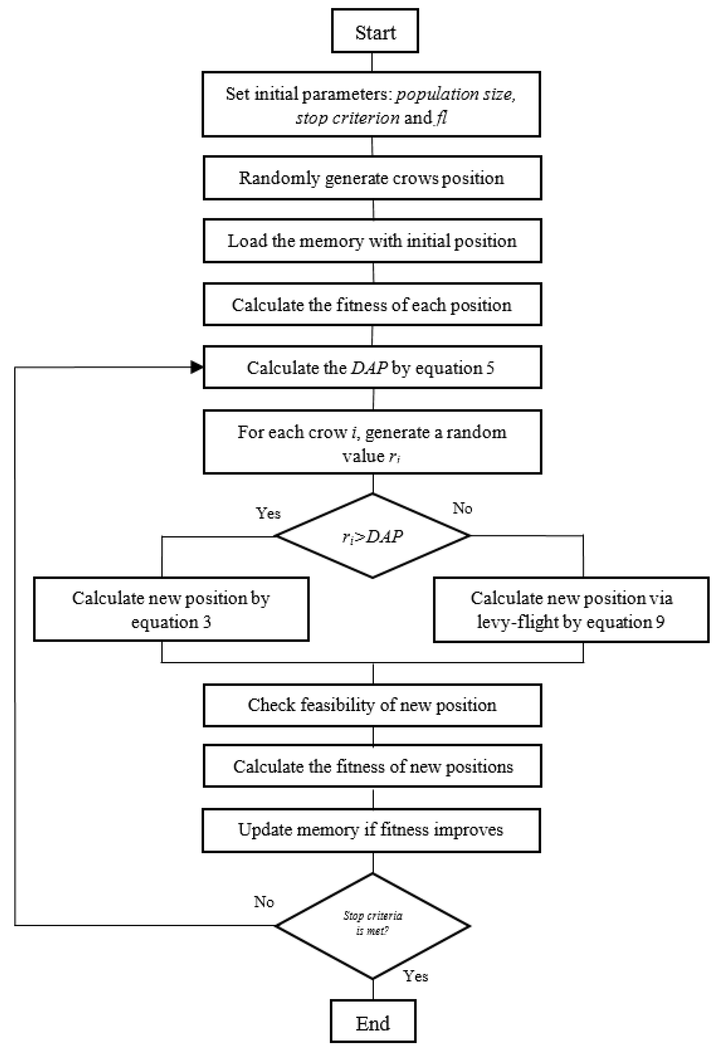
The proposed ICSA algorithm is given in the form of a flowchart in Figure 1.
4. Motor Parameter Estimation Formulation
The physical characteristics of an inductor motor make it complicated to obtain the internal parameter values directly. A way to deal with this disadvantage is estimate them through identification methods. There are two different circuit models that allow a suitable configuration for estimate the motor parameters. The two models are the approximate circuit model and the exact circuit model [4]. The basic difference is the number of parameters included in the model.
The parameter estimation is faced as an n-dimensional optimization problem, where n is the number of internal parameters of the induction motor. The goal is to minimize the error between the estimated parameters and the values provided by the manufacturer, adjusting the parameter values of the equivalent circuit. Under such conditions, the optimization process becomes a challenging task due to the multiple local minima produced with this approach.
4.1. Approximate Circuit Model
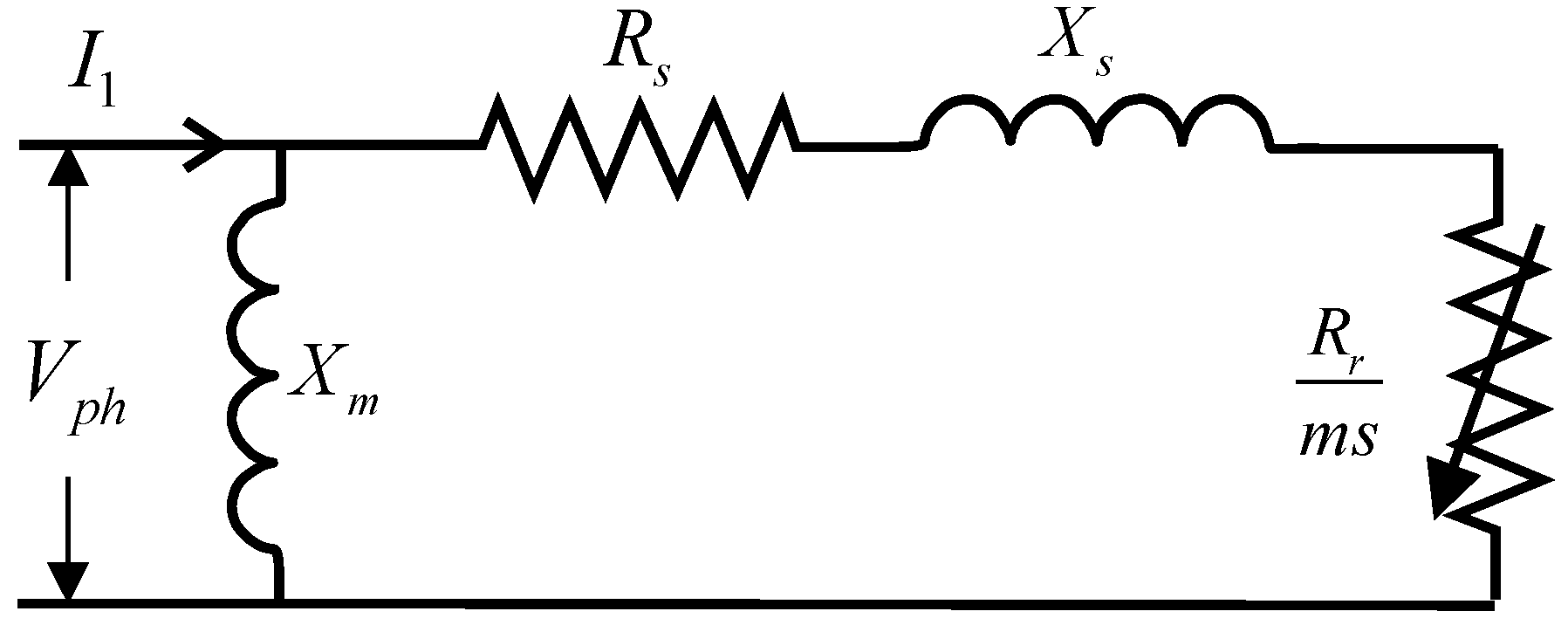
The approximate circuit model characterizes an induction motor without considering the magnetizing and rotor reactance parameters. Thus, the accuracy is less than the exact circuit model.
Figure 2 presents the approximate circuit model. In the Figure, it is represented all the parameters used to characterize the motor such the stator resistance (Rs), rotor resistance (Rr), stator leakage reactance (Xs) and motor slip (ms) which are estimated using the data provided by the manufacture of starting torque (Tstr), maximum torque (Tmax) and full load torque (Tfl). Based on this model, the estimation task can be expressed as the following optimization problem:
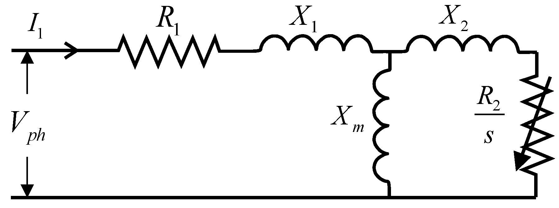
4.2. Exact Circuit Model
Different from the approximate circuit model, the exact circuit model characterizes the induction motor by using all the motor parameters. Figure 3 illustrates the exact circuit model. This circuit configuration includes the parameters stator resistance (Rs), rotor resistance (Rr), stator leakage inductance (Xs) and motor slip (ms) also add two more calculations, the rotor leakage reactance (Xr) and the magnetizing leakage reactance (Xm) to obtain, the maximum torque (Tmax), full load torque (Tfl), starting torque (Tstr) and full load power factor (pf). Based on this exact circuit model, the estimation task can be formulated as the following optimization problem:
where pfl and are the rated power and rotational losses, while nfl is the efficiency given by the manufacturer. The values of pfl and preserve compatibility with related works [3,18]:
5. Capacitor Allocation Problem Formulation
5.1. Load Flow Analysis
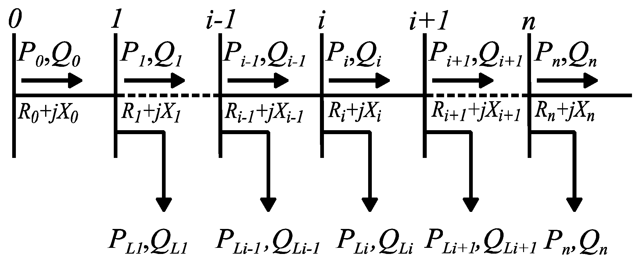
In this section the capacitor allocation problem is described. Therefore, in order to know the characteristics of voltage profile and power losses in a distribution network a load flow analysis is conducted. Several techniques have been considered to accomplish the analysis [45,46]. In this paper, for its simplicity, the method proposed in [47] has been adopted to find the voltages in all buses. Assuming the single line diagram of a three balanced distribution system, as shown in Figure 4, the values of voltage and power losses are calculated as follows:
where is the voltage magnitude in the i-th + 1 node, Ri and Xi are the resistance and the reactance in the branch i. Pi+1 and Qi+1 are the real and reactive power load flowing through node i-th + 1, PLi and QLi are the real and reactive power losses at node i, while PLOSS is the total real loss in the network.
5.2. Mathematical Approach
The optimal allocation of capacitors in distribution network buses is represented by the solution that minimize the annual cost generated by power losses of the whole system (Equation (31)), as well as the cost of capacitor installation (Equation (32)):
where AC is the annual cost generated by the real power losses, kp is the price of losses in kW per year, PLOSS is the total of real power losses in the system, IC represents the installation cost of each capacitor, N corresponds to the number of buses chosen for a capacitor installation, is the cost per kVar, and is the size of capacitor in bus i. The maintenance capacitor cost is not included in the objective function.
Therefore, the general objective function can be expressed as follows:
The minimization of the objective function F is subject to certain voltage constraints given by:
where Vmin = 0.90 p.u. and Vmax = 1.0 p.u. are the lower and upper limits of voltages, respectively. represents the voltage magnitude in bus i.
Under such conditions, in the optimization process, an optimal selection of size, type, number and location of capacitors must be found. This problem is considered a complex optimization task for this reason the proposed ICSA is used to solve it.
5.3. Sensitivity Analysis and Loss Sensitivity Factor
Sensitivity analysis is a technique applied mainly to reduce the search space. The idea is to provide knowledge about the parameters in order to lessen the optimization process. In capacitor allocation problem, the sensitivity analysis is used to obtain the parameters with less variability [48]. This information allows to know the nodes that can be considered as potential candidates to allocate a capacitor. Under such conditions, the search space can be reduced. In addition, the nodes identified with less variability correspond to those which will have greater loss reduction with the capacitor installation.
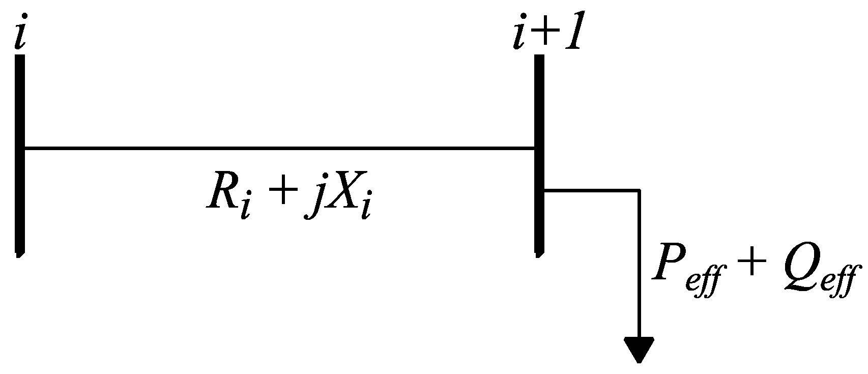
Assuming a simple distribution line from Figure 4, as is shown in Figure 5, the equations of active power loss and reactive power loss (Equations (28)–(29)) can be rewritten as follows:
where the term Peff(i + 1) correspond to the total effective active power presented further the node i + 1, and Qeff(i + 1) is equivalent to the effective value of reactive power supplied further the node i + 1.
Therefore, the loss sensitivity factors now can be obtained from Equations (35) and (36) as follows:
Now, the processes to detect the possible candidate nodes is summarized in the next steps:
- Step 1.
- Using Equation (25) to compute the Loss Sensitivity Factors for all nodes.
- Step 2.
- Sort in descending order the Loss Sensitivity Factors and its corresponding node index.
- Step 3.
- Calculate the normalized voltage magnitudes for all nodes using:
- Step 4.
- Set a node as possible candidate those nodes whose norm value (calculated in the previous step) is less than 1.01.
6. Experiments
In order to evaluate the proposed method, a set of experiments are conducted considering two energy problems. The first experiment is the internal parameter estimation of two induction motor models. The second experiment is implemented over three distribution networks where the objective is to obtain the optimal capacitor allocation for reducing the power losses and improving the voltage profile. The experiments have been executed on a Pentium dual-core computer with a 2.53 GHz CPU and 8-GB RAM.
6.1. Motor Parameter Estimation Test
The performance of the proposed ICSA is tested over two induction motors with the purpose to estimate their optimal parameters. In the experimental process, the approximate and exact circuit model are used. The manufacturer characteristics of the motors are presented in Table 1.
In the test, the results of the proposed ICSA method is compared to those presented by the popular algorithms DE, ABC and GSA. The parameters setting of the algorithms has been used in order to maintain compatibility with other works reported in the literature [18,19,28,49] and are shown in Table 2.
The tuning parameter FL in the ICSA algorithm is selected as result of a sensitivity analysis which through experimentally way evidence the best parameter response. Table 3 shows the sensitivity analysis of the two energy problems treated in this work.
In the comparison, the algorithms are tested with a population size of 25 individuals, with a maximum number of generations established in 3000. This termination criterion as well as the parameter setting of algorithms has been used to maintain concordance with the literature [18,28,49]. Additionally, the results are analyzed and validated statistically through the Wilcoxon test.
The results for the approximate model produced by motor 1 and motor 2 are presented in Table 4 and Table 5, respectively. In the case of exact model the values of standard deviation and mean for the algorithms are shown in Table 6 for motor 1 and the results for motor 2 in Table 7. The results presented are based on an analysis of 35 independent executions for each algorithm. The results demonstrate that the proposed ICSA method is better than its competitors in terms of accuracy (Mean) and robustness (Std.).
The comparison of the final fitness values of different approaches is not enough to validate a new proposal. Other additional test also represents the convergence graphs. They show the evolution of the solutions through the optimization process. Therefore, they indicate which approaches reach faster the optimal solutions. Figure 6 shows the convergence comparison between the algorithms in logarithmic scale for a better appreciation, being the proposed method which present a faster to achieve the global optimal.
6.2. Capacitor Allocation Test
With the purpose to prove the performance of the proposed method a set of three distribution networks, the 10-bus [50], 33-bus [51], and 69-bus [52] is used in this experiment.
In the experiments, the algorithms DE, ABC, GSA has been used for comparison. Their setting parameters are shown in Table 2. For all algorithms the number of search agents and the maximum number of iterations is 25 and 100.
6.2.1. 10-Bus System
The first distribution network comprises a 10-bus system with nine lines. This bus, shown in Figure 7, is considered as a substation bus. Table A1 in the Appendix A shows the system specifications of resistance and reactance of each line, as well as the real and reactive loads for each bus. The system presents a total active and reactive power load of 12,368 kW and 4186 kVAr, while the voltage supplied by the substation is 23 kV.
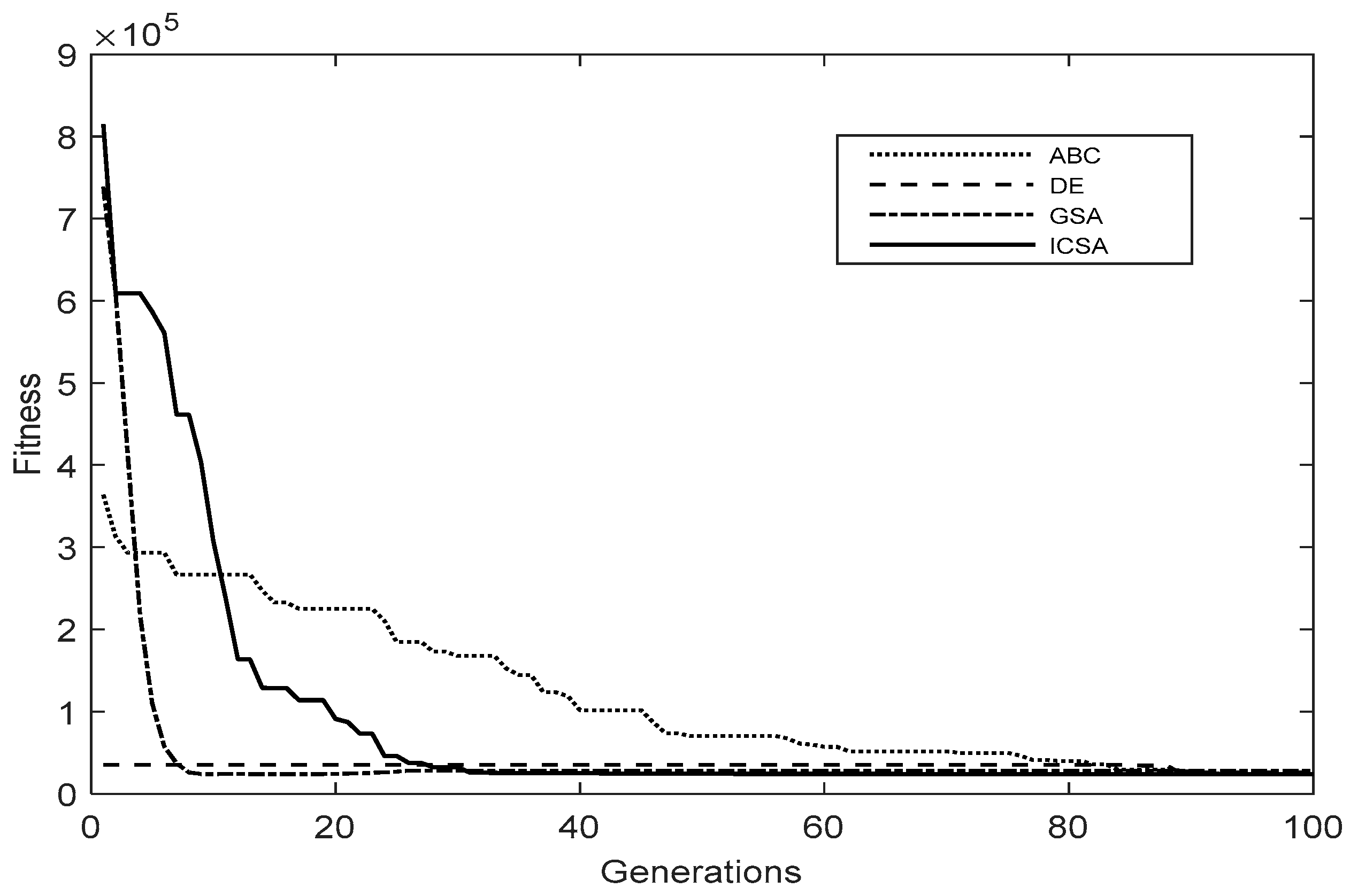
The network in uncompensated mode i.e., before allocating any capacitor, has a total power loss of 783.77 kW, the minimum voltage is 0.8404 p.u. located at 10th bus and the maximum is 0.9930 p.u. at 2nd bus. The cost per kW lost for this experiment and the remainders is $168 with a loss of 783.77 kW, while the annual cost is $131,674. At beginning of the methodology, the sensitivity analysis is used to identify the candidate nodes with a high probability to install a capacitor. In case of the 10-bus, the buses 6, 5, 9, 10, 8 and 7 are considered as candidates. Based on a set of 27 standard capacitor sizes and their corresponding annual price per KVAr, Table 8 shows the capacitor installation in each candidate node obtained by ICSA. After the optimization process the corresponding capacitor sizes are 1200, 3900, 150, 600, 450 kVAr installed in the optimal buses 6, 5, 9, 10, 8. The total power loss is 696.76 kW with an annual cost of $117,055.68. The comparison results obtained by the algorithms are shown in Table 9. Figure 8 illustrates the convergence evolution of the all algorithms.
CSA vs. ICSA
In order to compare directly the original CSA version with the proposed ICSA, the same experiments conducted in [14] have been considered. In the first experiment, the optimization process involves only the candidate buses of 5, 6 and 10 for capacitor allocation. The second test considers all the buses as possible candidates (except the substation bus) for capacitor installation. For the first experiment, all the possible capacitor combinations are (27 + 1)3 = 21952. Under such conditions, it is possible to conduct a brute-force search for obtaining the global best. For this test, both algorithms (CSA and ICSA) have been able to achieve the global minimum.
In the second experiment, all buses are candidates for capacitor allocation. Under this approach, there are (27 + 1)9 = 1.0578 × 10¹³ different combinations. In this scenario, a brute-force strategy is computationally expensive. The results of these experiments are shown in Table 10.
6.2.2. 33-Bus System
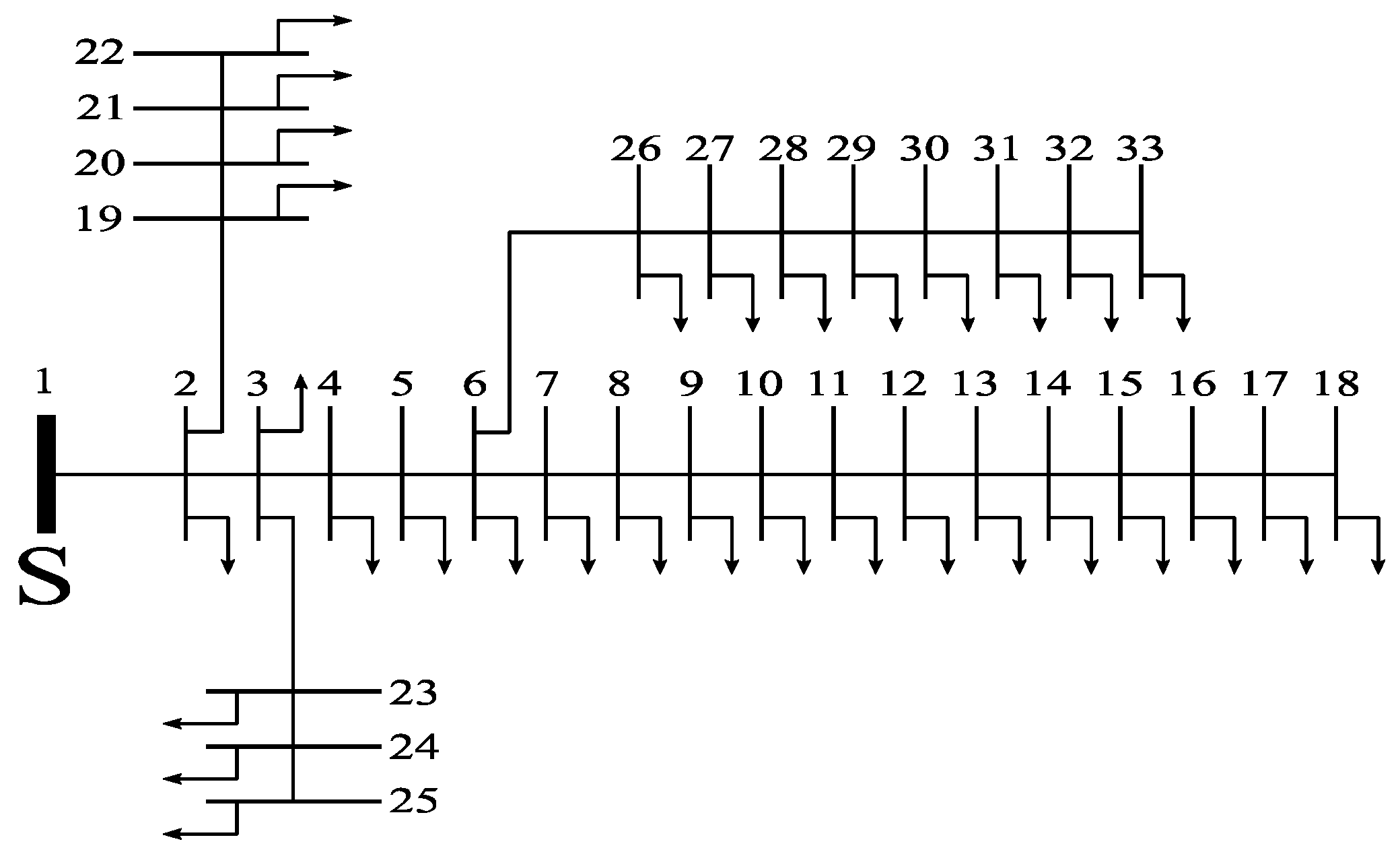
In this experiment, a system with 33 buses and 32 lines is considered. In the system, the first bus is assumed as substation bus with a voltage of 12.66 kV. The network configuration is illustrated in Figure 9.
The information about line resistance and reactance, as well as the corresponding load profile is shown in the Appendix A in Table A2. The 33-bus distribution network before the capacitor installation presents a total power loss of 210.97 kW with an annual cost of $35,442.96 and a total active power of 3715 kW.
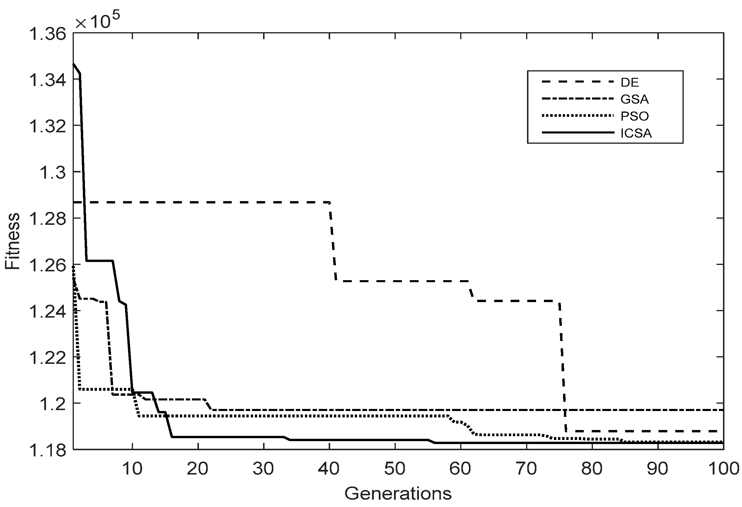
Once the optimization process is conducted, the buses 6, 30, 13 are selected as the optimal location with the corresponding sizes of 450, 900, 350 kVAr. The candidate buses are determined by the sensitivity analysis. The total power loss after the capacitor installation is decreased from 210.91 to 138.74 kW, saving 32.59% of the original cost. The results of the test in detail and the comparison between the algorithms are shown in Table 11. Figure 10 illustrates the convergence evolution of the all algorithms.
CSA vs. ICSA
This section presents a direct comparison between original crow search algorithm (CSA) and the proposed method (ICSA). The 33-bus network is analyzed by CSA as is presented in [14] where the buses 11, 24, 30 and 33 are taken as candidates and the capacitor sizes and their kVar values are shown in Table 12.
The results obtained from the both algorithms are compared in Table 13. The table shows that the ICSA is capable to obtain accurate results than the original version CSA.
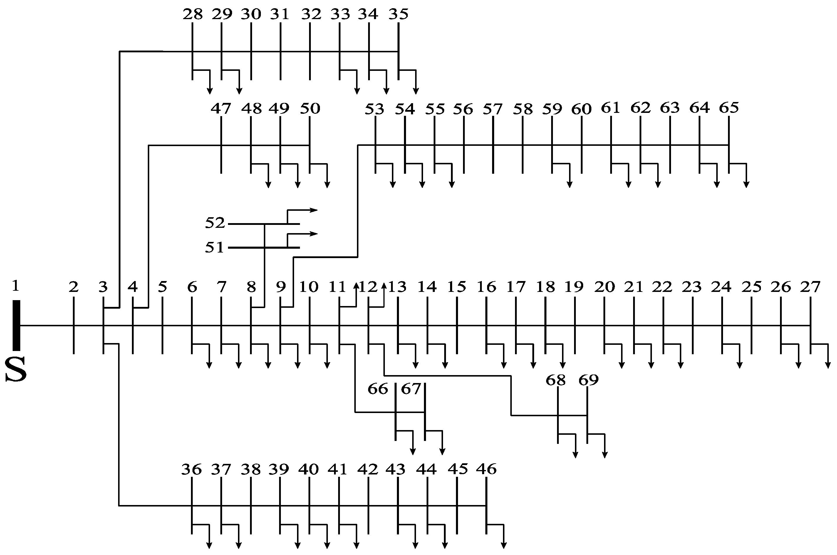
6.2.3. 69-Bus System
For the third capacitor allocation experiment a network of 68 buses and 69 lines is analyzed. Before to install any capacitor, the network presents a total active power loss of 225 kW, a total active and reactive power load of 3801.89 kW and 2693.60 kVAr. The annual cost for the corresponding 225 kW power loss is $37,800.00. The system presents a minimum voltage of 0.9091 p.u. at the 64th bus and a maximum 0.9999 p.u. at 2nd bus. As in the 10 and 33 bus experiments, the possible capacitor sizes and the price per kVAr is shown in the Table 8. The network diagram is illustrated in Figure 11 and the line and load data is presented in Table A3 in the Appendix A.
Using the ICSA method, optimal buses selected are the 57, 61 and 18 with the capacitor values of 150, 1200, 350 kVAr respectively. With this reactance adjustment the total power loss is reduced from 225 to 146.20 kW, saving 33.96% from the original cost. The voltage profile presents a minimum of 0.9313 p.u. at bus 65th and a maximum of 0.9999 2nd. Table 14 shows a detailed comparison between the results obtained by the proposed method and the results of the DE, ABC and GSA algorithms.
6.2.4. Statistical Analysis
In order to validate the results a statistical analysis between the different methods is performed and the results are illustrated in Table 15.
7. Conclusions
In this paper, an improved version of the CSA method is presented to solve complex high multi-modal optimization problems of energy: Identification of induction motors and capacitor allocation in distribution networks. In the new algorithm, two features of the original CSA are modified: (I) the awareness probability (AP) and (II) the random perturbation. With the purpose to enhance the exploration–exploitation ratio the fixed awareness probability (AP) value is replaced (I) by a dynamic awareness probability (DAP), which is adjusted according to the fitness value of each candidate solution. The Lévy flight movement is also incorporated to enhance the search capacities of the original random perturbation (II) of CSA. With such adaptations, the new approach preserves solution diversity and improves the convergence to difficult high multi-modal optima.
In order to evaluate its performance, the proposed algorithm has been compared with other popular search algorithms such as the DE, ABC and GSA. The results demonstrate the high performance of the proposed method in terms of accuracy and robustness.
Author Contributions
Primitivo Díaz and Erik Cuevas wrote the paper. Primitivo Díaz and Omar Avalos proposed the methodology and designed the experiments to implement. Jorge Gálvez and Salvador Hinojosa performed the experiments. Marco Pérez-Cisneros and Daniel Zaldivar analyzed the results of the experiments.
Conflicts of Interest
The authors declare no conflict of interest.
Appendix A. Systems Data

Table A1.
10-bus test system data.
| Line No. | From Bus i | To Bus i + 1 | R (Ω) | X (Ω) | PL (kW) | QL (kVAR) |
|---|---|---|---|---|---|---|
| 1 | 1 | 2 | 1.35309 | 1.3235 | 1840 | 460 |
| 2 | 2 | 3 | 1.17024 | 1.1446 | 980 | 340 |
| 3 | 3 | 4 | 0.84111 | 0.8227 | 1790 | 446 |
| 4 | 4 | 5 | 1.52348 | 1.0276 | 1598 | 1840 |
| 5 | 2 | 9 | 2.01317 | 1.3579 | 1610 | 600 |
| 6 | 9 | 10 | 1.68671 | 1.1377 | 780 | 110 |
| 7 | 2 | 6 | 2.55727 | 1.7249 | 1150 | 60 |
| 8 | 6 | 7 | 1.0882 | 0.7340 | 980 | 130 |
| 9 | 6 | 8 | 1.25143 | 0.8441 | 1640 | 200 |
Table A2.
33-bus test system data.
| Line No. | From Bus i | To Bus i + 1 | R (Ω) | X (Ω) | PL (kW) | QL (kVAR) |
|---|---|---|---|---|---|---|
| 1 | 1 | 2 | 0.0922 | 0.0477 | 100 | 60 |
| 2 | 2 | 3 | 0.4930 | 0.2511 | 90 | 40 |
| 3 | 3 | 4 | 0.3660 | 0.1864 | 120 | 80 |
| 4 | 4 | 5 | 0.3811 | 0.1941 | 60 | 30 |
| 5 | 5 | 6 | 0.8190 | 0.7070 | 60 | 20 |
| 6 | 6 | 7 | 0.1872 | 0.6188 | 200 | 100 |
| 7 | 7 | 8 | 1.7114 | 1.2351 | 200 | 100 |
| 8 | 8 | 9 | 1.0300 | 0.7400 | 60 | 20 |
| 9 | 9 | 10 | 1.0400 | 0.7400 | 60 | 20 |
| 10 | 10 | 11 | 0.1966 | 0.0650 | 45 | 30 |
| 11 | 11 | 12 | 0.3744 | 0.1238 | 60 | 35 |
| 12 | 12 | 13 | 1.4680 | 1.1550 | 60 | 35 |
| 13 | 13 | 14 | 0.5416 | 0.7129 | 120 | 80 |
| 14 | 14 | 15 | 0.5910 | 0.5260 | 60 | 10 |
| 15 | 15 | 16 | 0.7463 | 0.5450 | 60 | 20 |
| 16 | 16 | 17 | 1.2890 | 1.7210 | 60 | 20 |
| 17 | 17 | 18 | 0.7320 | 0.5740 | 90 | 40 |
| 18 | 2 | 19 | 0.1640 | 0.1565 | 90 | 40 |
| 19 | 19 | 20 | 1.5042 | 1.3554 | 90 | 40 |
| 20 | 20 | 21 | 0.4095 | 0.4784 | 90 | 40 |
| 21 | 21 | 22 | 0.7089 | 0.9373 | 90 | 40 |
| 22 | 3 | 23 | 0.4512 | 0.3083 | 90 | 50 |
| 23 | 23 | 24 | 0.8980 | 0.7091 | 420 | 200 |
| 24 | 24 | 25 | 0.8960 | 0.7011 | 420 | 200 |
| 25 | 6 | 26 | 0.2030 | 0.1034 | 60 | 25 |
| 26 | 26 | 27 | 0.2842 | 0.1447 | 60 | 25 |
| 27 | 27 | 28 | 1.0590 | 0.9337 | 60 | 20 |
| 28 | 28 | 29 | 0.8042 | 0.7006 | 120 | 70 |
| 29 | 29 | 30 | 0.5075 | 0.2585 | 200 | 600 |
| 30 | 30 | 31 | 0.9744 | 0.9630 | 150 | 70 |
| 31 | 31 | 32 | 0.3105 | 0.3619 | 210 | 100 |
| 32 | 32 | 33 | 0.3410 | 0.5302 | 60 | 40 |
Table A3.
69-bus test system data.
| Line No. | From Bus i | To Bus i + 1 | R (Ω) | X (Ω) | PL (kW) | QL (kVAR) |
|---|---|---|---|---|---|---|
| 1 | 1 | 2 | 0.00050 | 0.0012 | 0.00 | 0.00 |
| 2 | 2 | 3 | 0.00050 | 0.0012 | 0.00 | 0.00 |
| 3 | 3 | 4 | 0.00150 | 0.0036 | 0.00 | 0.00 |
| 4 | 4 | 5 | 0.02510 | 0.0294 | 0.00 | 0.00 |
| 5 | 5 | 6 | 0.36600 | 0.1864 | 2.60 | 2.20 |
| 6 | 6 | 7 | 0.38100 | 0.1941 | 40.40 | 30.00 |
| 7 | 7 | 8 | 0.09220 | 0.0470 | 75.00 | 54.00 |
| 8 | 8 | 9 | 0.04930 | 0.0251 | 30.00 | 22.00 |
| 9 | 9 | 10 | 0.81900 | 0.2707 | 28.00 | 19.00 |
| 10 | 10 | 11 | 0.18720 | 0.0619 | 145.00 | 104.00 |
| 11 | 11 | 12 | 0.71140 | 0.2351 | 145.00 | 104.00 |
| 12 | 12 | 13 | 1.03000 | 0.3400 | 8.00 | 5.00 |
| 13 | 13 | 14 | 1.04400 | 0.3400 | 8.00 | 5.00 |
| 14 | 14 | 15 | 1.05800 | 0.3496 | 0.00 | 0.00 |
| 15 | 15 | 16 | 0.19660 | 0.0650 | 45.00 | 30.00 |
| 16 | 16 | 17 | 0.37440 | 0.1238 | 60.00 | 35.00 |
| 17 | 17 | 18 | 0.00470 | 0.0016 | 60.00 | 35.00 |
| 18 | 18 | 19 | 0.32760 | 0.1083 | 0.00 | 0.00 |
| 19 | 19 | 20 | 0.21060 | 0.0690 | 1.00 | 0.60 |
| 20 | 20 | 21 | 0.34160 | 0.1129 | 114.00 | 81.00 |
| 21 | 21 | 22 | 0.01400 | 0.0046 | 5.00 | 3.50 |
| 22 | 22 | 23 | 0.15910 | 0.0526 | 0.00 | 0.00 |
| 23 | 23 | 24 | 0.34630 | 0.1145 | 28.00 | 20.00 |
| 24 | 24 | 25 | 0.74880 | 0.2475 | 0.00 | 0.00 |
| 25 | 25 | 26 | 0.30890 | 0.1021 | 14.00 | 10.00 |
| 26 | 26 | 27 | 0.17320 | 0.0572 | 14.00 | 10.00 |
| 27 | 3 | 28 | 0.00440 | 0.0108 | 26.00 | 18.60 |
| 28 | 28 | 29 | 0.06400 | 0.1565 | 26.00 | 18.60 |
| 29 | 29 | 30 | 0.39780 | 0.1315 | 0.00 | 0.00 |
| 30 | 30 | 31 | 0.07020 | 0.0232 | 0.00 | 0.00 |
| 31 | 31 | 32 | 0.35100 | 0.1160 | 0.00 | 0.00 |
| 32 | 32 | 33 | 0.83900 | 0.2816 | 14.00 | 10.00 |
| 33 | 33 | 34 | 1.70800 | 0.5646 | 19.50 | 14.00 |
| 34 | 34 | 35 | 1.47400 | 0.4873 | 6.00 | 4.00 |
| 35 | 3 | 36 | 0.00440 | 0.0108 | 26.00 | 18.55 |
| 36 | 36 | 37 | 0.06400 | 0.1565 | 26.00 | 18.55 |
| 37 | 37 | 38 | 0.10530 | 0.1230 | 0.00 | 0.00 |
| 38 | 38 | 39 | 0.03040 | 0.0355 | 24.00 | 17.00 |
| 39 | 39 | 40 | 0.00180 | 0.0021 | 24.00 | 17.00 |
| 40 | 40 | 41 | 0.72830 | 0.8509 | 1.20 | 1.00 |
| 41 | 41 | 42 | 0.31000 | 0.3623 | 0.00 | 0.00 |
| 42 | 42 | 43 | 0.04100 | 0.0478 | 6.00 | 4.30 |
| 43 | 43 | 44 | 0.00920 | 0.0116 | 0.00 | 0.00 |
| 44 | 44 | 45 | 0.10890 | 0.1373 | 39.22 | 26.30 |
| 45 | 45 | 46 | 0.00090 | 0.0012 | 39.22 | 26.30 |
| 46 | 4 | 47 | 0.00340 | 0.0084 | 0.00 | 0.00 |
| 47 | 47 | 48 | 0.08510 | 0.2083 | 79.00 | 56.40 |
| 48 | 48 | 49 | 0.28980 | 0.7091 | 384.70 | 274.50 |
| 49 | 49 | 50 | 0.08220 | 0.2011 | 384.70 | 274.50 |
| 50 | 8 | 51 | 0.09280 | 0.0473 | 40.50 | 28.30 |
| 51 | 51 | 52 | 0.33190 | 0.1140 | 3.60 | 2.70 |
| 52 | 9 | 53 | 0.17400 | 0.0886 | 4.35 | 3.50 |
| 53 | 53 | 54 | 0.20300 | 0.1034 | 26.40 | 19.00 |
| 54 | 54 | 55 | 0.28420 | 0.1447 | 24.00 | 17.20 |
| 55 | 55 | 56 | 0.28130 | 0.1433 | 0.00 | 0.00 |
| 56 | 56 | 57 | 1.59000 | 0.5337 | 0.00 | 0.00 |
| 57 | 57 | 58 | 0.78370 | 0.2630 | 0.00 | 0.00 |
| 58 | 58 | 59 | 0.30420 | 0.1006 | 100.00 | 72.00 |
| 59 | 59 | 60 | 0.38610 | 0.1172 | 0.00 | 0.00 |
| 60 | 60 | 61 | 0.50750 | 0.2585 | 1244.00 | 888.00 |
| 61 | 61 | 62 | 0.09740 | 0.0496 | 32.00 | 23.00 |
| 62 | 62 | 63 | 0.14500 | 0.0738 | 0.00 | 0.00 |
| 63 | 63 | 64 | 0.71050 | 0.3619 | 227.00 | 162.00 |
| 64 | 64 | 65 | 1.04100 | 0.5302 | 59.00 | 42.00 |
| 65 | 11 | 66 | 0.20120 | 0.0611 | 18.00 | 13.00 |
| 66 | 66 | 67 | 0.00470 | 0.0014 | 18.00 | 13.00 |
| 67 | 12 | 68 | 0.73940 | 0.2444 | 28.00 | 20.00 |
| 68 | 68 | 69 | 0.00470 | 0.0016 | 28.00 | 20.00 |
References
- Prakash, V.; Baskar, S.; Sivakumar, S.; Krishna, K.S. A novel efficiency improvement measure in three-phase induction motors, its conservation potential and economic analysis. Energy Sustain. Dev. 2008, 12, 78–87. [Google Scholar] [CrossRef]
- Saidur, R. A review on electrical motors energy use and energy savings. Renew. Sustain. Energy Rev. 2010, 14, 877–898. [Google Scholar] [CrossRef]
- Perez, I.; Gomez-Gonzalez, M.; Jurado, F. Estimation of induction motor parameters using shuffled frog-leaping algorithm. Electr. Eng. 2013, 95, 267–275. [Google Scholar] [CrossRef]
- Sakthivel, V.P.; Bhuvaneswari, R.; Subramanian, S. Artificial immune system for parameter estimation of induction motor. Expert Syst. Appl. 2010, 37, 6109–6115. [Google Scholar] [CrossRef]
- Lee, S.; Grainger, J. Optimum Placement of Fixed and Switched Capacitors on Primary Distribution Feeders. IEEE Trans. Power Appar. Syst. 1981, 345–352. [Google Scholar] [CrossRef]
- Zidar, M.; Georgilakis, P.S.; Hatziargyriou, N.D.; Capuder, T.; Škrlec, D. Review of energy storage allocation in power distribution networks: Applications, methods and future research. IET Gener. Transm. Distrib. 2016, 3, 645–652. [Google Scholar] [CrossRef]
- Grainger, J.; Lee, S. Optimum Size and Location of Shunt Capacitors for Reduction of Losses on Distribution Feeders. IEEE Trans. Power Appar. Syst. 1981, 3, 1105–1118. [Google Scholar] [CrossRef]
- Neagle, N.M.; Samson, D.R. Loss Reduction from Capacitors Installed on Primary Feeders. Trans. Am. Inst. Electr. Eng. Part III Power Appar. Syst. 1956, 75, 950–959. [Google Scholar] [CrossRef]
- Dura, H. Optimum Number, Location, and Size of Shunt Capacitors in Radial Distribution Feeders A Dynamic Programming Approach. IEEE Trans. Power Appar. Syst. 1968, 9, 1769–1774. [Google Scholar] [CrossRef]
- Hogan, P.M.; Rettkowski, J.D.; Bala, J.L. Optimal capacitor placement using branch and bound. In Proceedings of the 37th Annual North American Power Symposium, Ames, IA, USA, 25 October 2005; pp. 84–89. [Google Scholar] [CrossRef]
- Mekhamer, S.F.; El-Hawary, M.E.; Soliman, S.A.; Moustafa, M.A.; Mansour, M.M. New heuristic strategies for reactive power compensation of radial distribution feeders. IEEE Trans. Power Deliv. 2002, 17, 1128–1135. [Google Scholar] [CrossRef]
- Da Silva, I.C.; Carneiro, S.; de Oliveira, E.J.; de Souza Costa, J.; Pereira, J.L.R.; Garcia, P.A.N. A Heuristic Constructive Algorithm for Capacitor Placement on Distribution Systems. IEEE Trans. Power Syst. 2008, 23, 1619–1626. [Google Scholar] [CrossRef]
- Chis, M.; Salama, M.M.A.; Jayaram, S. Capacitor placement in distribution systems using heuristic search strategies. IEE Proc. Gener. Transm. Distrib. 1997, 144, 225. [Google Scholar] [CrossRef]
- Askarzadeh, A. Capacitor placement in distribution systems for power loss reduction and voltage improvement: A new methodology. IET Gener. Transm. Distrib. 2016, 10, 3631–3638. [Google Scholar] [CrossRef]
- Ng, H.N.; Salama, M.M.A.; Chikhani, A.Y. Classification of capacitor allocation techniques. IEEE Trans. Power Deliv. 2000, 15, 387–392. [Google Scholar] [CrossRef]
- Jordehi, A.R. Optimisation of electric distribution systems: A review. Renew. Sustain. Energy Rev. 2015, 51, 1088–1100. [Google Scholar] [CrossRef]
- Aman, M.M.; Jasmon, G.B.; Bakar, A.H.A.; Mokhlis, H.; Karimi, M. Optimum shunt capacitor placement in distribution system—A review and comparative study. Renew. Sustain. Energy Rev. 2014, 30, 429–439. [Google Scholar] [CrossRef]
- Avalos, O.; Cuevas, E.; Gálvez, J. Induction Motor Parameter Identification Using a Gravitational Search Algorithm. Computers 2016, 5, 6. [Google Scholar] [CrossRef]
- Mohamed Shuaib, Y.; Surya Kalavathi, M.; Christober Asir Rajan, C. Optimal capacitor placement in radial distribution system using Gravitational Search Algorithm. Int. J. Electr. Power Energy Syst. 2015, 64, 384–397. [Google Scholar] [CrossRef]
- Sakthivel, V.P.; Bhuvaneswari, R.; Subramanian, S. An accurate and economical approach for induction motor field efficiency estimation using bacterial foraging algorithm. Measurement 2011, 44, 674–684. [Google Scholar] [CrossRef]
- Devabalaji, K.R.; Ravi, K.; Kothari, D.P. Optimal location and sizing of capacitor placement in radial distribution system using Bacterial Foraging Optimization Algorithm. Int. J. Electr. Power Energy Syst. 2015, 71, 383–390. [Google Scholar] [CrossRef]
- Picardi, C.; Rogano, N. Parameter identification of induction motor based on particle swarm optimization. In Proceedings of the International Symposium on Power Electronics, Electrical Drives, Automation and Motion, Taormina, Italy, 23–26 May 2006; pp. 968–973. [Google Scholar] [CrossRef]
- Singh, S.P.; Rao, A.R. Optimal allocation of capacitors in distribution systems using particle swarm optimization. Int. J. Electr. Power Energy Syst. 2012, 43, 1267–1275. [Google Scholar] [CrossRef]
- Prakash, K.; Sydulu, M. Particle Swarm Optimization Based Capacitor Placement on Radial Distribution Systems. In Proceedings of the 2007 IEEE Power Engineering Society General Meeting, Tampa, FL, USA, 24–28 June 2017; pp. 1–5. [Google Scholar] [CrossRef]
- Lee, C.-S.; Ayala, H.V.H.; dos Santos Coelho, L. Capacitor placement of distribution systems using particle swarm optimization approaches. Int. J. Electr. Power Energy Syst. 2015, 64, 839–851. [Google Scholar] [CrossRef]
- Alonge, F.; D’Ippolito, F.; Ferrante, G.; Raimondi, F. Parameter identification of induction motor model using genetic algorithms. IEE Proc. Control Theory Appl. 1998, 145, 587–593. [Google Scholar] [CrossRef]
- Swarup, K. Genetic algorithm for optimal capacitor allocation in radial distribution systems. In Proceedings of the 6th WSEAS international conference on evolutionary, Lisbon, Portugal, 16–18 June 2005. [Google Scholar]
- Ursem, R.; Vadstrup, P. Parameter identification of induction motors using differential evolution. In Proceedings of the 2003 Congress on Evolutionary Computation, Canberra, ACT, Australia, 8–12 December 2003. [Google Scholar]
- Su, C.; Lee, C. Modified differential evolution method for capacitor placement of distribution systems. In Proceedings of the IEEE Transmission and Distribution Conference and Exhibition 2002: Asia Pacific, Yokohama, Japan, 6–10 October 2002. [Google Scholar]
- Chiou, J.; Chang, C.; Su, C. Capacitor placement in large-scale distribution systems using variable scaling hybrid differential evolution. Int. J. Electr. Power 2006, 28, 739–745. [Google Scholar] [CrossRef]
- Huang, Y.-C.; Yang, H.T.; Huang, C.L. Solving the capacitor placement problem in a radial distribution system using Tabu Search approach. IEEE Trans. Power Syst. 1996, 11, 1868–1873. [Google Scholar] [CrossRef]
- Olaimaei, J.; Moradi, M.; Kaboodi, T. A new adaptive modified firefly algorithm to solve optimal capacitor placement problem. In Proceedings of the 2013 18th Conference on Electr Power Distribution Networks, Kermanshah, Iran, 30 April–1 May 2013. [Google Scholar]
- Askarzadeh, A. A novel metaheuristic method for solving constrained engineering optimization problems: Crow search algorithm. Comput. Struct. 2016, 169, 1–12. [Google Scholar] [CrossRef]
- Oliva, D.; Hinojosa, S.; Cuevas, E.; Pajares, G.; Avalos, O.; Gálvez, J. Cross entropy based thresholding for magnetic resonance brain images using Crow Search Algorithm. Expert Syst. Appl. 2017, 79, 164–180. [Google Scholar] [CrossRef]
- Liu, D.; Liu, C.; Fu, Q.; Li, T.; Imran, K.; Cui, S.; Abrar, F. ELM evaluation model of regional groundwater quality based on the crow search algorithm. Ecol. Indic. 2017, 81, 302–314. [Google Scholar] [CrossRef]
- Emery, N.J.; Clayton, N.S. The Mentality of Crows: Convergent Evolution of Intelligence in Corvids and Apes. Science 2004, 306, 1903–1907. [Google Scholar] [CrossRef] [PubMed]
- Holzhaider, J.C.; Hunt, G.R.; Gray, R.D. Social learning in New Caledonian crows. Learn. Behav. 2010, 38, 206–219. [Google Scholar] [CrossRef] [PubMed]
- Rajput, S.; Parashar, M.; Dubey, H.M.; Pandit, M. Optimization of benchmark functions and practical problems using Crow Search Algorithm. In Proceedings of the 2016 Fifth International Conference on Eco-friendly Computing and Communication Systems (ICECCS), Bhopal, India, 8–9 December 2016; pp. 73–78. [Google Scholar] [CrossRef]
- Karaboga, D.; Basturk, B. A powerful and efficient algorithm for numerical function optimization: Artificial bee colony (ABC) algorithm. J. Glob. Optim. 2007, 39, 459–471. [Google Scholar] [CrossRef]
- Baronchelli, A.; Radicchi, F. Lévy flights in human behavior and cognition. Chaos Solitons Fractals 2013, 56, 101–105. [Google Scholar] [CrossRef]
- Sotolongo-Costa, O.; Antoranz, J.C.; Posadas, A.; Vidal, F.; Vazquez, A. Levy Flights and Earthquakes. Geophys. Res. Lett. 2000, 27, 1965–1968. [Google Scholar] [CrossRef]
- Shlesinger, M.F.; Zaslavsky, G.M.; Frisch, U. Lévy Flights and Related Topics in Physics; Springer: Berlin, Germany, 1995. [Google Scholar]
- Yang, X.-S.; Ting, T.O.; Karamanoglu, M. Random Walks, Lévy Flights, Markov Chains and Metaheuristic Optimization; Springer: Dordrecht, The Netherlands, 2013; pp. 1055–1064. [Google Scholar] [CrossRef]
- Yang, X.-S. Nature-Inspired Metaheuristic Algorithms; Luniver Press: Beckington, UK, 2010. [Google Scholar]
- Venkatesh, B.; Ranjan, R. Data structure for radial distribution system load flow analysis. IEE Proc. Gener. Transm. Distrib. 2003, 150, 101–106. [Google Scholar] [CrossRef]
- Chen, T.; Chen, M.; Hwang, K. Distribution system power flow analysis-a rigid approach. IEEE Trans. Power Deliv. 1991, 6, 1146–1152. [Google Scholar] [CrossRef]
- Ghosh, S.; Das, D. Method for load-flow solution of radial distribution networks. Gener. Transm. Distrib. 1999, 146, 641–648. [Google Scholar] [CrossRef]
- Rao, R.S.; Narasimham, S.V.L.; Ramalingaraju, M. Optimal capacitor placement in a radial distribution system using Plant Growth Simulation Algorithm. Int. J. Electr. Power Energy Syst. 2011, 33, 1133–1139. [Google Scholar] [CrossRef]
- Jamadi, M.; Merrikh-Bayat, F. New Method for Accurate Parameter Estimation of Induction Motors Based on Artificial Bee Colony Algorithm. arXiv, 2014; arXiv:1402.4423. [Google Scholar]
- Grainger, J.J.; Lee, S.H. Capacity Release by Shunt Capacitor Placement on Distribution Feeders: A New Voltage-Dependent Model. IEEE Trans. Power Appar. Syst. 1982, 5, 1236–1244. [Google Scholar] [CrossRef]
- Baran, M.E.; Wu, F.F. Network reconfiguration in distribution systems for loss reduction and load balancing. IEEE Trans. Power Deliv. 1989, 4, 1401–1407. [Google Scholar] [CrossRef]
- Baran, M.; Wu, F.F. Optimal sizing of capacitors placed on a radial distribution system. IEEE Trans. Power Deliv. 1989, 4, 735–743. [Google Scholar] [CrossRef]
Figure 1.
Flowchart of ICSA algorithm.

Figure 2.
Approximate circuit model.

Figure 3.
Exact Circuit Model.

Figure 4.
Simple radial distribution system.

Figure 5.
Simple Distribution Line.

Figure 6.
Convergence evolution comparison of approximate model for motor 1.
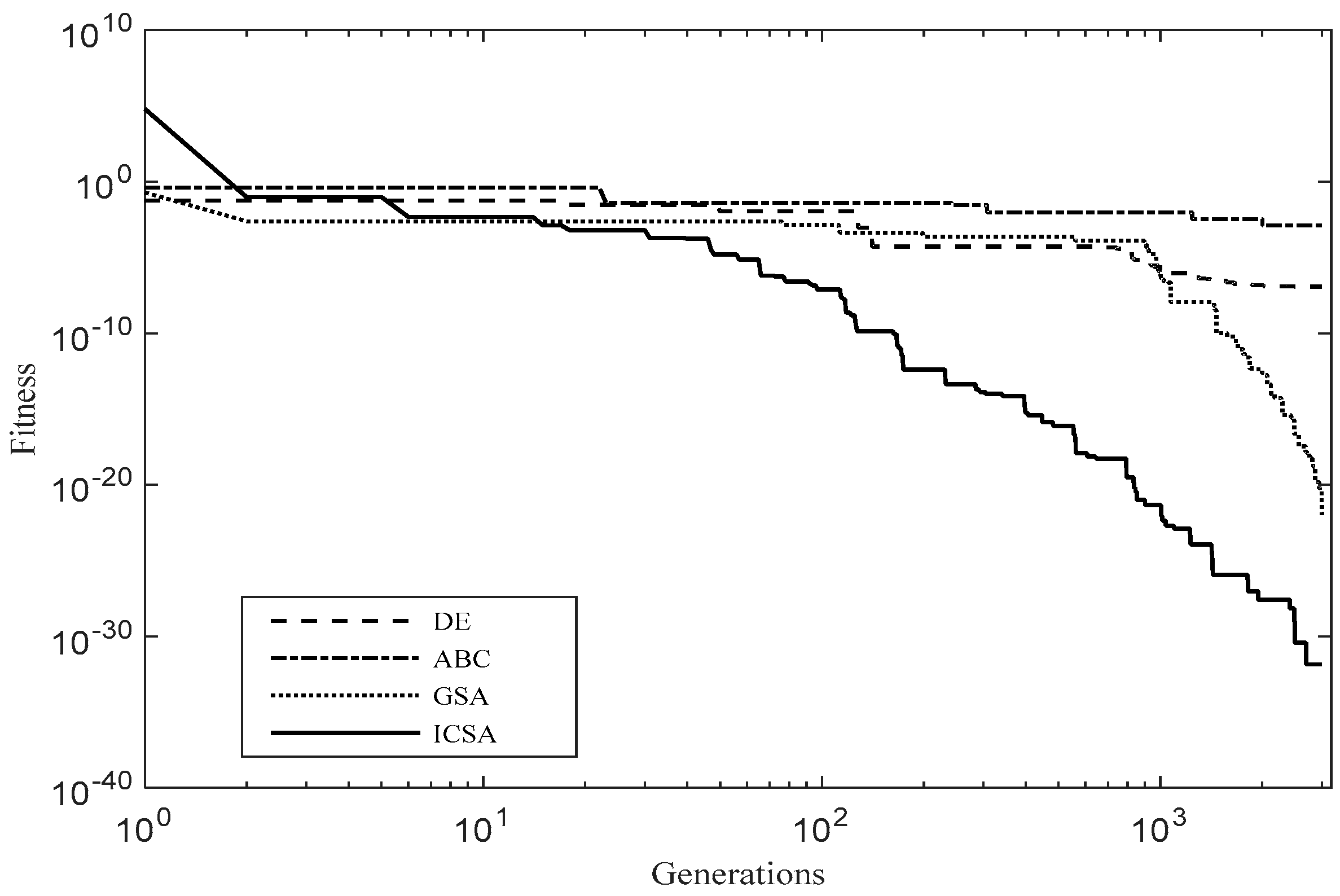
Figure 7.
10-bus distribution test system.
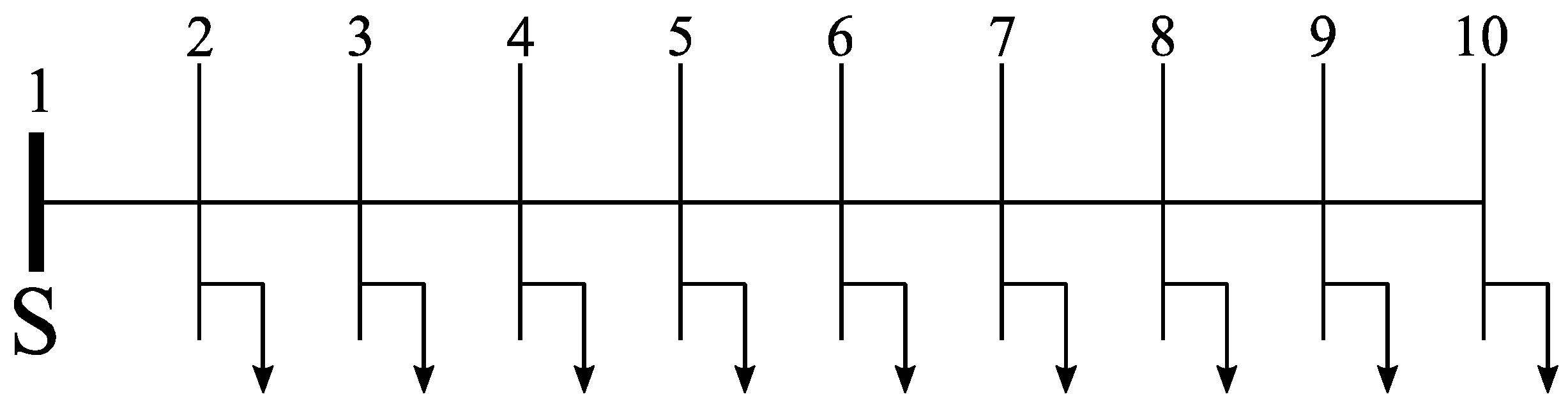
Figure 8.
Convergence comparison 10-bus.

Figure 9.
33-Bus distribution test system.

Figure 10.
Convergence comparison 33-bus.

Figure 11.
69-Bus distribution test system.

Table 1.
Manufacturer’s motor data.
| Characteristics | Motor 1 | Motor 2 |
|---|---|---|
| Power, HP | 5 | 40 |
| Voltage, V | 400 | 400 |
| Current, A | 8 | 45 |
| Frequency, Hz | 50 | 50 |
| No. Poles | 4 | 4 |
| Full load split | 0.07 | 0.09 |
| Starting torque (Tstr) | 15 | 260 |
| Max. Torque (Tmax) | 42 | 370 |
| Stator current | 22 | 180 |
| Full load torque (Tfl) | 25 | 190 |
Table 2.
Algorithms Parameters.
| DE | ABC | GSA | ICSA |
|---|---|---|---|
| CR = 0.5 F = 0.2 | φni = 0.5 SN = 120 | Go = 100 Alpha = 20 | FL = 2.0 |
Table 3.
Sensitivity Analysis of FL parameter.
| Parameter | Analysis | Motor 2 Exact Model | Motor 2 Approximate Model | 10-Bus | 33-Bus | 69-Bus |
|---|---|---|---|---|---|---|
| FL = 1.0 | Min | 7.1142 × 10⁻³ | 1.4884 × 10⁻¹³ | 696.61 | 139.92 | 145.87 |
| Max | 1.1447 × 10⁻² | 2.6554 × 10⁻⁵ | 699.56 | 146.06 | 164.12 | |
| Mean | 7.2753 × 10⁻³ | 1.6165 × 10⁻⁵ | 697.22 | 140.52 | 147.89 | |
| Std. | 7.4248 × 10⁻⁴ | 5.6961 × 10⁻⁵ | 0.6749 | 1.4291 | 3.2862 | |
| FL = 1.5 | Min | 7.1142 × 10⁻³ | 0.0000 | 696.61 | 139.42 | 146.08 |
| Max | 7.2485× 10⁻³ | 2.6172 × 10⁻³ | 701.03 | 144.55 | 161.03 | |
| Mean | 7.1237 × 10⁻³ | 7.47886× 10⁻⁵ | 697.65 | 140.70 | 147.54 | |
| Std. | 2.5728 × 10⁻⁵ | 4.4239 × 10⁻⁴ | 0.8045 | 1.9417 | 2.8354 | |
| FL = 2.0 | Min | 7.1142 × 10⁻³ | 0.0000 | 696.61 | 139.21 | 145.77 |
| Max | 7.1142 × 10⁻³ | 1.1675 × 10⁻²⁵ | 698.07 | 140.31 | 156.36 | |
| Mean | 7.1142 × 10⁻³ | 3.4339 × 10⁻²⁷ | 696.76 | 139.49 | 146.20 | |
| Std. | 2.2919 × 10⁻¹¹ | 1.9726 × 10⁻²⁶ | 0.3808 | 1.9374 | 2.1202 | |
| FL = 2.5 | Min | 7.1142 × 10⁻³ | 4.3700 × 10⁻²⁷ | 696.82 | 140.40 | 145.91 |
| Max | 7.1170 × 10⁻³ | 2.3971 × 10⁻¹⁶ | 698.76 | 148.80 | 158.72 | |
| Mean | 7.1142 × 10⁻³ | 1.7077 × 10⁻¹⁷ | 697.89 | 141.21 | 147.49 | |
| Std. | 5.3411 × 10⁻⁷ | 5.0152 × 10⁻¹⁷ | 0.5282 | 2.069 | 2.5549 | |
| FL = 3.0 | Min | 7.1142 × 10⁻³ | 6.8124 × 10⁻²¹ | 696.78 | 140.45 | 145.96 |
| Max | 7.1121 × 10⁻³ | 2.9549 × 10⁻¹³ | 703.36 | 158.66 | 164.12 | |
| Mean | 7.1142 × 10⁻³ | 1.3936 × 10⁻¹⁴ | 697.25 | 141.40 | 147.32 | |
| Std. | 1.5398 × 10⁻⁷ | 5.1283 × 10⁻¹⁴ | 1.6921 | 3.309 | 3.2862 |
Table 4.
Results of approximate circuit model , for motor 1.
| Analysis | DE | ABC | GSA | ICSA |
|---|---|---|---|---|
| Mean | 1.5408 × 10⁻⁴ | 0.0030 | 5.4439 × 10⁻²¹ | 1.9404 × 10⁻³⁰ |
| Std. | 7.3369 × 10⁻⁴ | 0.0024 | 4.1473 × 10⁻²¹ | 1.0674 × 10⁻²⁹ |
| Min | 1.9687 × 10⁻¹⁵ | 2.5701 × 10⁻⁵ | 3.4768 × 10⁻²² | 1.4024 × 10⁻³² |
| Max | 0.0043 | 0.0126 | 1.6715 × 10⁻²⁰ | 6.3192 × 10⁻²⁹ |
Table 5.
Results of approximate circuit model , for motor 2.
| Analysis | DE | ABC | GSA | ICSA |
|---|---|---|---|---|
| Mean | 4.5700 × 10⁻⁴ | 0.0078 | 5.3373 × 10⁻¹⁹ | 3.4339 × 10⁻²⁷ |
| Std. | 0.0013 | 0.0055 | 3.8914 × 10⁻¹⁹ | 1.9726 × 10⁻²⁶ |
| Min | 1.1369 × 10⁻¹³ | 3.6127 × 10⁻⁴ | 3.7189 × 10⁻²⁰ | 0.0000 |
| Max | 0.0067 | 0.0251 | 1.4020 × 10⁻¹⁸ | 1.1675 × 10⁻²⁵ |
Table 6.
Results of exact circuit model CostEM for motor 1.
| Analysis | DE | ABC | GSA | ICSA |
|---|---|---|---|---|
| Mean | 0.0192 | 0.0231 | 0.0032 | 0.0019 |
| Std. | 0.0035 | 0.0103 | 0.0000 | 4.0313 × 10⁻¹⁶ |
| Min | 0.0172 | 0.0172 | 0.0032 | 0.0019 |
| Max | 0.0288 | 0.0477 | 0.0032 | 0.0019 |
Table 7.
Results of exact circuit model CostEM for motor 2.
| Analysis | DE | ABC | GSA | ICSA |
|---|---|---|---|---|
| Mean | 0.0190 | 0.0791 | 0.0094 | 0.0071 |
| Std. | 0.0057 | 0.0572 | 0.0043 | 2.2919 × 10⁻¹¹ |
| Min | 0.0091 | 0.0180 | 0.0071 | 0.0071 |
| Max | 0.0305 | 0.2720 | 0.0209 | 0.0071 |
Table 8.
Possible capacitor sizes and cost ($/kVAr).
| j | 1 | 2 | 3 | 4 | 5 | 6 | 7 | 8 | 9 |
|---|---|---|---|---|---|---|---|---|---|
| Q | 150 | 350 | 450 | 600 | 750 | 900 | 1050 | 1200 | 1350 |
| $/kVAr | 0.500 | 0.350 | 0.253 | 0.220 | 0.276 | 0.183 | 0.228 | 0.170 | 0.207 |
| j | 10 | 11 | 12 | 13 | 14 | 15 | 16 | 17 | 18 |
| Q | 1500 | 1650 | 1800 | 1950 | 2100 | 2250 | 2400 | 2550 | 2700 |
| $/kVAr | 0.201 | 0.193 | 0.187 | 0.211 | 0.176 | 0.197 | 0.170 | 0.189 | 0.187 |
| j | 19 | 20 | 21 | 22 | 23 | 24 | 25 | 26 | 27 |
| Q | 2850 | 3000 | 3150 | 3300 | 3450 | 3600 | 3750 | 3900 | 4050 |
| $/kVAr | 0.183 | 0.180 | 0.195 | 0.174 | 0.188 | 0.170 | 0.183 | 0.182 | 0.179 |
Table 9.
Experimental results of 10-bus system.
| Items Algorithms | Base Case | Compensated | |||
|---|---|---|---|---|---|
| DE | ABC | GSA | ICSA | ||
| Total Power Losses (PLOSS), kW | 783.77 | 700.24 | 697.18 | 699.67 | 696.76 |
| Total Power losses cost, $ | 131,673.36 | 117,640.32 | 117,126.24 | 117,544.56 | 117,055.68 |
| Optimal buses | - | 6, 5, 9, 10 | 6, 5, 10, 8 | 6, 5, 9, 10, 7 | 6, 5, 9, 10, 8 |
| Optimal capacitor size | - | 900, 4050, 600, 600 | 1200, 4050, 600, 600 | 1650, 3150, 600, 450, 150 | 1200, 3900, 150, 600, 450 |
| Total kVAr | - | 6150 | 6450 | 6000 | 6300 |
| Capacitor cost, $ | - | 1153.65 | 1192.95 | 1253.55 | 1189.8 |
| Total annual cost | 131,673.36 | 118,793.97 | 118,329.19 | 118,798.11 | 118,245.48 |
| Net saving, $ | - | 12,879.38 | 13,344.17 | 12,875.24 | 13,427.88 |
| % saving | 9.78 | 10.10 | 9.77 | 10.19 | |
| Minimum voltage, p.u. | 0.8375 (bus 10) | 0.9005 (bus 10) | 0.9001 (bus 10) | 0.9002 (bus 10) | 0.9000 (bus 10) |
| Maximum voltage, p.u. | 0.9929 (bus 2) | 0.9995 (bus 3) | 1.0001 (bus 3) | 0.9992 (bus 3) | 0.9997 (bus 3) |
Table 10.
Experiments results of ICSA over CSA in 10-bus system.
| Items Algorithms | Base Case | Experiment 1 | Experiment 2 | ||
|---|---|---|---|---|---|
| CSA | ICSA | CSA | ICSA | ||
| Total Power Losses (PLOSS), kW | 783.77 | 698.14 | 698.14 | 676.02 | 675.78 |
| Total Power losses cost, $ | 131,673.36 | 117,287.52 | 117,287.52 | 113,571.36 | 113,531.04 |
| Optimal buses | - | 5, 6, 10 | 5, 6, 10 | 3, 4, 5, 6, 7, 10 | 3, 4, 5, 6, 8, 10 |
| Optimal capacitor size | - | 4050, 1650, 750 | 4050, 1650, 750 | 4050, 2100, 1950, 900, 450, 600 | 4050, 2400, 1650, 1200, 450, 450 |
| Total kVAr | - | 6150 | 6450 | 10,050 | 10,200 |
| Capacitor cost, $ | - | 6450 | 6450 | 10,050 | 10,200 |
| Total annual cost | - | 118,537.92 | 118,537.92 | 115,487.91 | 115,414.14 |
| Net saving, $ | 131,673.36 | 13,135.43 | 13,135.43 | 16,185.44 | 16,259.21 |
| % saving | - | 9.9 | 9.9 | 12.29 | 12.35 |
| Minimum voltage, p.u. | 0.8375 (bus 10) | 0.9000 (bus 10) | 0.9000 (bus 10) | 0.9003 (bus 10) | 0.9000 (bus 10) |
| Maximum voltage, p.u. | 0.9929 (bus 2) | 1.0001 (bus 3) | 1.0001 (bus 3) | 1.0070 (bus 3) | 1.0070 (bus 3) |
Table 11.
Experimental results of 33-bus system.
| Items Algorithms | Base Case | Compensated | |||
|---|---|---|---|---|---|
| DE | ABC | GSA | ICSA | ||
| Total Power Losses (PLOSS), kW | 210.97 | 152.92 | 141.13 | 140.27 | 139.49 |
| Total Power losses cost, $ | 35,442.96 | 25,690.56 | 23,740.08 | 23,565.60 | 23,434.32 |
| Optimal buses | - | 6, 29, 30, 14 | 6, 29, 8, 13, 27, 31, 14 | 30, 26, 15 | 30, 7, 12, 15 |
| Optimal capacitor size | - | 350, 750, 350, 750 | 150, 150, 150, 150, 600, 450, 150 | 900, 450, 350 | 900, 600, 150, 150 |
| Total kVAr | - | 2200 | 1800 | 1700 | 1800 |
| Capacitor cost, $ | - | 659 | 620.85 | 401.05 | 446.70 |
| Total annual cost | 35,442.96 | 26,349.56 | 25,540.00 | 23,966.65 | 23,881.02 |
| Net saving, $ | - | 9093.39 | 9902.95 | 11,476.31 | 11,561.94 |
| % saving | - | 25.65 | 27.94 | 32.37 | 32.62 |
| Minimum voltage, p.u. | 0.9037 (bus 18) | 0.9518 (bus 18) | 0.9339 (bus 18) | 0.9348 (bus 18) | 0.9339 (bus 18) |
| Maximum voltage, p.u. | 0.9970 (bus 2) | 0.9977 (bus 2) | 0.9976 (bus 2) | 0.9975 (bus 2) | 0.9976 (bus 2) |
Table 12.
Possible capacitor sizes and cost ($/kVAr).
| j | 1 | 2 | 3 | 4 | 5 | 6 |
|---|---|---|---|---|---|---|
| Q | 150 | 300 | 450 | 600 | 750 | 900 |
| $/kVAr | 0.500 | 0.350 | 0.253 | 0.220 | 0.276 | 0.183 |
Table 13.
Experiment result of ICSA over CSA in 33-bus system.
| Items Algorithms | Base Case | Compensated | |
|---|---|---|---|
| CSA | ICSA | ||
| Total Power Losses (PLOSS), kW | 210.97 | 139.30 | 138.14 |
| Total Power losses cost, $ | 35,442.96 | 23,402.40 | 23,207.52 |
| Optimal buses | - | 11, 24, 30, 33 | 11, 24, 30, 33 |
| Optimal capacitor size | - | 600, 450, 600, 300 | 450, 450, 900, 150 |
| Total kVAr | - | 1950 | 1950 |
| Capacitor cost, $ | - | 482.85 | 467.40 |
| Total annual cost | 35,442.96 | 23,885.25 | 23,674.92 |
| Net saving, $ | - | 11,557.71 | 11,768.04 |
| % saving | - | 32.60 | 33.20 |
| Minimum voltage, p.u. | 0.9037 (bus 18) | 0.9336 (bus 18) | 0.9302 (bus 18) |
| Maximum voltage, p.u. | 0.9970 (bus 2) | 0.9976 (bus 2) | 0.9976 (bus 2) |
Table 14.
Experiment result of 69-bus system.
| Items Algorithms | Base Case | Compensated | |||
|---|---|---|---|---|---|
| DE | ABC | GSA | ICSA | ||
| Total Power Losses (PLOSS), kW | 225 | 210.02 | 149.36 | 147.1017 | 146.20 |
| Total Power losses cost, $ | 37,800.00 | 35,283.36 | 25,092.48 | 24,712.80 | 24,561.60 |
| Optimal buses | - | 57, 58, 64, 21, 63, 20, 62, 26 | 58, 59, 62, 24 | 61, 27, 22 | 57, 61, 18 |
| Optimal capacitor size | - | 750, 600, 900, 350, 150, 150, 350, 150 | 150, 150, 900, 150 | 1200, 150, 150 | 150, 1200, 350 |
| Total kVAr | - | 3400 | 1350 | 1500 | 1700 |
| Capacitor cost, $ | - | 973.70 | 389.70 | 354.00 | 401.50 |
| Total annual cost | 37,800.00 | 36,257.06 | 25,482.18 | 25,066.8 | 24,961.10 |
| Net saving, $ | - | 1542.94 | 12,317.82 | 12,733.20 | 12,836.90 |
| % saving | - | 4.08 | 32.58 | 33.69 | 33.96 |
| Minimum voltage, p.u. | 0.9091 (bus 65) | 0.9504 (bus 61) | 0.9287 (bus 65) | 0.9298 (bus 65) | 0.9313 (bus 65) |
| Maximum voltage, p.u. | 0.9999 (bus 2) | 0.9999 (bus 2) | 0.9999 (bus 2) | 0.9999 (bus 2) | 0.9999 (bus 2) |
Table 15.
Statistical Analysis.
| Wilcoxon | DE-ICSA | ABC-ICSA | GSA-ICSA |
|---|---|---|---|
| 10-Bus | 2.5576× 10⁻³⁴ | 2.4788× 10⁻³⁴ | 2.5566× 10⁻³⁴ |
| 33-Bus | 6.1019 × 10⁻³⁴ | 3.4570× 10⁻³² | 7.6490 × 10⁻²⁴ |
| 69-Bus | 1.0853 × 10⁻²⁹ | 8.6857× 10⁻²⁸ | 3.6802 × 10⁻²⁰ |
© 2018 by the authors. Licensee MDPI, Basel, Switzerland. This article is an open access article distributed under the terms and conditions of the Creative Commons Attribution (CC BY) license (http://creativecommons.org/licenses/by/4.0/).
Share and Cite
MDPI and ACS Style
Díaz, P.; Pérez-Cisneros, M.; Cuevas, E.; Avalos, O.; Gálvez, J.; Hinojosa, S.; Zaldivar, D. An Improved Crow Search Algorithm Applied to Energy Problems. Energies 2018, 11, 571. https://doi.org/10.3390/en11030571
AMA Style
Díaz P, Pérez-Cisneros M, Cuevas E, Avalos O, Gálvez J, Hinojosa S, Zaldivar D. An Improved Crow Search Algorithm Applied to Energy Problems. Energies. 2018; 11(3):571. https://doi.org/10.3390/en11030571
Chicago/Turabian StyleDíaz, Primitivo, Marco Pérez-Cisneros, Erik Cuevas, Omar Avalos, Jorge Gálvez, Salvador Hinojosa, and Daniel Zaldivar. 2018. "An Improved Crow Search Algorithm Applied to Energy Problems" Energies 11, no. 3: 571. https://doi.org/10.3390/en11030571
Note that from the first issue of 2016, this journal uses article numbers instead of page numbers. See further details here.