Study of Ground Heat Exchangers in the Form of Parallel Horizontal Pipes Embedded in the Ground


Faculty of Chemical Engineering and Technology, Cracow University of Technology, 31-155 Kraków, Poland
*
Author to whom correspondence should be addressed.
Energies 2018, 11(3), 491; https://doi.org/10.3390/en11030491
Submission received: 4 January 2018
/
Revised: 7 February 2018
/
Accepted: 22 February 2018
/
Published: 26 February 2018
(This article belongs to the Section L: Energy Sources)
Abstract
:In order to predict long-term changes in the temperature of the ground in which a horizontal ground heat exchanger has been installed, it is beneficial to implement simplified mathematical models of heat transfer. The possibility of using a one-dimensional equation of heat conduction while modelling heat transfer in a ground heat exchanger with horizontal pipes has been demonstrated in the work. A theoretical analysis based on the linear heat source model as well as experimental research works have been carried out. It has been concluded that the temperature profiles of the ground in which parallel pipes of the heat exchanger are placed do not significantly differ from the profiles for the heat exchanger in the form of a plate; in particular, this refers to large distances from the level in which the pipes are positioned, small distances between pipes axes and the long duration of the process. Discrepancies between the calculated temperature increases for pipe and plate exchangers varied significantly in the individual time intervals, and were approx. 20–30%. The conducted experiments have demonstrated that the temperature field around parallel pipes of the heat exchanger may be described by the linear heat source model. The compatibility of temperature maps that were determined theoretically and experimentally was satisfactory with a good degree of accuracy.
1. Introduction
Ground heat exchangers most frequently constitute a part of the installation with a heat pump, which extracts energy from the ground or injects it into the ground. The pipes of ground heat exchangers are most often positioned vertically or horizontally. The advantages of horizontal heat exchangers, as compared to heat exchangers with vertical pipes, include lower investment cost and the possibility to make use of ambient energy in order to compensate for ground heat deficits (or to offload excess heat).
A large number of ground-source heat pumps have been used in buildings due to high energy and environmental performances. Paper [1] presents the results of many-year studies on the operational effectiveness of heat pumps utilising various lower heat sources under real conditions. The average value of the obtained seasonal operational effectiveness coefficient for ground heat pumps, in which exchangers that were positioned both vertically and horizontally were used, amounted to approx. 3.88.
The ground partially plays the role of a heat accumulator, and not only of its source/sink. If the amount of heat transferred annually to the ground is comparable with the amount extracted from the ground, e.g., for heating purposes, then the problems of the ground cooling or overheating do not occur. However, most frequently the amounts of heat extracted from the ground and transferred to the ground are not comparable. In a moderate climate zone, more heat is usually extracted from the ground than is transferred to the ground, and frequently the heat is only extracted from the ground. Heat transfer between the surroundings and the ground plays a principal role in the compensation for the heat deficit, particularly in horizontal heat exchangers that are placed at a shallow depth below the ground surface. This work is focused on horizontal ground heat exchangers.
Horizontal heat exchangers are the subject of numerous works, both experimental and theoretical. The results of laboratory research works on various types of ground heat exchangers: slinky, spiral coil, and U-type are illustrated in work by Yoon et al. [2]. The research works were carried out in a 5 × 1 × 1 m steel box filled with sand. The numerical models for the slinky-type heat exchanger are presented in works by Fujii et al. [3] and Xiong et al. [4].
Works by Wu et al. [5] and Gonzalez et al. [6] illustrate the results of experiments regarding heat extraction from the ground through a horizontal ground heat exchanger. The considerable impact of the ground heat exchanger on the temperature and humidity of the ground in the vicinity of the pipes of the heat exchanger has been confirmed.
Ground heat exchangers are often used as a sink, and not only as a source of heat. The results of the research works and calculations regarding a horizontal ground heat exchanger installed for the purposes of air conditioning in a living space have been presented in a study by Naili et al. [7].
A simulation of the work of a two-level ground heat exchanger has been shown in a paper by Dasare and Saha [8]. It has been concluded that the work of such a heat exchanger is similar to the simultaneous work of two one-level heat exchangers and that the optimal distance between the levels is 1.2 m.
In the works by Chong et al. [9] and Naylor et al. [10], it was confirmed that the length of the pipes necessary to obtain the appropriate temperature of the working fluid with the determined conditions of extracting and supplying the heat is dependent, above all, on the resistance of the heat conduction of the ground where the pipes are placed. The principles of optimal design regarding horizontal ground heat exchangers based on the conducted simulations, experimental research works, and an economic analysis are presented in a study by Go et al. [11].
A paper by Neuberger et al. [12,13,14] shows the results of the measurements of average temperatures of the ground with an installed horizontal heat exchanger at the beginning and at the end of successive heating seasons; the measurements demonstrated the thermal stability of the ground as a source of heat. A linear heat exchanger and a slinky-type heat exchanger were analyzed.
Gan [15] presented an analysis of heat extraction from various depths of the ground and in different periods of time. When heat is extracted from the ground in winter conditions, a deeper positioning of pipes is more beneficial. When heat is extracted in a warmer period (e.g., in the summer to heat swimming pool water), it is more beneficial to position pipes near the ground surface.
The results of calculations for horizontal ground heat exchangers using the CFD (Computational Fluid Dynamics) code Fluent are shown in the paper by Congedo et al. [16]. The calculations were carried out for various shapes: linear, helical, and slinky. It was found that a helical heat exchanger arrangement is the best type of pipe arrangement.
In the paper by D’Arpa et al. [17], the profitability of the use of heat pumps coupled with ground exchangers in greenhouse farming in relation to conventional heating (fossil fuels) was proved. The applied solution can fully satisfy the winter heating requirements in a cost-effective way.
Results of experiments concerning the periodic collection of heat from the ground are presented in the paper by Di Sipio and Bertermann [18]. Ground temperatures were monitored both during the heat collection period, and in the stagnation (temperature equalisation) period.
The amounts of heat extracted from or transferred to the ground are related to its temperature changes. In the case of a heat exchanger with horizontal pipes, one may take into consideration two different problems regarding the issue: short- and long-term. In the first case, during the extraction of heat from the ground, this is about not applying too high heat flux, which might cause significant local cooling of the ground near the pipes. The other problem refers to longer time ranges. The extraction of a large amount of heat (per unit area of ground heat exchanger) during the heating season may lead to excessive cooling of the ground throughout the area where the heat exchanger is installed (global). This is unfavourable especially in the case of long heating seasons, due to the fact that the time of the ground thermal recovery in the summer period is too short. In a warm climate zone, however, there exists an opposite problem regarding the high heat flux transferred to the ground in the summer period.
Lowering the average ground temperature within the area of the installed horizontal heat exchanger is a long-term process. As time passes, however, its gets slower and slower since the cooled ground surface extracts more and more heat from the ambient air, thus partly compensating for the energy deficit [19].
There are possibilities to manage the heat that is present in the ground. One of such possibilities, which involves the combination of a ground heat exchanger with the storage of thermal energy in the ground, is presented by Bottarelli in the work [20]. In this case, the pipes of the ground heat exchanger were placed in trenches filled with encapsulated granular material undergoing phase changes. A mixture of two types of such materials was applied.
The temperature field near the ground heat exchanger is difficult to determine. It depends on: the heat flux extracted from and supplied to the ground, initial conditions in the ground, its physical properties, and the configuration of the exchanger pipes. In order to determine the temperature field, various analytical and numerical methods are applied. Simulation calculations of ground exchangers, presented in the literature, concern mainly short-term operation. The results of such calculations cannot be generalised onto any (multiannual) process duration, because after a one-year operation cycle, the ground temperature profile is not usually identical to the initial profile. Thus, it is required to carry out the simulation calculations for long (multiannual) durations of the heat transfer processes in the ground.
Computational methods usually yield approximate results due to the complexity of the process of heat transfer in such a configuration. It is beneficial to apply simplified mathematical models of heat transfer in order to model long-term changes in the ground temperature when a horizontal heat exchanger is installed. In horizontal ground heat exchangers, temperature gradients in the vertical direction are prevalent, which naturally suggests a possibility to simplify the transfer equations to one-dimensional equations, particularly while investigating long-term processes. In our paper, the possibility to use one-dimensional models of heat transfer was considered.
The purpose of this work is to analyze the possibilities of applying a one-dimensional heat conduction equation while modelling heat transfer in the ground in which a heat exchanger with horizontal pipes is installed. The application of such a model significantly facilitates calculations of long-term changes in ground temperatures. The possibility to use a one-dimensional model was proved by a comparison of calculated temperature profiles in the ground for a pipe exchanger and for an exchanger in the form of a flat plate. The work covers a theoretical analysis based on the linear source model, as well as experimental research works aiming to demonstrate that a simplified model of heat transfer may be applied to determine long-term changes in the ground temperature.
2. Mathematical Model
The considerations refer to the ground heat exchanger with horizontal pipes positioned at one level. In the case of long durations, local heterogeneities of the temperature field in horizontal directions become considerably smaller than the changes with the distance from the ground surface. In order to determine such changes, it is necessary to know the thermal properties of the ground, the heat flux extracted from or supplied to the ground, the boundary conditions on the ground surface, and the depth of pipe installation; however, the way that they are arranged is less important.
Equations of the ground exchanger model describe the heat transfer between the surface of the horizontal pipes of the heat exchanger and the ground in which the pipes are embedded. The temperature field resulting from such a configuration is three-dimensional. Assuming that the temperature changes along the axis of the pipes (z) are small, the problem becomes two-dimensional. The changes in the temperature of the working fluid may be accounted for by treating the pipes as a configuration of a number of objects that are connected in series with ideal mixing [19,21].
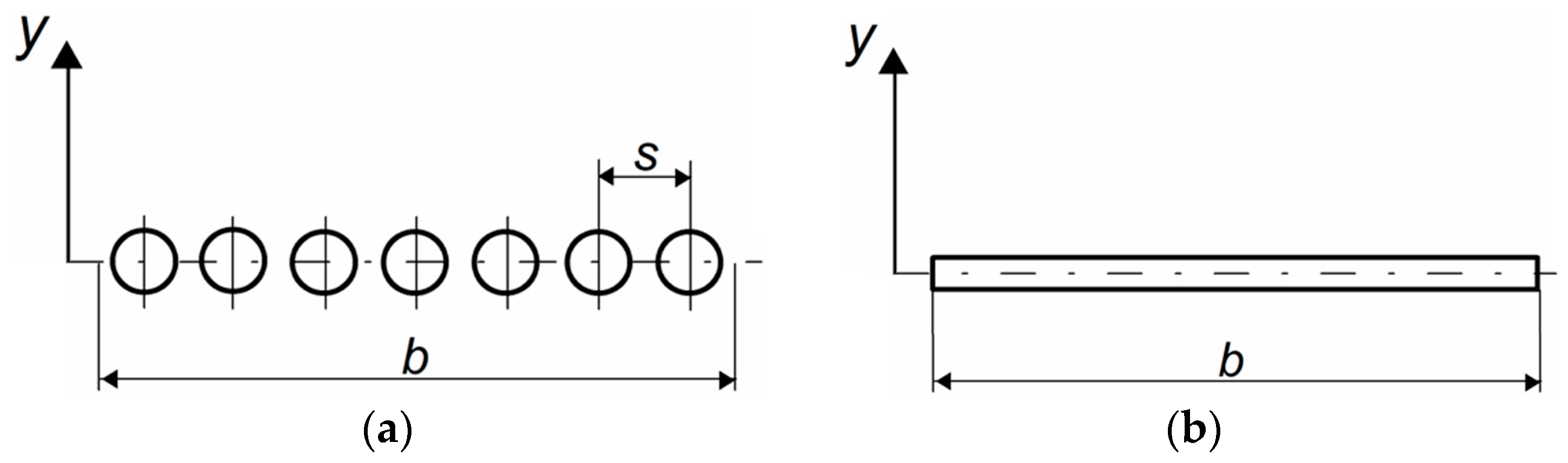
The problem may further be simplified by eliminating the position variable x (Figure 1a). If the pipes are arranged close to each other, then such a geometry, as far as heat transfer is concerned, demonstrates a similarity to a flat plate heated or cooled on both sides (Figure 1b).
In particular this refers to the layers of the ground that are placed away from the surface of the pipes and long process durations. Therefore, a ground heat exchanger in the form of m parallel pipes was taken into consideration. The width of the exchanger is b, and the distance between the axes of the pipes is s = b/m (Figure 2 and Figure 3). The initial ground temperature is homogeneous and is equal to Tinit. The feeding of the pipes with the working fluid is parallel, and the temperature changes of the working fluid along the length of the pipes are negligibly small. The absence of interaction between the ground surface and the surroundings was assumed. The heat flux transferred between the working fluid and the ground, referred to the length of the pipe, is equal to ql. A dependence, known as the linear source model [22,23], is valid for a single pipe:
where T is the ground temperature after a time t at a point distant by r from the pipe axis. The exponential integral is described:
and the method of its calculation is shown in Appendix A. For long process durations, the Ei function may be approximated with the following dependence (for ξ < 0.2):
where γ = 0.5772… is the Euler constant.
In Figure 2, a cross-section of system of m parallel pipes having the same spacing is shown. When the P point is at a large distance from the pipe installation level, the differences between the r1, r2, r3 ... lengths become insignificant.
The temperature at point P with coordinates (x, y) is equal:
The geometry of the configuration of parallel pipes positioned at equal s (Figure 2) leads to the conclusion that:
Therefore, the ground temperature depends on both the y and the x coordinates. In successive equations dimensionless quantities were introduced:
The dimensionless ground temperature increment amounts to:
where:
Alternatively, an exchanger in the form of a flat plate embedded in the ground was taken into consideration. Both exchangers (Figure 3) are of the same width and length.
If heat flux on the surface of the plate qs is constant, the ground temperature amounts to [22]:
where erfc is the complementary error function:
The dependence (13) refers to heat conduction in the semi-infinite body heated (or cooled) through a flat surface.
The amount of heat transferred in the pipe exchanger amounts to ql∙l∙m, where l stands for the length of the pipes. This amount of heat that is transferred in the plate exchanger corresponds with the heat flux qs. As the surface of the plate heat exchanger of the length l and the width b is equal to 2bl, the relation between ql and qs is as follows:
Using the dimensionless quantities, the following form of dependence (13) was obtained:
where:
3. Calculated Temperature Profiles
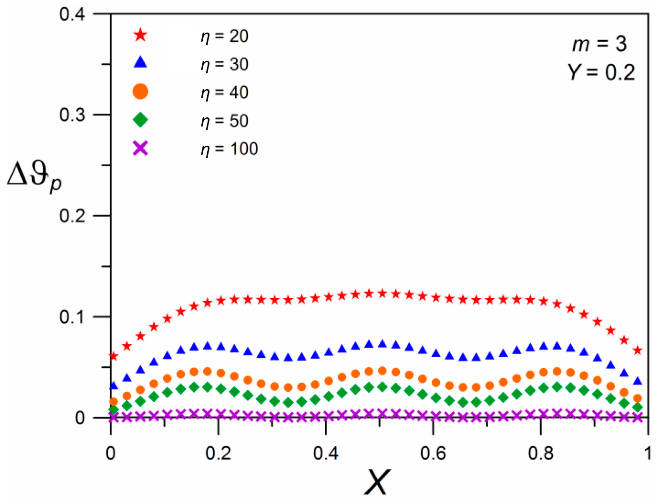
Figure 4, Figure 5 and Figure 6 illustrate the courses of dimensionless ground temperature increment dependencies Δθp, on the dimensionless position coordinate X for various values of the parameters η and Y as well as m. The η parameter is inversely proportional to time, the Y parameter is a dimensionless position coordinate in the vertical direction, whereas the m determines the distances between the pipes’ axes (given the specified width of the exchanger). In all of the cases, the temperatures are highly changeable with X near the extreme pipes, which results from diverse geometric conditions for these pipes in comparison with the pipes that are positioned in the central part of the exchanger.
Figure 4 illustrates the changes Δθp depending on X for various values η where the value of the position variable in the vertical direction is constant (Y = 0.2). It may be concluded that the longer the duration of the process (lower η), the smaller the temperature changes with the coordinate position X. Therefore, in the case of long process durations, the temperatures in the central part of the exchanger are almost even, similarly as in the case of the flat surface of the exchanger.
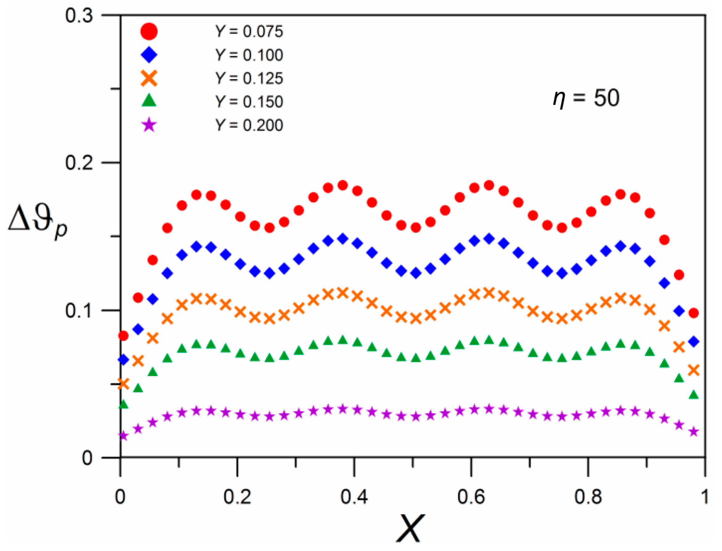
The values Δθp become smaller with the increase in Y, that is with the growing distance from the level where the pipes are embedded. This may be clearly observed in Figure 5. Moreover, with the increase of Y, the values Δθp (therefore, the ground temperature) become less and less dependent on X (with the exception of the regions near the values X = 0 and X = 1), so with the increase of Y the temperature profiles become more and more flat.
Figure 6 illustrates the courses of the dependence of Δθp on X for various numbers of pipes per specific width of the exchanger (so for various values of distances between the pipes’ axes). The larger m (smaller distances), the more even the temperatures alongside axis X. It is easy to recognize the number of pipes on the basis of the shape of the plot for m = 3 and m = 4. For the higher values of m, however, this becomes impossible. Large temperature increments for a larger number of pipes result from the larger amount of heat transferred in the exchanger.
The comparison of the temperature profiles in pipe and plate exchangers is presented in Figure 7. In order to determine the value of the temperature increment ΔT = T − Tinit, the following numerical values of the parameters were assumed: k = 1.3 W/(mK), α = 0.7 × 10⁻⁶ m2/s, b = 1 m, ql = 10 W/m, m = 5, y = 0.1 m. Values of temperatures increment ΔT for the heat exchanger in the form of a flat plate were calculated from the dependence (13). Inherently, these courses are independent of X.
For large values of y, i.e., large distances from the level of the pipe installation (Figure 2), approximately there is a relation rj = y; j = 1, 2, …, m. By substituting into the Equation (11) Rj ≈ Y the following was obtained:
Using the dependence (15) Δθp was converted into Δθs:
For long process durations, an approximate dependence (3) may be used; in this case, the linear source model equation has the following dimensionless form:
Figure 8 illustrates the courses of the dependence of Δθs on η for various values Y, determined on the basis of formulae for the pipe exchanger (19) and the plate exchanger (16).
As for the range within which the calculations were conducted, the compatibility is good, which confirms the fact that the temperature profiles in the ground with an installed pipe exchanger are similar to the profiles for an exchanger in the form of a flat plate.
Example results of calculations concerning discrepancies between the ground temperatures with pipe and plate exchangers embedded are presented. The calculations were carried out for the following parameter values: k = 1.3 W/(mK), α = 0.7 × 10⁻⁶ m2/s, ql = 10 W/m, b = 1 m, m = 5 for a process duration of t = 12 days and a distance from the exchanger’s surface of y = 0.6 m. For these conditions, η = 3.4 and Y = 0.6 were determined according to Equations (7) and (9). In Figure 8, Δθs = 0.024 (according to Equation (19)) for a pipe exchanger, and Δθs = 0.019 (according to Equation (16)) for a plate exchanger correspond to these values. After converting them to dimensional values, the following ground temperature increments were obtained according to Equation (17): 0.47 K and 0.37 K for a pipe exchanger and for a plate exchanger, respectively. Thus, in the considered case, the discrepancy between the determined value of the temperature increment for a pipe exchanger and for a plate exchanger is in the order of 20%.
In Figure 9, a comparison of courses of non-dimensional temperature increments depending on Y and η for the range of low η values, corresponding to long process durations, is shown. Also, courses corresponding to Equation (20) are shown for comparison.
The discrepancies between the courses for pipe and plate exchangers are difficult to characterise quantitatively; they are different in the individual time ranges. For example, for η = 0.68 (i.e., the value corresponding to a time of t = 60 days for b = 1 m), Δθs = 0.28 (according to Equation (19)) was obtained for a pipe exchanger, while Δθs = 0.36 (according to Equation (16)) was obtained for a plate exchanger. These values are shown in Figure 9. After converting to dimensional values, according to (17), the following ground temperature increments were obtained: 5.4 K and 6.9 K, for a pipe exchanger and for a plate exchanger, respectively, corresponding to a relative error of approx. 28%.
4. Experimental System
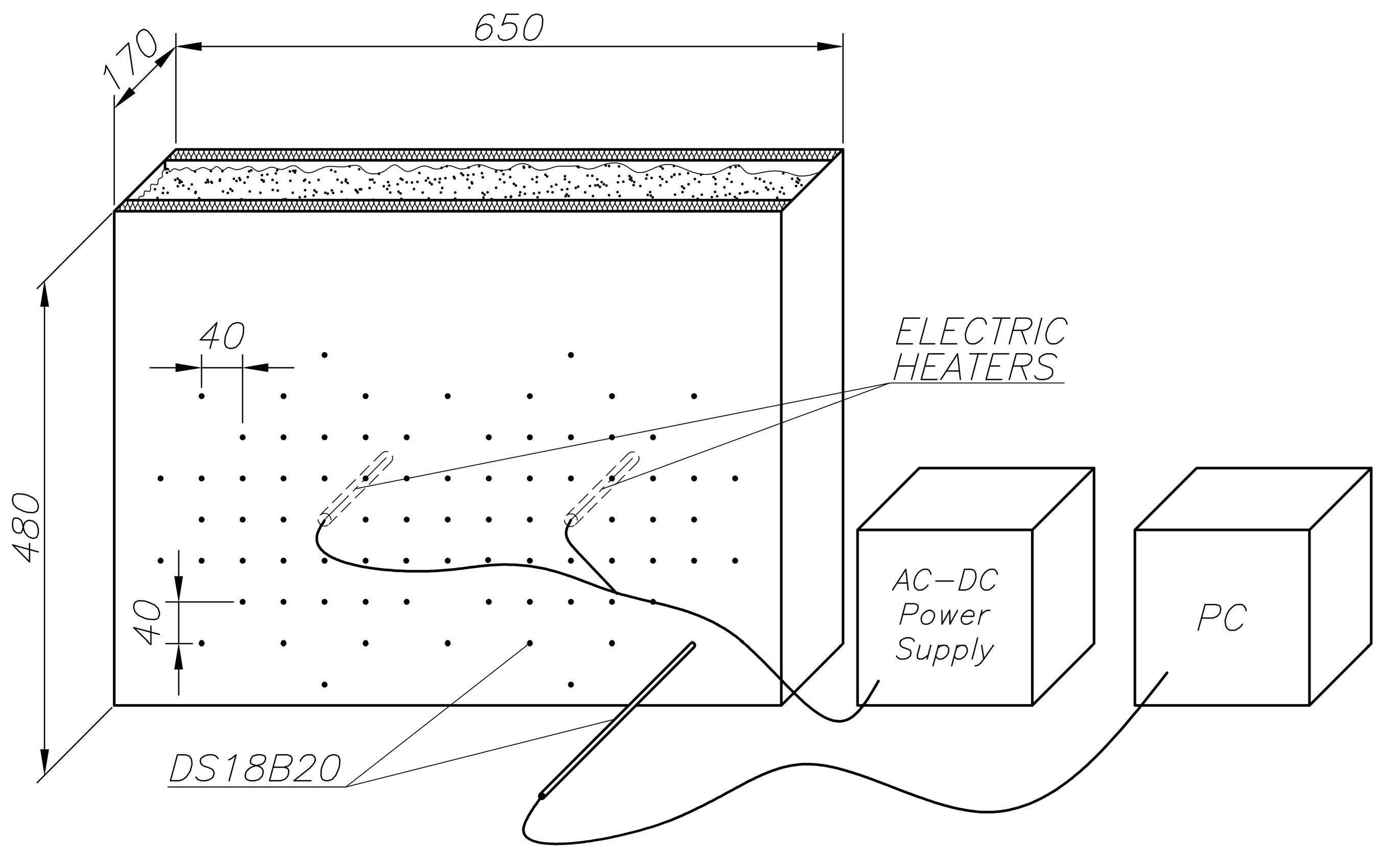
The computational courses of temperatures illustrated in the previous chapter are based on the linear heat source model. In order to experimentally verify the model, measurements of temperatures of granular material in the laboratory experimental installation presented in Figure 10 were carried out. The test system consisted of two electric heaters 12 mm in diameter and 110 mm in length, positioned in a container that was filled with granular material (quartz sand). The outer dimensions of the rectangular container made of acrylic glass plates 10 mm thick were 650 × 480 × 170 mm (width × height × thickness). The front walls of the container were insulated inside with expanded polystyrene 20 mm thick.
The heat output of each of the electric heaters was 5.3 W, and the distance between their axes was 240 mm. Seventy-nine digital temperature sensors DS18B20 with a tolerance ±0.5 °C within the temperature range from −10 °C to +85 °C were installed around the electric heaters. The distance between particular sensors was equal to 40 mm, and their distribution is shown in Figure 10. The signals from particular sensors were transferred through wires to the data acquisition system (Lämpömittari). The temperature measurements were made every 5 min from all of the sensors. A photograph of the research installation is presented in Figure 11.
5. Comparison of Experimental and Computational Results
On the basis of the obtained temperature measurement results in the granular bed depending on the position and time, the thermal parameters of the system were determined: thermal diffusivity α and the coefficient of thermal conductivity k. In the calculation procedure, the parameter values were adjusted so as to minimize the sum of the squared deviations of the values of experimental Texp and calculative Tcalc temperatures, i.e., the function:
where n is the number of measurement data.
The computational values of temperature were determined with the application of the linear source model. The Gauss-Seidel algorithm was used as the minimizing procedure, which consisted in alternating the search for the function minimum with respect to one, and next, the other variable. While searching for the minimum with respect to the variable k, the value α determined in the previous step and vice versa was assumed. The procedure was convergent and every time resulted in finding the thermal parameters of the system. The following assumptions were made for the calculations: ql = 48.2 W/m, s = 0.24 m, m = 2 and Tinit = 21.49 °C.
The results of the calculations for four sensors are presented in Table 1 which illustrates the following, in sequence: position coordinates for particular sensors, determined thermal parameters and the matching error specified on the basis of the minimizing value of the SS function.
Figure 12 illustrates a comparison of time courses of experimental temperatures with calculated temperatures for four sensors. As can be observed, the matching for long process durations is good, but in the case of short durations the computational values are slightly overestimated.
Also, the thermal parameters of the system combined for all of the sensors and for the specified process duration were determined. The application of the above-presented algorithm with the use of the temperature values obtained after 8 h of heating for all of the sensors yielded the following results: α = 0.399 × 10⁻⁶ m2/s, k = 0.522 W/(mK). These data were then used to generate temperature values for all of the sensors after 8 h of heating. The obtained map of temperatures on the x-y plane is illustrated in Figure 13. In comparison, Figure 14 shows the map of temperatures as determined experimentally. The compatibility of the isolines courses is satisfactory. Absolute error of the Tcalc determination did not exceed 3.5 K.
6. Conclusions
The main goal of the paper was to prove the possibility to use a one-dimensional heat transfer equation in a model of a horizontal ground exchanger. The possibility to use a one-dimensional model was proved when comparing the calculated temperature profiles in the ground for a pipe exchanger and an exchanger in the form of a flat plate.
To enable the use of a one-dimensional heat transfer equation, it was necessary to verify it underground exchanger conditions. A comparison with the linear source model was used. As the linear source model is also an approximate model, qualitative conformance of both models was the focus. The results shown in Figure 8 and Figure 9 confirm the qualitative conformance of the models for a pipe exchanger and a plate exchanger. Quantitative discrepancies of the courses between the models were evaluated approximately: they were different in the individual time ranges, and were approx. 20–30%. For long process durations, the temperature profile shapes for a pipe exchanger approximated rectilinear courses, corresponding to a plate exchanger.
In the case of small distances as compared to the depth of installation between horizontal pipes, the changeability of the ground temperature in the horizontal direction, perpendicular to the axes of the pipes, is not large. This is particularly clear in the case of long process durations.
The temperature profiles of the ground in which the parallel pipes of the heat exchanger are embedded do not significantly differ from the profiles for the exchanger in the form of a flat plate; in particular, this refers to large distances from the surface in which the pipes are embedded, small distances between the axes of the pipes, and long process durations.
The conducted experiments have demonstrated that the temperature field around parallel pipes of the heat exchanger may be described by the linear heat source model. The compatibility of temperature maps determined theoretically and experimentally was satisfactory, with a good degree of accuracy.
In order to analyze long-term changes in the temperature of the ground with an installed horizontal ground exchanger, it is possible to apply the model of heat transfer in the ground, which is based on a one-dimensional equation of heat conduction in the infinite plate.
Acknowledgments
The paper was supported by Cracow University of Technology, Poland by the provision of funds to cover the costs to publish in open access.
Author Contributions
Sebastian Pater analyzed the data and wrote the paper; Krzysztof Neupauer designed the experimental installation, performed the experiments and contributed to data collection; Krzysztof Kupiec conceived and designed the research.
Conflicts of Interest
The authors declare no conflict of interest.
Nomenclature
| b | width of heat exchanger, m |
| Ei | exponential integral |
| erfc | complementary error function |
| k | ground thermal conductivity, W/(mK) |
| l | length of heat exchanger, m |
| m | number of heat exchanger pipes |
| n | the number of measurement data |
| ql | heat stream per unit length of the pipe, W/m |
| qs | heat flux, W/m2 |
| P | point with coordinates (x, y) |
| heat stream, W | |
| r | distance between the point P and the pipe axis, m |
| R | dimensionless distance between the point P and the pipe axis (defined by Equation (8)) |
| s | distance between the axes of the exchanger pipes, m |
| SS | sum of squares |
| t | time, s |
| T | temperature of the ground, °C, |
| Tcalc | temperature calculated, °C, |
| Texp | temperature determined experimentally, °C, |
| Tinit | initial temperature of the ground, °C, |
| x | position coordinate (horizontal), m |
| X | dimensionless x-coordinate |
| y | position coordinate (vertical), m |
| Y | dimensionless y-coordinate |
| z | position coordinate, m |
| α | thermal diffusivity of the ground, m2/s |
| γ | the Euler constant |
| η | dimensionless parameter (defined by Equation (9)) |
| ΔT | temperature increment, K |
| Δθp | dimensionless temperature increment (defined by Equation(10)) |
| Δθs | dimensionless temperature increment (defined by Equation(17)) |
| σ | standard deviation |
Appendix A. Exponential Integral
The exponential integral is described in Equation (A1):
The improper integral given as follows (A2):
can be calculated numerically using the Gauss-Laguerre algorithm. Between the integrals in (A1) and (A2) there is a relationship:
Therefore,
whereas function f should be substituted (A5):
References
- Miara, M.; Günther, D.; Kramer, T.; Oltersdorf, T.; Wapler, J. Heat Pump Efficiency Analysis and Evaluation of Heat Pump Efficiency in Real-life Conditions. 2011, pp. 1–44. Available online: https://wp-monitoring.ise.fraunhofer.de/wp-effizienz/download/final_report_wp_effizienz_en.pdf (accessed on 1 February 2018).
- Yoon, S.; Lee, S.-R.; Go, G.-H. Evaluation of thermal efficiency in different types of horizontal ground heat exchangers. Energy Build. 2015, 105, 100–105. [Google Scholar] [CrossRef]
- Fujii, H.; Nishi, K.; Komaniwa, Y.; Chou, N. Numerical modeling of slinky-coil horizontal ground heat exchangers. Geothermics 2012, 41, 55–62. [Google Scholar] [CrossRef]
- Xiong, Z.; Fisher, D.E.; Spitler, J.D. Development and validation of a slinky ground heat exchanger model. Appl. Energy 2015, 141, 57–69. [Google Scholar] [CrossRef]
- Wu, Y.; Gan, G.; Verhoef, A.; Vidale, P.L.; Gonzalez, R.G. Experimental measurement and numerical simulation of horizontal-coupled slinky ground source heat exchangers. Appl. Therm. Eng. 2010, 30, 2574–2583. [Google Scholar] [CrossRef]
- Gonzalez, R.G.; Verhoef, A.; Vidale, P.L.; Main, B.; Gan, G.; Wu, Y. Interactions between the physical soil environment and a horizontal ground coupled heat pump for a domestic site in the UK. Renew. Energy 2012, 44, 141–153. [Google Scholar] [CrossRef]
- Naili, N.; Hazami, M.; Kooli, S.; Farhat, A. Energy and exergy analysis of horizontal ground heat exchanger for hot climatic condition of northern Tunisia. Geothermics 2015, 53, 270–280. [Google Scholar] [CrossRef]
- Dasare, R.R.; Saha, S.K. Numerical study of horizontal ground heat exchanger for high energy demand applications. Appl. Therm. Eng. 2015, 85, 252–263. [Google Scholar] [CrossRef]
- Chong, C.S.A.; Gan, G.; Verhoef, A.; Garcia, R.G.; Vidale, P.L. Simulation of thermal performance of horizontal slinky-loop heat exchangers for ground source heat pumps. Appl. Energy 2013, 104, 603–610. [Google Scholar] [CrossRef]
- Naylor, S.; Ellett, K.M.; Gustin, A.R. Spatiotemporal variability of ground thermal properties in glacial sediments and implications for horizontal ground heat exchanger design. Renew. Energy 2015, 81, 21–30. [Google Scholar] [CrossRef]
- Go, G.-H.; Lee, S.-R.; Yoon, S.; Kim, M.-J. Optimum design of horizontal ground-coupled heat pump systems using spiral-coil-loop heat exchangers. Appl. Energy 2016, 162, 330–345. [Google Scholar] [CrossRef]
- Neuberger, P.; Adamovský, R.; Šeďová, M. Temperatures and heat flows in a soil enclosing a slinky horizontal heat exchanger. Energies 2014, 7, 972–987. [Google Scholar] [CrossRef]
- Pauli, P.; Neuberger, P.; Adamovský, R. Monitoring and analysing changes in temperature and energy in the ground with installed horizontal ground heat exchangers. Energies 2016, 9, 555. [Google Scholar] [CrossRef]
- Neuberger, P.; Adamovsky, R. Analysis of the potential of low-temperature heat pump energy sources. Energies 2017, 10, 1922. [Google Scholar] [CrossRef]
- Gan, G. Dynamic thermal modelling of horizontal ground-source heat pumps. Int. J. Low Carbon Technol. 2013, 8, 95–105. [Google Scholar] [CrossRef]
- Congedo, P.M.; Colangelo, G.; Starace, G. CFD simulations of horizontal ground heat exchangers: A comparison among different configurations. Appl. Therm. Eng. 2012, 33, 24–32. [Google Scholar] [CrossRef]
- D’Arpa, S.; Colangelo, G.; Starace, G.; Petrosillo, I.; Bruno, D.E.; Uricchio, V.; Zurlini, G. Heating requirements in greenhouse farming in southern Italy: Evaluation of ground-source heat pump utilization compared to traditional heating. Energy Effic. 2015, 9, 1065–1085. [Google Scholar] [CrossRef]
- Di Sipio, E.; Bertermann, D. Factors influencing the thermal efficiency of horizontal ground heat exchangers. Energies 2017, 10, 1897. [Google Scholar] [CrossRef]
- Kupiec, K.; Larwa, B.; Gwadera, M. Heat transfer in horizontal ground heat exchangers. Appl. Therm. Eng. 2015, 75, 270–276. [Google Scholar] [CrossRef]
- Bottarelli, M.; Bortoloni, M.; Su, Y. Heat transfer analysis of underground thermal energy storage in shallow trenches filled with encapsulated phase change materials. Appl. Therm. Eng. 2015, 90, 1044–1051. [Google Scholar] [CrossRef]
- Kupiec, K.; Larwa, B.; Gwadera, M.; Komorowicz, T. Modelling of heat transfer in the ground. Przem. Chem. 2016, 95, 1997–2002. [Google Scholar] [CrossRef]
- Carslaw, H.S.; Jaeger, J.C. Conduction of Heat in Solids, 2nd ed.; Oxford University Press: London, UK, 1959; ISBN 978-0198533689. [Google Scholar]
- Conti, P. Dimensionless maps for the validity of analytical ground heat transfer models for GSHP applications. Energies 2016, 9, 890. [Google Scholar] [CrossRef]
Figure 1.
Considered systems: (a) Parallel pipes configuration; (b) Flat plate.
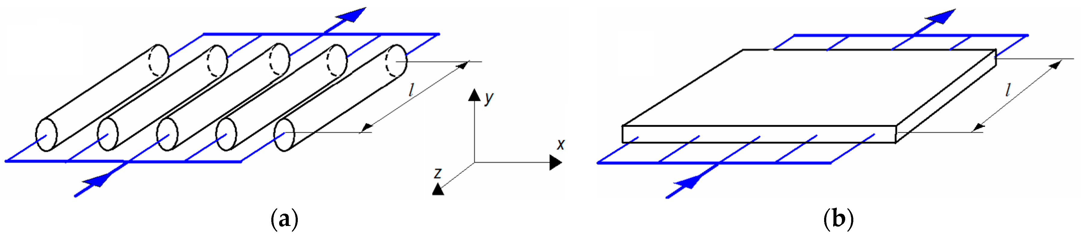
Figure 2.
The parallel pipes system of a ground heat exchanger.
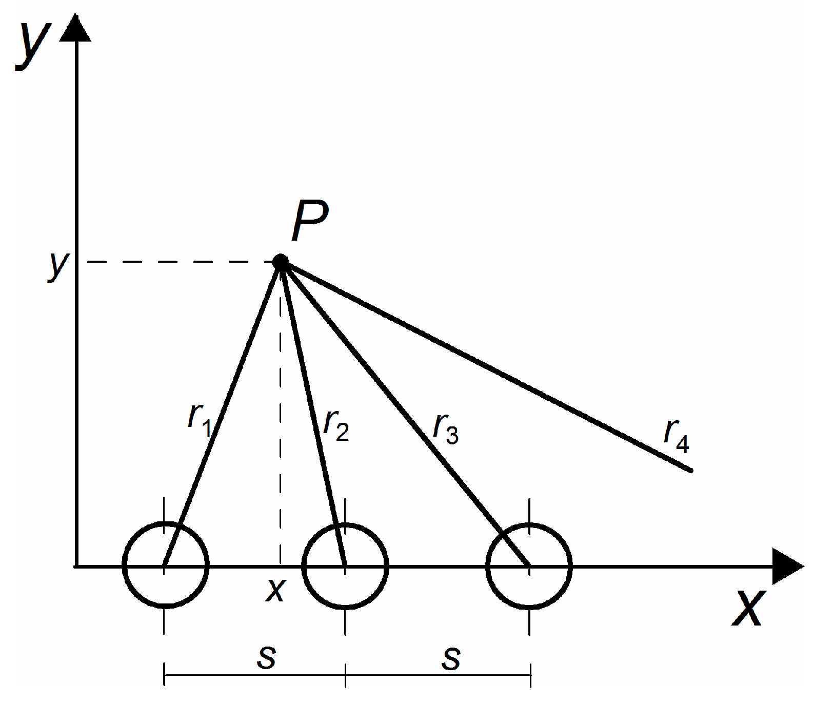
Figure 3.
(a) Parallel pipes configuration; (b) Flat plate.

Figure 4.
Dependence of dimensionless ground temperature increment Δθp on the dimensionless position coordinate X for various values of η.
Figure 4.
Dependence of dimensionless ground temperature increment Δθp on the dimensionless position coordinate X for various values of η.

Figure 5.
Dependence of dimensionless ground temperature increment Δθp on the dimensionless position coordinate X for various values of Y.
Figure 5.
Dependence of dimensionless ground temperature increment Δθp on the dimensionless position coordinate X for various values of Y.

Figure 6.
Dependence of dimensionless ground temperature increment Δθp on the dimensionless position coordinate X for various values of m.
Figure 6.
Dependence of dimensionless ground temperature increment Δθp on the dimensionless position coordinate X for various values of m.
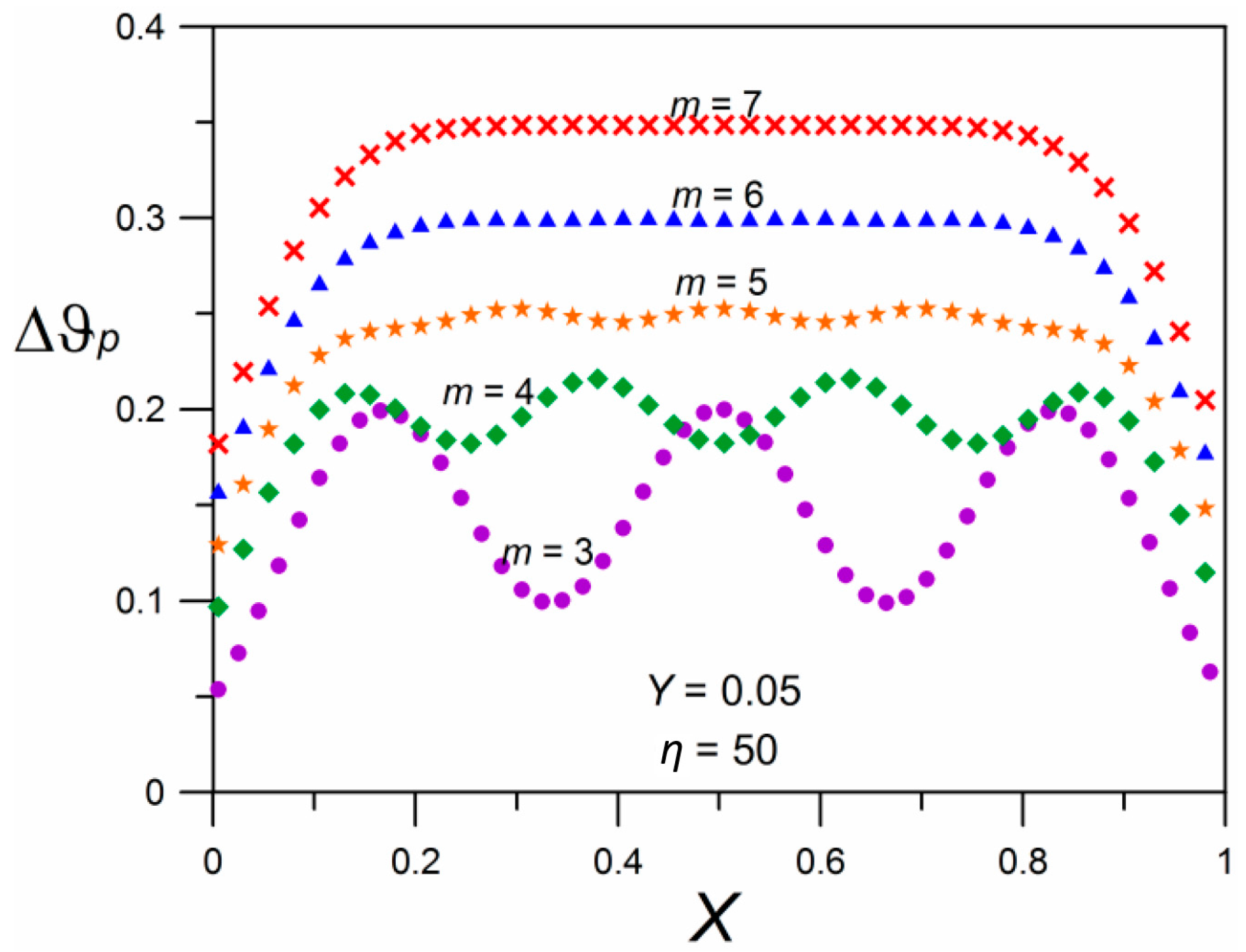
Figure 7.
The comparison of the ground temperature increment ΔT for pipe exchanger and flat plate exchanger.
Figure 7.
The comparison of the ground temperature increment ΔT for pipe exchanger and flat plate exchanger.
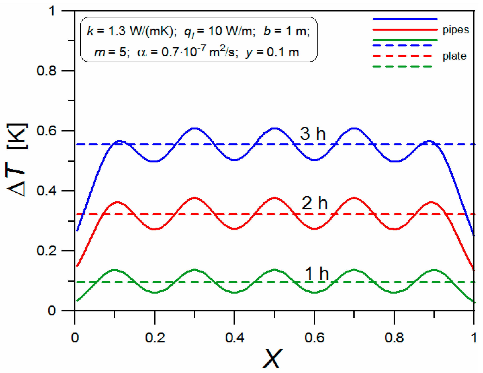
Figure 8.
Comparison of dependencies (16) and (19).
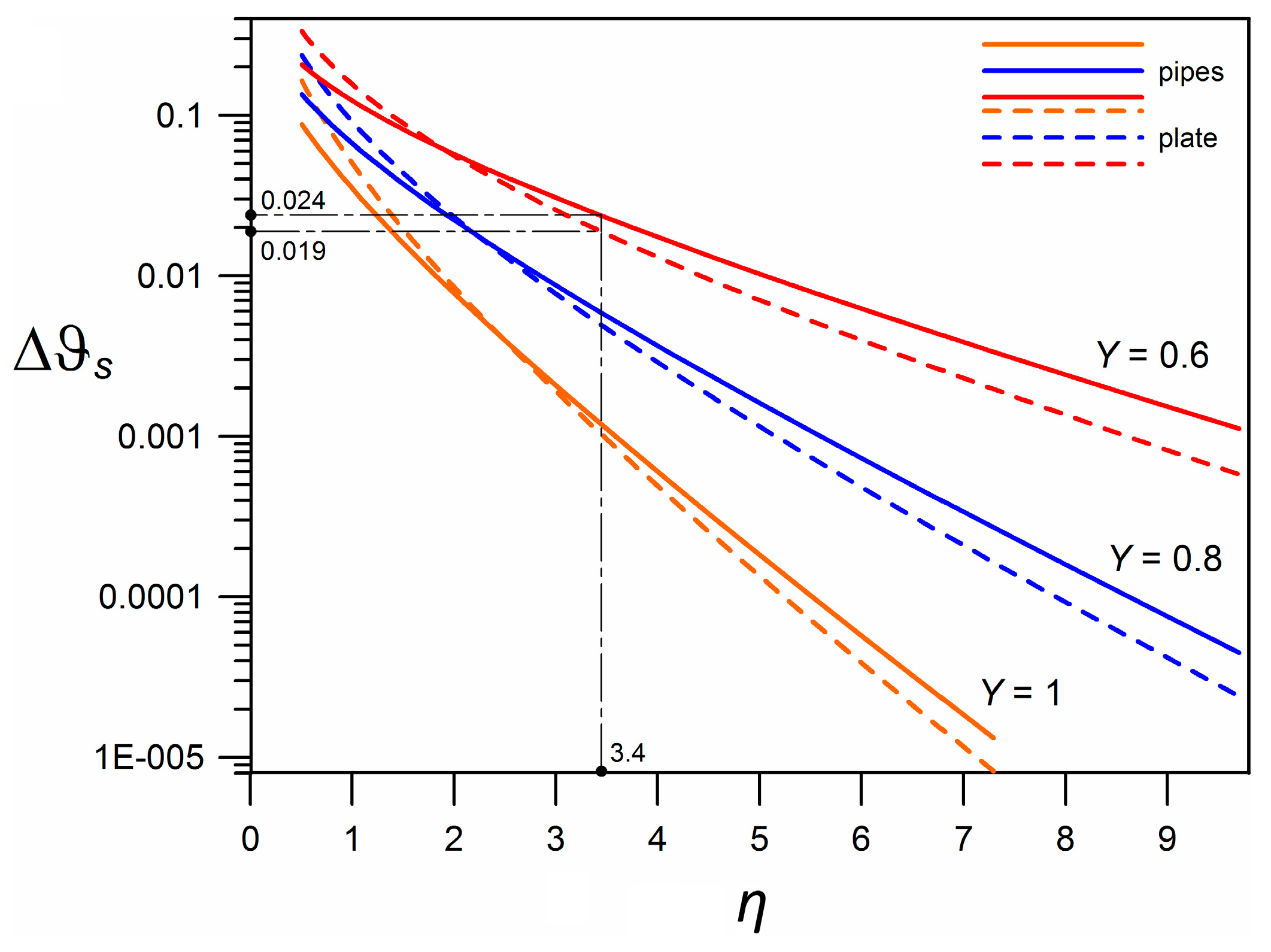
Figure 9.
Comparison of dependencies (16) and (19) for long process duration.
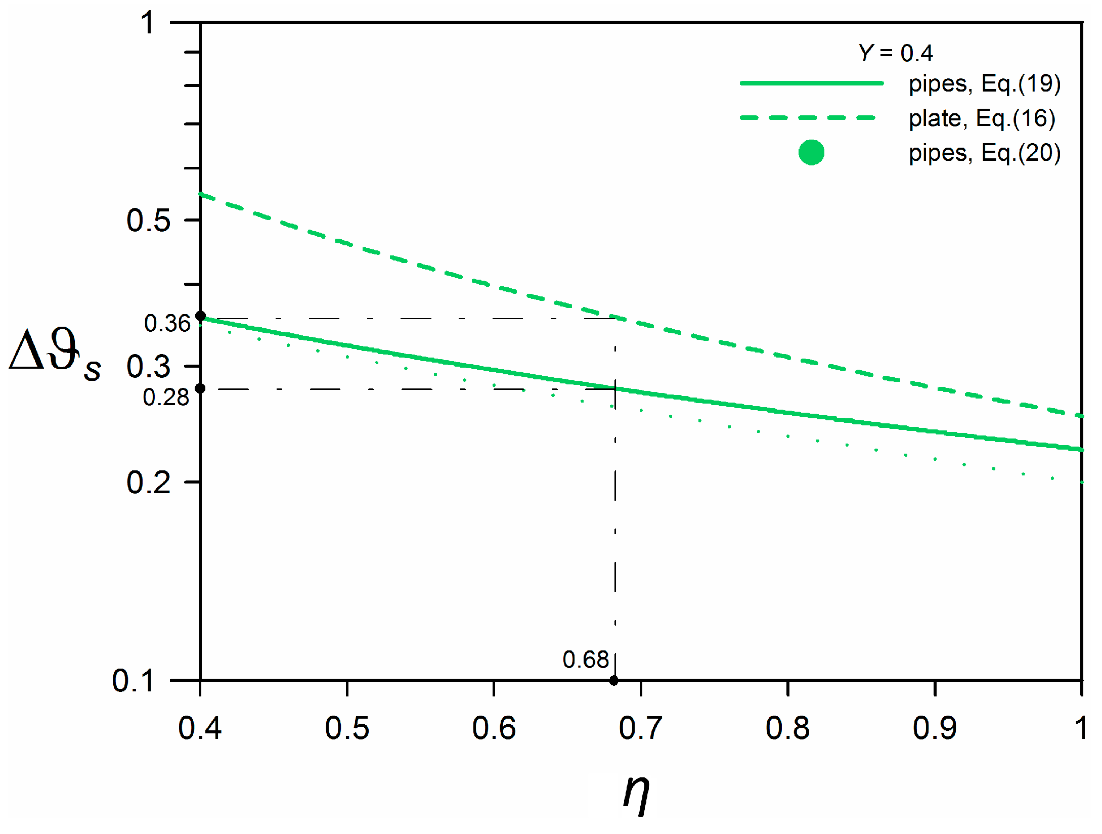
Figure 10.
Experiment system with location of temperature sensors.

Figure 11.
A photo of the research installation.
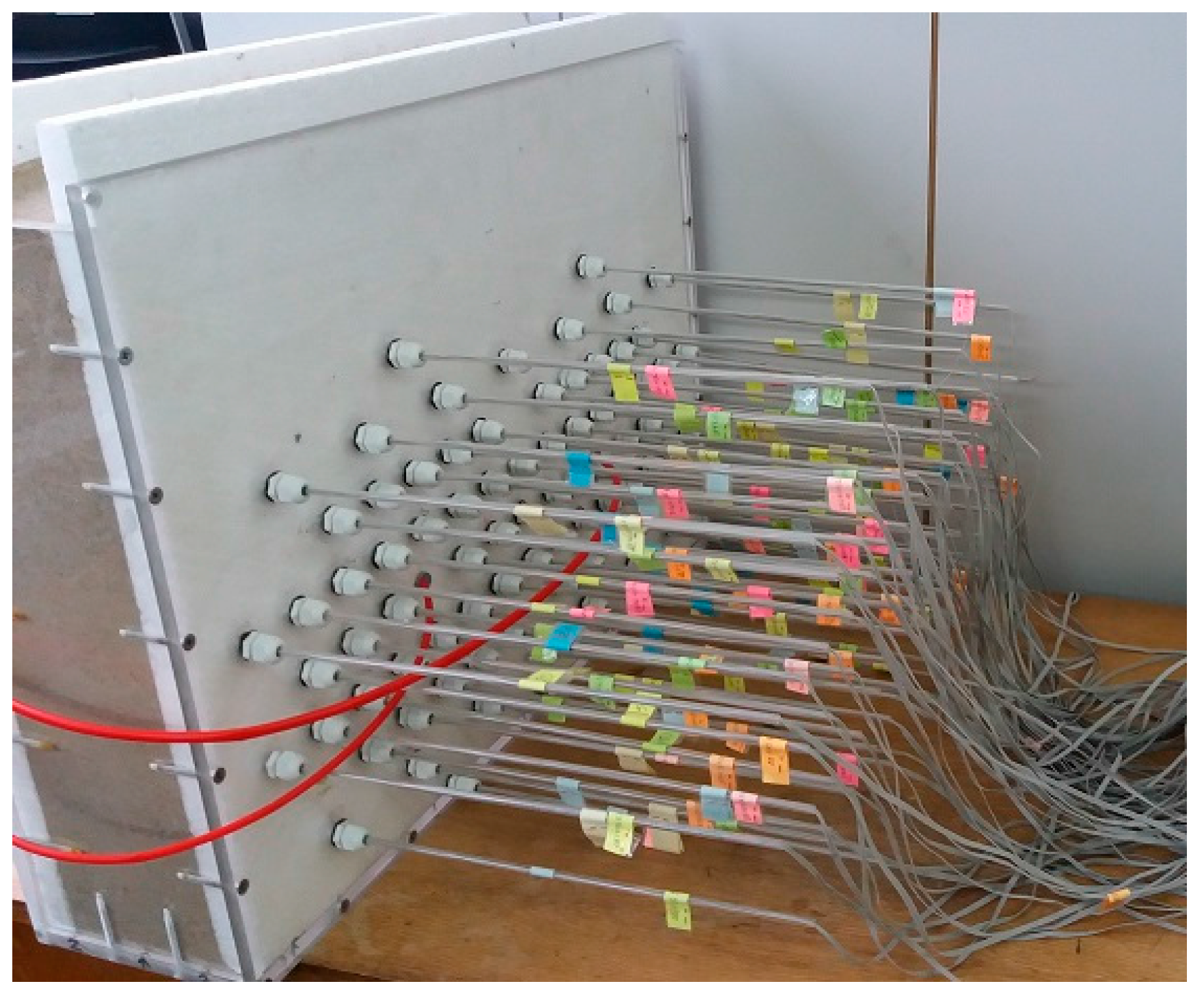
Figure 12.
Comparison of experimental and computational results.
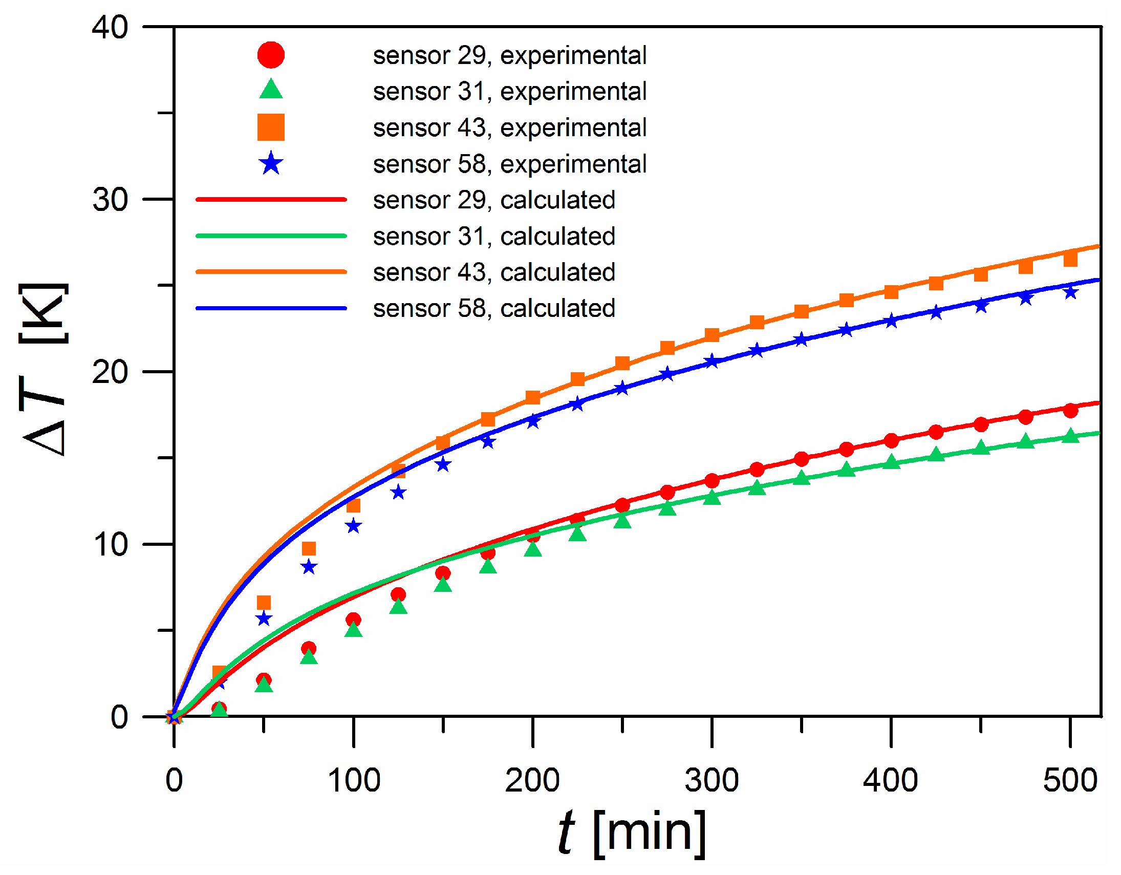
Figure 13.
Temperature maps on the x-y plane determined on the basis of theoretical calculations.

Figure 14.
Temperature maps on the x-y plane determined on the basis of experimental results.


Table 1.
Determined values of thermal parameters of the system.
| Sensor | x, m | y, m | α·106, m2/s | k, W/(mK) | σ, K |
|---|---|---|---|---|---|
| 29 | 0.32 | 0.04 | 0.589 | 0.650 | 0.06 |
| 31 | 0.40 | 0.04 | 0.723 | 0.714 | 0.14 |
| 43 | 0.32 | 0.00 | 0.757 | 0.584 | 0.25 |
| 58 | 0.36 | −0.04 | 0.686 | 0.572 | 0.19 |
© 2018 by the authors. Licensee MDPI, Basel, Switzerland. This article is an open access article distributed under the terms and conditions of the Creative Commons Attribution (CC BY) license (http://creativecommons.org/licenses/by/4.0/).
Share and Cite
MDPI and ACS Style
Neupauer, K.; Pater, S.; Kupiec, K. Study of Ground Heat Exchangers in the Form of Parallel Horizontal Pipes Embedded in the Ground. Energies 2018, 11, 491. https://doi.org/10.3390/en11030491
AMA Style
Neupauer K, Pater S, Kupiec K. Study of Ground Heat Exchangers in the Form of Parallel Horizontal Pipes Embedded in the Ground. Energies. 2018; 11(3):491. https://doi.org/10.3390/en11030491
Chicago/Turabian StyleNeupauer, Krzysztof, Sebastian Pater, and Krzysztof Kupiec. 2018. "Study of Ground Heat Exchangers in the Form of Parallel Horizontal Pipes Embedded in the Ground" Energies 11, no. 3: 491. https://doi.org/10.3390/en11030491
Note that from the first issue of 2016, this journal uses article numbers instead of page numbers. See further details here.