Development of a Data-Driven Predictive Model of Supply Air Temperature in an Air-Handling Unit for Conserving Energy

1
SH Urban Research Center, Seoul Housing & Communities Corporation, 621, Gaepo-ro, Gangnam-gu, Seoul 06336, Korea
2
Department of Architectural Engineering, Yonsei University, 50 Yonsei Street, Seodaemun-gu, Seoul 03722, Korea
*
Author to whom correspondence should be addressed.
Energies 2018, 11(2), 407; https://doi.org/10.3390/en11020407
Submission received: 29 December 2017
/
Revised: 24 January 2018
/
Accepted: 29 January 2018
/
Published: 9 February 2018
(This article belongs to the Special Issue Control and Nonlinear Dynamics on Energy Conversion Systems)
Abstract
:The purpose of this study was to develop a data-driven predictive model that can predict the supply air temperature (SAT) in an air-handling unit (AHU) by using a neural network. A case study was selected, and AHU operational data from December 2015 to November 2016 was collected. A data-driven predictive model was generated through an evolving process that consisted of an initial model, an optimal model, and an adaptive model. In order to develop the optimal model, input variables, the number of neurons and hidden layers, and the period of the training data set were considered. Since AHU data changes over time, an adaptive model, which has the ability to actively cope with constantly changing data, was developed. This adaptive model determined the model with the lowest mean square error (MSE) of the 91 models, which had two hidden layers and sets up a 12-hour test set at every prediction. The adaptive model used recently collected data as training data and utilized the sliding window technique rather than the accumulative data method. Furthermore, additional testing was performed to validate the adaptive model using AHU data from another building. The final adaptive model predicts SAT to a root mean square error (RMSE) of less than 0.6 °C.
1. Introduction
The prediction of energy use and indoor environmental quality, such as temperature and relative humidity in buildings, is important for achieving energy conservation and is also employed in heating, ventilating, and air-conditioning (HVAC) applications [1].
The energy consumption and indoor air temperature of buildings can be estimated using one of two models: (1) physical or white-box models; and (2) empirical or black-box models. Both models use weather parameters and actuators’ manipulated variables as inputs, with the predicted energy or temperature as their output [2,3]. The heating and cooling demand can be estimated by means of an energy simulation program, which can calculate the system capacity and zone temperature; this is what is referred to as physical modelling or white-box modelling. It is necessary to be aware of a building’s physical properties in order to create accurate models of the type mentioned above [4]. Physical models can be used to provide forecasts of indoor climate variables before an actual building is constructed. However, black-box modeling is a data mining technique used to extract information from models. Black-box models, such as neural networks, need experimental data, which can be obtained after the actual building is constructed and measurements are made available. Some combination models which use energy simulation and genetic algorithms can also be utilized to select optimal design parameters and conserve energy [5].
Several articles have been published on the incorporation of black-box artificial neural networks to predict room temperature and relative humidity. This data can then be used to design and operate HVAC control systems [6,7,8]. Mustafaraj et al. used autoregressive linear and nonlinear neural network models to predict the room temperature and relative humidity of an open office. External and internal climate data from over three months were used to validate the models, and results showed that both models provided reasonable predictions; however, the nonlinear neural network model was superior in predicting the two variables. These predictions can be used in control strategies to save energy where air-conditioning systems operate [4]. Indoor temperature data, predicted using neural networks by the application of the Levenberg-Marquardt algorithm, was used for the control of an air-conditioned system [2]. Additionally, Kim et al. were able to make quite accurate predictions for each zone's temperature using accumulated building operational data [9]. Zhao et al. reviewed many of the techniques used to predict building energy consumption. Of the many techniques used, the ones relevant to this study are: the engineering method, which uses computer simulations; neural networks, which use artificial intelligence concepts; Support Vector Machine (SVM), which produces relatively accurate results despite small quantities of training data; and grey models, which are used when there is incomplete or uncertain data [1].
Neto et al. compared building energy consumption predicted by using an artificial neural network (ANN) and a physical model for a simulation program. Their results are suitable for energy consumption prediction with error ranges for ANNs and simulation at 10% and 13%, respectively [10]. Kreider et al. concluded that, using a neural network, operation data alone can estimate electrical demand for assessing HVAC systems [11]. Miller et al. used ANNs to predict the optimum start time for a heating plant during a setback and compared the results of ANN prediction with the conventional recursive least-squares method [12,13]. Nakahar used three different load prediction models (Kalman filter, group method of data handling (GMDH), and neural network) to estimate load for the following day and hours, to install optimal thermal storage [14]. Using general regression neural networks, Ben-Nakhi successfully predicted the time of the end of a thermostat setback to restore the designated temperature inside a building, in time for the start of business hours [6]. According to Yang et al., when the ANN prediction model is used to research optimal start and stop operation methods for cooling systems, energy consumption can be successfully reduced by 3% and 18%, respectively. Based on past building operational data, learning concepts have been introduced with optimal start and stop points discovered through analysis [15]. Nabil developed self-tuning HVAC component models based on ANNs and validated against data collected from an existing HVAC system. Errors of these models are within 2–8% in terms of coefficient variance (CV). It has been shown that the optimization process can provide total energy savings of 11% [16]. Kuisak et al. developed a data-driven approach for a daily steam load model. They used a neural network and researched 10 different data-mining algorithms to develop a predictive model [17]. Predictive neural network models have also been developed for a chiller and ice thermal storage tank of a central plant HVAC system [18]. The machine learning algorithm of an ANN is often adapted to complicated and nonlinear systems such as HVAC systems [19]. The popularity of ANNs for various applications related to online control of HVAC systems and energy management in buildings, has been increasing in the past few years [2].
The purpose of the present study was to develop a model to predict supply air temperature (SAT) of an air-handling unit (AHU) by applying AHU-historical data to a neural network, one of the black box approaches.
This current study details the process of finding various methods for improving prediction performances. Therefore, the model developed in this study was considered an adaptive model using recent hourly-operational data. When the SAT of an AHU can be estimated, it is possible to calculate the accurate amount of energy either to be eliminated or to be supplied into a building. In addition, this model can be used to calculate the heating and cooling coil load. Results of this study can be applied to control strategies and operational management of AHUs in order to reduce energy consumption.
2. Development of Models
2.1. Neural Network
The present study used a typical neural network as shown in Figure 1. Since an ANN has the ability to learn and analyze mapping relations, including nonlinear ones, its application to resolve various difficult problems has been increasing rapidly [14].
There are three layers of neurons: an input, a hidden, and an output layer. In Figure 1, neurons are placed in multiple layers. The first layer (input layer) receives inputs from the outside. The third layer (output layer) supplies the result assessed by the network and organizes the responses obtained [10]. One or more layers, called hidden layers are positioned between the first layer and the third layer. The ANN has the ability to produce output which goes through a neuron’s network function. It can also match the produced output value to target value by modifying weights of interconnections. An ANN involves interconnected neurons. Each neuron or node is an independent computational unit. The current study used resilient backpropagation with weight backtracking for supervised learning in feedforward ANNs. Training a neural network is a process of setting the most suitable weights on the input of each unit. Backpropagation is the most used method for calculating error gradient for a feedforward network [20]. Connection weights and bias values initially selected as random numbers can be fixed as a result of the training process.
2.2. Data
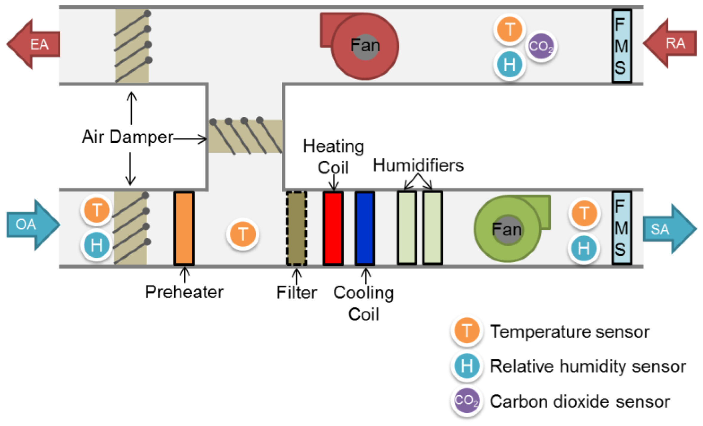
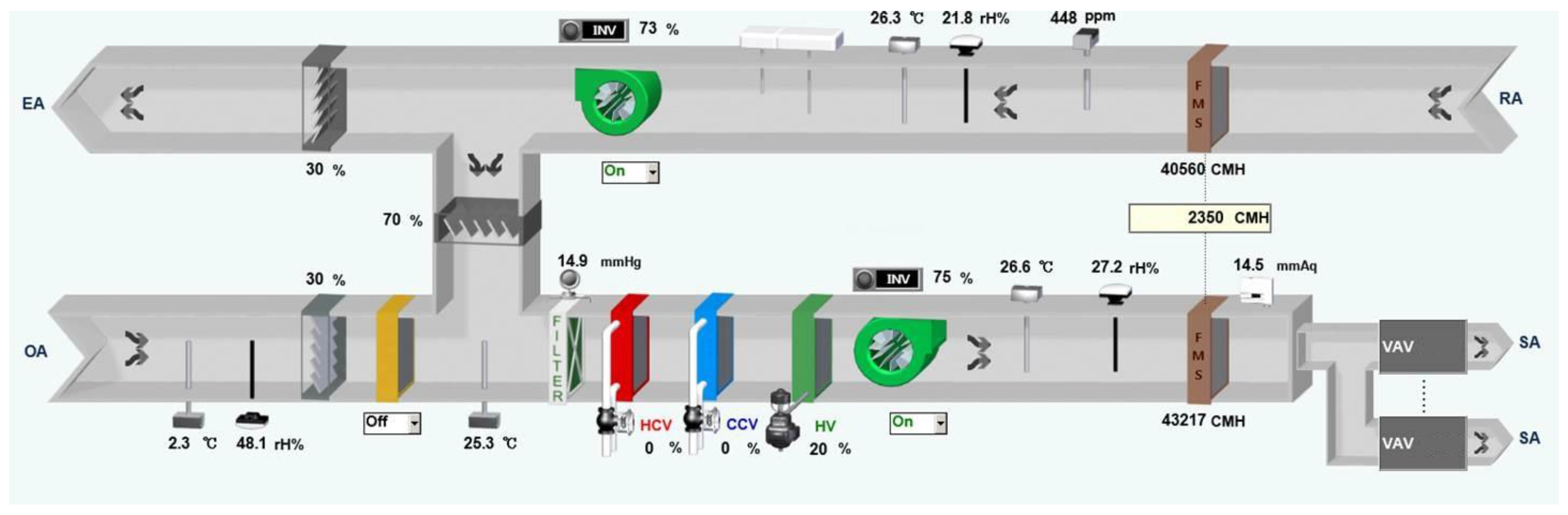
The case study is a fifteen-story hospital with six basement floors. The building is about 8600 m2 and approximately 80 m high. Figure 2 shows the typical organization of AHUs in patient rooms. An AHU consists of a chilled water cooling coil, steam heating coil, two fans, filters, dampers, and sensors. Hospital AHUs require more components than AHUs serving other types of buildings [21]. Table 1 shows the specification of the sensors for temperature and relative humidity. By using sensors mounted onto the AHU and ducts, the variables listed below were monitored (as shown in Figure 3) and the data was recorded by an interval period specified by the user.
The variables that were monitored include:
- Temperature (indoor air, outdoor air, supply air, return air, mixed air)
- Relative humidity (indoor air, outdoor air, supply air, return air)
- Air flow rate (supply air, return air)
- Pressure difference
- Coil valve opening ratio (heating, cooling)
- Indoor carbon dioxide
The data collection period was one year (from December 2015 to November 2016), with a measurement interval of an hour. In order to develop a suitable predictive model, it is important to select appropriate input data. A variety of input variables such as outdoor air temperature (OAT), mixed air temperature (MAT), return air temperature (RAT), and others which were monitored in the AHU, were used to develop a predictive model for SAT output. The data set was normalized by scaling data between 0 and 1.
Input variables, output variables, statistical indices, and data sets used in the existing literature were scrutinized and are summarized in Table 2. As shown in Table 2, data collected from measurements or from simulation programs were used to develop the predictive model. Mostly, input variables were outdoor air, supply air, indoor temperature, and humidity, all of which are measurable. Using this data, energy demand, room temperature, and relative humidity can be derived as outputs. This current study examined various methods to generate proper input variables.
As displayed in Table 2, statistical indicators were used to compare predicted values and actual values. The following statistical indicators were used: CV (coefficient of variation), mean square error (MSE), mean absolute error (MAE), root mean square error (RMSE), and coefficient of determination (r2). The present study used MSE, RMSE, and CVRMSE in order to assess and verify the results of the predictive model.
MSE means the standard error value and uses the measure of fitness for predictive values. The neural network algorithm seeks to minimize this MSE [6].
where, is the predicted value, is the actual value, is the number of data.
The prediction accuracy was also measured by the root mean square error (RMSE). RMSE is a frequently used measure of the differences between a model’s predicted values and the actual values. It follows Equation (2):
The CV (Coefficient of Variation) of the RMSE is a non-dimensional measure calculated by dividing the RMSE by the mean value of the actual temperature. Using CVRMSE makes it easier to determine the error range. The closer its value gets to 0%, the higher the accuracy.
The R program was used to predict the SAT of AHUs in this current study. R is a statistical tool that has a programming language built in. It can be used for a wide range of statistical analyses [22,23,24]. R offers many linear and nonlinear statistical models, classical statistical tests, time series analysis, classification, clustering, and graphical techniques. Therefore, it is very extensible. In addition, R is an analytical tool that supplies statistics and visualizations for language and the development environment. It can also provide statistical techniques, modeling, new data mining approaches, simulations, and numerical analysis methods [25].
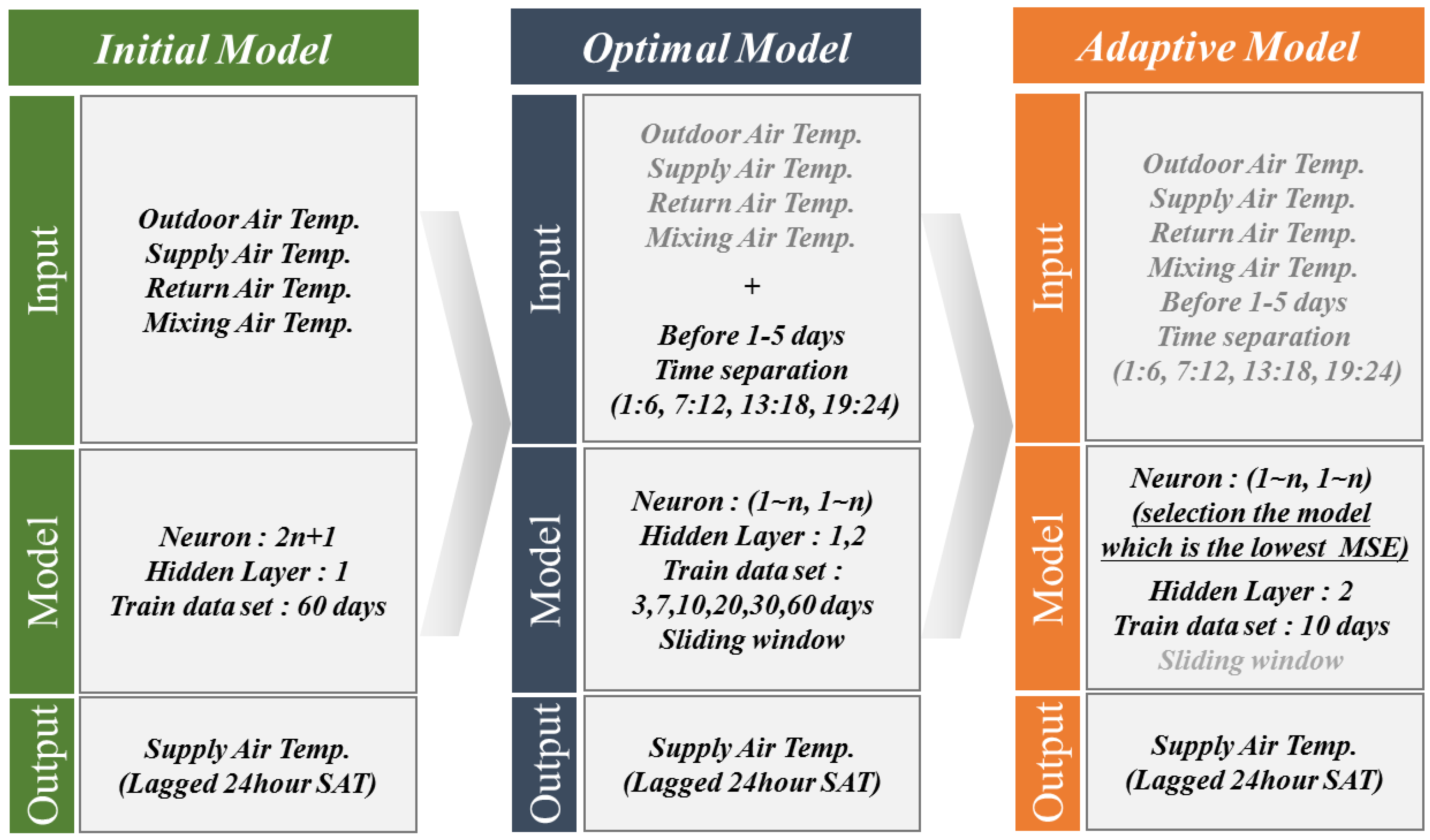
2.3. Initial Model
The process of finding an optimal predictive model is shown in Figure 4. The figure on the left shows the initial model. To predict the SAT of the AHU, operation data such as OAT, SAT, RAT, and MAT were selected as input variables for the initial model.
Data from the monitored AHU systems were collected only up to the present time. To predict the SAT for the future 24 h, input variables for the future 24 h are needed. However, there was no future input data. Therefore, time-lagged 24 h SAT (lag 24 SAT) should be considered as output in order to estimate SAT for the future 24 h. The lag 24 SAT was included as output and trained itself to estimate. Therefore, 24 h data collected from existing SAT data was used as lag 24 SAT data. The lag 24 SAT were collections of previous 24 h data.
Predicting results should be SAT(t + 1), SAT(t + 2),…, SAT(t + 24). However, at the present time (t), known data is input variables such as (t), (t − 1), (t − 2),…, (t − n). By adding lag 24 SAT as output variables for 24 h, it is possible to predict SAT. In other words, input variables are: OAT (t = training period), SAT (t = training period), RAT (t = training period), and MAT (t = training period). All input values up to the present time (t) exist except for the lag 24 SAT for the recent 24 h. This makes the prediction possible. The current study used time-lagged output variables to develop a step-ahead prediction model [4,11,22].
Initial models consist of one hidden layer with nine neurons, where the number of neurons was 2n + 1 (n = the number of input variables). The number of neurons was inferred from the survey of exiting literature [26,27,28]. To validate the initial model, data from December 2015 to January 2016 was used as training data.
2.4. Optimal Model
The model in the middle of Figure 4 is the optimal model. The diagram explains the ANN architecture. Different configurations of the input variables, number of hidden layers, number of neurons, and training periods were tested in order to derive the optimal model.
Since the initial model’s results were not perfect, additional input variables were considered. In order to take SAT changes occurring in previous days into consideration, a model with five more input variables was created. The five extra variables were collections of previous SAT from day 1 to day 5. Moreover, four additional input variables (dawn, morning, afternoon, and evening) were included. These four variables were used to divide 24 h. These variables were referred to the time series analysis method. The performance of the prediction was analyzed by adding the input variables mentioned above.
The optimal model positioned a different number of hidden layers and neurons in order to check the accuracy of the prediction. The number of hidden layers was one or two. The number of neurons was increased from one to the number of input variables. Training times were: day 3, day 7, day 10, day 20, day 30, and day 60 because the amount of training data could affect the accuracy of the model [29].
An ANN can periodically be retrained using an augmented data set filled with new measurements. This method is also referred to as accumulative training. It can help an ANN to recognize daily and seasonal trends in predicted values. However, one drawback is that a large amount of data continuously accumulating, may become too difficult to control. Larger amounts of data mean longer training times for the ANN. Data volume can be set so that the oldest data is removed as new measurements are added. This can be achieved using a graph and periodically sliding a time window across a time series of measurements when choosing training data. In comparison with accumulative training, the sliding window technique can provide better results for real measurements [22]. The current study used the sliding window training technique.
The present study identified the optimal model by allocating the same number of neurons to the number of hidden layers. In this case, input variables were 13 and hidden layers were 2. Therefore, neuron values (number of neurons in the first hidden layer, number of neurons in the second hidden layer) were (1,1), (2,1), (2,2), (3,1),…, (13,13), resulting in a total of 91 models.
2.5. Adaptive Model
Basic ANN architecture was created through the process of finding the optimal model. More efficient models such as an adaptive model had to be considered. Configuration of the adaptive model is shown on the right of Figure 4.
In order to find the adaptive model, a test data set was set up to examine the accuracy of the prediction. However, when actually conducting predictions, there were no test data set. It was unclear how well the prediction matched the actual value. Learning period data changed continuously because hourly data was stored. The optimal model as described in Section 2.4 might lower the prediction accuracy. To overcome this issue, data from the previous 12 h of predicted values for 24 h was used as test data and models with various number of neurons were tested again to achieve better prediction performance. A total of 91 models with neuron numbers of (1,1), (2,1), (2,2), (3,1),…, and (13,13) were analyzed to find the most appropriate model. Outputs of these models were compared with the 12-hour test data and the model with the lowest MSE value was selected as an adaptive model.
As training data changed, an adaptive model was developed to improve the prediction performance by selecting the best model among 91 models using various neuron numbers.
For validation of the final adaptive model, AHU data from another building was used. The data measuring period was from 6 March 2017 to 23 April 2017 for each hour.
3. Results
3.1. Initial Model
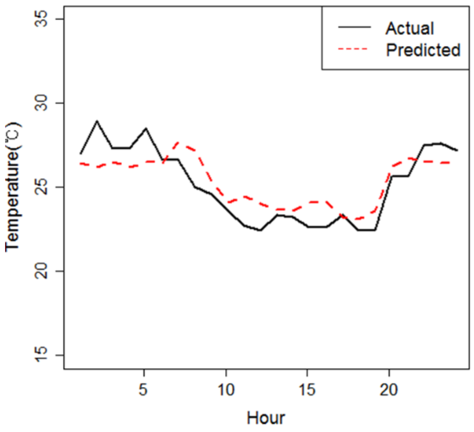
Results of the comparison between predicted temperature and actual temperature derived from the initial model are shown in Figure 5. The predicted temperature followed a pattern similar to the actual temperature, with an MSE of 1.54, RMSE of 1.2 °C, and CVRMSE of 5%. Although the accuracy error was large, the initial model showed great potential in predicting SAT.
3.2. Optimal Model
3.2.1. Kinds of Input Variables
The basic model had two hidden layers with the same input variables as the initial model. In order to develop an optimal model, the prediction performance of models with added input variables was evaluated. The before model included five added variables—from before 1 day to before 5 days. The other model was called the hour model. It had four added input variables derived by dividing a 24 h period into dawn, morning, afternoon, and night.
The composition and results of each model are summarized in Table 3. Since the basic model had four inputs, according to the number of neurons with two hidden layers at (1,1), (2,1), (2,2), (3,1),…, (4,4), there were a total of 10 models. Among these 10 models, the basic model with neuron number (4,3) showed an MSE of 1.02, RMSE of 1.01 °C, and CVRMSE of 4.0%. The hour model with 13 input variables and two hidden layers had an MSE of 0.61, RMSE of 0.78 °C, and CVRMSE of 3.1%. These results indicate that the predictive performance is better when more input variables are involved in the model.
Results of comparison between actual temperature and predicted temperature among the basic model, before model, and hour model are shown in Figure 6. These are images that were expressed in program R. The predicted temperature showed a distribution pattern similar to the actual temperature. The difference between predicted temperature and the actual temperature ranged from 0.8 °C to 1.0 °C.
3.2.2. Number of Hidden Layers
As described in Section 3.2.1, the number of input variables was determined to be 13. Since the hour model had two hidden layers, 13 neurons were considered in one hidden layer. Results of the prediction performance of 13 models are summarized in Table 4. RMSE values ranged from 1.0 °C to 2.1 °C. CVRMSE values ranged from 3.9% to 8.3%. The model with nine neurons showed an MSE of 1.0, RMSE of 1.0 °C, and CVRMSE of 3.9%. It had the highest prediction performance among these 13 single hidden layer models.
When there were two hidden layers, the number of neurons was 13 for each hidden layer. A total of 91 models were obtained. RMSE values ranged from 0.8 °C to 22.7 °C. The model with the number of neurons of (5,2) showed an MSE of 0.6, RMSE of 0.8 °C, and CVRMSE of 3.1%. Therefore, the model with two hidden layers has a better prediction performance than the model with one hidden layer.
3.2.3. Period of Training Data Set
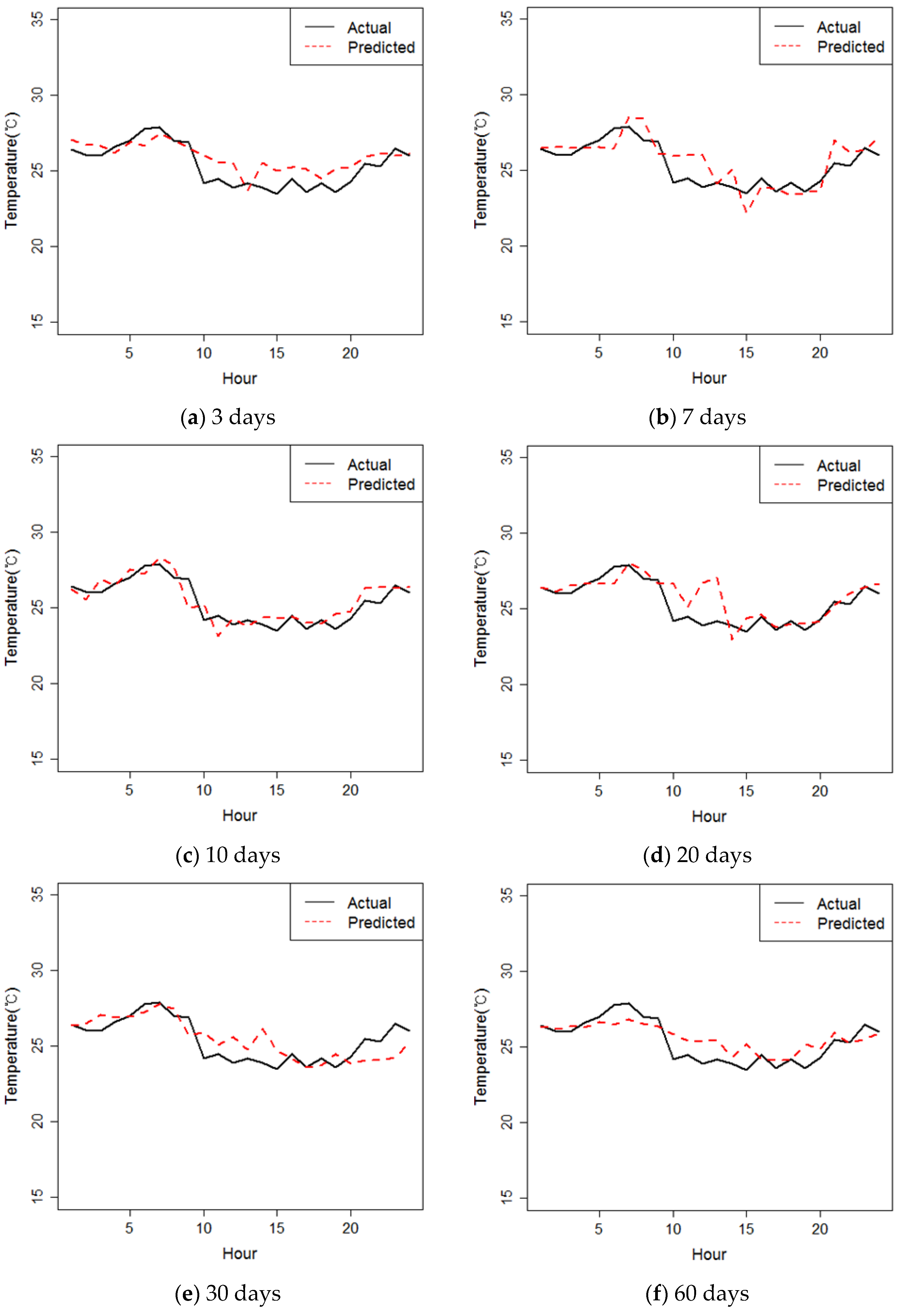
Based on the results shown above, the number of hidden layers and neurons of the optimal model were determined to be 2 and (5,2), respectively. Results for the predictive performance of models with various time periods of data training are shown in Table 5. The optimal duration was 10 days. It had an MSE of 0.59, RMSE of 0.77 °C, and CVRMSE of 3.0%. On the other hand, the MSE showed an increase when the learning period was much longer (20 days and 30 days). The learning period of 60 days also had a low MSE value at 0.77. However, data for the learning period of 60 days took much longer to obtain results. The longer the time period used for training data, the longer the processing time to obtain result. In the present study, the data training period was set to 10 days for the optimal model.
Graphs of actual temperature and predicted temperature by each time period of data training are shown in Figure 7.
3.3. Fixed Optimal Model
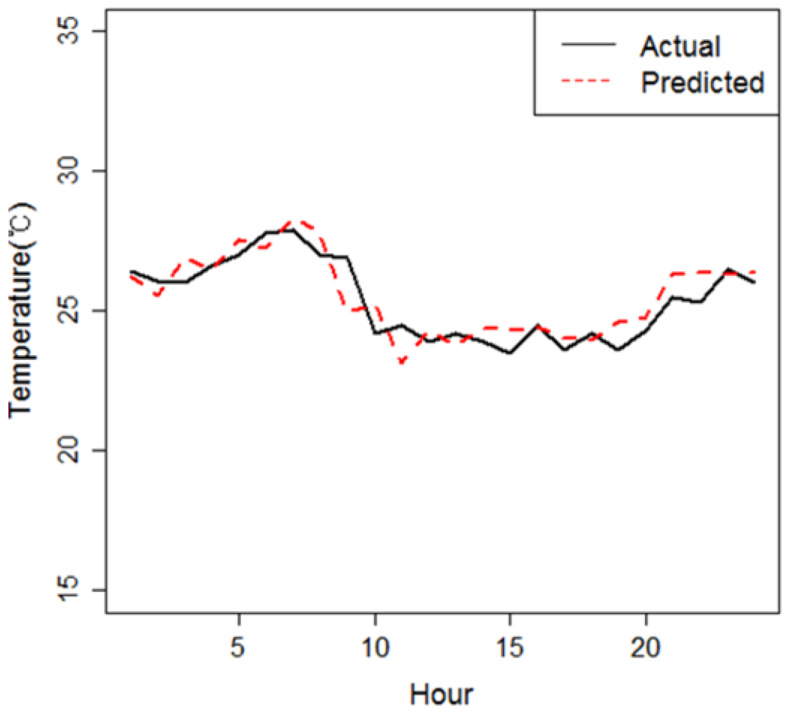
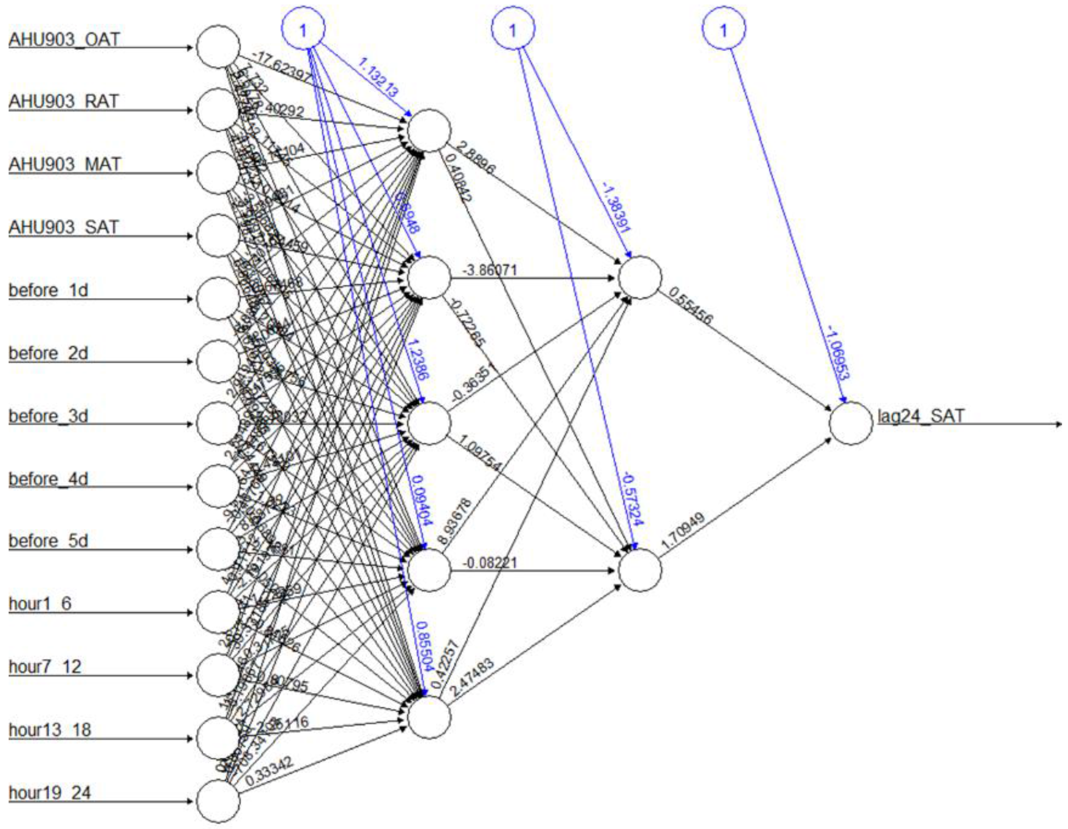
The optimal model consisted of 13 input variables, neuron numbers of (5,2), two hidden layers, and a learning period of 10 days. It had an MSE of 0.59, RMSE of 0.77 °C, and CVRMSE of 3.0%. Results from the comparison between actual temperature and predicted temperature using the optimal model are shown in Figure 8. The structure of the model expressed in the R program is shown in Figure 9. The weight of each connection in the optimal model is also shown in Figure 9. Black lines represent the connection between each layer and weights of each connection. Blue lines represent the bias term added in each step.
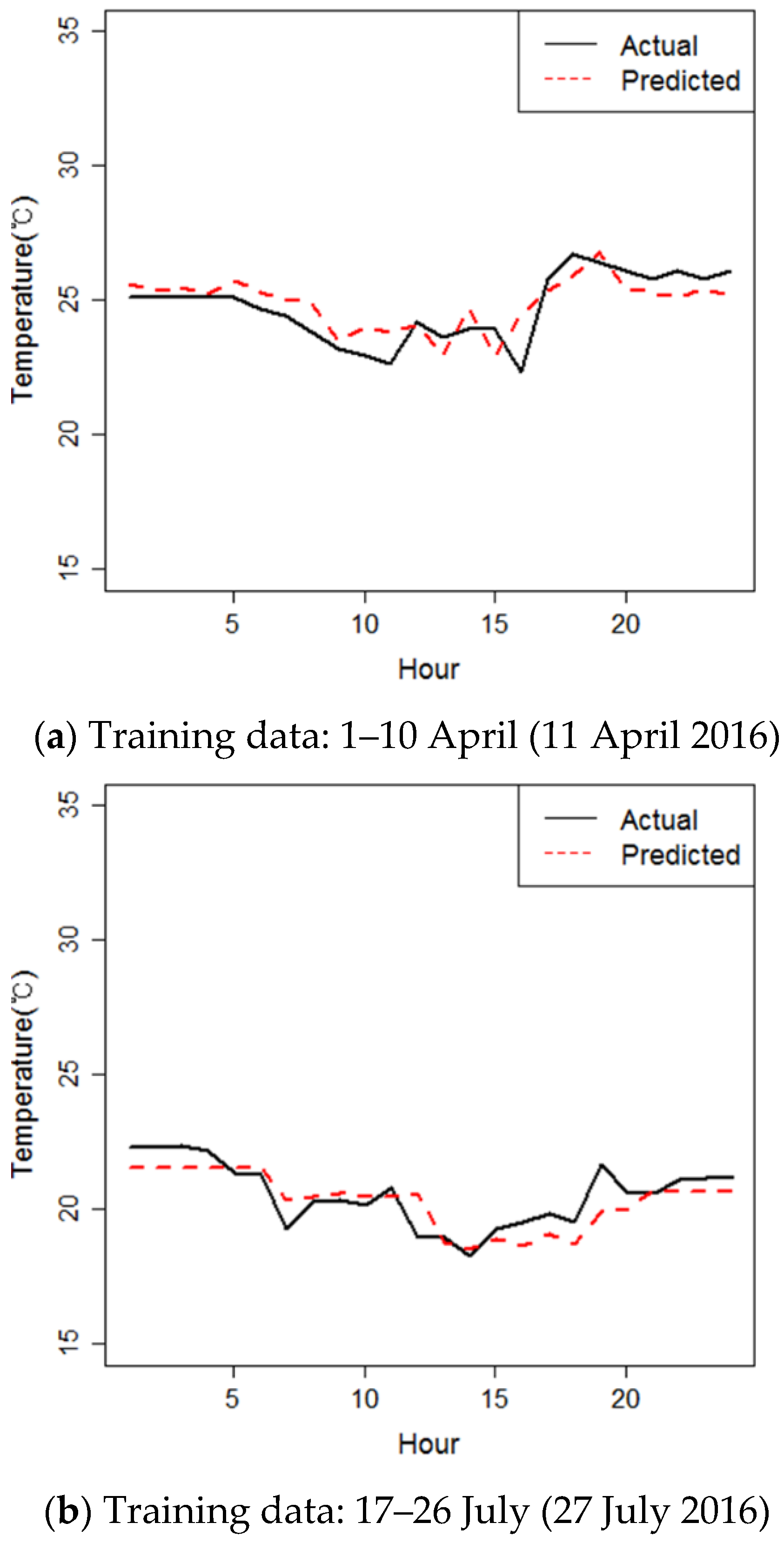
3.4. Final Adaptive Model
Results of the comparison between actual temperature and predicted temperature using the developed adaptive model are shown in Figure 10. The predicted temperature was learned at different time periods by using the adaptive model. Model (a) had (13,9) neurons. Training data used for model (a) was obtained from April 1 to April 10. It had an MSE of 0.66, RMSE of 0.81 °C, and CVRMSE of 3.3%. Model (b) had (5,5) neurons. Its training data was obtained from July 17 to July 26. It had an MSE of 0.52, RMSE of 0.72 °C, and CVRMSE of 3.5%.
It could be seen that the model changed instantaneously depending on the training data. Therefore, it was an adaptive model through learning and seeking a model with the lowest MSE.
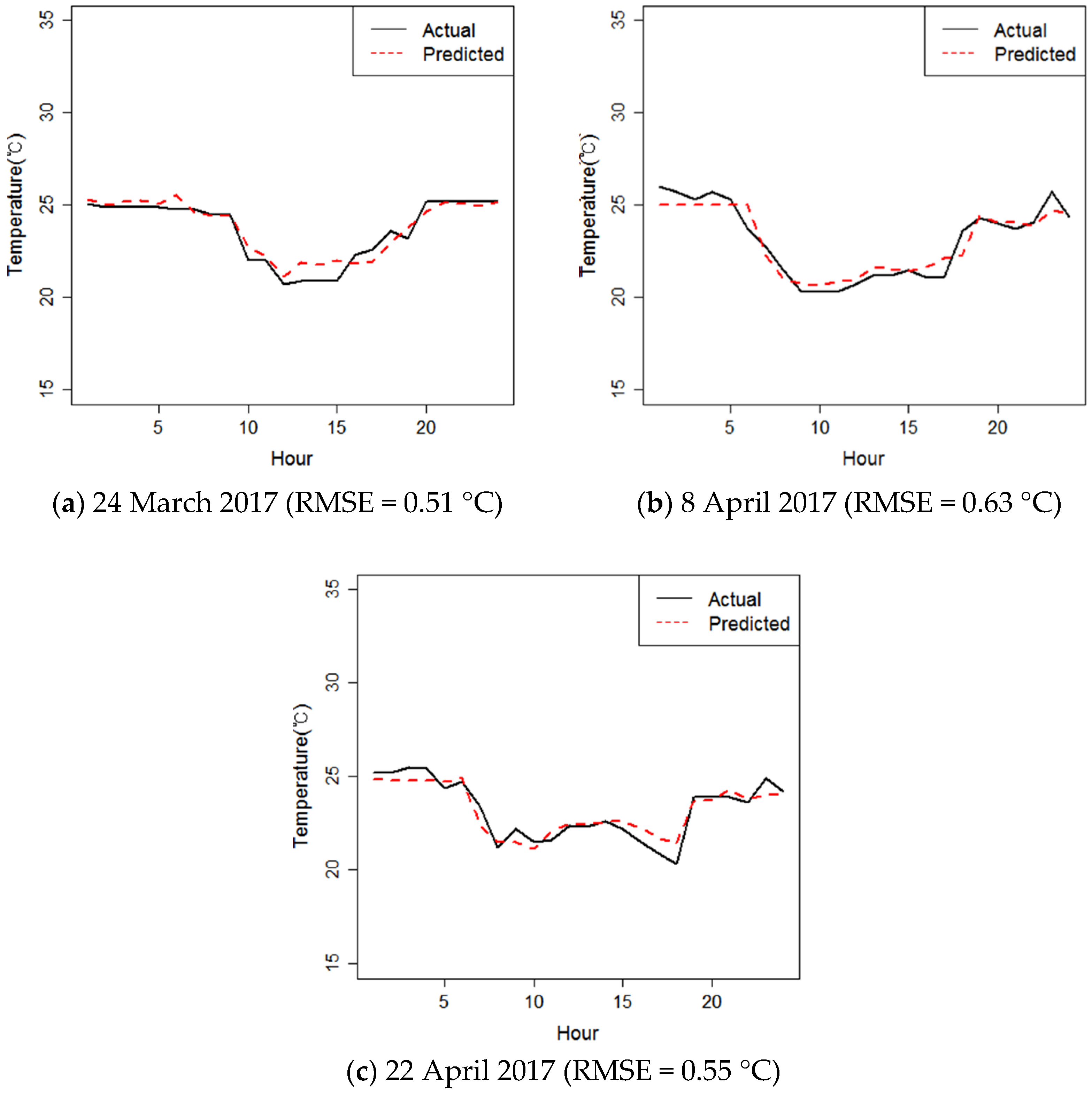
3.5. Validation of the Adaptive Model
By using another building’s AHU data, the predictive performance of the adaptive model was verified. The actual temperature and predicted temperature are shown in Figure 11. In Figure 11, (a) predicts the SAT on 24 March. The difference between the predicted value and the actual value is MSE = 0.26, RMSE = 0.51 °C, and CV = 2.2%; (b,c) with a RMSE of 0.63°C and 0.55 °C, respectively, also show a better prediction performance than the original case study. Predicted temperature distribution is similar to actual temperature.
4. Discussion and Conclusions
This study predicted the SAT of an AHU using an ANN. In addition, a model with good predictive performance was developed using an initial model, an optimal model, and an adaptive model.
The potential of SAT prediction was found through the initial model. Parameters and number of input variables are important in the process of finding an optimal model. The hour model with various input variables showed a 25% improvement in prediction performance than the basic model which used temperature measured within the AHU.
A total of 91 models with two hidden layers were tested. The prediction performance was improved 20% (RMSE-based) when the number of hidden layers was two instead of one.
Two hidden layers and (5,2) neurons were selected for the optimal model. It is difficult to determine the number of hidden layers and the number of neurons [9]. The number of neurons should be made to correspond to the number of input and output variables and should also follow some simple rules [30]. Unfortunately, few studies have provided guidelines for selecting the best layer or neuron numbers. Therefore, factors such as the number of hidden layers and neurons should be determined based on the characteristics of the application and data [31].
Based on the results of performance using various periods for data learning, 10 days was determined to be the best for the optimal model developed in the present study. When the learning period was increased to 20 or 30 days, the MSE value increased. Therefore, it is important to review the length of the data learning period according to data characteristics. When the learning period was increased to 60 days, the prediction performance was better than that with learning period of 20 or 30 days. However, such a long learning period was ultimately inefficient because its execution took a much longer time [32]. Even though a learning period of 3 days also showed good results, such a short time period might not completely capture the trends for the predicted values [22].
The optimal model developed in this current study is a model that can use recently collected data. It was developed by using a data training approach with a sliding window method rather than using an accumulative data method. Applying the sliding window technique makes it possible to maintain a training data set of a relatively small and constant size and retrain it quickly. However, annual and seasonal changes may not be accurately reflected in the prediction results.
Although the optimal model was developed, learning data changes over time. A fixed optimal model dependent on changing training data does not show uniformly good prediction performance results.
In conclusion, an adaptive model was developed by selecting a model with the lowest MSE. A total of 91 models were evaluated after setting up a 12-h test set at every prediction. The adaptive model can learn from training data that changes in real time. It seeks the model that has the best prediction performance. The prediction performance of the adaptive model is similar to that of the optimal model. However, it has the advantage of being able to actively cope with changing training data.
Acknowledgments
This research was supported by Basic Science Research Program through the National Research Foundation of Korea (NRF) funded by the Ministry of Education (NRF-2015R1D1A1A01057928).
Author Contributions
Goopyo Hong initiated the research idea and wrote the manuscript. Byungseon Sean Kim supervised the study and provided advice on the data analysis.
Conflicts of Interest
The authors declare no conflict of interest.
References
- Zhao, H.-X.; Magoulès, F. A review on the prediction of building energy consumption. Renew. Sustain. Energy Rev. 2012, 16, 3586–3592. [Google Scholar] [CrossRef]
- Ruano, A.E.; Crispim, E.M.; Conceição, E.Z.E.; Lúcio, M.M.J.R. Prediction of building's temperature using neural networks models. Energy Build. 2006, 38, 682–694. [Google Scholar] [CrossRef]
- ASHRAE. ASHRAE Handbook Fundamental—Chapter 19 Energy Estimating and Modeling Method; ASHRAE: Atlanta, CA, USA, 2013. [Google Scholar]
- Mustafaraj, G.; Lowry, G.; Chen, J. Prediction of room temperature and relative humidity by autoregressive linear and nonlinear neural network models for an open office. Energy Build. 2011, 43, 1452–1460. [Google Scholar] [CrossRef]
- Ferdyn-Grygierek, J.; Grygierek, K. Multi-Variable Optimization of Building Thermal Design Using Genetic Algorithms. Energies 2017, 10, 1570. [Google Scholar] [CrossRef]
- Abdullatif, E.; Ben-Nakhi, M.A.M. Energy conservation in buildings through efficient AC control using neural networks. Appl. Energy 2002, 73, 5–23. [Google Scholar]
- Kang, I.-S.; Lee, H.-E.; Park, J.-C.; Moon, J.-W. Development of an Artificial Neural Network Model for a Predictive Control of Cooling Systems. KIEAE J. 2017, 17, 69–76. [Google Scholar] [CrossRef]
- Baik, Y.K.; Moon, J.W. Development of Artificial Neural Network Model for Predicting the Optimal Setback Application of the Heating Systmes. KIEAE J. 2016, 16, 89–94. [Google Scholar] [CrossRef]
- Yang, I.-H.; Kim, K.-W. Prediction of the time of room air temperature descending for heating systems in buildings. Build. Environ. 2004, 39, 19–29. [Google Scholar] [CrossRef]
- Neto, A.H.; Fiorelli, F.A.S. Comparison between detailed model simulation and artificial neural network for forecasting building energy consumption. Energy Build. 2008, 40, 2169–2176. [Google Scholar] [CrossRef]
- Kreider, J.F.; Blanc, S.L.; Kammerud, R.C.; Curtiss, P.S. Operational data as the basis for neural network prediction of hourly electrical demand. ASHRAE Trans. 1997, 103, 926. [Google Scholar]
- Underwood, C.P. HVAC Control Systems Modelling Analysis and Design; Taylor and Francis: London, UK; New York, NY, USA, 1999. [Google Scholar]
- Miller, R.; Seem, J. Comparison of artificial neural networks with traditional methods of predicting return time from night or weekend setback. ASHRAE Trans. 1991, 97 Pt 1, 500–508. [Google Scholar]
- Nakahara, N.; Zheng, M.; Pan, S.; Nishitani, Y. Load Prediction for Optimal Thermal Storage—Comparison of Three Kinds of Model Application. In Proceedings of the IBPSA Building Simulation Conference, Kyoto, Japan, 13–15 September 1999; pp. 519–526. [Google Scholar]
- Park, D.H.; N, H.M.; Chung, H.G.; Yang, I.H. Analysis of Energy Saving Effect of Optimal Start Stop with ANN on Heating and Cooling System; Korean Journal of Air-Conditioning and Refrigerating Engineering; SAREK: Seoul, Korea, 2014. [Google Scholar]
- Nabil Nassif, P.E. Modeling and optimization of HVAC systems using artificial intelligence approaches. ASHRAE Trans. 2012, 118, 133. [Google Scholar]
- Kusiak, A.; Li, M.; Zhang, Z. A data-driven approach for steam load prediction in buildings. Appl. Energy 2010, 87, 925–933. [Google Scholar] [CrossRef]
- Massie, D.D.; Curtiss, P.S.; Kreider, J.F.; Dodier, R. Predicting Central Plant HVAC Equipment Performance Using Neural Networks Laboratory System Test Results. ASHRAE Trans. 1998, 104, 221. [Google Scholar]
- Yao, Y.; Yu, Y. Modeling and Control in Air Conditioning Systems; Springer: Berlin/Heidelberg, Germany, 2016. [Google Scholar]
- Tso, G.K.F.; Yau, K.K.W. Predicting electricity energy consumption: A comparison of regression analysis, decision tree and neural networks. Energy 2007, 32, 1761–1768. [Google Scholar] [CrossRef]
- ASHRAE. HVAC Design Manual for Hospitals and Clinics, 2nd ed.; ASHRAE: Atlanta, CA, USA, 2013. [Google Scholar]
- Yang, J.; Rivard, H.; Zmeureanu, R. On-line building energy prediction using adaptive artificial neural networks. Energy Build. 2005, 37, 1250–1259. [Google Scholar] [CrossRef]
- Jeannette, E.; Curtiss, P.S.; Assawamartbunlue, K.; Kreider, J.F. Experimental results of a predictive neural network HVAC controller. ASHRAE Trans. 1998, 104, 192. [Google Scholar]
- The R Project for Statistical Computing. Available online: https://www.r-project.org/ (accessed on 6 February 2017).
- Kim, S.H.; S, H.S.; Son, S.H. A Study on Large-Scale Traffic Information Modeling using R. J. KIISE 2015, 41, 151–157. [Google Scholar]
- Hecht-Nielsen, R. Theory of the Back propagation Neural Network. In International Joint Conference on Neural Networks; IEEE: Washington, DC, USA, 1989. [Google Scholar]
- Yang, I.-H.; Yeo, M.-S.; Kim, K.-W. Application of artificial neural network to predict the optimal start time for heating system in building. Energy Convers. Manag. 2003, 44, 2791–2809. [Google Scholar] [CrossRef]
- Argiriou, A.A.; Bellas-Velidis, I.; Kummert, M.; André, P. A neural network controller for hydronic heating systems of solar buildings. Neural Netw. 2004, 17, 427–440. [Google Scholar] [CrossRef] [PubMed]
- Wang, S.; Jin, X. Model-based optimal control of VAV air-conditioning system using genetic algorithm. Build. Environ. 2000, 35, 471–487. [Google Scholar] [CrossRef]
- Barga, R.; Fontama, V.; Tok, W.H.; Cabrera-Cordon, L. Predictive Analytics with Microsoft Azure Machine Learning; Apress: Berkley, CA, USA, 2016. [Google Scholar]
- Zurada, J.M. Introduction to Artificial Neural Systems; West Publishing Company: West St. Paul, MN, USA, 1992; ISBN 10: 0314933913. [Google Scholar]
- Anstett, M.; Kreider, J. Application of artificial neural networks to commercial energy use prediction. ASHRAE Trans. 1993, 99, 505–517. [Google Scholar]
Figure 1.
Typical feed-forward network. (OA: Outdoor air, RA: Return air, and SA: Supply air).
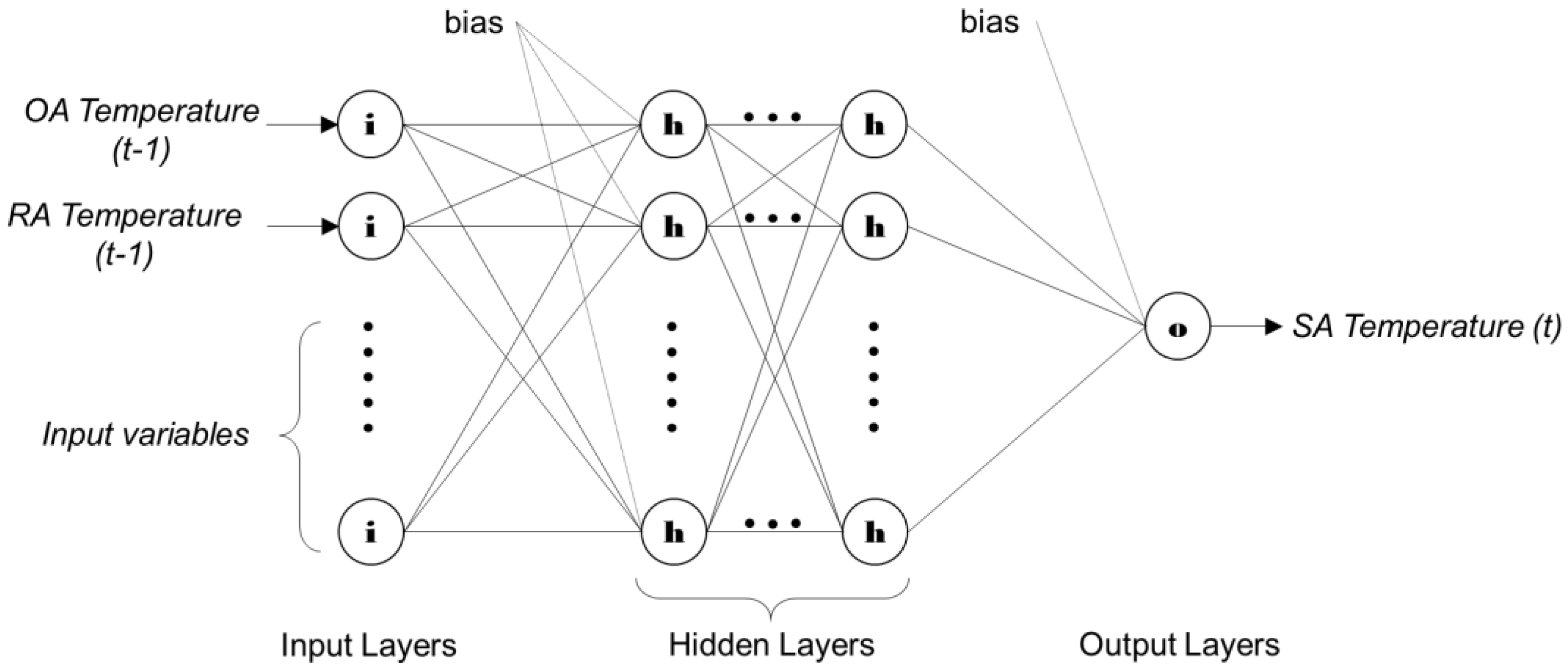
Figure 2.
Schematic of case study air-handling unit (AHU). (EA: Exhaust air).

Figure 3.
Monitoring of the case study AHU.

Figure 4.
Evolving model process and artificial neural network (ANN) architecture.

Figure 5.
Comparison of actual temperature and predicted temperature using the initial model (24 February 2016).
Figure 5.
Comparison of actual temperature and predicted temperature using the initial model (24 February 2016).

Figure 6.
Comparison of actual and predicted temperature by kinds of input variables (20 February 2016).
Figure 6.
Comparison of actual and predicted temperature by kinds of input variables (20 February 2016).
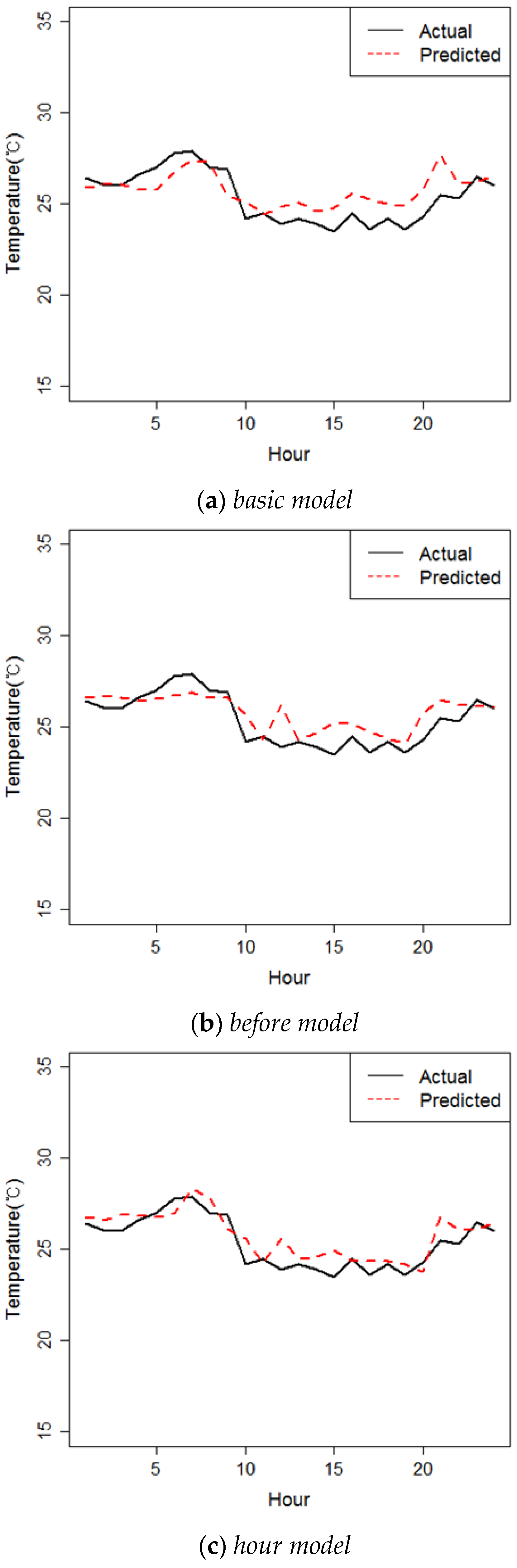
Figure 7.
Comparison of actual temperature and predicted temperature by time period of data training (20 February 2016).
Figure 7.
Comparison of actual temperature and predicted temperature by time period of data training (20 February 2016).

Figure 8.
Comparison of actual and predicted temperatures using the optimal model (20 February 2016).
Figure 8.
Comparison of actual and predicted temperatures using the optimal model (20 February 2016).

Figure 9.
Structure of optimal model using R.

Figure 10.
Comparison between actual and predicted temperature using developed adaptive model.

Figure 11.
Comparison between actual and predicted temperature for validation.


Table 1.
Specification of Temperature and Humidity Sensors in the AHU.
| Feature | Temperature Sensor | Humidity Sensor |
|---|---|---|
| Model | HTE200B12E1 | HRH200A02 |
| Range | −40 °C–70 °C | 0–100% RH |
| Accuracy | ±0.2 °C at 25 °C | ±2% RH |
Table 2.
Input and output variables from the literature survey.
| Authors | Input Variables | Output | Statistical Indices | Data Set |
|---|---|---|---|---|
| Jin Yang et al. [22] | Outdoor dry-bulb Temperature Outdoor wet-bulb Temperature Temperature of water leaving the chiller | Chiller electric demand | CV, RMSE | Synthetic data (DOE 2.1E software) |
| Mustafaraj et al. [4] | Outside temperature Outside relative humidity Supply air temperature Supply air relative humidity Supply air flow rate Chilled water temperature Hot water temperature Room Carbon dioxide concentration | Room temperature Room relative humidity | MSE, MAE, G (goodness of fit) r2 | Measurement data (summer season) |
| Ruano et al. [2] | Outside solar radiation Outside air temperature Outside relative humidity | Room temperature | RMSE | Measurement data |
| Yang et al. [9] | Room air temperature Variation rate of room air temperature Outdoor air temperature Variation rate outdoor air temperature | The decent time of room air temperature | r2 | Simulation data |
| Krider et al. [18] | Outdoor Temperature Evaporator Inlet temperature Evaporator Exit temperature Ice Valve | Chiller thermal load & power usage | RMSE, CV(RMSE) | By operating a full-scale HVAC laboratory |
| Jeannette et al. [23] | Hot water supply temperature Boiler outlet temperature Boiler stage controller output Three-way valve controller output | Hot water supply temperature, Boiler outlet temperature | Coefficient of variation (CV) | Measurement data |
Table 3.
Models by kinds of input variables and performance results.
| Parameter | Basic Model | Before Model | Hour Model |
|---|---|---|---|
| Number of inputs | 4 | 9 | 13 |
| Hidden layer/Neurons | 2/(1,1), (2,1), (2,2), (3,1),…, (4,4) | 2/(1,1), (2,1), (2,2), (3,1),…, (9,9) | 2/(1,1), (2,1), (2,2), (3,1),…, (13,13) |
| MSE | 1.02 | 0.87 | 0.61 |
| RMSE | 1.01 °C | 0.93 °C | 0.78 °C |
| CVRMSE | 4.0% | 3.7% | 3.1% |
Table 4.
Model performance according to the number of neurons with one hidden layer.
| Neuron | MSE | RMSE | CVRMSE |
|---|---|---|---|
| 1 | 1.0 | 1.0 | 4.0% |
| 2 | 1.9 | 1.4 | 5.5% |
| 3 | 1.4 | 1.2 | 4.7% |
| 4 | 1.3 | 1.2 | 4.5% |
| 5 | 1.8 | 1.3 | 5.2% |
| 6 | 1.3 | 1.1 | 4.4% |
| 7 | 4.4 | 2.1 | 8.3% |
| 8 | 1.5 | 1.2 | 4.8% |
| 9 | 1.0 | 1.0 | 3.9% |
| 10 | 1.1 | 1.0 | 4.1% |
| 11 | 3.4 | 1.8 | 7.3% |
| 12 | 2.2 | 1.5 | 5.8% |
| 13 | 1.5 | 1.2 | 4.8% |
Table 5.
Prediction performance according to time period used for data training.
| Indicators | 3 Days | 7 Days | 10 Days | 20 Days | 30 Days | 60 Days |
|---|---|---|---|---|---|---|
| MSE | 0.95 | 1.03 | 0.59 | 1.16 | 1.12 | 0.77 |
| RMSE (°C) | 0.97 | 1.01 | 0.77 | 1.08 | 1.06 | 0.88 |
| CVRMSE | 3.8% | 4.0% | 3.0% | 4.2% | 4.2% | 3.5% |
© 2018 by the authors. Licensee MDPI, Basel, Switzerland. This article is an open access article distributed under the terms and conditions of the Creative Commons Attribution (CC BY) license (http://creativecommons.org/licenses/by/4.0/).
Share and Cite
MDPI and ACS Style
Hong, G.; Kim, B.S. Development of a Data-Driven Predictive Model of Supply Air Temperature in an Air-Handling Unit for Conserving Energy. Energies 2018, 11, 407. https://doi.org/10.3390/en11020407
AMA Style
Hong G, Kim BS. Development of a Data-Driven Predictive Model of Supply Air Temperature in an Air-Handling Unit for Conserving Energy. Energies. 2018; 11(2):407. https://doi.org/10.3390/en11020407
Chicago/Turabian StyleHong, Goopyo, and Byungseon Sean Kim. 2018. "Development of a Data-Driven Predictive Model of Supply Air Temperature in an Air-Handling Unit for Conserving Energy" Energies 11, no. 2: 407. https://doi.org/10.3390/en11020407
Note that from the first issue of 2016, this journal uses article numbers instead of page numbers. See further details here.