Bayesian Energy Measurement and Verification Analysis


1
Centre for New Energy Systems, University of Pretoria, Pretoria 0002, South Africa
2
Department of Industrial and Systems Engineering, University of Pretoria, Pretoria 0002, South Africa
*
Author to whom correspondence should be addressed.
Energies 2018, 11(2), 380; https://doi.org/10.3390/en11020380
Submission received: 5 December 2017
/
Revised: 12 January 2018
/
Accepted: 18 January 2018
/
Published: 6 February 2018
(This article belongs to the Special Issue Bayesian Building Energy Modeling)
Abstract
:Energy Measurement and Verification (M&V) aims to make inferences about the savings achieved in energy projects, given the data and other information at hand. Traditionally, a frequentist approach has been used to quantify these savings and their associated uncertainties. We demonstrate that the Bayesian paradigm is an intuitive, coherent, and powerful alternative framework within which M&V can be done. Its advantages and limitations are discussed, and two examples from the industry-standard International Performance Measurement and Verification Protocol (IPMVP) are solved using the framework. Bayesian analysis is shown to describe the problem more thoroughly and yield richer information and uncertainty quantification results than the standard methods while not sacrificing model simplicity. We also show that Bayesian methods can be more robust to outliers. Bayesian alternatives to standard M&V methods are listed, and examples from literature are cited.
1. Introduction
This study argues for the adoption of the Bayesian paradigm in energy Measurement and Verification (M&V) analysis. As such, no new Bayesian methods will be developed. Instead, the advantages, limitations, and application of the Bayesian approach to M&V will be explored. Since the focus is on application, a full explanation of the underlying theory of the Bayesian paradigm will not be given. Readers are referred to Sivia and Skilling [1] or Kruschke [2] for a basic introduction, or von der Linden et al. [3] or Gelman et al. [4] for more complete treatments.
The argument made below is not that current methods are completely wrong or that the Bayesian paradigm is the only viable option, but that the field can benefit from a increased adoption of Bayesian thinking because of its ease of implementation and accuracy of the results.
This paper is arranged as follows. After discussing the background of current M&V analysis methods and the opportunities for improvement in Section 1.1, the Bayesian paradigm is introduced and its practical benefits and some caveats are discussed in Section 2. Section 3 offers two well-known examples and their Bayesian solutions. We also discuss robustness and hierarchical modelling. Section 4 gives a reference list of Bayesian solutions to common M&V cases.
1.1. Background
M&V is the discipline in which the savings from energy efficiency, demand response, and demand-side management projects are quantified [5], based on measurements and energy models. A large proportion of such M&V studies quantify savings for building projects, both residential and commercial. The process usually involves taking measurements or sampling a population to create a baseline, after which an intervention is done. The results are also measured, and the savings are inferred as the difference between the actual post-intervention energy use, and what it would have been, had no intervention taken place. These savings are expressed in probabilistic terms following the International Standards Organization (ISO) Guide to the Expression of Uncertainty in Measurement (GUM) [6]. M&V study results often form the basis of payment decisions in energy performance contracts, and the risk-implications of such studies are therefore of interest to decision makers.
The Bayesian option will not affect the foundational M&V methodologies such as retrofit isolation or whole facility measurement, but only the way the data are analysed once one of these methods has been decided upon.
M&V guidelines such as the International Performance Measurement and Verification Protocol (IPMVP) [5], the American Society of Heating, Refrigeration, and Air Conditioning Engineers (ASHRAE)’s Guideline 14 on Measurement of Energy, Demand, and Water Savings [7], or the United States Department of Energy’s Uniform Methods Project (UMP) [8], as well as most practitioners, use frequentist (or classical) statistics for analysis. Because of its popularity in the twentieth century, most practitioners are unaware that this is only one statistical paradigm and that its assumptions can be limiting. The term ‘frequentist’ derives from the method that equates probability with long-run frequency. For coin flips or samples from a production line, this assumption may be valid. However, for many events, equating probability with frequency seems strained because a large, hypothetical long-run population needs to be imagined for the probability-as-frequency-view to hold. Kruschke [2] gives an example where a coin is flipped twenty times and seven heads are observed. The question is then: what is the probability of the coin being fair? The frequentist answer will depend on the imagined population from which the data were obtained. This population could be obtained by “stopping after 20 flips”, but it could also be “stopping after seven heads” or “stopping after two minutes of flipping” or “to compare it to another coin that was flipped twenty times”. In each case, the probability that it is a fair coin changes, even though the data did not—termed incoherence [9]. In fact, the probabilities are dependent on the analyst’s intention. By changing his intention, he can alter the probabilities. This problem becomes even more severe in real-world energy savings inference problems with many more factors. The hypothetical larger population from which the energy use at a specific time on a specific day for a specific facility was sampled is difficult to imagine. That is not to say that a frequentist statistical analysis cannot be done, or be useful. However, it often does not answer the question that the analyst is asking, committing an “error of the third kind”. Analysts have become used to these ‘statistical’ answers (e.g., “not able to reject the null hypothesis”), and have accepted such confusion as part of statistics. For example, consider two mainstays of frequentist M&V: confidence intervals (CIs) and p-values. CIs are widely used in M&V to quantify uncertainty. According to Neyman, who devised these intervals, they do not convey a degree of belief, or confidence, as is often thought. Frequentist confidence intervals are produced by a method that yields an interval that contains the true value only in a specified percentage (say 90%) of cases [10]. This may seem like practically the same thing, but an explanation from most frequentist statistics textbooks will then seem very confusing. Consider Montgomery and Runger’s Applied Statistics and Probability for Engineers [11], under “Interpreting a Confidence Interval” (CI). They explain that, with frequentist CIs, one cannot say that the interval contains the true number with a probability of e.g., 90%. The interval either contains the value, or it does not. Therefore, the probability is either zero or one, but the analyst does not know which. Therefore, the interval cannot be associated with a probability. Furthermore, it is a random interval (emphasis theirs) because the upper and lower bounds of the interval are random variables.
Consider now the p-value. Because of the confusion surrounding this statistic, the American Statistical Association issued a statement regarding its use [12], in which they state that p-values neither signify probabilities of the hypothesis being true or false, nor are they probabilities that the result arose by chance. They go on to say that business (or policy) decisions should not be based on p-value thresholds. p-values do not measure effect sizes or result importances, and by themselves are not adequate measures of evidence.
Such statements by professional statisticians leave most M&V practitioners justifiably confused. It is not that these methods are invalid, but that they have been co-opted to answer different kinds of questions to what they actually answer. The reason for their popularity in the 20th century has more to do with their computational ease, compared to the more formal and mathematical Bayesian methods, than with their appropriateness. The Bayesian conditional-probability paradigm is much older than the frequentist one but used to be impractical for computational reasons. However, with the rise in computing power and new numeric methods for solving Bayesian models, this is no longer a consideration.
2. The Bayesian Paradigm
Instead of approaching uncertainty in terms of long-run frequency, the Bayesian paradigm views uncertainty as a state of knowledge or a degree of belief, the sense most often meant by people when thinking about uncertainty. These uncertainties are calculated using conditional-probability logic and calculus, proceeding from first principles. For example, consider two conditions M and S. Let denote a probability and | “conditional on” or “given”. Furthermore, let I be the background information about the problem. Bayes’ theorem states that:
Now, as stated previously, M&V is about verifying the savings achieved, based on some measurements and an energy model, and quantifying the uncertainty in this figure. If we let S be the savings, and M the measurements, Bayes’ theorem as stated above answers that question exactly: it supplies a probability of the savings given the measurements and any background information that might be available; . Bayes’ theorem is, therefore, the natural expression of the M&V aim:
Whereas the frequentist paradigm views the data as random realisations of a process with fixed parameters, the Bayesian paradigm views the data (measurements) as fixed, and the underlying parameters as uncertain (thereby avoid the incoherence of the coin flip example [9]). This seems like a trivial distinction at first but is significant: the frequentist only solves for : the probability of observing that data, given the underlying savings value. However, that is not the question M&V seeks to answer. In the frequentist paradigm, the analyst does not invert this as Bayes’ theorem does to find the probability distribution on the savings, given the data. Therefore, in the frequentist case, the wrong question is being answered, as alluded to above (Technical note: to be fair, we note that, for constant priors, the likelihood may be equivalent to the posterior. When it is the case, the frequentist likelihood may borrow from Bayesian theory and be interpreted as a probability).
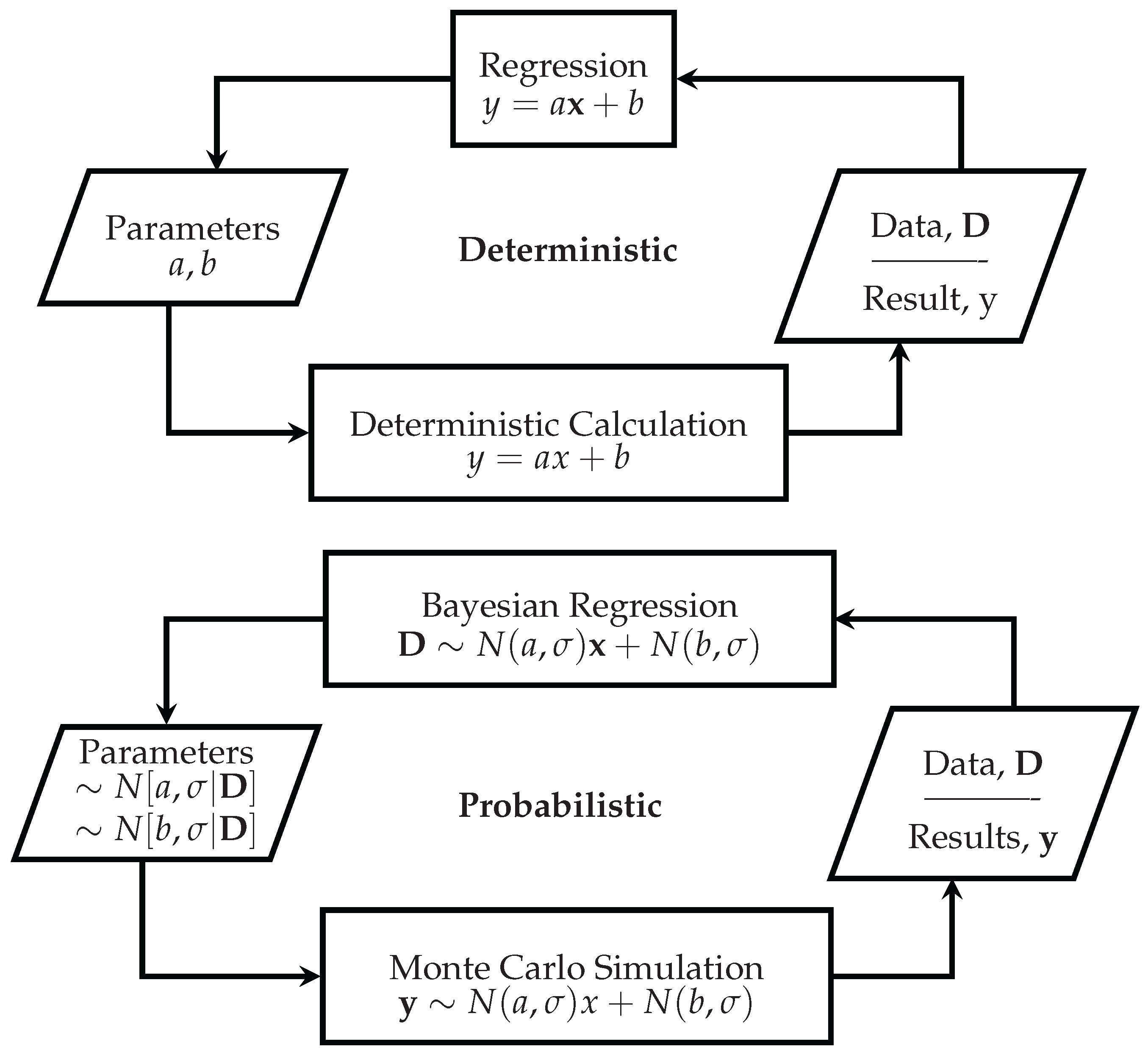
It is this inversion process that has often been intractable in higher dimensions until the advent of Markov Chain Monte Carlo (MCMC) techniques and increased computing power (Technical note: other Monte Carlo-based inversion techniques such as rejection or importance sampling are only efficient enough to be practical in low-dimensional settings. Note that we use Monte Carlo here in the sense of a straightforward sense of generating random numbers according to standard distributions [13]). MCMC software has allowed users to specify a model (e.g., a linear regression model), supply the observations or data (measurements), and infer the values on the model parameters probabilistically. This is called probabilistic programming. Probabilistic programming is compelling because, instead of working with point estimates on all unknown parameters (e.g., slope and intercept in a straight-line regression model), one describes the system in terms of probability distributions. Working with probability distributions rather than point estimates is preferable, since it is well known that doing calculations with point estimates can lead to erroneous conclusions [14]. When doing forward-calculations as illustrated in Figure 1, it is therefore desirable to use distributions on unknown variables and then apply a Monte Carlo simulation or Mellin Transform Moment Calculation method [15,16] to obtain a probability distribution on the result. MCMC allows one to do the inverse: inferring parameter distributions from given data and a model. Therefore, MCMC is to regression what Monte Carlo simulation is to deterministic computation. The adoption of the Bayesian paradigm therefore allows the analyst to move from deterministic to probabilistic M&V, as shown in Figure 1.
For the inversion described above to work, the term, called the prior, needs to be specified. Although the prior can be used to incorporate information into the model, which is not available through the data alone, it is, in essence, merely a mathematical device allowing inversion. The prior is often specified as “non-informative”—a flat probability distribution over the region of interest, allowing the data to “speak for itself” through the likelihood term. This will be discussed in more detail below. The other term, , need not be specified in numeric MCMC models—it is a normalising factor ensuring that the right-hand side of the equation can integrate to unity, making it a proper probability density function (Technical note: this term becomes important in more sophisticated Bayesian analyses where model selection or experimental design is done [1]). The left-hand side of the equation is called the posterior distribution and is proportional, therefore, to the product of the prior and the likelihood.
Advanced Bayesian models may be nuanced, but the fundamental mechanics as described above stay the same for all Bayesian analyses: specify priors, describe the likelihood, and solve to find the posterior on the parameters of interest.
2.1. Practical Benefits
Besides the theoretical attractiveness discussed above, the Bayesian paradigm also offers many practical benefits for energy M&V:
- Because Bayesian models are probabilistic, uncertainty is automatically and exactly quantified.
- Uncertainty calculations in the Bayesian approach can be much less conservative than standard approaches. Shonder and Im [17] show a 40% reduction in uncertainty in one case. Since project payment is often dependent on savings uncertainties being within certain bounds, using the Bayesian approach can increase project feasibility.
- By making the priors and energy model explicit, the Bayesian approach ensures greater transparency—one of the five key principles of M&V [5].
- The Bayesian approach is widely used and is rapidly gaining popularity in other scientific fields. Lira [18] relates that even the GUM (adopted by many societies of physics, chemistry, electrotechnics, etc.) is being rewritten to be more consistent with this approach. Since M&V reports uncertainty according to the GUM, Bayesian calculations would be useful.
- Bayesian models are more universal and flexible than standard methods. Bayesian modelling can be highly sophisticated, but the core of probabilistic thinking is consistent throughout. This is different to frequentist statistics where knowledge of one or even many tests will not necessarily aid the analyst in understanding a new metric, or approach to a problem not seen before. Many frequentist tests are ad hoc and apply only to specific situations. For example, t-tests have little to do with regression in frequentism, but, in Bayesian thinking, they are expressions of the same idea.
- Being modular, Bayesian modelling is more flexible. Ordinary least squares (OLS) linear regression assumes residuals are normally distributed and that the variance is constant for all points. In a probabilistic Bayesian model, the parameters can be distributed according to any distribution, but the posterior for each will be determined by the data (if the prior is appropriately chosen). Models are also modular and can be designed to suit the problem. For example, it is no different to create terms for serial correlation, or heteroscedasticity (non-constant variance) than it is to specify an ordinary linear model. This also allows for easy specification of non-routine adjustments, the handling of missing values, and the incorporation of unmeasured yet important quantities such as measurement error, often problematic for energy models. For the retrofit isolation with a key parameter measurement approach, the unmeasured parameters (the estimates) can also be incorporated in this way.
- Bayesian models can account for model-selection uncertainty. There are often multiple reasonable energy models which could describe a specific case—for example: time and dry-bulb temperature; occupancy and dry-bulb temperature; temperature, humidity, and occupancy, etc. The analyst usually chooses one model, discards the rest, and reports the uncertainty produced in that specific model. However, this uncertainty does not account for model selection. In other words, there is an uncertainty associated with choosing that specific model above another reasonable one. Bayesian model averaging allows many models to be specified simultaneously, and averages their results by automatically weighting each model’s influence on the final result by that model’s explanatory power. This gives a far more realistic uncertainty value [4].
- Because uncertainty is automatically quantified, CIs can be interpreted in the way most people understand them: degrees of belief about the value of the parameter.
- The Bayesian approach is well-suited to “small data” problems. This seems like a minor point in developed countries where questions surrounding big data are more pressing. However, big (energy) data is a decidedly “first-world problem”. In developing countries, a lack of meters makes M&V expensive, and it is useful to have a method that is consistent on smaller data sets as well.
- Bayesian approaches allow real-time or online updating of estimates [19,20,21]. For many other machine learning techniques, the data need to be split into testing and training sets, the model trained on the training set, and then used to predict the testing set period. As new data becomes available, the model needs to be retrained in many cases (Technical note: Artificial Neural Networks (ANNs), stochastic gradient descent and passive-aggressive algorithms, as well as Dynamic Linear Models can also be updated online), making it computationally expensive to keep a model updated. In a Bayesian paradigm, previous data can be summarised by the prior so that the model need not be retrained.
- The Bayesian approach allows for the incorporation of prior information where appropriate. The danger in this will be discussed in Section 2.2. However, in cases where it is warranted, known values or ranges for certain coefficients can be specified in the prior. This has been done successfully for energy projects [22,23,24,25]. Prior information is also useful in longitudinal studies, where measurements or samples from previous years can be taken into account [20,21].
- When the savings need to be calculated for “normalised conditions”, for example, a ‘typical meteorological year’, rather than the conditions during the post-retrofit monitoring period, it is not possible to quantify uncertainty using current methods. However, Shonder and Im [17] have shown that it can be naturally and easily quantified using the Bayesian approach.
2.2. Caveats
The Bayesian approach also comes with certain caveats that M&V practitioners and policy makers should bear in mind.
- Modelling is non-generic. In point 5 above, it was stated that the Bayesian approach is more universal. This is true in the sense that the same basic approach is used for many different kinds of problems. However, the inherent modularity of the method as described in point 6 means that there is not a one-size-fits-all generic template in Bayesian modelling, the way there usually is in frequentist modelling. This necessitates more thinking from the analyst. However, we believe this to be an advantage: frequentist approaches make it easier to think less, but as a consequence, also to build poor models, which has led to the current replication crisis seen in research [26] and a general mistrust of statistical results [27]. High quality models require some thought and care, in any paradigm.
- As with any method, it is not immune to abuse. The most popular criticism is that, by having a prior distribution on the savings, the posterior may be biased in a way not warranted by the data, making the result subjective. This is certainly possible. However, having a prior in an M&V analysis is actually an advantage.
- (a)
- As stated above, it allows for greater modelling transparency. The Bayesian form forces the analyst to be explicit about his or her modelling assumptions, and to defend them. Such assumptions cannot be imported by (accidentally or purposefully) choosing one test over another, as in the frequentist case.
- (b)
- It is sometimes necessary to include priors to avoid bias. Ioannidis [28] and Button [29] have shown that many medical studies contain false conclusions due to biased results. The bias that was introduced was to consider positive and negative outcomes from a clinical trial equally likely. However, the prior odds of an experimental treatment working is much lower than the odds of that treatment not working. Ignoring these prior odds leads to a high false-positive rate, since many of the positive results are actually false and due to noise. In M&V, the situation is reversed: the prior odds of energy projects saving energy are high. Having a neutral prior would therefore bias a result towards conservatism (Technical note: conservatism is one of the key principles of M&V [5], but we do not hereby advocate for neutral priors in all cases). Nevertheless, Button’s study is an excellent illustration of why priors are an important part of probability calculus.
- (c)
- Because the assumptions and distributions used are clearly stated, it precludes hedging the M&V result with phrases such as “however, from previous studies/experience, we know that this is a conservative figure ⋯”. Because the prior was stated and defended at the outset, the final result should already incorporate it and should not be hedged.
- (d)
- The thorough analyst will test the effect of different priors on the posterior, demonstrating the bias introduced through his modelling assumptions, and justifying its use.
- Bayesian methods can be computationally expensive for large datasets and complex models. It is true that numerical solvers are becoming more efficient and computational power is increasing. However, in comparison with matrix inversion techniques used for linear regression, for example, Bayesian methods are much slower and may be inappropriate for real-time applications [30].
- The forecasting accuracy of other machine learning (ML) methods can be higher than regression in some cases [31,32], although regression-based approaches such as time-of-week-and-temperature [33] still perform very well [32,34] and may be preferred for simplicity. Note that this is a limitation of regression, not the overall Bayesian paradigm, although regression is the way most M&V analysts would use Bayesian methods. Many ML techniques also have Bayesian approaches, for example Bayesian tree-based ensemble methods [35] or Bayesian Artificial Neural Networks [36,37]. It also depends on the problem: it is not possible to know beforehand which model will work the best [38]. ML algorithms without Bayesian implementations also still only produce point estimates. Therefore, they cannot be compared to the full probabilistic approach, which provides much richer information and is not just a forecasting technique, but a full inference paradigm.
- The parametric from of the model needs to be specified. Parametric Bayesian models as described in most of this study can only be correct in so far as their functional form describes the underlying physical process. Functional form misspecification is a real possibility. This is different to the machine learning methods described in the previous paragraph, which do not rely on a functional form being specified. Non-parametric models have their own benefits and limitations: for cases where the underlying physical process is well-understood, a parametric model can be more accurate. However, non-parametric methods such as Gaussian Processes (GPs) [22,39] or Gaussian Mixture Models [40] still require some model specification at a higher level (hyperparameters). GP models, for example, rely on an appropriate covariance function for valid inference. For more information on GPs for machine learning, see Rasmussen and Williams [41].
3. Bayesian M&V Examples
To demystify the Bayesian approach, two basic M&V calculations will be demonstrated. The reader will notice the recurring theme of expressing all variables as (conditional) probability distributions.
3.1. Sampling Estimation
Consider the following example from the IPMVP 2012 [5] (Appendix B-1). Twelve readings are taken by a meter. These are reported as monthly readings, but are assumed to be uncorrelated with any independent variables or other readings, and are therefore construed to be random samples. The values are:
The units are not reported and the results below are therefore left dimensionless, although kWh would be a reasonable assumption. These data were carefully chosen, and have a mean , sample standard deviation .
3.1.1. IPMVP Solution
The standard error is . The confidence interval on the mean is calculated as:
Since , the 90% confidence interval on the mean was calculated as , or a 7.7% precision. Metering uncertainty is not considered in this calculation.
3.1.2. Bayesian Solution
The Bayesian estimate of the mean is calculated as follows. First, prior distributions on the data need to be specified. Vague priors will be used:
A t-distribution will be used for the likelihood below, and the degrees of freedom parameter () of this distribution will, therefore, need to be specified. One could fix for the t-distribution at 12, since there are twelve data points and traditionally has been taken to signify this number. However, if outliers are present or if the data has more or less dispersion than the standard t-distribution with as many data points, this would not be realistic. It is therefore warranted to indicate the uncertainty in the data by specifying a prior distribution on also: a hyperprior. Kruschke [42] recommends an exponential distribution with the mean equal to the number of data points. This allows equal probability of being higher or lower than the default value:
If the vector of the parameters is , then the likelihood can be written as:
Note that the t-distribution is not used because of the t-test, but because its heavier tails are more accommodating of outliers. Any distribution could have been specified if there was good reason to do so. The posterior on is plotted in Figure 2. It was simulated in PyMC3 using the Automatic Differentiation Variational Inference (ADVI) algorithm with 100,000 draws, which is stable and converges on the posterior distribution in 10.76 s on a middle-range laptop computer. Although the mathematical notation may seem intimidating to practitioners who are not used to it, writing this in the probabilistic Python programming package PyMC3 [43] demonstrates the intuitive nature of such a model:
| import pymc3 as pm |
| with pm.Model() as bayesian_sampling_model: |
| # Hyperpriors and priors: |
| mean = pm.Uniform(’mean’, 0, 2000) |
| std = pm.Uniform(’std’, 0, 1000) |
| nu = pm.Exponential(’nu’, 1/len(data)) |
| # Likelihood |
| likelihood = pm.StudentT(’likelihood’, mu=mean, sd=std, nu=nu, observed=data) |
| # ADVI calculation |
| trace = pm.variational.sample_vp(vparams=pm.variational.advi(n=100000)) |
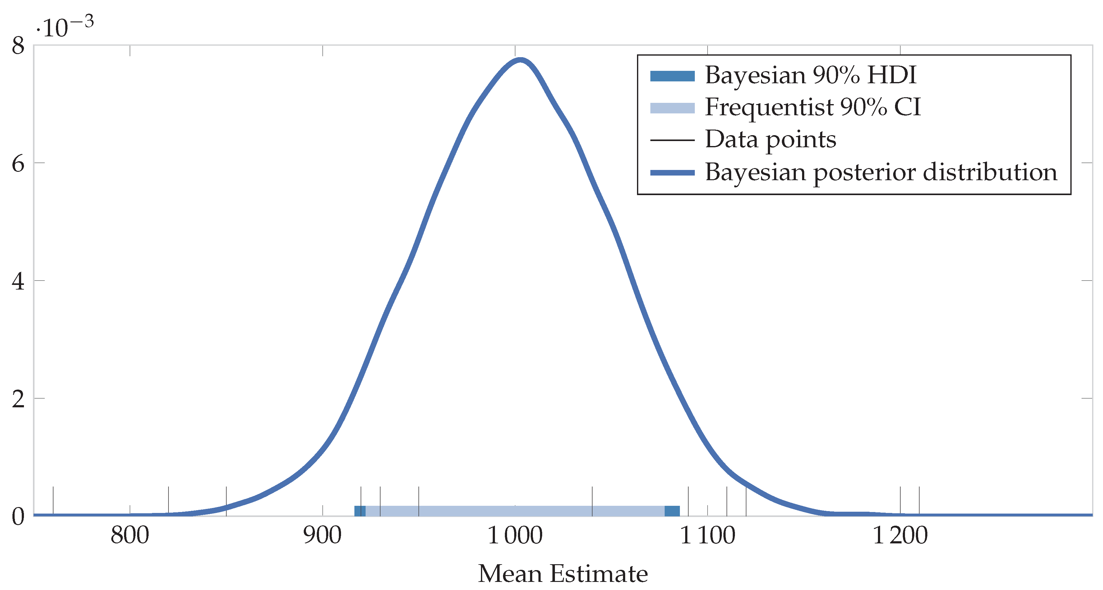
It is important to note that no probability statements about the values inside the frequentist interval can be made, nor can one fit a distribution to the interval. The distribution indicated is strictly a Bayesian one. The Bayesian (highest density) interval is slightly wider than the frequentist confidence interval, at a precision of 8.5%. If were fixed at 12 (indicating that we are certain that the data does indeed reflect a t-distribution with 12 degrees of freedom exactly), Bayesian and frequentist intervals correspond exactly. However, the Bayesian alternative allows for a more realistic value. With comparisons between two groups (two-sample t-tests), the effect of uncertainty in the priors becomes even more pronounced [42].
The posterior distribution can now be used to answer many interesting questions. For instance, what is the probability, given the data at hand, that the true mean is below 900? Or, is it safe to assume that the standard value of 950 is reflected by this sample, or should the null hypothesis be rejected? (If previous data to this effect is available, it could be included in the prior, maybe using the equivalent prior sample size method [44]). The frequentist may say that there is not enough evidence to reject the null, but cannot accept it either. In the Bayesian paradigm, 950 falls comfortably within the 90% confidence range, and can therefore be accepted at that level. As a further question, if this is an energy performance contracting project, and we assume that the data points are different facilities rather than different months, would it be worthwhile taking a larger sample to increase profits, if we believe that the true mean is 1100 (on which see Lindley [45], Bernardo [46] and Goldberg [47]).
It is therefore evident that the Bayesian result yields richer and more useful information using intuitive mathematics.
3.2. Regression
In M&V, one often uses the baseline data () to infer the baseline (pre-retrofit) model parameters through an inverse method:
where is a function relating the independent variables (energy governing factors) to the energy use of the facility, and is time. The model parameters describe the sensitivity of the energy model to the independent variables such as occupancy, outside air temperature, or production volume.
As an aside, this section will discuss an elementary parametric energy model using Bayesian regression, similar to standard linear regression. In practice, a two-parameter linear regression model seldom captures the different states of a facility’s energy use, for example, heating at low temperatures, a comfortable range, and cooling at high temperatures. Piecewise linear regression techniques are often used [48,49,50,51,52], and they tend to work reasonably well if their assumptions are satisfied, but they are not stable in all cases, are approximate, and the assumptions are often restrictive. Shonder and Im [17] provide a Bayesian alternative. A non-parametric model using a Gaussian Process could also be used, and since one does not need to specify a parametric model, it allows very flexible models to be fit while still quantifying uncertainty. This is especially useful for models where energy use is a nonlinear function of the energy governing factors. However, to keep the example simple and focussed, only a simple parametric model will be considered below.
3.2.1. Example
Suppose one has a simple regression model where the energy use of a building is correlated with the outside air temperature through the number of Cooling Degree Days (CDD). One cooling degree day is defined as an instance where the average daily temperature is one degree above the thermostat set point for one day, and the building therefore requires one degree of cooling (Technical note: a more accurate description would be the “building balance point”, where the building’s mass and insulation balance external forcings [53]). Let the intercept coefficient be , the slope coefficient , and the Gaussian error term . One could then write:
In standard linear regression, one would write as the vector of two coefficients and do some linear algebra to obtain their estimates. There would be a standard error on each, which would indicate their uncertainties, and if the assumptions of linear regression, such as normality of residuals, independence of data, homoscedasticity, etc. hold, then it would be accurate. In Bayesian regression, one would describe the distributions on the parameters:
where is the vector of the standard deviations on the estimates. Generating random pairs of values from the posterior, at a given value of CDD, according to the appropriate distributions, will yield the posterior predictive distribution. This is the distribution of energy use at a given temperature, or over the range of temperatures. Overlaying such realisations onto the actual data is called the posterior predictive check (PPC).
Now, consider a concrete example. The IPMVP 2012 [5] (Appendix B-6) contains a simple regression example of creating a baseline of a building’s cooling load. The twelve data points themselves were not given, but a very similar data set yielding almost identical regression characteristics has been engineered and is shown in Table 1.
A linear regression model was fit to the data, and yielded the result shown in Table 2.
3.2.2. IPMVP Solution
The IPMVP then proceeds to calculate the uncertainty in the annual energy figure by multiplying the standard error on the estimate (the average standard error) by and the average consumption in the average month, and assumes that this value is constant for all months. As discussed in this study, this approach is problematic, and can at best be seen as approximate. Since it is treated in some detail in the IPMVP, the analysis will not be repeated here.
3.2.3. Bayesian Solution
The key to the Bayesian method is to approach the problem probabilistically, and therefore view all parameters in Equation (9) as probability distributions, and specify them as such. In this regression model, there are three parameters of interest: the intercept (), slope (), and the response (). This response is the likelihood function, familiar to most readers as the frequentist approach. These distributions need to be specified in the Bayesian model. First, consider the priors on the slope and intercept. These can be vague. Technical note: the uniform prior on in Equation (11) is actually technically incorrect: it may seem uniform in terms of gradient but is not uniform when the angle of the slope is considered. It is therefore not “rotationally invariant” and biases the estimate towards higher angles [54]. The correct prior is ; this is uniform on the slope angle. The reason that Equation (11) works in this case is that the exponential weight of the likelihood masks the effect. However, this is not always the case, and analysts should be careful of such priors in regression analysis:
and
Now, consider the likelihood. In frequentist statistics, one needs to assume that in Equation (9) is normally distributed. In the Bayesian paradigm, one may do so, but it is not necessary. A Student’s t-distribution is often used instead of a Normal distribution in other statistical calculations (e.g., t-tests) due to its additional (“degrees of freedom”) parameter, which accommodates the variance arising from small sample sizes more successfully. As in Section 3.1.2, an exponential distribution on the degrees of freedom () is specified. It has also been found that specifying a Half-Cauchy distribution on the standard deviation () works well [55]. Therefore, the hyperpriors are specified as:
and:
The mean of the likelihood is the final hyperparameter that needs to be specified. This is simply Equation (9), written with the priors:
The full likelihood can thus be written as:
The PyMC3 code is shown below:
| import pymc3 as pm |
| with pm.Model() as bayesian_regression_model: |
| # Hyperpriors and priors: |
| nu = pm.Exponential(’nu’, lam=1/len(CDD)) |
| sigma = pm.HalfCauchy(’sigma’, beta=1) |
| slope = pm.Uniform(’slope’, lower=0, upper=20) |
| intercept = pm.Uniform(’intercept’, lower=0, upper=10000) |
| # Energy model: |
| regression_eq = intercept + slope*CDD |
| # Likelihood: |
| y = pm.StudentT(’y’, mu=regression_eq, nu=nu, sd=sigma, observed=E) |
| # MCMC calculation: |
| trace = pm.sample(draws=10000, step=pm.NUTS(), njobs=4) |
The last line of the code above invokes the MCMC sampler algorithm to solve the model. In this case, the No U-Turn Sampler (NUTS) [56] was used, running four traces of 10,000 samples each, simultaneously on a four-core laptop computer, in 3.5 min fewer samples, could also have been used.
A discussion of the inner workings and tests for adequate convergence of the MCMC is beyond the scope of the study and has been done in detail elsewhere in literature [4]. The key idea for M&V practitioners is that the MCMC, like MC simulation, must converge, and must have done enough iterations after convergence to approximate the posterior distribution numerically. For most simple models such as the ones used in most M&V applications, a few thousand iterations are usually adequate for inference. Two popular checks for posterior validity are the Gelman–Rubin statistic [57,58] and the effective sample size (ESS). The Gelman–Rubin statistic compares the four chains specified in the program above, started at random places, to see if they all converged on the same posterior values. If they did, their ratios should be close to unity. This is easily done in PyMC3 with the pm.gelman_rubin(trace) command, which indicates equal to one to beyond the third decimal place. However, even if the MCMC has converged, it does not mean that the chain is long enough to approximate the posterior distribution adequately because the MCMC mechanism produces a serially correlated (autocorrelated) chain. It is therefore necessary to calculate the effective sample size: the sample size taking autocorrelation into account. In PyMC3, one can invoke the pm.effective_n(trace) command, which shows that the ESSs for the parameters of interest are well over 1000 each for the current case study. As a first-order approximation, we can therefore be satisfied that the MCMC has yielded satisfactory estimates.
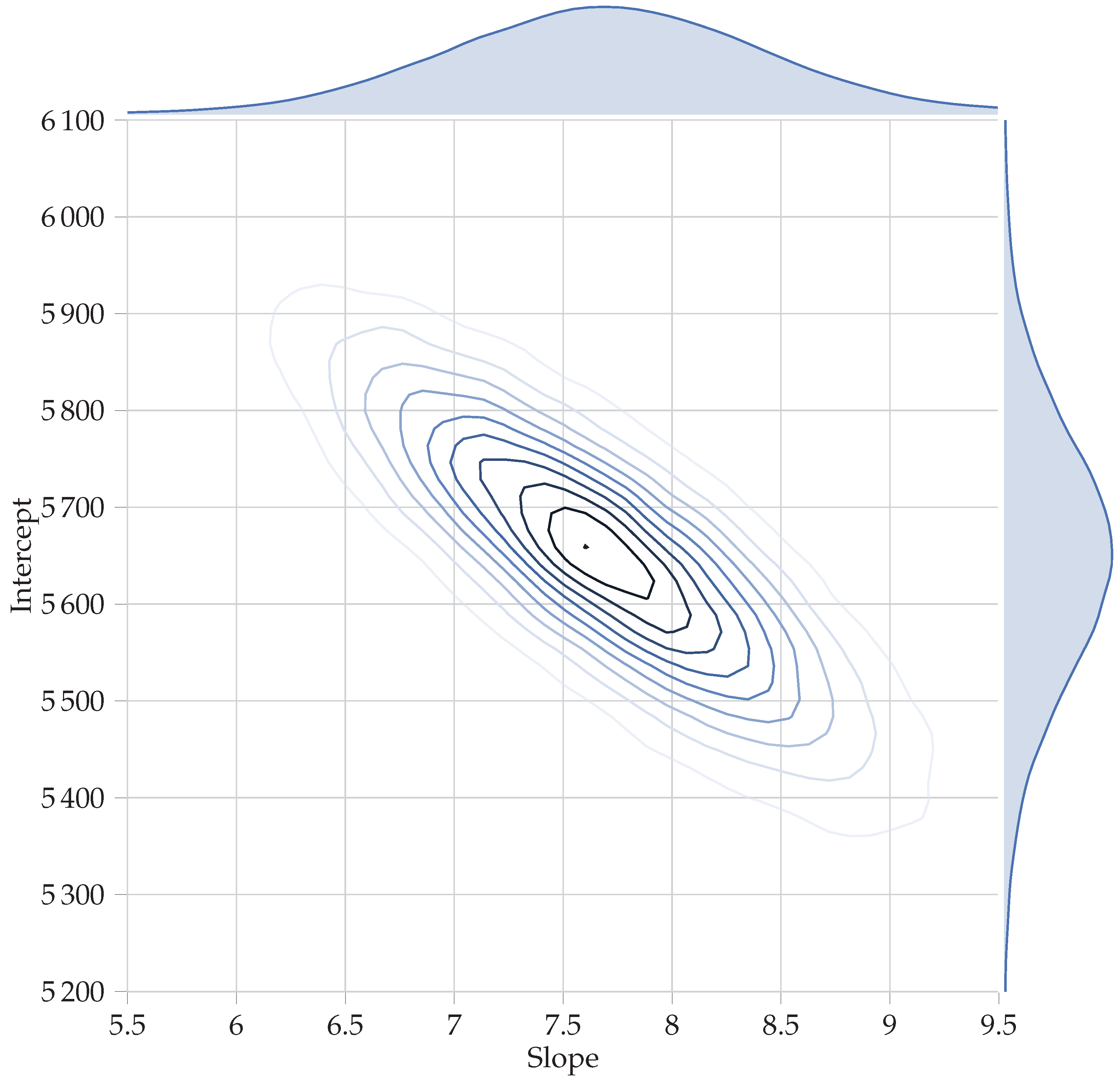
The MCMC results can be inspected in various ways. The posteriors on the parameters of interest are shown in Figure 3. If a normal distribution is specified on the likelihood in Equation (16) rather than the Student’s t, the posterior means are identical to the linear regression point estimates—an expected result, since OLS regression is a special case of the more general Bayesian approach. Using a t-distributed likelihood yields slightly different, but practically equivalent, results. The mean or mode of a given posterior is not of as much interest as the full distribution, since this full distribution will be used for any subsequent calculation. However, the mean of the posterior distribution(s) is given in Table 3 for the curious reader.
Two brief notes on Bayesian intervals are necessary. As discussed in Section 1.1, the frequentist ‘confidence’ interval is a misnomer. To distinguish Bayesian from frequentist intervals, Bayesian intervals are often called ‘credible’ intervals, although they are much closer to what most people think of when referring to a frequentist confidence interval. The second note is that Bayesians often use HDIs, also known as highest posterior density intervals. These are related to the area under the probability density curve, rather than points on the x-axis. In frequentist statistics, we are used to equal-tailed confidence intervals since we compute them by taking the mean, and then adding or subtracting a fixed number—the standard error multiplied by the t-value, for example. This works well for symmetrical distributions such as the Normal, as is assumed in many frequentist methods. However, real data distributions are often asymmetrical, and forcing an equal-tailed confidence interval onto an asymmetric distribution leads to including an unlikely range of values on the one side, while excluding more likely values on the other. An HDI solves this problem. It does not have equal tails but has equally-likely upper and lower bounds.
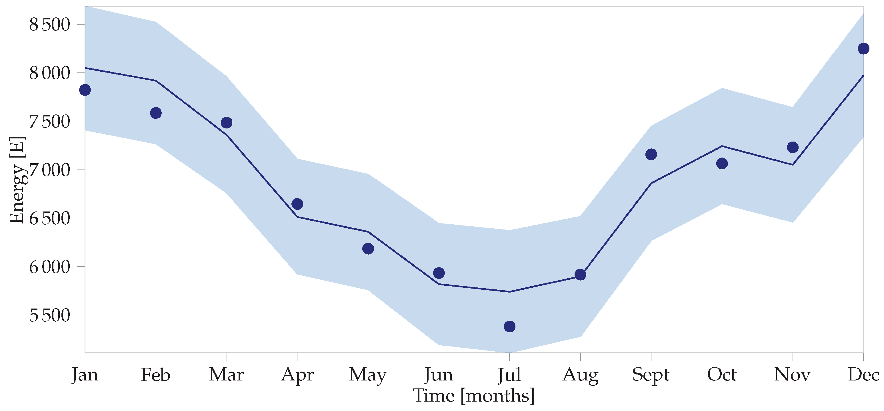
The posterior distributions shown in Figure 3 are seldom of use in themselves and are more interesting when combined in a calculation to determine the uncertainties in the baseline as shown in Figure 4, also known as the adjusted baseline. To do so, the posterior predictive distribution needs to be calculated using the pm.sample_ppc() command, which resamples from the posterior distributions, much like the MC simulation forward-step of Figure 1.
The Bayesian model can also be used to calculate the adjusted baseline, or what the post-implementation period energy use would have been, had no intervention been made. The difference between this value and the actual energy use during the reporting period is the energy saved. For the example under consideration, the IPMVP assumes that an average month in the post-implementation period: one with 162 CDDs. It also assumes that the actual reporting period energy use is 4300 kWh, measured with negligible metering error.
To calculate the savings distribution using the Bayesian method, one would do an MC simulation of:
where and are the distributions shown in Figure 3. Note that they are correlated and so using the PPC method described above would be the correct approach. Running this simulation with 10,000 samples yields the distribution shown in Figure 5. The 95% HDI is [2229, 2959], while the frequentist interval is [1810, 3430] for the same data—a much wider interval. Furthermore, the IPMVP then assumes averages and multiplies these figures to get annual savings and uncertainties. In the Bayesian paradigm, the HDIs can be different for every month (or time step) as shown in Figure 4, yielding more accurate overall savings uncertainty values.
3.2.4. Robustness to Outliers
As alluded to above, using the Student’s t-distribution rather than the normal distribution allows for Bayesian regression to be robust to outliers [59]. The heavier tails more easily accommodate an outlying data point by automatically altering the degrees-of-freedom hyperparameter to adapt to the non-normally distributed data. Uncertainty in the estimates is increased, but this reflects the true state of knowledge about the system more realistically than alternative assumptions of light tails, and is therefore warranted. The robustness of such regression does not give the M&V practitioner carte blanche to ignore outliers. One should always seek to understand the reason for an outlier; if the operating conditions of the facility were significantly different, the analyst should consider neglecting (or ‘condoning’) the data point. However, it is not always possible to trace the reasons for all outliers, and inherently robust models are useful (Technical note: the treatment here is very basic, and for illustration. More advanced Bayesian approaches are also available. For example, if there are only a few outliers, a mixture model may be used [60]. If there is a systematic problem such an unknown error variable, one can “marginalise” the offending variable out. The right-hand and top distributions of Figure 3 are marginal distributions: e.g., the distribution on the slope, with the intercept marginalised out, and vice versa. For an M&V example of marginalisation where an unknown measurement error is marginalised out, see Carstens [61] (Section 3.5.3). von der Linden et al. provides a thorough treatment of all the options for dealing with outliers [3] (Ch. 22)).
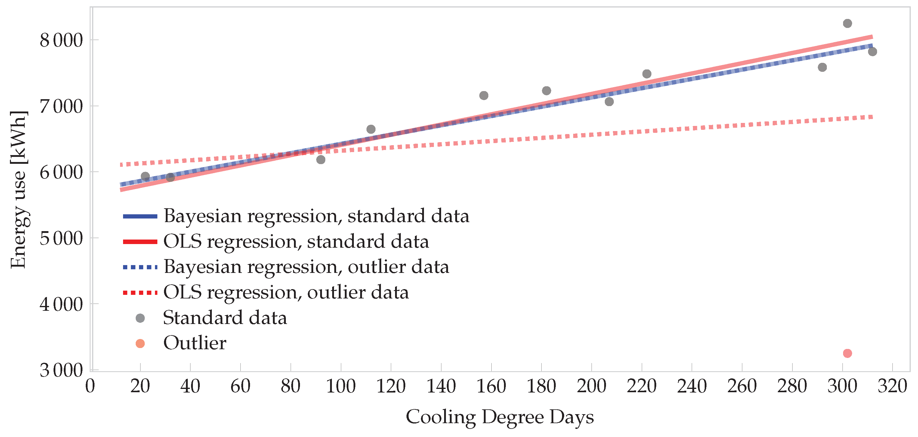
To demonstrate the robustness of such a Bayesian model, consider the regression case above. Suppose that for some reason the December cooling load was 3250 kWh and not 8250 kWh, indicated by the red point in the lower right-hand corner of Figure 6. If OLS regression were used, and this point is not removed, it would skew the whole model. However, the t-distributed likelihood in the Bayesian model is robust to the outlier. The effect is demonstrated in Figure 6. Four lines are plotted: the solid lines are for the data set without the outlier. The dashed lines are for the data set with the outlier. In the Bayesian model, the two regression lines are almost identical and close to the OLS regression line for the standard set. However, the OLS regression on the outlier set is dramatically biased and would underestimate the energy use for hot months due to the outlier.
3.2.5. Hierarchical Models
A further advantage in the Bayesian paradigm is the use of hierarchical, or multilevel models. This is a feature of the model structure rather than the Bayesian calculation itself (it also works for MLE) [2], but it is nevertheless useful in M&V. Suppose that multiple measures are installed at multiple sites so that the IPMVP Option C: Whole Building Retrofit is used for M&V. The UMP Chapter 8 [62] reports that there are two ways to analyse such data. The two-stage approach involves first analysing each facility separately and then using these results for the overall analysis in stage two. The fixed effects approach analyses all buildings simultaneously but assumes that the effect sizes are constant across facilities, using an average effect for all buildings. Hierarchical modelling considers both the individual facility’s energy saving and the overall effect simultaneously. It does this by assuming that the group effects are different realisations of an overarching distribution with a mean and variance, which is used as a prior. This can lead to ‘shrinkage’ in the parameter uncertainty estimates because the group effects are mutually informative. For groups with little data, the overarching effect distribution plays a larger role, and for groups with more data, a smaller role. In addition, the overall variance is reduced because the sources of inter-facility variance are isolated from that of inter-measure variance. The result for a hierarchical model is that the effect estimation for an individual facility is influenced by the overall estimate of the measured effect, as well as by the data for the facility. As another example, consider a program that retrofits air conditioning units in different provinces in South Africa. One could fix the savings effect across all facilities, but this will underestimate some and overestimate others. Otherwise, one could analyse by facility, then by province, and then overall. The hierarchical model provides a better alternative in these cases, and comprises the bulk of many Bayesian data analysis texts [2,4]. Booth, Choudhary, and Spiegelhalter have provided an excellent example of using hierarchical Bayesian models in energy M&V [63].
4. Bayesian Alternatives for Standard M&V Analyses
At this point, an M&V analyst may want to try the Bayesian method for an M&V problem, but where to start? In Table 4, some Bayesian alternatives to standard M&V analyses are given. The references cited are mostly from M&V studies, although some general statistical sources are also listed where applicable.
5. Conclusions
The Bayesian paradigm provides a coherent and intuitive approach to energy measurement and verification. It does so by defining the basic M&V question—the savings inference given measurements—using conditional probabilities. It also provides a simpler and more intuitive understanding of probability and uncertainty because it allows the analyst to answer real questions in a straightforward manner, unlike traditional statistics. Due to recent technological and mathematical advances being incorporated into software, analysts need not be expert statisticians to harness the power and flexibility of this method.
The probabilistic nature of Bayesian analysis allows for automatic and accurate uncertainty quantification in savings models. The richer nature of the Bayesian result is shown in a sampling and a regression problem, where it is found that the Bayesian method allows for more realistic modelling and a greater variety of questions that can be answered. Its flexibility is also demonstrated by constructing a robust regression model, which is much less sensitive to outliers that standard ordinary least squares regression traditionally used in M&V.
Acknowledgments
The authors would like to thank Mark Rawlins, Pieter de Villiers, and Franco Barnard for their inputs to the draft of this study, as well as the anonymous reviewers whose detailed feedback improved the paper substantially.
Author Contributions
Herman Carstens conceived of and wrote this paper. Xiaohua Xia and Sarma Yadavalli led the study and his doctoral work in which some of these ideas were developed.
Conflicts of Interest
The authors declare no conflict of interest.
Abbreviations
The following abbreviations are used in this manuscript:
| ADVI | Automatic Differentiation Variational Inference |
| ANN | Artificial Neural Network |
| ASHRAE | American Society of Heating, Refrigeration, and Air Conditioning Engineers |
| CDD | Cooling Degree Days |
| CI | Confidence Interval |
| ESS | Effective Sample Size |
| GP | Gaussian Process |
| HDI | Highest Density Interval |
| IPMVP | International Performance Measurement and Verification Protocol |
| ISO | International Standards Organization |
| MC | Monte Carlo |
| MCMC | Markov Chain Monte Carlo |
| M&V | Measurement and Verification |
| PPC | Posterior Predictive Check |
| OLS | Ordinary Least Squares |
| UMP | Uniform Methods Project |
References
- Sivia, D.; Skilling, J. Data Analysis: A Bayesian Tutorial; Oxford University Press: Oxford, UK, 2006. [Google Scholar]
- Kruschke, J. Doing Bayesian Data Analysis: A Tutorial with R, JAGS, and Stan, 2th ed.; Academic Press: Cambridge, MA, USA, 2015. [Google Scholar]
- Von der Linden, W.; Dose, V.; Von Toussaint, U. Bayesian Probability Theory: Applications in the Physical Sciences; Cambridge University Press: Cambridge, UK, 2014. [Google Scholar]
- Gelman, A.; Carlin, J.B.; Stern, H.S.; Rubin, D.B. Bayesian Data Analysis; Taylor & Francis: Abingdon-on-Thames, UK, 2014; Volume 2. [Google Scholar]
- Efficiency Valuation Organization. International Performance Measurement and Verification Protocol; Efficiency Valuation Organization: Toronto, ON, Canada, 2012; Volume 1. [Google Scholar]
- International Organization for Standardization (ISO). Guide 98–3 (2008) Uncertainty of Measurement Part 3: Guide to the Expression of Uncertainty in Measurement (GUM: 1995); ISO: Geneva, Switzerland, 2008. [Google Scholar]
- American Society of Heating, Refrigeration and Air-Conditioning Engineers, Inc. Guideline 14-2014, Measurement of Energy, Demand, and Water Savings. 2014. Available online: https://ihsmarkit.com/products/ashrae-standards.html (accessed on 1 December 2017).
- National Renewable Energy Laboratory. Uniform Methods Project. Available online: https://energy.gov/eere/about-us/ump-home (accessed on 1 December 2017).
- Robert, C. The Bayesian Choice: From Decision-Theoretic Foundations to Computational Implementation; Springer Science & Business Media: Berlin/Heidelberg, Germany, 2007. [Google Scholar]
- Neyman, J. Outline of a theory of statistical estimation based on the classical theory of probability. Philos. Trans. R. Soc. Lond. Ser. A Math. Phys. Sci. 1937, 236, 333–380. [Google Scholar] [CrossRef]
- Montgomery, D.C.; Runger, G.C. Applied Statistics and Probability for Engineers; John Wiley & Sons: Hoboken, NJ, USA, 2010. [Google Scholar]
- Wasserstein, R.L.; Lazar, N.A. The ASA’s statement on p-values: Context, process, and purpose. Am. Stat. 2016, 70, 129–133. [Google Scholar] [CrossRef]
- Joint Committee for Guides in Metrology. OIML G1-101 Evaluation of Measurement Data—Supplement 1 to the “Guide to the Expression of Uncertainty in Measurement"—Propagation of Distributions Using a Monte Carlo Method; International Organization of Legal Metrology: Paris, France, 2008. [Google Scholar]
- Savage, S.L.; Markowitz, H.M. The flaw of Averages: Why We Underestimate Risk in the Face of Uncertainty; John Wiley & Sons: Hoboken, NJ, USA, 2009. [Google Scholar]
- Kuang, Y.C.; Rajan, A.; Ooi, M.P.L.; Ong, T.C. Standard uncertainty evaluation of multivariate polynomial. Measurement 2014, 58, 483–494. [Google Scholar] [CrossRef]
- Rajan, A.; Ooi, M.P.L.; Kuang, Y.C.; Demidenko, S.N. Analytical Standard Uncertainty Evaluation Using Mellin Transform. IEEE Access 2015, 3, 209–222. [Google Scholar] [CrossRef]
- Shonder, J.A.; Im, P. Bayesian Analysis of Savings from Retrofit Projects. ASHRAE Trans. 2012, 118, 367. [Google Scholar]
- Lira, I. The GUM revision: The Bayesian view toward the expression of measurement uncertainty. Eur. J. Phys. 2016, 37, 025803. [Google Scholar] [CrossRef]
- Tehrani, N.H.; Khan, U.T.; Crawford, C. Baseline load forecasting using a Bayesian approach. In Proceedings of the 2016 IEEE Canadian Conference on Electrical and Computer Engineering (CCECE), Vancouver, BC, Canada, 15–18 May 2016; pp. 1–4. [Google Scholar]
- Carstens, H.; Xia, X.; Yadavalli, S. Efficient Longitudinal Population Survival Survey Sampling for the Measurement and Verification of Building Retrofit Projects. Energy Build. 2017, 150, 163–176. [Google Scholar] [CrossRef]
- Carstens, H.; Xia, X.; Yadavalli, S. Efficient metering and surveying sampling designs in longitudinal Measurement and Verification for lighting retrofit. Energy Build. 2017, 154, 430–447. [Google Scholar] [CrossRef]
- Heo, Y. Bayesian Calibration of Building Energy Models for Energy Retrofit Decision-Making under Uncertainty. Ph.D. Thesis, Georgia Institute of Technology, Atlanta, GA, USA, 2011. [Google Scholar]
- Lee, B.D.; Sun, Y.; Augenbroe, G.; Paredis, C.J. Toward Better Prediction of Building Performance: A Workbench to Analyze Uncertainty in Building Simulation. In Proceedings of the 13th Conference of the International Building Performance Simulation Association (BS2013), Le Bourget Du Lac, France, 25–30 August 2013. [Google Scholar]
- Booth, A.; Choudhary, R. Decision making under uncertainty in the retrofit analysis of the UK housing stock: Implications for the Green Deal. Energy Build. 2013, 64, 292–308. [Google Scholar] [CrossRef]
- Heo, Y.; Graziano, D.J.; Guzowski, L.; Muehleisen, R.T. Evaluation of calibration efficacy under different levels of uncertainty. J. Build. Perform. Simul. 2015, 8, 135–144. [Google Scholar] [CrossRef]
- McShane, B.B.; Gal, D.; Gelman, A.; Robert, C.; Tackett, J.L. Abandon statistical significance. arXiv, 2017; arXiv:1709.07588. [Google Scholar]
- Leek, J.; Colquhoun, D.; McShane, B.B.; Gelman, A.; Nuijten, M.B.; Goodman, S.N. Comment: Five Ways to Fix Statistics. Nature 2017, 551, 557–559. [Google Scholar] [PubMed]
- Ioannidis, J.P. Why most published research findings are false. PLoS Med. 2005, 2, e124. [Google Scholar] [CrossRef] [PubMed] [Green Version]
- Button, K.S.; Ioannidis, J.P.; Mokrysz, C.; Nosek, B.A.; Flint, J.; Robinson, E.S.; Munafò, M.R. Power failure: Why small sample size undermines the reliability of neuroscience. Nat. Rev. Neurosci. 2013, 14, 365–376. [Google Scholar] [CrossRef] [PubMed]
- Pavlak, G.S.; Florita, A.R.; Henze, G.P.; Rajagopalan, B. Comparison of Traditional and Bayesian Calibration Techniques for Gray-Box Modeling. J. Archit. Eng. 2013, 20, 04013011. [Google Scholar] [CrossRef]
- Yildiz, B.; Bilbao, J.; Dore, J.; Sproul, A. Recent advances in the analysis of residential electricity consumption and applications of smart meter data. Appl. Energy 2017, 208, 402–427. [Google Scholar] [CrossRef]
- Gallagher, C.V.; Bruton, K.; Leahy, K.; O’Sullivan, D.T. The Suitability of Machine Learning to Minimise Uncertainty in the Measurement and Verification of Energy Savings. Energy Build. 2018, 158, 647–655. [Google Scholar] [CrossRef]
- Mathieu, J.L.; Price, P.N.; Sila, K.; Piette, M.A. Quantifying changes in building electricity use, with application to demand response. IEEE Trans. Smart Grid 2009, 41, 374–381. [Google Scholar] [CrossRef]
- Granderson, J.; Touzani, S.; Custodio, C.; Sohn, M.D.; Jump, D.; Fernandes, S. Accuracy of automated measurement and verification (M&V) techniques for energy savings in commercial buildings. Appl. Energy 2016, 173, 296–308. [Google Scholar]
- Chipman, H.A.; George, E.I.; McCulloch, R.E. BART: Bayesian additive regression trees. Ann. Appl. Stat. 2010, 4, 266–298. [Google Scholar] [CrossRef]
- Tran, D.; Kucukelbir, A.; Dieng, A.B.; Rudolph, M.; Liang, D.; Blei, D.M. Edward: A library for probabilistic modeling, inference, and criticism. arXiv, 2016; arXiv:1610.09787. [Google Scholar]
- Neal, R.M. Bayesian Learning for Neural Networks; Springer Science & Business Media: Berlin/Heidelberg, Germany, 2012; Volume 118. [Google Scholar]
- Wolpert, D.H. The Lack of A Priori Distinctions Between Learning Algorithms. Neural Comput. 1996, 8, 1341–1390. [Google Scholar] [CrossRef]
- Heo, Y.; Zavala, V.M. Gaussian process modeling for measurement and verification of building energy savings. Energy Build. 2012, 53, 7–18. [Google Scholar] [CrossRef]
- Zhang, Y.; O’Neill, Z.; Dong, B.; Augenbroe, G. Comparisons of inverse modeling approaches for predicting building energy performance. Build. Environ. 2015, 86, 177–190. [Google Scholar] [CrossRef]
- Rasmussen, C.E.; Williams, C.K. Gaussian Processes for Machine Learning; MIT Press: Cambridge, MA, USA, 2006; Volume 1. [Google Scholar]
- Kruschke, J.K. Bayesian Estimation Supersedes the t-Test. J. Exp. Psychol. Gen. 2013, 142, 573–603. [Google Scholar] [CrossRef] [PubMed]
- Salvatier, J.; Wiecki, T.V.; Fonnesbeck, C. Probabilistic programming in Python using PyMC3. PeerJ Comput. Sci. 2016, 2, e55. [Google Scholar] [CrossRef]
- Winkler, R.L. The assessment of prior distributions in Bayesian analysis. J. Am. Stat. Assoc. 1967, 62, 776–800. [Google Scholar] [CrossRef]
- Lindley, D.V. The choice of sample size. J. R. Stat. Soc. Ser. D (Stat.) 1997, 46, 129–138. [Google Scholar] [CrossRef]
- Bernardo, J. Statistical inference as a decision problem: The choice of sample size. J. R. Stat. Soc. Ser. D (Stat.) 1997, 46, 151–153. [Google Scholar] [CrossRef]
- Goldberg, M.L. Reasonable Doubts: Monitoring and Verification for Performance Contracting. In Proceedings of the 1996 ACEEE Summer Study on Energy Efficiency in Buildings, Pacific Grove, CA, USA, 25–31 August 1996; Volume 4, pp. 133–143. [Google Scholar]
- Ruch, D.; Kissock, J.; Reddy, T. Prediction uncertainty of linear building energy use models with autocorrelated residuals. J. Sol. Energy Eng. 1999, 121, 63–68. [Google Scholar] [CrossRef]
- Kissock, J.K.; Haberl, J.S.; Claridge, D.E. Inverse modeling toolkit: Numerical algorithms (RP-1050). Trans.-Am. Soc. Heat. Refrig. Air Cond. Eng. 2003, 109, 425–434. [Google Scholar]
- Reddy, T.; Claridge, D. Uncertainty of “measured” energy savings from statistical baseline models. HVAC&R Res. 2000, 6, 3–20. [Google Scholar]
- Walter, T.; Price, P.N.; Sohn, M.D. Uncertainty estimation improves energy measurement and verification procedures. Appl. Energy 2014, 130, 230–236. [Google Scholar] [CrossRef]
- Mathieu, J.L.; Callaway, D.S.; Kiliccote, S. Variability in automated responses of commercial buildings and industrial facilities to dynamic electricity prices. Energy Build. 2011, 43, 3322–3330. [Google Scholar] [CrossRef]
- Berk, H.; Ascazubi, M.; Bobker, M. Inverse Modeling of Portfolio Energy Data for Effective Use with Energy Managers; Building Simulation: San Francisco, AR, USA, 2017. [Google Scholar]
- VanderPlas, J. Frequentism and Bayesianism: a Python-driven primer. arXiv, 2014; arXiv:1411.5018. [Google Scholar]
- Gelman, A. Prior distributions for variance parameters in hierarchical models (comment on article by Browne and Draper). Bayesian Anal. 2006, 1, 515–534. [Google Scholar] [CrossRef]
- Hoffman, M.D.; Gelman, A. The no-U-turn sampler: Adaptively setting path lengths in Hamiltonian Monte Carlo. J. Mach. Learn. Res. 2014, 15, 1593–1623. [Google Scholar]
- Gelman, A.; Rubin, D.B. Inference from iterative simulation using multiple sequences. Stat. Sci. 1992, 457–472. [Google Scholar] [CrossRef]
- Brooks, S.P.; Gelman, A. General methods for monitoring convergence of iterative simulations. J. Comput. Graph. Stat. 1998, 7, 434–455. [Google Scholar]
- Lange, K.L.; Little, R.J.; Taylor, J.M. Robust statistical modeling using the t distribution. J. Am. Stat. Assoc. 1989, 84, 881–896. [Google Scholar] [CrossRef]
- Press, W.H. Understanding data better with Bayesian and global statistical methods. arXiv, 1996; arXiv:astro-ph/9604126. [Google Scholar]
- Carstens, H. A Bayesian Approach to Energy Monitoring Optimization. Ph.D. Thesis, University of Pretoria, Pretoria, South Africa, 2017. [Google Scholar]
- Agnew, K.; Goldberg, M. The Uniform Methods Project: Methods for Determining Energy Efficiency Savings for Specific Measures; Whole-Building Retrofit with Consumption Data Analysis Evaluation Protocol; National Renewable Energy Laboratory: Golden, CO, USA, 2013; Chapter 8. [Google Scholar]
- Booth, A.; Choudhary, R.; Spiegelhalter, D. A hierarchical Bayesian framework for calibrating micro-level models with macro-level data. J. Build. Perform. Simul. 2013, 6, 293–318. [Google Scholar] [CrossRef]
- Gelman, A. Analysis of variance—Why it is more important than ever. Ann. Stat. 2005, 33, 1–53. [Google Scholar] [CrossRef]
- Burkhart, M.C.; Heo, Y.; Zavala, V.M. Measurement and verification of building systems under uncertain data: A Gaussian process modeling approach. Energy Build. 2014, 75, 189–198. [Google Scholar] [CrossRef]
- Carstens, H.; Rawlins, M.; Xia, X. A user’s guide to the SANAS STC WG guideline for reporting uncertainty in measurement and verification. In Proceedings of the South African Energy Efficiency Confederation Conference, Kempton Park, South Africa, 14–15 November 2017. [Google Scholar]
- Carstens, H.; Xia, X.; Yadavalli, S. Low-cost energy meter calibration method for measurement and verification. Appl. Energy 2017, 188, 563–575. [Google Scholar] [CrossRef]
Figure 1.
Deterministic and probabilistic calculation, simulation, and inverse modelling. The notation denotes a normal distribution as a convenient substitute for any distribution. Note that this figure does not illustrate or recommend a cyclic work flow; usually, only one of the for processes is of interest for a particular problem. Indeed, continually updating, or “fiddling”, a Bayesian prior based on the posterior (i.e., treating the illustration as a cycle) is poor modelling practice. We recommend that M&V analysts set, state, and defend their prior, and not change it to achieve a different outcome.

Figure 2.
Illustration of Bayesian posterior density , 90% Highest Density Interval (HDI), and frequentist 90% Confidence Interval (CI).
Figure 2.
Illustration of Bayesian posterior density , 90% Highest Density Interval (HDI), and frequentist 90% Confidence Interval (CI).

Figure 3.
Joint plot of posterior distributions on the parameters of interest. The summary statistics are given in Table 3. Notice how the slope and intercept estimates are correlated: as the slope increases, the intercept decreases. The Markov Chain Monte Carlo (MCMC) algorithm explores this space, resulting in the real joint two-dimensional posterior distribution on the slope and intercept.

Figure 4.
Measured data with overlaid Bayesian baseline model and its 95% HDI.

Figure 5.
Distribution on the savings for a month with 162 Cooling Degree Days (CDDs).
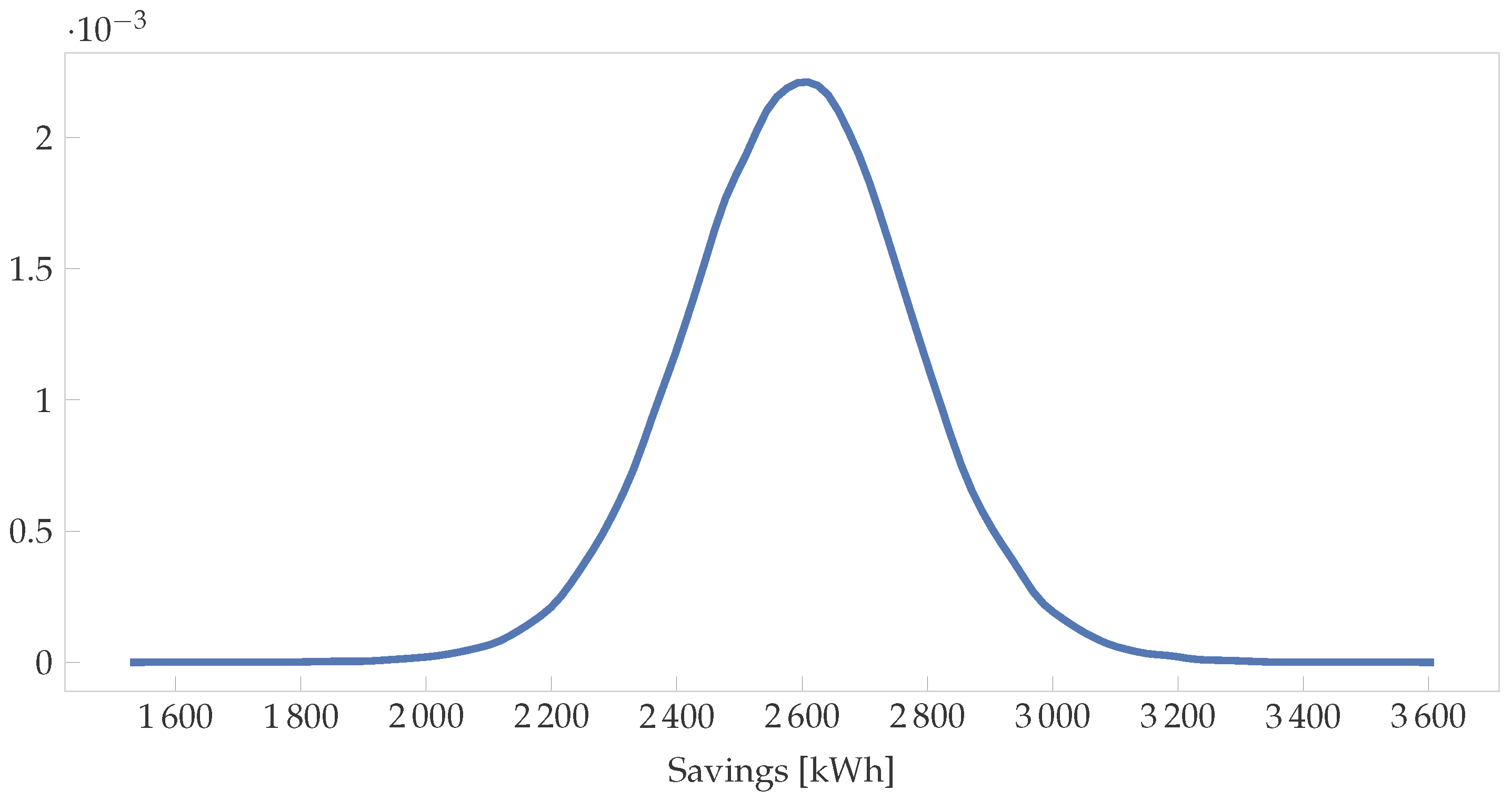
Figure 6.
Demonstration of robustness of t-distributed Bayesian regression. Note that the two Bayesian regression lines (solid and dashed) coincide almost perfectly.
Figure 6.
Demonstration of robustness of t-distributed Bayesian regression. Note that the two Bayesian regression lines (solid and dashed) coincide almost perfectly.

Table 1.
Cooling Degree Day (CDD) Data for International Performance Measurement and Verification Protocol (IPMVP) Example B-6. Note that these data were reverse-engineered to yield the same regression results as reported in the IPMVP. The original data were not reported in the IPMVP.
Table 1.
Cooling Degree Day (CDD) Data for International Performance Measurement and Verification Protocol (IPMVP) Example B-6. Note that these data were reverse-engineered to yield the same regression results as reported in the IPMVP. The original data were not reported in the IPMVP.
| Month | Jan | Feb | Mar | Apr | May | Jun | Jul | Aug | Sep | Oct | Nov | Dec |
|---|---|---|---|---|---|---|---|---|---|---|---|---|
| CDD | 312 | 292 | 222 | 112 | 92 | 22 | 12 | 32 | 157 | 207 | 182 | 302 |
| Energy Use | 7823 | 7585 | 7486 | 6646 | 6185 | 5933 | 5381 | 5917 | 7158 | 7064 | 7231 | 8250 |
Table 2.
Linear regression fit characteristics for data in Table 1. The coefficient of determination is , which is identical to the IPMVP case. These results may be compared to Bayesian summary statistics in Table 3.
| Parameter | Value | Standard Error | 95% Interval |
|---|---|---|---|
| Slope coefficient | 7.75 | 0.67 | [6.26, 9.23] |
| Intercept coefficient | 5634 | 129 | [5347, 5921] |
Table 3.
Summary statistics for Bayesian posterior distributions shown in Figure 3 when a Student’s t-distribution is used on the likelihood. Compare to linear regression results in Table 2. HDI: Highest Density Intervals.
| Parameter | Value | 95% HDI |
|---|---|---|
| Slope coefficient | 7.69 | [6.21, 9.24] |
| Intercept coefficient | 5634 | [5351, 5937] |
Table 4.
Common M&V (Measurement and Verification) cases and their Bayesian alternatives.
| Problem Type | Variant | Bayesian Alternative | Example Reference |
|---|---|---|---|
| Sampling | Single Sample | Section 3.1, [2] | |
| Randomised Control Trial | Bayesian Estimation | [42] | |
| ANOVA | Hierarchical modelling | [64] | |
| Regression | Standard | Bayesian regression | Section 3.2, [19] |
| With change points | Bayesian regression | [17] | |
| Pooled fixed effects | Hierarchical modelling | [63] | |
| Non-parametric | Gaussian Process | [39,65,66] | |
| Longitudinal | Persistence | Dynamic Generalised | [20] |
| Linear Model | |||
| Meter calibration | Simulation Extrapolation | [67] | |
| with Bayesian refinement |
© 2018 by the authors. Licensee MDPI, Basel, Switzerland. This article is an open access article distributed under the terms and conditions of the Creative Commons Attribution (CC BY) license (http://creativecommons.org/licenses/by/4.0/).
Share and Cite
MDPI and ACS Style
Carstens, H.; Xia, X.; Yadavalli, S. Bayesian Energy Measurement and Verification Analysis. Energies 2018, 11, 380. https://doi.org/10.3390/en11020380
AMA Style
Carstens H, Xia X, Yadavalli S. Bayesian Energy Measurement and Verification Analysis. Energies. 2018; 11(2):380. https://doi.org/10.3390/en11020380
Chicago/Turabian StyleCarstens, Herman, Xiaohua Xia, and Sarma Yadavalli. 2018. "Bayesian Energy Measurement and Verification Analysis" Energies 11, no. 2: 380. https://doi.org/10.3390/en11020380
Note that from the first issue of 2016, this journal uses article numbers instead of page numbers. See further details here.