Development of Easily Accessible Electricity Consumption Model Using Open Data and GA-SVR


1
Institute for Environmental Design and Engineering, Bartlett, University College London, 14 Upper Woburn Place, London WC1H 0NN, UK
2
Department of Economics, Hansung University, 116 Samseongyoro-16Gil, Seongbuk-Gu, Seoul 02876, Korea
3
Department of Architectural Engineering, Hanyang University, 222 Wangsimni-Ro, Seungdong-Gu, Seoul 133791, Korea
*
Author to whom correspondence should be addressed.
Energies 2018, 11(2), 373; https://doi.org/10.3390/en11020373
Submission received: 29 December 2017
/
Revised: 26 January 2018
/
Accepted: 30 January 2018
/
Published: 5 February 2018
(This article belongs to the Special Issue Building Energy Use: Modeling and Analysis)
Abstract
:In many countries, DR (Demand Response) has been developed for which customers are motivated to save electricity by themselves during peak time to prevent grand-scale blackouts. One of the common methods in DR, is CPP (Critical Peak Pricing). Predicting energy consumption is recognized as one of the tool for dealing with CPP. There are a variety of studies in developing the model of energy consumption, which is based on energy simulation, data-driven model or metamodelling. However, it is difficult for general users to use these models due to requirement of various sensing data and expertise. And it also takes long time to simulate the models. These limitations can be an obstacle for achieving CPP’s purpose that encourages general users to manage their energy usage by themselves. As an alternative, this research suggests to use open data and GA (Genetic Algorithm)–SVR (Support Vector Regression). The model is applied to a hospital in Korea and 34,636 data sets (1 year) are collected while 31,756 (11 months) sets are used for training and 2880 sets (1 month) are used for validation. As a result, the performance of proposed model is 14.17% in CV (RMSE), which satisfies the Korea Energy Agency’s and ASHRAE (American Society of Heating, Refrigerating and Air-Conditioning Engineers) error allowance range of ±30%, and ±20% respectively.
1. Introduction
Electric consumption is on the increase, which is turning out to be the woes of many countries. DR (Demand Response) has been introduced by which the customers in the electricity market are motivated to save electricity during peak time for preventing grand-scale blackouts from the unconscious use of electricity [1,2,3]. There are a host of different programs for DR, according to each country’s policy [4]. One of the common methods is CPP (Critical Peak Pricing), which is to calculate electric charges based on the highest value of average electricity consumption during certain time gap [5].
Predicting energy consumption is recognized as one of the tool for dealing with CPP. There are a variety of studies in developing the model of energy consumption [6,7,8,9,10,11,12,13,14], which is based on energy simulation or data-driven model, and metamodeling. However, it is difficult for general user to use these models due to requirement of various sensing data and expertise. And it takes a long time to generate energy consumption model. This limitation can be an obstacle for achieving CPP’s purpose that encourages general users to manage their energy usage by themselves.
Open data is big data managed by government and public institutions in various areas such as architecture, energy, traffic. According to countries, since policy of releasing open data is different, the empowerment of general users and type of open data vary [15,16]. For example, the Korean government provides open data such as temperature, humidity, insolation, wind speed, sea level atmospheric pressure, typhoon, electricity consumption, subway ride statistics, and energy efficiency rating. Among these, some of data are required to be charged and approved from the person in charge.
As energy data related to energy consumption such as temperature and humidity shows nonlinear patterns, making good a model requires the best prediction method that is capable of recognizing the data [17]. SVR (Support Vector Regression) is a machine learning algorithm that learns nonlinear data to predict a dependent variable, which is the occurrence of over-fitting problems is lower and it displays greater prediction performance [18,19,20]. However, three parameters (ε, , ) must be preset by users for improving SVR’s performance [17,21,22]. GA is one of the searching algorithm to explore the optimal solution [21,23].
In this paper, the aim is to model energy consumption employing GA-SVR and open data from Korean government, and make sure this model can be used or not. If the proposed approach can be employed, by following this, not only Korean but also other general users that can gain open data from their government can implement energy consumption model without the difficulties (expensive sensor, professional expertise, and long simulation time) for responding to CPP.
2. Literature Review on the Necessity of Proposed Approach and Design for Model Based on Machine Learning
2.1. The Necessity of Electricity Consumption Prediction Considering CPP
Generally, DR programs can be divided into two primary categories: IBP (Incentive Based Programs) and PBP (Price-Based Programs). IBP, which consist of various programs such as direct load control programs and interruptible load programs, is to pay incentive based on participation of consumers to save electricity consumption. PBP, which is also divided into TOU (Time of Use), CPP (Critical Peak Pricing), EDP (Extreme Day Pricing) and RTP (Real Time Pricing), is to estimate prices of electricity according to time and amount of energy usage. In the case of CPP, its estimation of fee can bring about excessive charge. For example, in Korea, if the highest fifteen minutes average electricity consumption marked during this year’s July amounts to 2000 kW and even if the record never again exceeds 2000 kW, the corresponding base charge is applied until the June of the following year. Therefore, consumers make strategies to avoid CPP by monitoring the value of prediction which is why, this program can bring about high electric bill.
2.2. Difficulties of User’s Access in Using Existing Energy Consumption Model
Predicting energy consumption is recognized as one of the tool for dealing with CPP. The prediction of electricity consumption demands a wide range of data related to the consumption such as temperature sensor, heat flux sensor, and PMV (Predicted Mean Value) sensor.
Yang et al. [6] uses weather compressor power was on or off, water temperature entering the extension machine and the ice machine, water temperature exiting the ice machine, outdoor humidity and temperature, existence and the amount of coolant in the ice tank and the cooler electricity consumption. Platon et al. [7] selects outdoor temperature and humidity, boiler outlet temperature, boiler vent and electricity consumption as the relevant data. This research has attempted to use various sensing data related to electricity consumption. However, as consumers must bear the cost of installing sensors, it can be financial burden.
Kolter et al. [8] takes advantage of tax assessor records and a GIS(Geographic Information System) database, which is come from website of governments, Cambridge, and utility bills. Dong et al. [9] uses weather data such as temperature, humidity and global solar radiation, and utility bills. For using these models, since consumers type their energy usage in person, it may be considered time-consuming.
Another energy modeling method is to use energy simulation tools such as EnergyPlus [24], ESP-r [25], TRNSYS [26], and DOE-2 [27], which is a technique based on physic principle and mathematical equations. However, as using these simulation programs are required to type various inputs such as building archetypes, occupancy types and HVAC (Heating, Ventilation, and Air-conditioning) information, this work is quite complex and needs to have expertise of energy [28]. To overcome these problems, many studies [10,11,12] try to simplify this modeling (e.g., researching representative of complex input). However, it is still difficult for general users to use this method.
Korolija et al. [13] uses building type, orientation, building fabrics, glazing ratio, glazing coating, overhang, day lighting internal source, and HVAC system for generating cooling and heating demand. And they apply regression analysis to the generated data for modeling energy consumption. Symonds et al. [14] uses built forms, wall types, location, epochs, and occupancy types. And SVR and ANN (Artificial Neural Network) are used as prediction methods. This methodology is called metamodeling, which is combined with energy simulation and machine learning. A disadvantage of these models is it takes long time to simulate energy consumption to be used as output of machine learning, due to usage of energy simulation, and it also needs to type professional information of building.
Therefore, since models mentioned above can be an obstacle for achieving CPP’s purpose that encourages general users to manage their energy usage by themselves, a solution is required to take into account easily accessible modeling.
2.3. Open Data Policy and Use Cases in Many Fields
Big data means various data created quickly such as figure data, image data, text data [29,30]. Although there has been big data for a long time in the world, due to a lack of technology for collecting, processing and analyzing data, it is difficult to utilize the big data. In these days, the development of high-performance hardware such as GPU (Graphic Processing Unit) and parallel processing technologies such as Hadoop [31], MapReduce [32] enable big data to be processed more quickly by sharing computation of data. Open data is kinds of big data managed by government and public institutions in various areas such as architecture, energy, traffic. Currently, many countries afford the open data to the public as open source with guidelines for utilizing the data [15,16].
According to countries, since policy of releasing open data is different, the empowerment of general users and type of open data vary [15]. In the case of Denmark, the Building and Dwelling Register opened their address data to general users free of charge in 2005. Before this policy, fee of data usage was charged for access, making the data inaccessible [16]. In January 2011, the government of Slovakia introduced a regime of unprecedented openness, requiring that all documents related to public procurement containing receipts and contracts be published online, and making the validity of public contracts contingent on their publication. Open data from OS (Ordnance Survey) helps any the UK company that takes advantage of a map for development of real estate, urban planning. For using some of this data, general users need to purchase that. Business Atlas is a platform, which is developed by the MODA (Mayor’s Office of Data Analytics) to share the market research information for shrinking the gap between small and large companies of New York. The tool helps small companies to access to gain high-quality data on the economic conditions in a given neighborhood to help decision-making to decide a new business space or expand their business [33].
There are a variety of models using open data in a wide range of fields such as healthcare, property and weather. For example, Application “OneDome” affords assessments of real estates and rent using noise data in airports, crime data and accessibility to traffic provided [34]. A Company “Egg Moon Studio” developed a program to predict weather and provide information of observable stars, according to user’s environment data such as humid, temperature and wind speed data [35]. “Climate Field View” is one of the applications made by a company “The Climate Corporation” to predict the damage of crops taking advantage of weather, soil and crops data [36].
2.4. Literature Review on Energy Consumption Prediction Methods
If accuracy of prediction model of electricity consumption is inaccurate using open data, the use of this model is useless, thus, an approach to improve prediction accuracy must be designed. Since related data such as temperature and humidity has nonlinear patterns, the prediction method must be applicable for nonlinearity. As ARIMA (Autoregressive Integrated Moving Average) model, Fourier series and regression analysis are appropriate for linear data, these means of analysis are inadequate to expect high prediction level in forecasting electricity consumption [17]. On the other hand, machine learning is a method to analyze nonlinear patterned data. SVR, ANN, CBR (Case Based Reasoning) and DT (Decision-making Tree) all fall into the category of machine learning. Compared to other machine learning, SVR has less appearance of overfitting. This has been verified through studies from diverse fields covering prediction of electricity consumption, tourism demand, bankruptcy, wind speed, protein structural classes, stock markets, and financial time series [19,20,23,37,38,39,40,41].
2.5. SVR
SVR is a machine learning proposed by Vapnik [42] on the basis of structural risk minimization, minimizing the upper bound of generalization error, unlike other conventional algorithms based on empirical risk minimization [43,44,45]. Machine learning can commonly serve as classification, regression, and clustering. There are variety of performance evaluation methods and in case of SVR’s generalization of regression, RMSE (Root Mean Square Error) can be mainly used for assessment of performance. As shown on (1), RMSE takes square of the difference between the reference model value and the predicted value of arbitrary case point sets and the greater the number of case sets are the higher the prediction model accuracy evaluation becomes. The result’s proximity to 0 corresponds to the performance of the SVR:
The value of RMSE also can be used for one of the indicators to know the appearance of overfitting and underfitting, which are major problem to make low accuracy. While overfitting is to train data is excessively trained for only training model, underfitting is not well trained due to a lack of data. To solve both problems, enough data with good quality is supplied to train model. Also, it is difficult to decide the number of data for splitting appropriately the entire data into training data and validation data. If training data is set too small, insufficient data availability for modeling yields a model with low performance than its potential output. Oppositely, immoderate train data selection diminishes the credibility of the performance evaluation because the data for validation is scarce. Thus, generally train data and validation are divided into 80~90% and 10~20% respectively. The separation method for learning and validation data also poses another problem. The model can become biased if, by chance, training and validation data are selected in a way where the validation data gives a high performance. In this case cross-validation corrects such shortcoming. Cross-validation repeats modeling and evaluating k -times, each time with different training and validation data division, where this is called k -fold Cross-Validation. Conventionally, k equals 5 [46]. SVR consists of two types; linear SVR and nonlinear SVR.
2.5.1. Linear SVR
When training data are paired with vector , and when the target value of , corresponding to a given input value is within the deviation of , a linear SVR regression can be defined as a problem finding in a range as narrow as possible (2). Accordingly, while it does not allow deviation to be greater than , linear SVR discards the solutions within the deviation. Therefore, the goal is to achieve the flattest hyper plane most apt to the given data:
While the value of b in Equation (2) represents biases, corresponds to the slope of . Thus, when is small, the slope lowers. To solve this equation, the Euclidean norm has to be minimized, in which this problem can be regarded as a convex optimization problem (3):
As a solution to the problem, two slack variables are applied to newly derived optimization equations, where one is for when target value is below (4).
Among the elements of SVR, sets the threshold on the prediction error between target value and predicted value ’ considering other influential data, it expands the permitted error range to enhance SVR’s regression and generalization performance, augmenting the prediction model’s accuracy. As ignores errors with a certain extent from the target value, when the slack variables , are applied, data that are in is omitted while the outer data errors are measured by the slack variables.
Also, due to the innate errors of the data, possible solution cannot be found. For a proper separation boundary layer to exist, an appropriate value of parameter C arranges the error data. While a large value of C levies greater penalty on errors which minimizes the errors to a level of low generalization, a diminutive value of C affects the errors with a small penalty leading to a high generalization level on the errors. Thus, selecting an adequate value of C can improve the performance of the generalization of SVR [47].
2.5.2. Nonlinear SVR
In a case where data follows a nonlinear pattern as in Figure 1, an additional dimension axis, with the introduction of kernel function, can separate the data from a single hyper-plane through an optimal separation plane. The kernel functions can be as simple as the square of the data or they can be a combination of other complex functions. Typical kernel functions are polynomial, radial and sigmoid types. However, RBF (Radial Basis Function) generally has superior effect on the generalization of SVR than others [48].
To use a kernel function, Lagrange function can be used in above objective function and constraint function of (4). Lagrange multipliers can be derived as shown in (5):
As a result, when (6) is solved, a regression function in the form of the following equation can be reached:
Here, can be described into diverse forms of functions and if RBF function is chosen, can be utilized. As shown, while SVR can analyze nonlinear pattern data through kernel function, it is capable of mitigating overfitting phenomenon occurring in generalization through the application of C and . Nonetheless, despite the data in consideration being continuous, if the parameters are altered, the algorithm’s performance will change also. In order to intensify its predicting ability, the parameters’ optimum combination must be found [17,21,22].
2.6. GA
Grid Search, One Search, Cross Validation, Genetic Algorithm and Simulated Annealing are some of the ways to find the most suitable parameter combination. Among these, Since GA generates multiple values at the same time, it can arrive at the solutions quicker than other technique, with relatively lower chance of premature convergence and trials and errors [21,23].
GA selects the superior genes of the early generation and passes them down to the next generation and through crossover and mutation, it models an evolving process where the genes that adapt to the environment survive. The mechanism in obtaining the ideal parameter combination is shown in Figure 2. First, (1) the information related to the value of interest such as the value’s precision, the number of parameters, domain, selection of superior value, fitness function is input and then (2) initial population of solution is created randomly. (3) Fitness of each solution is assessed and if it satisfies the terminal criteria, the process ends. However, (5) if not, the process proceeds to the selection operator. These compose the arbitrary initial population. Then, the selection operator selects superior parental values for crossover where better genes are chosen by probability according to their suitability. Although there are many options to the operator, including roulette wheel choice and tournament selection, their common goal must be that superior genes have higher chance of selection. After the selection operator, crossover operator (6) takes place to pass down the chosen genes to the next generation without destroying their characteristics. (7) Mutation is process for searching wider solutions by changing or conserving original solutions. That probability of mutation is adjusted to user’s input. Afterwards, selection, crossover and mutation are repeatedly processed until the population satisfies function assessment that the user set fitness.
2.7. Energy Consumption Model’s Evaluation Methods
Many studies define standards of good prediction model. Fels et al. [49] mentions that CV (RMSE) of 7% above is recognized as “good” models. Reddy [50] suggests that CV (RMSE) of 5% below is seen as excellent models, 10% below of that is good models, and 20% below of that is regarded as mediocre models and in case of 20% above, it is considered to be poor models. ASHRAE Guideline 14-2002 [51] points out that value of CV (RMSE) is permitted until 20% at most as good baseline models. In the government of Korea, the allowance standard on prediction model as good models is in 30% of CV (RMSE)’s value.
3. Model Development Based on GA-SVR and Open Data
3.1. Data Selection
Table 1 is the list of public data provided by the government and related organizations for free. KEPCO (Korea Electronic Power Corporation) (total electricity consumption data by 15 min cycle), the National Weather Service (temperature, humidity, insolation, wind speed, sea level atmospheric pressure, and presence of typhoon), the Ministry of Land, Infrastructure and Transport (plottage, floor area, and electricity efficiency rating per building) offer data to the public in multiple formats such as JSON, CSV and XLS without charge. As the open data policy of Korean government, all data above can be used for free on (https://www.data.go.kr/), after agreement of each manager. In addition to the sources in the Table 1, other diverse data are open to the public including water works analysis, microorganism, inorganic concentration data on water works purification plant, and budget by year. Also, each data provided from Korean government can be different depending on users and buildings. For example, while weather data collected during 20 years of the past can be collected in any place, in the case of electric consumption, buildings that introduce relatively a smart meter earlier have more that data. Beside, according to contract methods with government and users, ranges of data such as space and sector can be different. In some data, since Korea is a divided country, some of buildings cannot release open data.
Variables used in existing research related to the prediction of electricity consumption are GDP (Gross Domestic Product), population, outdoor temperature, humidity, electricity consumption, insolation, the condition of compressor, temperature of water entering and leaving into the ice machine, existence and the amount of coolant in the ice tank, boiler outlet temperature, boiler vent and wind speed [6,7,52,53,54,55]. Among these, outdoor temperature, humidity, wind speed and electricity consumption could be induced from the list of open data provided from Korea government. A site for applying this model is a hospital in Hanyang University, which is under an effect of CPP. Total floor area of this building is 39,888.8 m2 with eighteen stories above ground and three below. And, this building’s annual total energy consumption needs and are about 16,500 MWh and the number of staff is estimated at about 1780 staffs (doctors: 510, nurses: 550 other jobs: 720). The state of practice is 68,000 ambulatory cares and 234,000 hospitalizations on average every year.
3.2. Properties of Data and Its Processing
The data on outdoor temperature and outdoor humidity are offered by minutes distinguished by each local constituency. As of the electricity consumption data, they cover each building by fifteen minutes unit. Among these, wind speed and humidity data, given in JSON format, are processed into CSV format in fifteen minutes unit, corresponding to the format of the electricity consumption data. Above mentioned earlier, to for using GA-SVR, enough data including input and output is required to train this model due to overfitting and underfitting. Therefore, in total 35,040 (1 year) cases of data consisting of outdoor temperature, outdoor humidity, wind speed and electricity consumption, training and validation data are defined as 80~90% and 10~20% respectively. However, 404 cases with missing or outlier data due to sensor errors were neglected to have 34,636 (1 year) appropriate cases. Then, they were divided into 31,756 training data sets (case 1~case 31,756) (about 11 months) and 2880 validation data sets (case 31,757~case 34,636) (about 1 month) (Table 2).
3.3. Model Generation Using Open Data and GA-SVR
Since it is difficult for general users to understand the theory GA-SVR, “R”, which is one of the free coding programs, is used for employing libraries. “R” provides many libraries such as ANN, SVR and DT, which is perfectly coded from the worldwide experts. In this research, for using SVR, the library of “e1071” is used and in the case of GA, the library name is “GA”. To combine GA and SVR, the objective function in GA is to find , and of SVR to make the lowest value of RMSE.
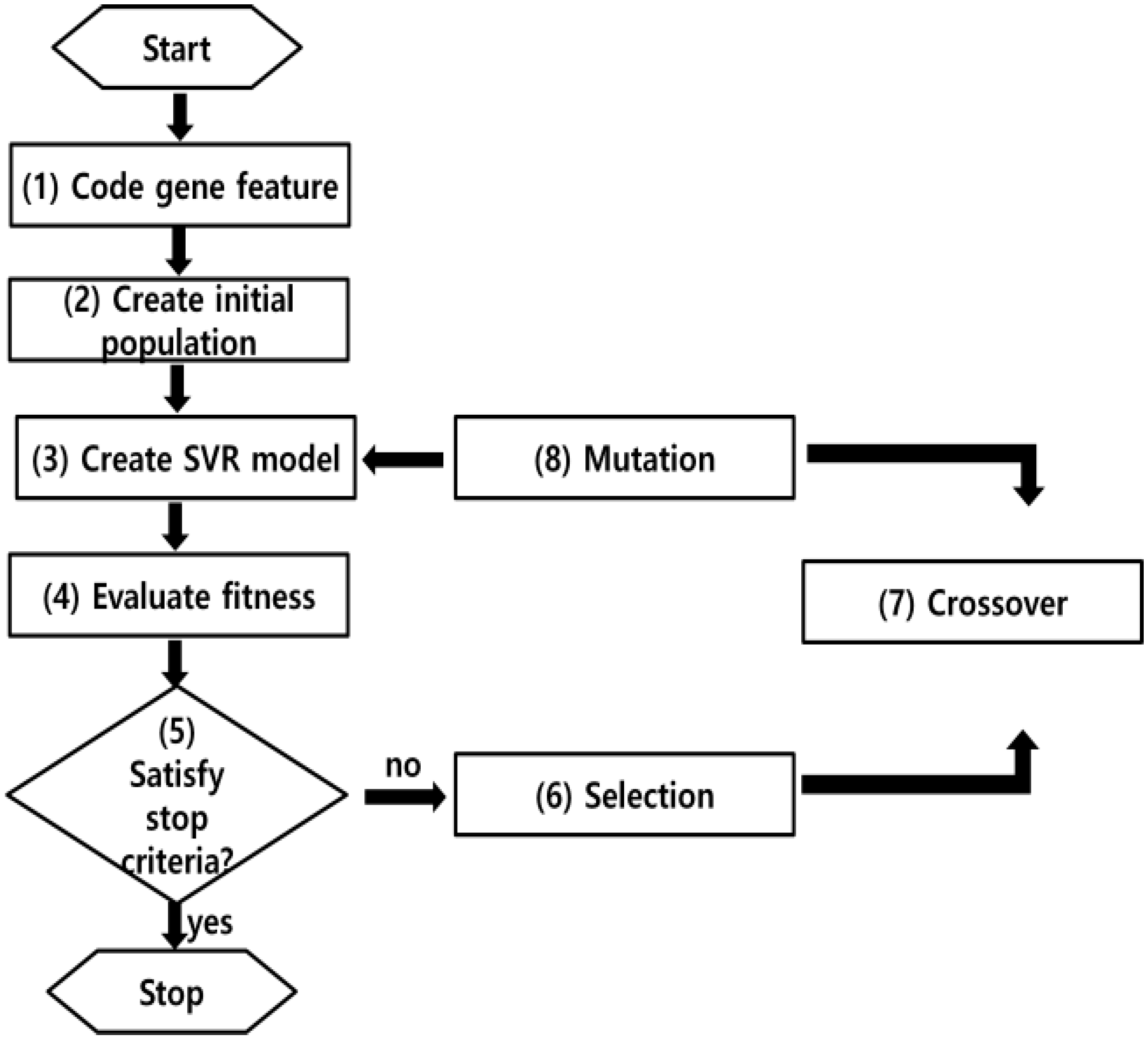
For training model, (1) SVR’s three parameters ’s initial values were each set as 1 × 10⁻³, 1 × 10⁻² and 1 × 10⁻⁴, while their maximum values were each bound to 1.7, 2 and 200 respectively. Also, initial value population of 500 values, 5000 generations, chance of superior value selection being 0.1, crossover probability of 0.8, 0.1 mutation rate configures the algorithm. The fitness function is cross validation based, where its RMSE value is the smallest. (2) On this basis, 500 arbitrary populations are formed and (3) each of these value population is utilized as trained SVR models’ parameters. (4) Subsequently, these models are evaluated by CV (RMSE) fitness function assessment and if satisfied, the process terminates. If not, (6) the selection operator is executed by roulette wheel method. Then, GA generates a new generation of values through (7) crossover operator and (8) mutation process so that the population equals 500, amounting to the number of the older generation. On 31,756 training data, the described procedure of selection, crossover and mutation is reiterated to the point where the parameters allowing the minimal CV(RMSE) value are acquired. This process is repeated until the SVR model can have the lowest value of CV (RMES) (Figure 3).
4. Applicability of Model Using Open Data and GA-SVR
The model is built on Intel® Core™ i7-7820HK [email protected] GHz, RAM 32.0 GB, and NVIDIA GeForce GTX 1080. Although GPU could be applied by employing this computer used to reduce computation time, it is not used. Since GA finds all parameters available for recognizing input (temperature, humidity and wind speed) and output (energy consumption) in training data, it takes 3 h in computation time at first. And the generated model could gain the predicted value immediately when inputs are typed in validation data. Unlike the approaches based simulation, this is one of the advantages in using machine learning approach [28].
GA could find three parameter values = 29.422, = 0.0997, and = 0.015 that make RMSE value of 82.01 when applied to the 2880 validation data (case31758~case34636).
The average of error rate (11.62%) shown on Table 3 is computed by dividing the absolute value of difference between the prediction values and the actual values by the actual value. The value of CV (RMSE) (14.17%) is calculated by dividing RMSE (82.01) by the average actual value (578.88 Kw) with converting it into percentage, which is well within the error allowance of ±30%.
Table 4 shows the difference in accuracy between the proposed model and other research’s models. In this comparison, it is assumed that the best prediction methods are applied in each model for their own dataset given that machine learning is black-box model. It means that it is difficult to decide the best prediction method with its parameters. In this research, unlike the research above, three parameters of SVR are selected using GA given that general users may have no deep knowledge about energy consumption and machine learning. Firstly, despite the fact that the proposed model, Platon et al. [7] and Bagnasco et al. [56] collect data during the same year, the latter two are better in accuracy. One of these reasons is due to a lack of open data quality. Some studies related to open data policy also point out this limitation in using open data [15,33]. In the case of Jain et al. [57] and Li et al. [58], although they take advantage of sensing data installed in their building in person, their accuracy is lower than the proposed model. This is because machine learning such as SVR, ANN, and DT requires users to collect enough train data to model. In the real world, it is difficult to collect enough train data. Edwards et al. [59] uses the greatest number of sensors, which is 140 sensors. However, the results refer to just 24.32% in ANN and 21.32% in SVR due to insufficient number of data to be trained for the model. Machine learning`s another name is data-driven model, which require a lot of train data. When compared to the proposed model and the model that reduces the number of train data of proposed model by half, its accuracy decrease to 43.26%. For using open data, general users do not need to collect and install sensor since governments already store a variety of data. In addition, although a lot of sensors are installed and its quality is good, if the number of sensing data is not enough to train model, it is difficult to generate appropriate energy consumption model. The reason is that the number of data has huge effects on performance of machine learning. There is no doubt that when compared to other models using sensing data, the proposed model’s accuracy is lower than those. However, for general users, it is easy to collect this open data and by using GA-SVR, professional expertise is not relatively required unlike using energy simulation. Moreover, the proposed model employing open data and GA-SVR can be used, since the value of CV (RMSE) satisfies the Korea Energy Agency’s and ASHRAE error allowance range of ±30%, and ±20% respectively.
5. Conclusions
Energy prediction model is recognized as an alternative for dealing with CPP. For using some model such as model based on energy simulation and metamodeling, general users need professional knowledge, and in the case of data-driven model, it is required to collect sensing data in person. An aim of this research is to suggest an easily accessible model for general users and make sure whether this model can be used or not. Open data of hospital provided from Korean government is just used as one of the case among many buildings to guide general users in the world for modelling energy consumption. In addition, this research introduces GA-SVR that takes account of nonlinear patterned data to improve its prediction accuracy with selecting the parameters. As a result, the proposed model’s accuracy is 14.17% in CV (RMSE), which satisfies the Korea Energy Agency’s error allowance range and ASHRAE error allowance range of ±30%, and ±20% respectively. Thus, they can use this proposed approach after making sure their country’s policy and data.
It is clear that the proposed model’s accuracy is lower than other models that collect enough sensing data to be trained. This is because open data quality is not better than sensing data installed in each building. However, it is difficult to secure enough good data to train model in the real world and it is time-consuming and expensive. There are some limitations and specifications for employing the proposed approach. First, since the number and quality of open data provided rely on each government’s policies and technologies, in some country, it can be difficult to predict other level’s consumption such as sector, and zone and to secure enough data. In addition, it is not guaranteed that GA-SVR can achieve the high performance of accuracy in other buildings. The reason is that machine learning approach is the heuristic approach in selecting parameters. Therefore, in the future research, review of best prediction method and their parameters in certain specification is needed for general users.
This research contribution is to consider viewpoint of general users and suggest new energy consumption model using open data and GA-SVR to encourage general users for dealing with CPP. According to each country’s open data policy, types, formats, frequency, and number of open data are different. Therefore, if some countries provide better quality data and enough data to be trained when compared to the case of Korea, the model using open data and GA-SVR is much better than a case in Korea.
Author Contributions
The contributions of each author are as follows: Seunghyeon Wang designed the research, analyzed the data, coded the programs, and compared existing research in the data used, accuracy and duration. Hyeonyong Hae checked the program and considered whether library could be used for prediction. Juhyung Kim helped to collect the open data, clarified the logic of background, and managed the overall research.
Conflicts of Interest
The authors declare no conflict of interest.
References
- Herter, K. Residential Implementation of Critical-Peak Pricing of Electricity; Lawrence Berkeley National Laboratory: Berkeley, CA, USA, 2006.
- Kii, M.; Sakamoto, K.; Hangai, Y.; Doi, K. The effects of critical peak pricing for electricity demand management on home-based trip generation. IATSS Res. 2014, 37, 89–97. [Google Scholar] [CrossRef]
- Hu, Z.; Kim, J.-H.; Wang, J.; Byrne, J. Review of dynamic pricing programs in the U.S. and Europe: Status quo and policy recommendations. Renew. Sustain. Energy Rev. 2015, 42, 743–751. [Google Scholar] [CrossRef]
- Zhang, Q.; Li, J. Demand response in electricity markets: A review. In Proceedings of the 2012 9th International Conference on the European Energy Market, Florence, Italy, 10–12 May 2012; pp. 1–8. [Google Scholar]
- Albadi, M.H.; Albadi, M.H.; El Saadany, E.F. A summary of demand response in electricity markets. Electr. Power Syst. Res. 2008, 78, 1989–1996. [Google Scholar] [CrossRef]
- Yang, J.; Rivard, H.; Zmeureanu, R. On-line building energy prediction using adaptive artificial neural networks. Energy Build. 2005, 37, 1250–1259. [Google Scholar] [CrossRef]
- Platon, R.; Dehkordi, V.; Martel, J. Hourly prediction of a building’s electricity consumption using case-based reasoning, artificial neural networks and principal component analysis. Energy Build. 2015, 92, 10–18. [Google Scholar] [CrossRef]
- Kolter, J.Z.; Ferreira, J., Jr. A Large-Scale Study on Predicting and Contextualizing Building Energy Usage. In Proceedings of the Twenty-Fifth AAAI Conference on Artificial Intelligence, San Francisco, CA, USA, 7–11 August 2011. [Google Scholar]
- Dong, B.; Lee, S.E.; Sapar, M.H. A holistic utility bill analysis method for baselining whole commercial building energy consumption in Singapore. Energy Build. 2005, 37, 167–174. [Google Scholar] [CrossRef]
- Liu, G.; Liu, M. A rapid calibration procedure and case study for simplified simulation models of commonly used HVAC systems. Build. Environ. 2011, 46, 409–420. [Google Scholar] [CrossRef]
- Liu, M.; Song, L.; Wei, G.; Claridge, D. Simplified building and air handling unit model calibration and applications. In Proceedings of the ASME 2003 International Solar Energy Conference, Kohala Coast, HI, USA, 15–18 March 2003; pp. 15–25. [Google Scholar]
- Turiel, I.; Boschen, R.; Seedall, M.; Levine, M. Simplified energy analysis methodology for commercial buildings. Energy Build. 1984, 6, 67–83. [Google Scholar] [CrossRef]
- Korolija, I.; Zhang, Y.; Marjanovic Halburd, L.; Hanby, V. Regression models for predicting UK office building energy consumption from heating and cooling demands. Energy Build. 2013, 59, 214–227. [Google Scholar] [CrossRef]
- Symonds, P.; Taylor, J.; Chalabi, Z.; Mavrogianni, A.; Davies, M.; Hamilton, I.; Vardoulakis, S.; Heaviside, C.; Macintyre, H. Development of an England-wide indoor overheating and air pollution model using artificial neural networks. J. Build. Perform. Simul. 2016, 9, 606–619. [Google Scholar] [CrossRef]
- Huijboom, N.; Van den Broek, T. Open data: An international comparison of strategies. Eur. J. ePract. 2011, 12, 4–16. [Google Scholar]
- Kassen, M. A promising phenomenon of open data: A case study of the Chicago open data project. Gov. Inf. Q. 2013, 30, 508–513. [Google Scholar] [CrossRef]
- Jung, H.C.; Kim, J.S.; Heo, H. Prediction of building energy consumption using an improved real coded genetic algorithm based least squares support vector machine approach. Energy Build. 2015, 90, 76–84. [Google Scholar] [CrossRef]
- Avci, E. Selecting of the optimal feature subset and kernel parameters in digital modulation classification by using hybrid genetic algorithm–support vector machines: HGASVM. Expert Syst. Appl. 2009, 36, 1391–1402. [Google Scholar] [CrossRef]
- Wu, Q. The hybrid forecasting model based on chaotic mapping, genetic algorithm and support vector machine. Expert Syst. Appl. 2010, 37, 1776–1783. [Google Scholar] [CrossRef]
- Xuemei, L.; Lixing, D.; Yan, L.; Gang, X.; Jibin, L. Hybrid genetic algorithm and support vector regression in cooling load prediction. In Proceedings of the Third International Conference on Knowledge Discovery and Data Mining, WKDD’10, Phuket, Thailand, 9–10 January 2010; pp. 527–531. [Google Scholar]
- Huang, C.-L.; Wang, C.-J. A GA-based feature selection and parameters optimizationfor support vector machines. Expert Syst. Appl. 2006, 31, 231–240. [Google Scholar] [CrossRef]
- Son, H.; Kim, C.; Kim, C. Hybrid principal component analysis and support vector machine model for predicting the cost performance of commercial building projects using pre-project planning variables. Autom. Constr. 2012, 27, 60–66. [Google Scholar] [CrossRef]
- Chen, K.-Y.; Wang, C.-H. Support vector regression with genetic algorithms in forecasting tourism demand. Tour. Manag. 2007, 28, 215–226. [Google Scholar] [CrossRef]
- Crawley, D.B.; Lawrie, L.K.; Winkelmann, F.C.; Buhl, W.F.; Huang, Y.J.; Pedersen, C.O.; Strand, R.K.; Liesen, R.J.; Fisher, D.E.; Witte, M.J. EnergyPlus: Creating a new-generation building energy simulation program. Energy Build. 2001, 33, 319–331. [Google Scholar] [CrossRef]
- Free Software Foundation Inc. ESP-r, version 2; Free Software Foundation Inc.: Boston, MA, USA, 1996.
- University of Wisconsin. TRNSYS, version 14.2; University of Wisconsin: Madison, WI, USA, 1996.
- Winkelmann, F.; Birdsall, B.; Buhl, W.; Ellington, K.; Erdem, A.; Hirsch, J.; Gates, S. DOE-2 Supplement: Version 2.1; Lawrence Berkeley Lab: Berkeley, CA, USA, 1993. [Google Scholar]
- Foucquier, A.; Robert, S.; Suard, F.; Stéphan, L.; Jay, A. State of the art in building modelling and energy performances prediction: A review. Renew. Sustain. Energy Rev. 2013, 23, 272–288. [Google Scholar] [CrossRef]
- Kitchin, R. Big data and human geography: Opportunities, challenges and risks. Dialogues Hum. Geogr. 2013, 3, 262–267. [Google Scholar] [CrossRef]
- Chen, H.; Chiang, R.H.; Storey, V.C. Business intelligence and analytics: From big data to big impact. MIS Q. 2012, 36, 1165–1188. [Google Scholar]
- Borthakur, D. The hadoop distributed file system: Architecture and design. Apache Softw. Found. 2007, 11, 21. [Google Scholar]
- Dean, J.; Ghemawat, S. MapReduce: Simplified data processing on large clusters. Commun. ACM 2008, 51, 107–113. [Google Scholar] [CrossRef]
- Zuiderwijk, A.; Janssen, M. Open data policies, their implementation and impact: A framework for comparison. Gov. Inf. Q. 2014, 31, 17–29. [Google Scholar] [CrossRef]
- OneDome. Available online: http://www.onedome.com (accessed on 13 February 2017).
- Eggmoonstudio. Available online: http://eggmoonstudio.com/ (accessed on 13 February 2017).
- Climate Field View. Available online: https://www.climate.com/ (accessed on 13 February 2017).
- Min, J.H.; Lee, Y.-C. Bankruptcy prediction using support vector machine with optimal choice of kernel function parameters. Expert Syst. Appl. 2005, 28, 603–614. [Google Scholar] [CrossRef]
- Mohandes, M.A.; Halawani, T.O.; Rehman, S.; Hussain, A.A. Support vector machines for wind speed prediction. Renew. Energy 2004, 29, 939–947. [Google Scholar] [CrossRef]
- Sun, X.-D.; Huang, R.-B. Prediction of protein structural classes using support vector machines. Amino Acids 2006, 30, 469–475. [Google Scholar] [CrossRef] [PubMed]
- Tay, F.E.; Cao, L. Application of support vector machines in financial time series forecasting. Omega 2001, 29, 309–317. [Google Scholar] [CrossRef]
- Huang, W.; Nakamori, Y.; Wang, S.-Y. Forecasting stock market movement direction with support vector machine. Comput. Oper. Res. 2005, 32, 2513–2522. [Google Scholar] [CrossRef]
- Vapnik, V.N.; Vapnik, V. Statistical Learning Theory; Wiley: New York, NY, USA, 1998; Volume 1. [Google Scholar]
- Burges, C.J. A tutorial on support vector machines for pattern recognition. Data Min. Knowl. Discov. 1998, 2, 121–167. [Google Scholar] [CrossRef]
- Gunn, S.R. Support vector machines for classification and regression. ISIS Tech. Rep. 1998, 14, 85–86. [Google Scholar]
- Cristianini, N.; Shawe-Taylor, J. An Introduction to Support Vector Machines and Other Kernel-Based Learning Methods; Cambridge University Press: Cambridge, UK, 2000. [Google Scholar]
- Segaran, T. Programming Collective Intelligence: Building Smart Web 2.0 Applications; O’Reilly Media, Inc.: Sebastopol, CA, USA, 2007. [Google Scholar]
- Smola, A.J.; Schölkopf, B. A tutorial on support vector regression. Stat. Comput. 2004, 14, 199–222. [Google Scholar] [CrossRef]
- Keerthi, S.S.; Lin, C.-J. Asymptotic behaviors of support vector machines with Gaussian kernel. Neural Comput. 2003, 15, 1667–1689. [Google Scholar] [CrossRef] [PubMed]
- Fels, M.F.; Keating, K.M. Savings from demand-side management programs in us electric utilities. Annu. Rev. Energy Environ. 1993, 18, 57–88. [Google Scholar] [CrossRef]
- Reddy, T.A.; Saman, N.F.; Claridge, D.E.; Haberl, J.S.; Turner, W.D.; Chalifoux, A.T. Baselining methodology for facility-level monthly energy use-part 1: Theoretical aspects. In ASHRAE Transactions; ASHRAE: New York, NY, USA, 1997. [Google Scholar]
- Haberl, J.S.; Claridge, D.; Culp, C. ASHRAE’s guideline 14-2002 for measurement of energy and demand savings: How to determine what was really saved by the retrofit. In Proceedings of the Fifth International Conference for Enhanced Building Operations, Pittsburgh, PA, USA, 11–13 October 2005. [Google Scholar]
- Hsu, C.-C.; Chen, C.-Y. Regional load forecasting in Taiwan––Applications of artificial neural networks. Energy Convers. Manag. 2003, 44, 1941–1949. [Google Scholar] [CrossRef]
- Dong, B.; Cao, C.; Lee, S.E. Applying support vector machines to predict building energy consumption in tropical region. Energy Build. 2005, 37, 545–553. [Google Scholar] [CrossRef]
- Hong, W.-C. Electric load forecasting by support vector model. Appl. Math. Model. 2009, 33, 2444–2454. [Google Scholar] [CrossRef]
- Hayati, M.; Shirvany, Y. Artificial neural network approach for short term load forecasting for Illam region. World Acad. Sci. Eng. Technol. 2007, 28, 280–284. [Google Scholar]
- Bagnasco, A.; Fresi, F.; Saviozzi, M.; Silvestro, F.; Vinci, A. Electrical consumption forecasting in hospital facilities: An application case. Energy Build. 2015, 103, 261–270. [Google Scholar] [CrossRef]
- Jain, R.K.; Smith, K.M.; Culligan, P.J.; Taylor, J.E. Forecasting energy consumption of multi-family residential buildings using support vector regression: Investigating the impact of temporal and spatial monitoring granularity on performance accuracy. Appl. Energy 2014, 123, 168–178. [Google Scholar] [CrossRef]
- Li, N.; Kwak, J.-Y.; Becerik-Gerber, B.; Tambe, M. Predicting HVAC energy consumption in commercial buildings using multiagent systems. In Proceedings of the 30th International Symposium on Automation and Robotics in Construction and Mining, ISARC, Montréal, QC, Canada, 11–15 August 2013. [Google Scholar]
- Edwards, R.E.; New, J.; Parker, L.E. Predicting future hourly residential electrical consumption: A machine learning case study. Energy Build. 2012, 49, 591–603. [Google Scholar] [CrossRef]
Figure 1.
Application of kernel function to find nonlinear data’s optimal separation plane.
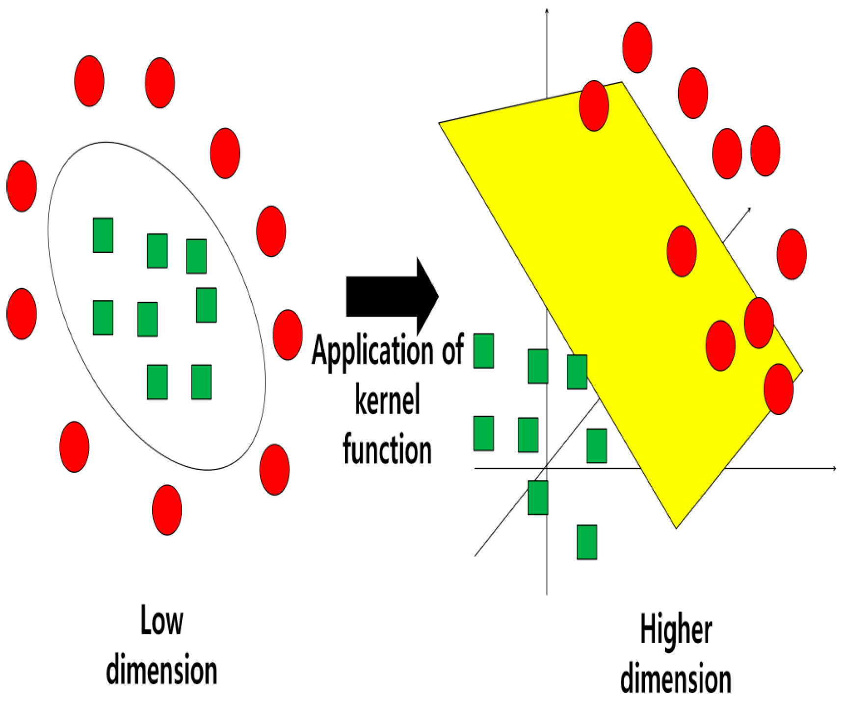
Figure 2.
Process for deducing optimal solution using Genetic Algorithm (GA).
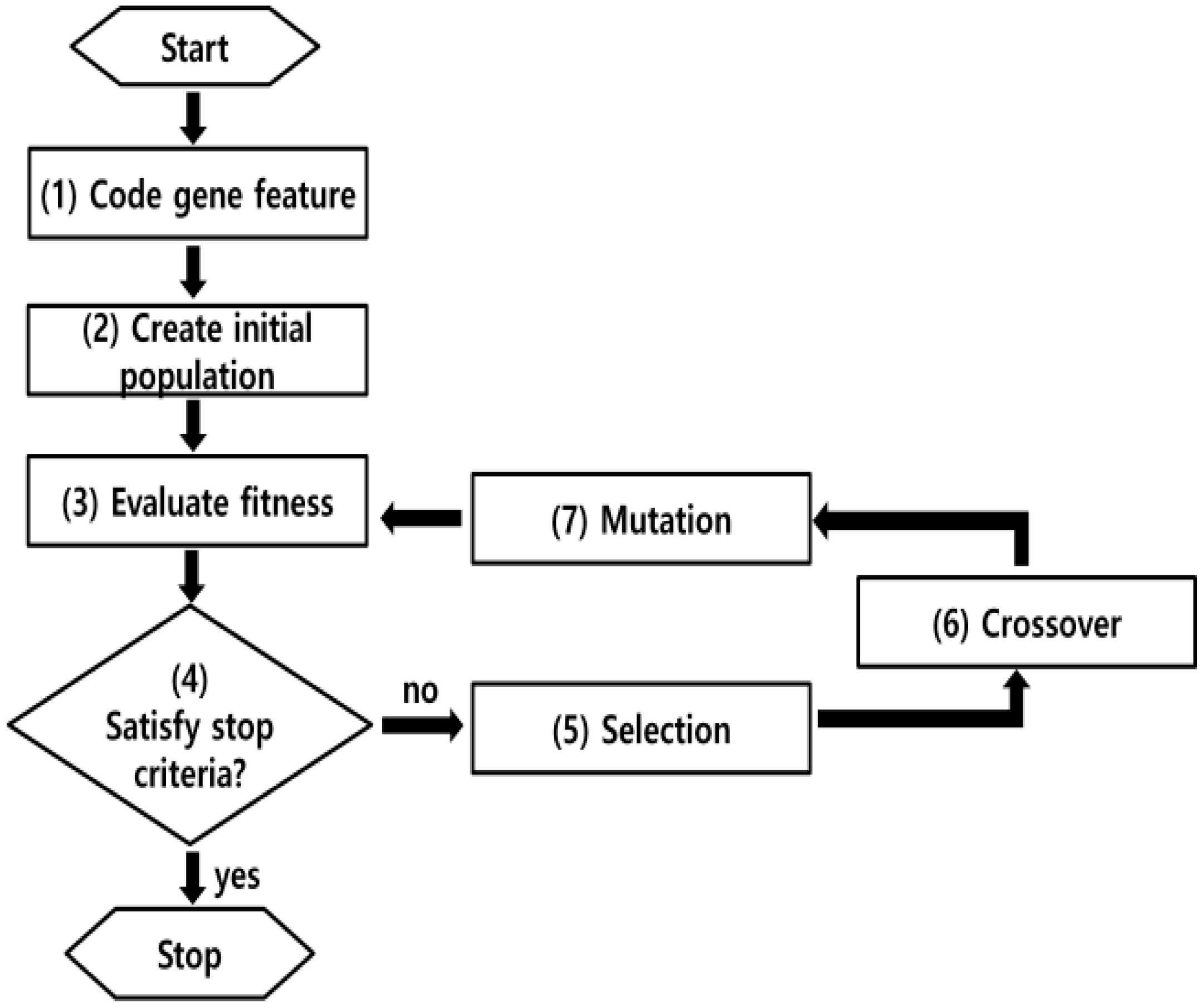
Figure 3.
Process to deduce three parameters (, ε, in Support Vector Machine (SVR).


Table 1.
Example of open data provided from Korean government.
| Data Type | Cycle | Format | Source |
|---|---|---|---|
| temperature, humidity, insolation, wind speed, sea level atmospheric pressure, presence of typhoon | 1 min | JSON | The National Weather Service |
| total electricity consumption | 15 min, daily | CSV | KEPCO |
| plottage, floor area, energy efficiency rating | Categorical data | JSON, CSV | Ministry of Land, Infrastructure and Transport |
| Seoul floating population | Categorical data | ETC, XLSX | Seoul City |
| subway ride statistics | Daily | CSV, XLS, XLSX | Seoul Metro |
Table 2.
Training data and validation data for Genetic Algorithm-Support Vector Machine (GA-SVR).
| Case | Temperature (°C) | Velocity (m/s) | Humidity (%) | Electricity Consumption (Kw) |
|---|---|---|---|---|
| case 1 | 25.3 | 1.2 | 89.8 | 454.56 |
| case 2 | 25.3 | 0.4 | 89.7 | 440.88 |
| case 3 | 25.2 | 1.7 | 89.7 | 438 |
| case 4 | 25.1 | 0.7 | 90.0 | 447.84 |
| case 5 | 25.1 | 1.2 | 91.0 | 459.36 |
| ~ | ||||
| case 34,632 | 27.3 | 1.4 | 77.5 | 493.44 |
| case 34,633 | 27.3 | 1.0 | 78.7 | 490.56 |
| case 34,634 | 27.1 | 1.7 | 79.3 | 486 |
| case 34,635 | 27.1 | 2.1 | 76.1 | 491.52 |
| case 34,636 | 26.9 | 3.1 | 76.0 | 480.24 |
Table 3.
Difference between the actual value and predicted value.
| Case | Actual Value (Kw) | Prediction (Kw) | Error Rate (%) |
|---|---|---|---|
| case 31,757 | 464.64 | 497.58 | 7.08 |
| case 31,758 | 459.6 | 494.10 | 7.50 |
| case 31,759 | 453.36 | 490.02 | 8.09 |
| case 31,760 | 435.12 | 484.45 | 11.33 |
| case 31,761 | 417.36 | 478.41 | 14.62 |
| ~ | |||
| case 34,632 | 493.44 | 508.77 | 3.10 |
| case 34,633 | 490.56 | 486.61 | 0.80 |
| case 34,634 | 486 | 493.42 | 1.52 |
| case 34,635 | 491.52 | 490.06 | 0.29 |
| case 34,636 | 480.24 | 488.85 | 1.79 |
| Average | 578.88 | 575.19 | 11.62 |
| RMSE | 82.01 | ||
| CV(RMSE) | 14.17% | ||
Table 4.
Comparison between the proposed model and other models.
| Reference | Prediction Method | Feature | Data Size | CV (RMSE) |
|---|---|---|---|---|
| the proposed model | GA-SVR | temperature, humidity wind speed | 1 year | 14.17% |
| the proposed Model | GA-SVR | temperature, humidity wind speed | 6 months | 43.26% |
| Platon et al. [7] | ANN | outside air temperature, outside air relative temperature, boiler outlet water temperature, boiler outlet water flow rate, chiller outlet water temperature, chiller outlet water flow rate, supply air temperatures—hot duct for AHUs (Air Handling Units), supply air temperatures-cold duct for AHUs, supply air D control settings for ahus, return air fan VFD (Variable Frequency Drive) control settings for AHUs, indoor air temperatures of different zones | 1 year | 7.30% |
| Bagnasco et al. [56] | ANN | date, 24-h-ahead average load, day-ahead load, 7 days-ahead load, day-ahead temperature | 1 year | 6.97% |
| Jain et al. [57] | SVR | temperature, date, sine of current hour, cosine of current hour | 3.5 months | 10.47~133.24% |
| Li et al. [58] | SVR | temperature, HVAC’s set point, | 8 months | 16.2% |
| Edwards et al. [59] | ANNSVR | 140 different sensors | 1 year | 24.32%21.32% |
© 2018 by the authors. Licensee MDPI, Basel, Switzerland. This article is an open access article distributed under the terms and conditions of the Creative Commons Attribution (CC BY) license (http://creativecommons.org/licenses/by/4.0/).
Share and Cite
MDPI and ACS Style
Wang, S.; Hae, H.; Kim, J. Development of Easily Accessible Electricity Consumption Model Using Open Data and GA-SVR. Energies 2018, 11, 373. https://doi.org/10.3390/en11020373
AMA Style
Wang S, Hae H, Kim J. Development of Easily Accessible Electricity Consumption Model Using Open Data and GA-SVR. Energies. 2018; 11(2):373. https://doi.org/10.3390/en11020373
Chicago/Turabian StyleWang, Seunghyeon, Hyeonyong Hae, and Juhyung Kim. 2018. "Development of Easily Accessible Electricity Consumption Model Using Open Data and GA-SVR" Energies 11, no. 2: 373. https://doi.org/10.3390/en11020373
Note that from the first issue of 2016, this journal uses article numbers instead of page numbers. See further details here.